Electromagnetic characteristics of ENSO

The motion of electrically conducting sea water through Earth's magnetic field induces secondary electromagnetic fields. Due to its periodicity, the oceanic tidally induced magnetic field is easily distinguishable in magnetic field measurements and therefore detectable. These tidally induced signatures in the electromagnetic fields are also sensitive to changes in oceanic temperature and salinity distributions. We investigate the impact of oceanic heat and salinity changes related to the El Niño–Southern Oscillation (ENSO) on oceanic tidally induced magnetic fields. Synthetic hydrographic data containing characteristic ENSO dynamics have been derived from a coupled ocean–atmosphere simulation covering a period of 50 years. The corresponding tidally induced magnetic signals have been calculated with the 3-D induction solver x3dg. By means of the Oceanic Niño Index (ONI), based on sea surface temperature anomalies, and a corresponding Magnetic Niño Index (MaNI), based on anomalies in the oceanic tidally induced magnetic field at sea level, we demonstrate that evidence of developing ENSO events can be found in the oceanic magnetic fields statistically 4 months earlier than in sea surface temperatures. The analysis of the spatio-temporal progression of the oceanic magnetic field anomalies offers a deeper understanding on the underlying oceanic processes and is used to test and validate the initial findings.

1 Introduction

The El Niño–Southern Oscillation (ENSO) is well known for its warm and cold temperature anomalies caused by changes in the ocean–atmosphere system in the equatorial Pacific Ocean. These anomalous events, known as El Niño and La Niña, cause extreme weather conditions throughout the globe, e.g. tropical cyclones (Vincent et al., 2011), droughts, bush fires and floods (Philander, 1983). The extreme weather affects entire ecosystems (Glynn and De Weerdt, 1991) and causes damage to infrastructure and agricultural production (Wilhite et al., 1987), with substantial socio-economic costs. The prospective doubling of extreme El Niño events, as a response to greenhouse warming (Cai et al., 2014), would increase the socio-economic costs even further. The negative impacts can be mitigated with preemptive measures provided reliable El Niño forecasts are available.

Knowledge about spatio-temporal variations of upper-ocean heat content, acquired traditionally by moorings, are a major source of ENSO predictability (Meinen and McPhaden, 2000). Monitoring of seawater temperature and salinity anomalies are consequently a prerequisite for improved ENSO forecasting, especially since changes in thermocline depth, caused by equatorial Kelvin waves, have been known to precede sea surface temperature anomalies (Harrison and Schopf, 1984). These anomalies are already measurable with an array of moored buoys (TAO/TRITON) which monitors the upper ocean temperature. Furthermore, measurement of the mentioned thermocline displacements with altimetric methods has been subject of extensive research (Ji et al., 2000; Picaut et al., 1996, 2002).

Changes in the oceanic heat content can also be inferred from the motion-induced electromagnetic fields of the ocean (Minami, 2017; Saynisch et al., 2016). This new and lesser-known method complements the pre-existing techniques. It can be applied to detect mainly large-scale oceanic processes altering temperature and salinity distributions.

The flow of electrically conducting seawater generates an electric current due to the interaction of moving salt ions with the geomagnetic field. These electric currents induce a magnetic field with a local magnitude of several nanotesla (nT; Maus and Kuvshinov, 2004).

Depending on the field strength of the ambient geomagnetic field, the magnitudes of ocean flow and electric seawater conductivity determine the ocean tide induced magnetic field strength. The ocean flow is classically divided into general ocean circulation and ocean tides.

The ocean circulation driven by momentum and buoyancy fluxes is irregular in time. Its effect are consequently difficult to separate from magnetic field measurements. However, the circulation-induced magnetic field's non-trivial contributions to the geomagnetic field have been subject of many studies (Irrgang et al., 2016a, b; Manoj et al., 2006; Tyler and Mysak, 1995). Manoj et al. (2006) analysed the influence of changes in the equatorial current system caused by ENSO on the circulation-induced magnetic field. They neglected temporal variations in oceanic temperature and salinity and assumed a time-constant oceanic conductivity distribution. In their study, the difference between the global circulation-induced magnetic field during normal conditions and El Niño conditions was estimated. They found that ENSO-related magnetic field anomalies in the equatorial region were too small to be distinguishable from the magnetic field anomalies caused by variations of the Antarctic circumpolar current (ACC). The large ACC anomalies extend into the equatorial region and over-shadow the small effect of ENSO. The magnitude of the ACC anomalies was found to be of ±0.2 nT at Swarm altitude (430 km) in the equatorial Pacific and can therefore be assumed to be an upper limit to ENSO's circulation-induced magnetic field anomalies.

The periodicity of the tidal flow, however, allows for an easy separation of its magnetic field from other constituents in geomagnetic field measurements. Its signals have been extracted successfully for the semidiurnal M2 and N2 tides from measurements of the magnetic satellite missions CHAMP and Swarm (Sabaka et al., 2016; Tyler et al., 2003). Amplitude variations of these periodic magnetic signals are mainly caused by variations in seawater conductivity distribution (Saynisch et al., 2016). Seawater conductivity is sensitive to seawater temperature and salinity. In comparison to the amphidromic system of the tides, these quantities exhibit high temporal variability. Consequently, the majority of information gained from anomalies of the oceanic tidally induced magnetic signals are linked to changes in oceanic temperature and salinity distributions. Modelled and measured tidally induced magnetic fields are in good agreement (Maus and Kuvshinov, 2004; Sabaka et al., 2016; Tyler et al., 2003), offering the possibility for in silico sensitivity studies.

The influences of global climate variations, such as Greenland glacial melting and global warming, on the electromagnetic oceanic tidally induced signals have already been investigated (Saynisch et al., 2016, 2017). For these cases, the tidally induced radial magnetic field was found to be an appropriate measure to monitor climate variations of the global oceanic conductivity on decadal timescales.

With a period of 4–7 years, ENSO acts on monthly to annual timescales. And despite its impact on the global climate, the immediate climatological influences on the ocean are limited to the region of the equatorial Pacific. ENSO's characteristic changes in the ocean circulation alter the Pacific upper ocean temperature and salinity distributions (≈ 300 m) within months.

In our study, we follow the approach of Saynisch et al. (2017) and investigate whether the electromagnetic oceanic tidally induced signals could be used as an appropriate measure for ENSO-induced changes in seawater conductivity and, consequently, the different stages in the dynamics of ENSO.

In Sect. 2, we introduce the oceanic electromagnetic induction along with the models and data used to compute the resulting climate sensitive electromagnetic oceanic tidally induced signals (EMOTSs). Also, based on the radial magnetic component of the modelled EMOTSs, we define a Magnetic Niño Index (MaNI). In Sect. 3, we compare the classic Oceanic Niño Index (ONI) to the proposed MaNI and discuss differences and similarities. We conclude and summarize the study in Sect. 4.

2 Models and data

2.1 Ocean data

We simulated ENSO with the ECHAM6/MPIOM, a global coupled atmosphere–ocean general circulation model (AOGCM; Giorgetta et al., 2013).

The Max Planck Institute Ocean Model (MPIOM, Jungclaus et al., 2013) is a general ocean circulation model. The model solves the primitive equations for a hydrostatic Boussinesq fluid on a curvilinear Arakawa C-grid with poles shifted to Antarctica and Greenland. The ocean is discretized on a grid with a horizontal resolution of ∼ 3.0^∘ × 1.8^∘ (GR30) and an irregular vertical distribution over 40 horizontal levels.

The atmosphere general circulation model ECHAM6 (Stevens et al., 2013) is applied with the horizontal resolution of ∼ 3.75^∘ × 3.75^∘ (T31) and 31 vertical hybrid sigma–pressure levels.

The simulated ocean data covers 50 years of monthly mean seawater temperature T, seawater salinity S and seawater pressure P. Using the Gibbs seawater equation (TEOS-10, IOC et al., 2010), the electric seawater conductivity σ can be calculated from, T, S and P. Present-day conditions were used to run the coupled AOGCM in a free mode instead of a observation-driven forcing. Therefore, the modelled climate represents reality only in a statistical sense.

2.2 Oceanic tidally induced currents and EMOTSs

The tidally induced electric current, the source for the electromagnetic oceanic tidal signals (EMOTSs), is derived for each month with the following two-step algorithm.

First, the product of seawater conductivity σ and tidal velocities v_M2 is integrated from ocean bottom (−H) to surface (SSH):

$$\begin{array}{}\text{(1)}& {\displaystyle }{\mathit{V}}_{\mathrm{M}\mathrm{2}}\left(\mathit{\phi },\mathit{\vartheta },t\right)=\underset{-\mathrm{H}}{\overset{\mathrm{SSH}}{\int }}\mathit{\sigma }\left(\mathit{\phi },\mathit{\vartheta },z,t\right)\cdot {\mathit{v}}_{\mathrm{M}\mathrm{2}}\left(\mathit{\phi },\mathit{\vartheta },z,t\right)\mathrm{d}z,\end{array}$$

where φ, ϑ and z are longitude, co-latitude and depth. The tidally induced electric current j_M2 is then calculated as the cross-product of the depth-integrated and conductivity-weighted transport V_M2 and the ambient geomagnetic field B_Earth as

$$\begin{array}{}\text{(2)}& {\mathit{j}}_{\mathrm{M}\mathrm{2}}\left(\mathit{\phi },\mathit{\vartheta }\right)={\mathit{V}}_{\mathrm{M}\mathrm{2}}\left(\mathit{\phi },\mathit{\vartheta }\right)\times {\mathit{B}}_{\mathrm{Earth}}\left(\mathit{\phi },\mathit{\vartheta }\right).\end{array}$$

Variations in the amphidromic system are negligible even on decadal timescales (Saynisch et al., 2016). Consequently, we followed the approach of Saynisch et al. (2017) and assumed the tidal system to be invariable in time. Tidal amplitudes and phases of the oceanic M2 tide were taken from the TPXO8-atlas (Egbert and Erofeeva, 2002; Egbert et al., 1994).

For this study, the geomagnetic field B_Earth was estimated with the International Geomagnetic Reference Field edition IGRF-12 (Thébault et al., 2015). Our study focuses on the effects of oceanic conductivity variations. B_Earth is consequently assumed to be constant in time. Naturally occurring secular variations in B_Earth will linearly vary with j_M2 (Eq. 2). Since the variations in the geomagnetic field are well known for near real-time observations (Gillet et al., 2010), its effects can be removed before analysing observational data of EMOTSs for the influence of ENSO.

The electric current j_M2 oscillates with the rise and fall of the tidal velocities. The time-variable magnetic field associated with j_M2 interacts with the electrical conducting environment. Due to secondary effects, additional electrical currents and electromagnetic fields are induced. The solution to the posed induction problem, the entirety of the resulting electromagnetic fields, are EMOTSs (Saynisch et al., 2017). In our study, they are computed at sea level with the 3-D EM induction solver x3dg (Kuvshinov, 2008). The solver is based on a contracting volume integral equation approach (Pankratov et al., 1995; Singer and Fainberg, 1995).

To realistically model EMOTSs, Earth's electrical mantle conductivity and the electrical oceanic conductivity need to be included in the model setup (Grayver et al., 2016). The mantle conductivity is represented by a time-constant 1-D spherical symmetric conductivity distribution following Püthe et al. (2015). The time-variant ocean conductivity and the constant sediment conductance, i.e. depth-integrated conductivity, are represented by an inhomogeneous spherical conductance layer situated on top of the mantle conductivity. This conductance layer combines sediment conductance and modelled monthly mean ocean conductance, derived from modelled T, S and P. The sediment conductance is a combined result of the method of Everett et al. (2003) with the global sediment thickness of Laske and Masters (1997).

The strict periodicity of the tidal induction process, and therefore the resulting EMOTSs, allows for easy extraction of these signals from real observations. Geomagnetic observations naturally contain contributions of several magnetic signals and are consequently noisy. Given sufficiently long time series of measurements, fitting of a specific frequency allows us to separate even weak signals. Consequently, other non-periodic oceanic processes such as equatorial Kelvin waves or tropical instability waves are not directly detectable in noisy observations although their flow is also creating a magnetic field. However, the changes in temperature and salinity distributions caused by variations in thermocline depths or travelling patterns of cold and warm water fronts are detectable through variations in the EMOTSs.

In general, EMOTSs allow one to infer information of oceanic temperature and salinity distributions throughout the whole water column due to the integrative nature of the induction process. On annual and decadal timescales, the variability in the geomagnetic field and the amphidromic system are small compared to the variability of oceanic temperature and salinity distributions. Consequently, the variability in j_M2, and therefore the resulting EMOTSs, are mainly caused by changes in the electrical conductivity. The processes in question, however, need to take place on timescales longer than the tidal waves in order to be detectable.

Comparable findings are to be expected for all magnetic and electric field components that form the entirety of EMOTSs. However, in this study we focus solely on B_r, the radial component of the magnetic field of the EMOTSs, at sea level. Out of the magnetic components it is the only one measurable outside of the ocean (Chave and Luther, 1990). B_r has been observed successfully with magnetic satellite missions such as CHAMP (Tyler et al., 2003) and Swarm (Sabaka et al., 2016). Compared to the signal strength at satellite altitude, the signal is approximately 30 % stronger at sea level. Additionally, substantial research has already investigated the relationship between oceanic-induced magnetic field variations, especially their radial component, and their oceanic causes (Irrgang et al., 2016a, 2017, 2018; Saynisch et al., 2016, 2017, 2018). We add to this canon by investigating the impact of ENSO, the biggest interannual climate signal, on the oceanic tidally induced radial magnetic field.

2.3 Indices and statistical analysis

Different indices have been used to characterize ENSO events (Hanley et al., 2003). A current state-of-the-art indicator is the ONI (NOAA, 2017) from the Climate Prediction Center of the National Oceanic and Atmospheric Administration (NOAA). The ONI is used to monitor the oceanic part of the ocean–atmosphere phenomenon called ENSO. It is defined as a 3-month running mean of sea surface temperature anomalies in the Niño 3.4 region (i.e. 5^∘ N–5^∘ S, 120–170^∘ W) relative to the mean annual signal of regularly updated 30-year base periods. Warm and cold events are identified as periods exceeding a threshold of ±0.5 ^∘C longer than 4 months. The sea surface temperatures of the Niño 3.4 region have been known to correlate well with ENSO (Bamston et al., 1997).

In our study, the ONI calculations are based on the data of the model climate experiment conducted with the ECHAM6/MPIOM. Since no significant trends are present in our data, we used all 50 years as a base period for the ONI calculation, instead of the running 30-year base period used by NOAA.

We also calculate a comparable index based on the radial tidally induced magnetic field B_r (see Sect. 2.2), the MaNI. The same algorithm as in the ONI calculation is used with the difference being that the sea surface temperature anomalies are substituted with B_r anomalies in the Niño 3.4 region.

The relationship of the indices is analysed by calculating their correlation. A time delay analysis is carried out by calculating and analysing the cross-correlation. For two time series, the cross-correlation is the evolution of correlation between those two when they are shifted against each other in time. It is used to identify temporally lagging or leading signals.

3 Results and discussion

3.1 Comparison of derived ENSO indices

From our modelled data, we derived two indices (see Sect. 2.3). First, following the algorithm of the National Oceanic and Atmosphere Administration (NOAA), we calculated the classic ONI from sea surface temperatures (SSTs). Then, we adapted the algorithm for the modelled tidally induced magnetic fields and created a MaNI. The time series of both indices are shown in Fig. 1. In agreement with the NOAA classification (NOAA, 2017), 7 El Niños and 10 La Niñas can be found in the climate model data. Following Null (2017), one out of the seven El Niños is classified as very strong (≥ 2.0 ^∘C), three are found to be moderate (1.0 to 1.4 ^∘C) and three are classified as weak (0.5 to 0.9  ^∘C). The set of La Niña events consists of six moderate (−1.0 to −1.4  ^∘C) and four weak events (−0.5 to −0.9 ^∘C).

The strongest El Niño, the very strong warm event, is found at the most prominent peak of the time series. Starting at month 133 of the modelled time period, it lasts 16 months and reaches a maximum value of 2.3 ^∘C (Fig. 1). These values are comparable to that of the El Niño events which took place in winter 1997–1998 and 2015–2016, with anomalies of 2.3 ^∘C and durations of 13 and 19 months respectively (NOAA, 2017).

Figure 1 ENSO indices. ONI derived from sea surface temperatures (blue curve) and MaNI derived from the radial tidally induced magnetic field B_r (red curve). The dashed lines mark the threshold of ±0.5 ^∘C, the threshold for El Niño and La Niña events. The grey shaded area marks the strongest cycle of ENSO events (used for further analysis). The embedded plot shows the cross-correlation between ONI and MaNI. For positive leads, MaNI leads ONI.

The spatially averaged temporal mean radial oceanic magnetic field amplitude (B_r) in the Niño 3.4 region was found to be 0.546 nT. The mean seasonal variation obtained by the climatology is ±0.29 pT (picotesla) and is 3 orders of magnitude smaller than the mean signal. MaNI, based on B_r anomalies relative to the 50-year climatology at sea surface height, has a range of −0.84to 0.82 pT which is in the same order of magnitude as the seasonal variation.

While the ONI covers the development of sea surface processes, the MaNI also includes subsurface processes. B_ris an integral measure incorporating the seawater conductivity integrated from ocean bottom to sea surface (see Eqs. 1 and 2 in Sect. 2). Despite their different perspectives on oceanic processes, both indices show a correlation of 0.63. The SST-based index ONI is used to quantify the duration and strength of anomalous ENSO events. The high correlation of both indices shows that ENSO's effects have considerable impact on sea surface processes (ONI) as well as subsurface processes integrated in the tidal magnetic field.

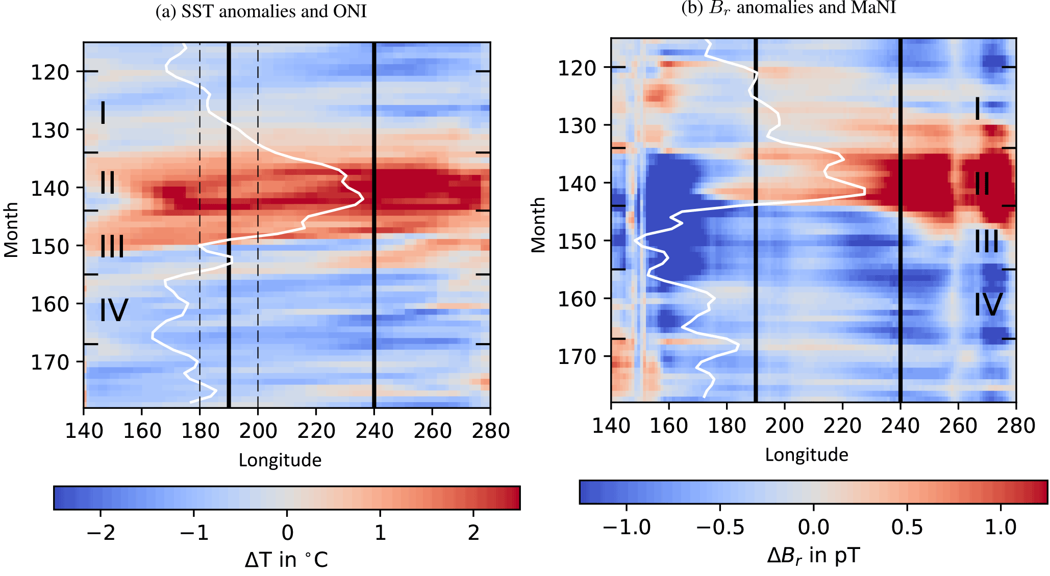
Figure 2 Hovmöller plots of sea surface temperature anomalies (a) and B_r anomalies (b) averaged from 5^∘ S to 5^∘ N. The time interval shows the strongest ENSO cycle cf. Fig. 1. Vertical black lines enclose the Niño 3.4 region used to calculate ONI and MaNI. The solid white lines represent the indices derived from the individual anomalies centred on 170^∘ E (20^∘ of longitude corresponds to 1 ^∘C a and 0.4 pT b). The dashed lines represent the ONI thresholds for El Niño/La Niña of ±5 ^∘C (a).

The analysis of the cross-correlation of the two indices (embedded plot in Fig. 1) shows a MaNI lead of 4 months over the ONI. Accounting for this lead, the correlation of both time series increases to 0.72.

Since in our setup (see Sect. 2.2) the only time-variable contribution to B_r is the seawater conductivity σ, we conclude that in the Niño 3.4 region subsurface anomalies of σ, caused by anomalies in S and T, are leading SST anomalies.

Current magnetometers like the absolute scalar magnetometers of the Swarm mission with accuracy of < 45 pT and a sensitivity of 1 pT $/\sqrt{\mathrm{Hz}}$ (Jager et al., 2010) are able to resolve the global structure of the oceanic tidally induced radial magnetic field. To be able to observe the presented variations an increase magnetometer precision of several orders of magnitude down to the femtotesla scale is necessary.

Given the task at hand, two of the most promising magnetometer technologies are superconducting quantum interference devices (SQUIDs) and spin-exchange relaxation free (SERF) atomic magnetometer. SQUIDs, which are also used in technologies such as MRI or magnetoencephalography to detect biomagnetic fields, have achieved noise levels as low as 0.3 fT $/\sqrt{\mathrm{Hz}}$ (Schmelz et al., 2011). Also, Kominis et al. (2003) have presented an SERF-based atomic magnetometer with a measurement volume 1800 cm³ and a sensitivity of 0.54 fT $/\sqrt{\mathrm{Hz}}$. Additionally, they have shown that the theoretical achievable fundamental sensitivity is below 0.01 fT $/\sqrt{\mathrm{Hz}}$. These exciting improvements however are still in the laboratory phase where disturbing influences can be controlled way better than under field conditions. SQUID-based geomagnetic field sensors have been reported to have reached sensitivities of 6 fT $/\sqrt{\mathrm{Hz}}$ (Schönau et al., 2013). Challenges in the calibration of the sensor however limited the absolute accuracy to 0.3 nT.

Since necessary magnetometer observations are not limited to satellite measurements, but could also originate from measuring stations deployed at ocean bottom or an array of moored buoys, there are several options to overcome the present obstacles in measurability. Given the advancements in magnetic field sensor technology, it is reasonable to assume that ENSO-induced B_r anomalies investigated in this study might become detectable in the intermediate to far future. Even more so considering that the absolute accuracy is less important than the precision in our case, since we investigate periodical variations of the geomagnetic field. Also, not only are the periodic oceanic tidally induced radial magnetic field signals easily extracted from geomagnetic field observations of multiple contributing sources; additionally the error decreases by $n^{-\mathrm{1}/\mathrm{2}}$, where n equals the number of observations in a time series.

3.2 Spatio-temporal anomaly development

Temporal and spatial development of SST and B_r anomalies of the strongest ENSO cycle of the time series (grey shaded interval in Fig. 1) are displayed as Hovmöller plots in Fig. 2.

Considering the large-scale changes in ocean temperature and salinity due to ENSO, large ocean conductance and consequently considerable B_r anomalies are to be expected. In fact, the range in MaNI is approximately 3 times the range of the seasonal cycle in the same region (cf. Sect. 3.1). However, the changes of these surface processes are small compared to the total conductance, integrated from ocean bottom to sea surface. Hence, the anomalies in B_r considered here amount to less than 1 % of the total signal.

The presence of the geomagnetic equator in the equatorial Pacific region creates an additional hindrance. The vertical component of B_Earth, the geomagnetic field component inducing B_r, undergoes a change of sign here and vanishes. Consequently, B_r vanishes at the geomagnetic equator and expresses small values in its immediate proximity.

Also, the M2 tidal flow is not homogeneously distributed throughout the equatorial Pacific. Local maxima and minima in the tidal flow cause an additional modulation of the radial tidally induced magnetic field.

To diminish these disturbing influences, B_r anomalies have been spatially averaged from 5^∘ S to 5^∘ N. SST anomalies have also been averaged over that range for comparability of both images. Vertical lines in Fig. 2b at ≈ 260^∘ W are remaining artefacts caused by the southward dip in the geomagnetic equator in that region.

The comparison of Fig. 2a, b shows that positive B_r anomalies emerge almost a year before they form in SST (phase I). The same is found for negative B_r anomalies. They emerge months before positive SST anomalies recede and mark the end of El Niño (phase III). Although the presented image shows only the spatio-temporal progression of the strongest cycle of an El Niño followed by a La Niña, these findings are comparable for the other regular ENSO cycles (not shown).

With the beginning of phase I, a positive B_r anomaly is found west of the Niño 3.4 region, while at sea surface cold or neutral conditions are found. Then positive B_r anomalies travel through the Niño 3.4 region eastwards. They are probably caused by equatorial Kelvin waves which are known to precede the onset of El Niño (Harrison and Schopf, 1984). Kelvin waves deepen the thermocline and increase the amount of warm seawater in the water column. A rise in seawater conductance, the depth-integrated seawater conductivity, is the consequence. SST anomalies have not yet formed during this phase. An intensification of positive B_r anomalies on the South American west coast is observed with the arrival of the Kelvin waves several months before the ONI-defined start of El Niño. This can be explained by the deepening of the thermocline (Wang and Picaut, 2013) and the corresponding anomalous increase of warm water in the upper ocean.

During phase II, El Niño effects become apparent at the sea surface. Here, the typical El Niño weakening of trade winds leads to changes of wind patterns in the Walker circulation and alters the equatorial ocean current system (McPhaden, 1999). As a consequence, the warm water of the western Pacific warm pool flows eastward and leads to an increase and westward expansion of SST anomalies at the Peruvian coast. The eastward migrating warm water causes a thermocline shallowing in the western warm pool and a simultaneous deepening of the thermocline at the Peruvian coast. This leads to negative (positive) B_r anomalies west (east) of the Niño 3.4 region reaching local amplitudes of −6 (3 pT) when El Niño is fully developed. The general agreement of ONI and MaNI during this phase and the co-occurring maxima of both indices show that sea surface and subsurface dynamics exhibit similar behaviour under the influence of a common cause.

The beginning of phase III is marked by an eastward expansion of the western negative B_r anomaly that formed during phase II. The effects of El Niño, in form of warm SST anomalies, are still present for several months. Subsurface processes, however, cause an early decrease in B_r anomalies and consequently in MaNI. The eastern positive B_r anomaly recedes and a negative anomaly forms months before the onset of La Niña becomes apparent in ONI.

Phase IV marks the beginning of La Niña at sea surface. The Walker circulation returns to normal conditions and the westward direction of the equatorial ocean current is re-established. Hence, the eastern thermocline shallows due to upwelling of cold water and warm surface water is transported to the western warm pool. Westward-travelling SST and B_r anomalies result in the increased agreement of ONI and MaNI.

With the end of phase IV a new cycle starts. The build-up of positive B_r anomalies, as described in phase I, can be observed towards the end of the plotted time interval.

The analysis shows that the identified lead in the MaNI is not just a mere forward shift of the signals but a combined result of multiple effects. We found that it is a combination of early signs for the onset of the El Niño probably caused by eastward-travelling Kelvin waves and a decrease in the magnetic signal months before the actual end of El Niño due to a shallowing of the thermocline. Consequently, the cycle of B_r anomalies and SST anomalies are phase shifted.

3.3 Cross-correlation ONI and conductance

The findings obtained from calculating the cross-correlation between the oceanic conductance and the ONI at each grid point are summarized in Fig. 3.

In Fig. 3a, the maximum conductance anomaly of the time series at each grid point is shown. The magnitude of conductance anomalies is linked to the magnitude of relative B_r changes. The largest signals are therefore evident in the western warm pool and at the west coast of South America. In these regions, the thermocline undergoes the largest relative changes as a result of ENSO. We also find that the conductance anomalies are elevated in a small band throughout the whole equatorial region. This region is the passage way of the equatorial Kelvin waves which vary the thermocline depth.

In Fig. 3b, the maximum absolute correlation is plotted. Largest values are found east of the Niño 3.4 region. The correlation, the conductance and the ONI decrease westwards in a tongue-shaped pattern, like the typical SST anomalies of El Niño and La Niña.

Figure 3 Cross-correlation analysis between the ONI and the conductance (σ_int) at each grid point: maximum absolute conductance anomaly (a), absolute maximum correlation, the peak value of the cross-correlation (b), corresponding lead/lag to the absolute maximum correlation (c). The solid rectangle shows the location of the Niño 3.4 region, the dashed rectangle shows the location of an updated MaNI (5^∘ N–5^∘ S, 150–170^∘ W).

Figure 3c shows the lag between the ONI and the conductance. The lead in conductance increases in a tongue-shaped pattern originating from the South American west coast. Since the Kelvin waves travel eastwards, an increase in the lead towards their origin is a logic consequence.

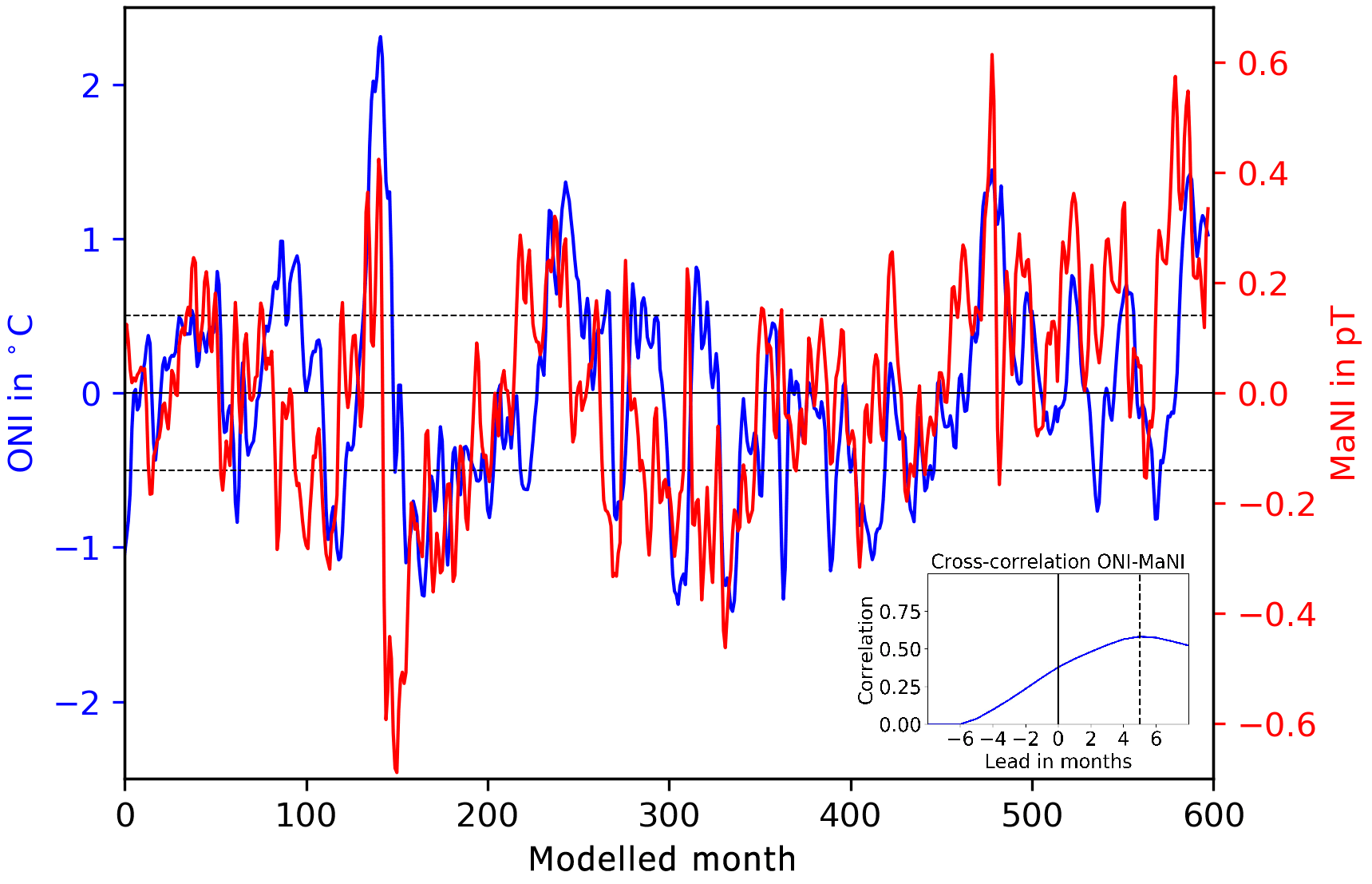
Figure 4 Comparison of time series of ONI (blue) and updated MaNI (red). Anomaly strength and correlation are reduced, while the lead increases.

For the Niño 3.4 region (solid rectangles in Fig. 3), we find the same characteristics as for the analysis in Sect. 3.1. The maximum absolute correlation of the whole region ranges from ≈ 0.7 to ≈ 0.8 (Fig. 3b). The lead distribution in the area is not uniform. A large part of the western half leads by 5 months and decreases eastward to 2 months. The area-averaged B_r anomalies of the MaNI therefore produce a signal that leads statistically by 4 months with a correlation between 0.7 and 0.8.

3.4 Qualitative application of findings

The robustness of our findings is tested with a reanalysis of the correlation between ONI and MaNI using an updated averaging region for the MaNI. The new region is located at 5^∘ N–5^∘ S, 150^∘–170^∘ W. It keeps the poleward extent of ±5^∘, which accounts for the presence of the geomagnetic equator in order to assure an adequate averaging. The eastern boundary is shifted westwards to increase the lead in magnetic field anomalies over SST anomalies (see Fig. 3c). The westward shift is constrained by the maximum correlation found in Fig. 3b. A recalculation of the MaNI within the updated region is shown in Fig. 4.

The reanalysis shows an overall decrease in correlation between the two time series. For a lag of 0 months, the correlation is decreased from 0.63 to 0.38. The maximum correlation is decreased from 0.72 to 0.58, while the lead is increased from 4 to 5 months. Additionally, the range of the updated MaNI shrank from −0.84 to 0.82 pT to a range of −0.69 to 0.61 pT. These results are in agreement with the previous findings of Sect. 3.3. We conclude that the lead in MaNI found in Sect. 3.1 and 3.2 is caused by the lead in conductance anomalies found in Sect. 3.3.

Correlation and cross-correlation are methods for determining the linearity of the relationship between two variables. ENSO is the defining influence on the progression of ONI and MaNI. However, we found that the processes contributing to ENSO cause differing developments in sea surface and subsurface dynamics. Consequently, the decrease in correlation should be viewed as an increase in information gained from the perspectives of SST and B_r anomalies on the same phenomenon.

4 Conclusions

Seawater temperature and salinity altering processes are known to be integrated in the electromagnetic oceanic tidal signals from bottom to surface. We investigated whether the tidally induced magnetic fields could be used as an indicator for the El Niño–Southern Oscillation.

We used a coupled ocean–atmosphere general circulation model to simulate 50 years of monthly mean seawater temperature, salinity and pressure distributions. The properties were used to calculate the tidal electromagnetic signals for each month.

We analysed the relationship between electromagnetic signals and ENSO by comparing two ENSO indices. These indices, calculated in the Niño 3.4 region, are the ONI, based on SST anomalies, and the proposed Magnetic Niño Index (MaNI), based on anomalies in the tidal magnetic field. We show that both indices are highly correlated and MaNI leads the ONI by 4 months.

In order to explain this lead, the spatial and temporal evolution of B_r anomalies was analysed and compared with the evolution of SST anomalies. We found the lead to be explainable with eastward-travelling equatorial Kelvin waves. They are known to precede the development of typical ENSO SST anomalies. They also increase the thermocline depth in the eastern Pacific ocean. In consequence, the electric conductance of the upper ocean is elevated which results in a stronger tidal magnetic field.

Based on these results, we analysed the relationship between the ONI and equatorial Pacific conductance anomalies. The spatial distributions of correlation, lead and signal strength were in good agreement with the found MaNI characteristics. We showed that correlation of conductance anomalies and ONI increases eastward, while the lead over the ONI increases westward.

With these findings we updated the averaging region for the recalculation of the MaNI. With the new index, our interpretation was confirmed and the lead in MaNI was increased to 5 months. At the same time, signal strength and correlation were reduced. The decrease in correlation is interpreted as a gain in information about subsurface dynamics of ENSO rather than a loss in information about ENSO itself. Traditionally, researchers have focused on sea surface dynamics for signs of El Niño. The latest research, however, shows that subsurface dynamics play a crucial role in the build-up phase and the decline of El Niño. An increased focus on subsurface processes is therefore necessary to understand ENSO completely.

With the modelled tidal magnetic field anomalies being too small to be detectable with contemporary measuring methods, the presented results are not applicable at present times. However, magnetometer sensitivity under laboratory conditions have reached noise levels several orders of magnitude below the necessary detection threshold for the presented B_r anomalies. Consequently, a detection of the analysed signals is at least theoretical possible, even though it might be improbable due to technical limitations in field measurements.

In summary, our study shows that the dynamic of tidally induced radial magnetic field anomalies contains information for an early awareness of developing anomalous warm and cold ENSO conditions. Given that the substantial improvements in observation techniques lead to observations of these signals, this could be used to improve current ENSO warning systems and mitigate its negative impacts.