the Creative Commons Attribution 3.0 License.
the Creative Commons Attribution 3.0 License.
Biological data assimilation for parameter estimation of a phytoplankton functional type model for the western North Pacific
Yasuhiro Hoshiba
Takafumi Hirata
Masahito Shigemitsu
Hideyuki Nakano
Taketo Hashioka
Yoshio Masuda
Yasuhiro Yamanaka
Ecosystem models are used to understand ecosystem dynamics and ocean biogeochemical cycles and require optimum physiological parameters to best represent biological behaviours. These physiological parameters are often tuned up empirically, while ecosystem models have evolved to increase the number of physiological parameters. We developed a three-dimensional (3-D) lower-trophic-level marine ecosystem model known as the Nitrogen, Silicon and Iron regulated Marine Ecosystem Model (NSI-MEM) and employed biological data assimilation using a micro-genetic algorithm to estimate 23 physiological parameters for two phytoplankton functional types in the western North Pacific. The estimation of the parameters was based on a one-dimensional simulation that referenced satellite data for constraining the physiological parameters. The 3-D NSI-MEM optimized by the data assimilation improved the timing of a modelled plankton bloom in the subarctic and subtropical regions compared to the model without data assimilation. Furthermore, the model was able to improve not only surface concentrations of phytoplankton but also their subsurface maximum concentrations. Our results showed that surface data assimilation of physiological parameters from two contrasting observatory stations benefits the representation of vertical plankton distribution in the western North Pacific.
- Article
(11706 KB) - Full-text XML
- BibTeX
- EndNote


The western North Pacific (WNP) region is a high-nutrient, low-chlorophyll (HNLC) region where biological productivity is lower than expected for the prevailing surface macronutrient conditions. There are both the Western Subarctic Gyre and Subtropical Gyre, comprising the Oyashio and the Kuroshio, respectively (Fig. 1a). Between the gyres (i.e. the Kuroshio–Oyashio transition region), horizontal gradients of temperature and phytoplankton concentration in the surface water are generally large due to meanders in the Kuroshio extension jet and mesoscale eddy activity (Qiu and Chen, 2010; Itoh et al., 2015). The relatively low productivity in the HNLC region is due to low dissolved iron concentrations (e.g. Tsuda et al., 2003) because iron is one of the essential micronutrients for many phytoplankton species. The source of iron for the WNP region is not only from airborne dust but also from iron transported in the intermediate water from the Sea of Okhotsk to the Oyashio region (Nishioka et al., 2011). Since the WNP region exhibits many complex physical and biogeochemical characteristics as referred to above, it is difficult even for state-of-the-art eddy-resolving models to reproduce them.
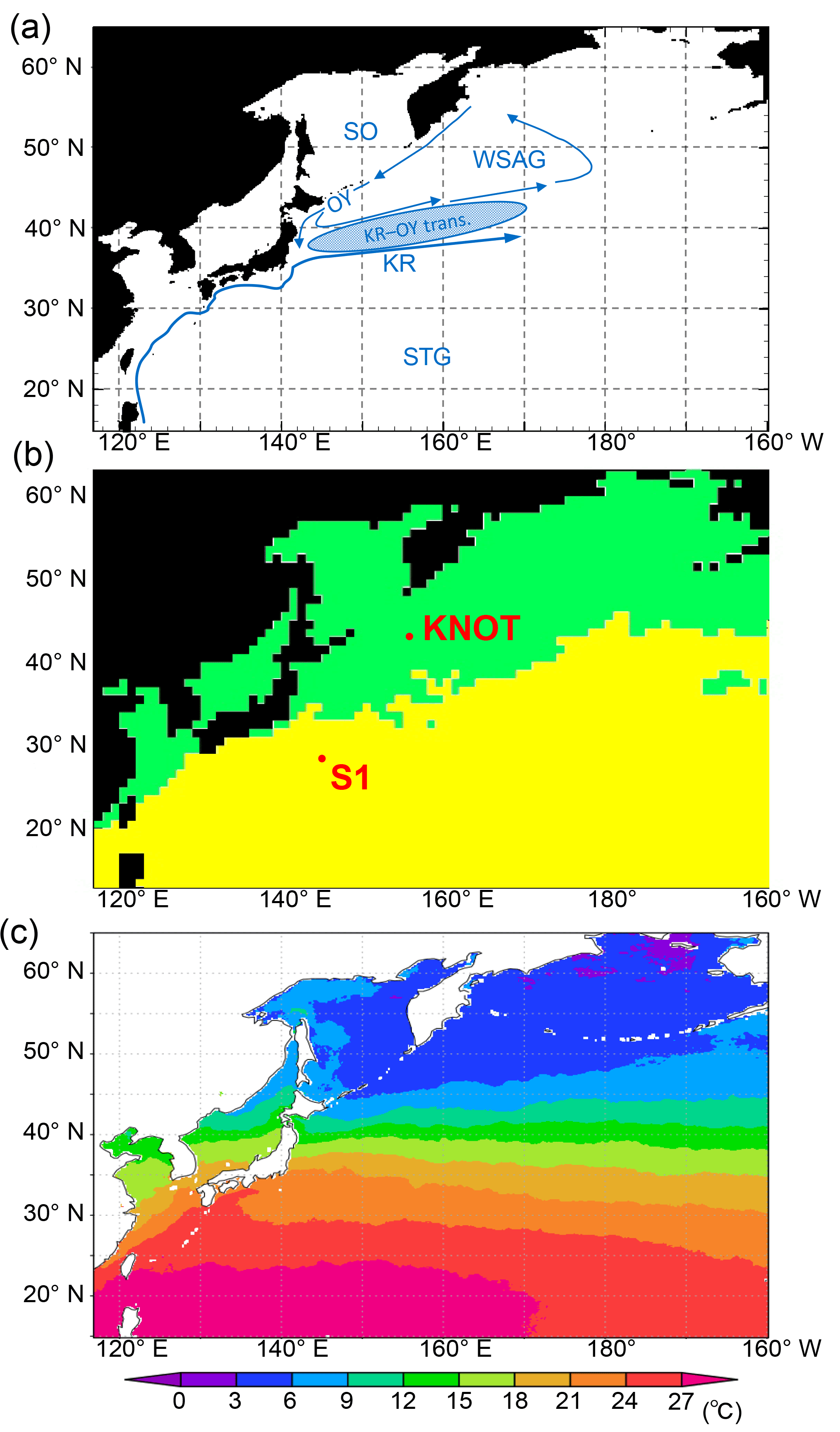
Figure 1(a) Model domain in the WNP region of the 3-D NSI-MEM. Blue arrows and symbols depict a schematic representation of the main circulation features in the WNP (KR: Kuroshio; OY: Oyashio; KR-OY trans.: the Kuroshio–Oyashio transition region; STG: Subtropical Gyre region; WSAG: Western Subarctic Gyre; and SO: the Sea of Okhotsk). (b) Two classified provinces (subarctic and subtropical regions) based on the dominant phytoplankton species and nutrient limitations by Hashioka et al. (2018). Different ecosystem parameters (Table 2) are set for each province in the simulation. (c) Annual mean SST of satellite data used for simulation of SST-dependent physiological parameters (SST-dependent case).
Processes of growth, decay, and interaction by plankton are critical to understanding the oceanic biogeochemical cycles and the lower-trophic-level (LTL) marine ecosystems. There are many LTL marine ecosystem models ranging from simple nutrient, phytoplankton, and zooplankton models to more complicated models including carbon, oxygen, silicate, and iron cycles, and so forth (e.g. Fasham et al., 1990; Edwards and Brindley, 1996; Lancelot et al., 2000; Yamanaka et al., 2004; Blauw et al., 2009). Coupling LTL marine ecosystem models to ocean general circulation models (OGCMs) and Earth system models enables three-dimensional (3-D) quantitative descriptions of the ecosystem and its temporally fine variability (e.g. Aumont and Bopp, 2006; Follows et al., 2007; Buitenhuis et al., 2010; Sumata et al., 2010; Hoshiba and Yamanaka, 2016).
Physiological parameters are usually fixed in the models on the basis of local estimations and applied homogeneously to a basin-scaled ocean, although the values of physiological parameters should depend on the environments of regions. Moreover, physiological parameters have often been tuned up empirically and arbitrarily. The fact that the number of parameters increases with prognostic and diagnostic variables makes it more difficult to tune them. In order to reproduce observed data such as spatial distribution of phytoplankton biomass and timing of a plankton bloom, it is required to reasonably estimate the physiological parameters.
In previous studies using LTL marine ecosystem models, various approaches for data assimilation were introduced as methods of estimating optimal physiological parameters (e.g. Kuroda and Kishi, 2004; Fiechter et al., 2013; Toyoda et al., 2013; Xiao and Friedrichs, 2014). Shigemitsu et al. (2012) applied a unique assimilative approach to an LTL marine ecosystem model, using a micro-genetic algorithm (μ-GA) (Krishnakumar, 1990). For the western subarctic Pacific, they showed that the μ-GA worked well in the one-dimensional (1-D) Nitrogen, Silicon and Iron regulated Marine Ecosystem Model (NSI-MEM: Fig. 2), which was based on NEMURO (North Pacific Ecosystem Model for Understanding Regional Oceanography; Kishi et al., 2007) but differed in the following points: (1) the introduction of an iron cycle, including dissolved and particulate iron, whereby the dissolved iron explicitly regulates phytoplankton photosynthesis; (2) adoption of physiologically more consistent optimal nutrient-uptake (OU) kinetics (Smith et al., 2009) instead of the Michaelis–Menten equation (Michaelis et al., 2011); and (3) the division of detritus into two types of small and large sizes that exhibit different sinking rates.
Our objective is to improve simulation of the LTL ecosystem in the WNP region by further introducing (1) a physical field from an eddy-resolving OGCM with a horizontal resolution of 0.1∘ and (2) an assimilated physiological parameter estimation for two different phytoplankton groups. The details of the model and μ-GA settings are described in Sect. 2. We compare the simulation results with and without the parameter optimization to observed data and confirm the effects of changing parameters in Sect. 3. We mainly focused on the seasonal variations in phytoplankton in the pelagic region. Finally, the results are summarized in Sect. 4.
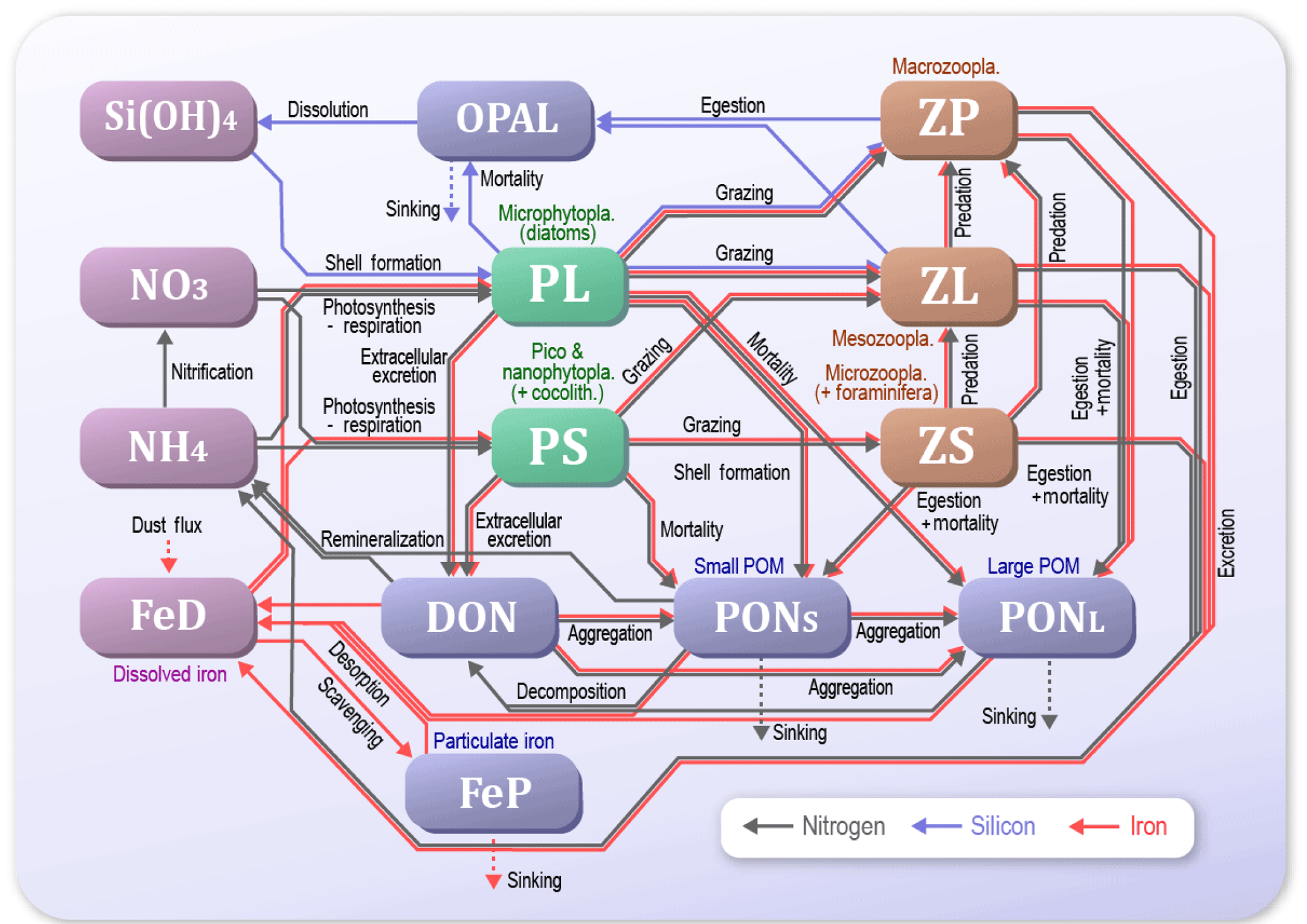
Figure 2Schematic view of the NSI-MEM interactions among the 14 components. Green boxes and brown boxes indicate phytoplankton and zooplankton, respectively. Blue boxes are particulate or dissolved matter. Violet boxes show nutrients or essential micronutrients.
2.1 Three-dimensional NSI-MEM
We used the marine ecosystem model, NSI-MEM, which includes two phytoplankton functional types (PFTs), namely non-diatom small phytoplankton (PS) and large phytoplankton representing diatoms (PL) (Fig. 2). In order to run the NSI-MEM in three-dimensional space, we used a physical field obtained from the Meteorological Research Institute Multivariate Ocean Variational Estimation for the WNP region (MOVE-WNP) (Usui et al., 2006). The MOVE-WNP system is composed of the OGCM (the Meteorological Research Institute community ocean model) and a multivariate 3-D variational (3-D VAR) analysis scheme. The 3-D VAR method adds some increments to only the temperature and salinity fields. The increments are derived so as to minimize the misfits between the model and observations of temperature, salinity, and sea surface dynamic height (Fujii and Kamachi, 2003). The dynamical fields such as flow speed and sea surface height are not directly modified by the 3-D VAR method (i.e. the physical field holds water mass conservation, which is necessary to run the ecosystem model with a consistent manner).
The model domain extends from 15 to 65∘ N and 117∘ E to 160∘ W in the WNP region, with a grid spacing of 1/10∘ × 1/10∘ around Japan and 1/6∘ to the north of 50∘ N and to the east of 160∘ E (Fig. 1a). There are 54 vertical levels with layer thicknesses increasing from 1 m at the surface to 600 m at the bottom. The model was forced by factors including surface wind, heat flux, and freshwater flux. The details of the surface forcing are presented by Tsujino et al. (2011). Shortwave radiation input and dust flux were the same as those of a global climate model (Model for Interdisciplinary Research on Climate, MIROC; Watanabe et al., 2011). A part of the dust flux (3.5 %; Shigemitsu et al., 2012) was regarded as iron dust, and 1 % of the iron dust was assumed to dissolve into the sea surface (Parekh et al., 2004). The other iron dust was transported to the lower layers and dissolved, which was the same process as shown in Shigemitsu et al. (2012). River run-off as a freshwater supply was from CORE v. 2 forcing (Large and Yeager, 2009), in which the river source had the nitrate concentration value of 29 µmol L−1 (Cunha et al., 2007) and the silicate concentration value of 102 µmol L−1 adjusted in the range between Si ∕ N = 0.2 and 4.3 (Jickells, 1998). Nitrate and silicate sources were only rivers, and iron supply was only from the dust in the model setting. In order to buffer artificial high concentrations near the side edge of the model domain, nutrients near the southern and eastern boundaries of the model domain were only restored for 43 min to 3.6 h to the values provided by the Meteorological Research Institute Community Ocean Model (MEM-MRI.COM) participating in MARine Ecosystem Model Intercomparison Project (https://pft.ees.hokudai.ac.jp/maremip/data/MAREMIPh_var_list.html, last access: 28 May 2018). The physical field used in our ecosystem model had already been confirmed to reproduce realistic salinity, velocity, and temperature fields in a previous study (Usui et al., 2006). Using a physical 1-day averaged field, we ran the NSI-MEM to simulate the years between 1985 and 1998.
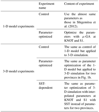
We divided the model domain into two provinces (green and yellow regions in Fig. 1b) using the following province map instead of maps divided by latitude–longitude lines as in previous studies (e.g. Longhurst, 1995; Toyoda et al., 2013). The province map is based on the dominant phytoplankton species and nutrient limitations (Hashioka et al., 2018) and sets different ecosystem parameters (see details in Sect. 2.3) for each province (hereafter, “parameter-optimized case: OPT”; Table 1). For each province, the respective parameters estimated by the μ-GA and the 1-D NSI-MEM were employed for those in the 3-D NSI-MEM. A large gap in a horizontal distribution of phytoplankton can appear on the boundary of the two provinces in Fig. 1b due to a gap in the different parameter sets at the boundary. In order to smooth the gap in parameter values at the boundary between the two provinces in Fig. 1b, the parameters were varied as a function of the sea surface temperature (SST) annually averaged for 1998 (Fig. 1c) for our “SST-dependent case: SST-OPT” (Table 1). While phytoplankton fluctuate with not only SST but also other surrounding conditions such as nutrient abundance in the real ocean (Smith and Yamanaka, 2007; Smith et al., 2009), we chose SST because μ-GA optimization is conducted for physiological parameters of both phytoplankton and zooplankton (Table 2) and the SST directly affects physiology of both of them whereas nutrients and light were essentially related to phytoplankton. The parameters were interpolated and extrapolated according to the following equation:
where P(x), PSt. S1, and PSt. KNOT are ecosystem parameters for a point (x), the station S1, and the station KNOT, respectively. KNOT and S1 are typical observational points in the subarctic and subtropical regions (green- and yellow-coloured areas in Fig. 1b, respectively). We also conducted model experiments with the parameters similar to those in Shigemitsu et al. (2012) for the whole domain (hereafter “control case: CTRL”, Table 1). The parameters of all the 3-D experimental cases, shown in Table 1, were not changed either vertically or temporally. In the parameter-optimized and SST-dependent cases, the parameters were the same as the control case from 1 January 1985 to 31 December 1996. During the next 1 year (1997), the simulations were spun-up with the optimized or SST-dependent parameters. Then, simulation results on 1 January 1998 were used as initial conditions for the 1998 simulations. The parameter values used in the control case were not changed during the 1985–1998 period. The simulation results for the last year (i.e. 1998) were analysed and compared to observational data of 1998.
2.2 Satellite and in situ data
Global satellite data for 1998 for phytoplankton (i.e. chlorophyll a) were obtained from the Ocean Colour Climate Change Initiative, European Space Agency, available online at http://www.esa-oceancolour-cci.org/ (last access: 28 May 2018), which utilized the data archives of ESA's MERIS/ENVISAT and NASA's SeaWiFS/SeaStar and Aqua/MODIS. The global satellite data, which have the horizontal resolution of 0.042∘, were linearly interpolated to the grid (size 1/10 and 1/6∘) in the model domain (Fig. 1a), and the nitrogen-converted concentrations of both PL and PS were estimated based on a satellite PFT algorithm (Hirata et al., 2011). The μ-GA cost function was defined from the 1998 monthly averaged PL and PS concentrations. The satellite data of daily temporal resolution were not useful due to many regions with missing values. Therefore, we discuss the results of the monthly scale in the present study.
Satellite data of the 1998 mean SST (horizontal grids of 0.088∘) from the AVHRR-Pathfinder project (http://www.nodc.noaa.gov/SatelliteData/pathfinder4km/, last access: 28 May 2018) were also used to conduct our SST-dependent case study using the same interpolation procedure as above. The data were linearly interpolated between satellite and model grids, which could introduce some uncertainty to the satellite data. In addition, the use of the global chlorophyll data in the regional study for the WNP region could be another error source of the observational data: the previous study (Gregg and Casey, 2004) showed that the regional root mean square log % errors of the satellite data ranged from 24.7 to 31.6 in the North Pacific.
To validate the vertical distribution of the model results, we utilized in situ data of phytoplankton and nutrients in 1998 along the 165∘ E section taken from the World Ocean Database 2013 (https://www.nodc.noaa.gov/OC5/WOD13/, last access: 28 May 2018), and at KNOT (44∘ N, 155∘ E) obtained from the website (http://www.mirc.jha.or.jp/CREST/KNOT/, last access: 28 May 2018) (Tsurushima et al., 2002).
2.3 One-dimensional NSI-MEM process
The 1-D NSI-MEM used in Shigemitsu et al. (2012) was employed as an emulator to determine the optimal set of ecosystem parameters at KNOT (44∘ N, 155∘ E) and S1 (30∘ N, 145∘ E), respectively. We modified the 1-D NSI-MEM of Shigemitsu et al. (2012) by increasing the number of vertical layers to 54 and introducing the vertical advection of the 3-D simulation. Of 107 physiological parameters in the NSI-MEM, 23 were selected, as shown in Table 2, which were responsible for PL and PS biomass relevant to the photosynthesis and the grazing of zooplankton. In the previous study, Yoshie et al. (2007) also suggested that some parameters in the 23 parameters were relatively influential on PS and PL, more than the other physiological parameters such as those for the sinking process of particulate matters (PON, OPAL in Fig. 2). The other parameters of the NSI-MEM were the same as those in the control case. The initial (1 January 1998) and boundary conditions during the integration period were applied from those in the 3-D model.
2.4 μ-GA implementation
The μ-GA procedure requires a cost function. To define the cost function (Eq. 2), satellite PFT data were used as reference values for the μ-GA because satellite data have higher temporal and spatial resolution than in situ data. The μ-GA procedure works in such a way that a parameter set of the lowest cost is retained, and then a new parameter set is determined by crossover and mutation methods using the retained set. An optimized parameter set is finally provided by repeating the process multiple times.
Running the 1-D NSI-MEM with the μ-GA, the 23 optimal parameters were obtained through the following process.
-
Step 0. Define a range of parameter values (Table 2) based on previous studies (e.g. Jiang et al., 2003; Fujii et al., 2005; Yoshie et al., 2007) and prepare 23 model runs with the same number of estimated parameters before running the μ-GA.
-
Step 1. Generate 23 initial random parameter sets using the μ-GA.
-
Step 2. Evaluate the 23 model runs with the different parameter sets using the following cost function:
where mi is the modelled monthly mean of phytoplankton type i(i=1 for PL and 2 for PS) and di is the monthly satellite data of type i. The index j denotes the number of months (Ni) for which satellite data of type i exist. The assigned weights for PL and PS were the same low value (σPL = 0.1 µmol L−1 and σPS= 0.1 µmol l−1) as some weights used in Shigemitsu et al. (2012).
-
Step 3. Determine the best parameter set and carry it forward to the next model run (or the next “generation”) (elitist strategy).
-
Step 4. Choose the remaining 22 sets for re-determination of the best parameter sets (or “reproduction”) based on a deterministic tournament selection strategy (the best parameter set that gave the highest model performance in Step 3 also competes for its copy in the reproduction). In the tournament selection strategy, the parameter sets are grouped randomly and adjacent pairs are made to compete. Apply crossover to the winning pairs and generate new parameter sets for the final 22 parameter sets. Two copies of the same set mating for the next generation should be avoided.
-
Step 5. If the difference between the maximum and minimum cost function values of the model runs becomes smaller than a threshold value, renew all the parameter sets randomly except for the best-performed set for efficiently escaping from a local solution; the cost function may have local minimums.
-
Step 6. Repeat the procedure from Step 2 to Step 5 until the best parameter set is well converged within 2000 generations (times) in the present study.
The 1-D NSI-MEM was used as an emulator to determine ecosystem parameters through the process described above, and the parameter sets assimilated by the 1-D model with the μ-GA at KNOT and S1 were applied to the 3-D simulations, which were conducted as the parameter-optimized case and the SST-dependent case in Table 1.
3.1 One-dimensional model
The 1-D NSI-MEM was employed to determine ecosystem parameters for the 3-D-model simulation. The 1-D simulation results (Fig. 3) of the parameter-optimized case (blue dashed lines) are clearly closer to satellite data (solid lines) than those of the control case (orange dashed lines). The cost-function values estimated by the 1-D simulations in the OPT, 1.61 and 0.17 at KNOT and S1, are also about 8 and 6 times smaller than those in the CTRL, 13.55 and 1.11, respectively (not shown).
The total biomass (PL + PS) at KNOT in the subarctic region is larger than that at S1 in the subtropical region. The PS biomass (Fig. 3a, c) is larger than the PL biomass (Fig. 3b, d) at both KNOT and S1. As for the relative ratio of PL to the total biomass, the relative ratio at KNOT is larger than that at S1. These results are consistent with the general understanding that biomass in the subarctic region is larger than that in the subtropical region, and that the ratio of PL to the total biomass in the subarctic region is also larger than that in the subtropical region.
Seasonal variations in the OPT for the two stations simulated with the satellite data assimilation are also improved drastically in comparison to the CTRL. The seasonal variations in PS and PL at KNOT (Fig. 3a, b) in the OPT have relatively high concentrations with a winter peak of 630 and 130 µmol N m−3, respectively. In the CTRL of PS, however, there is a spring (May) peak of 180 µmol N m−3, and the PL concentration remains low through the year. At S1, the PS seasonal variations tend towards a high concentration in winter and low concentration from summer to autumn in the OPT, while the PS concentration, in the CTRL, in summer to autumn is higher than that in winter. The PL concentrations of the two model cases are almost zero, and that of the satellite is also remarkably small (< 21.5 µmol N m−3). The parameter-optimization process with the 1-D model works well in terms of the seasonal variations in surface phytoplankton.
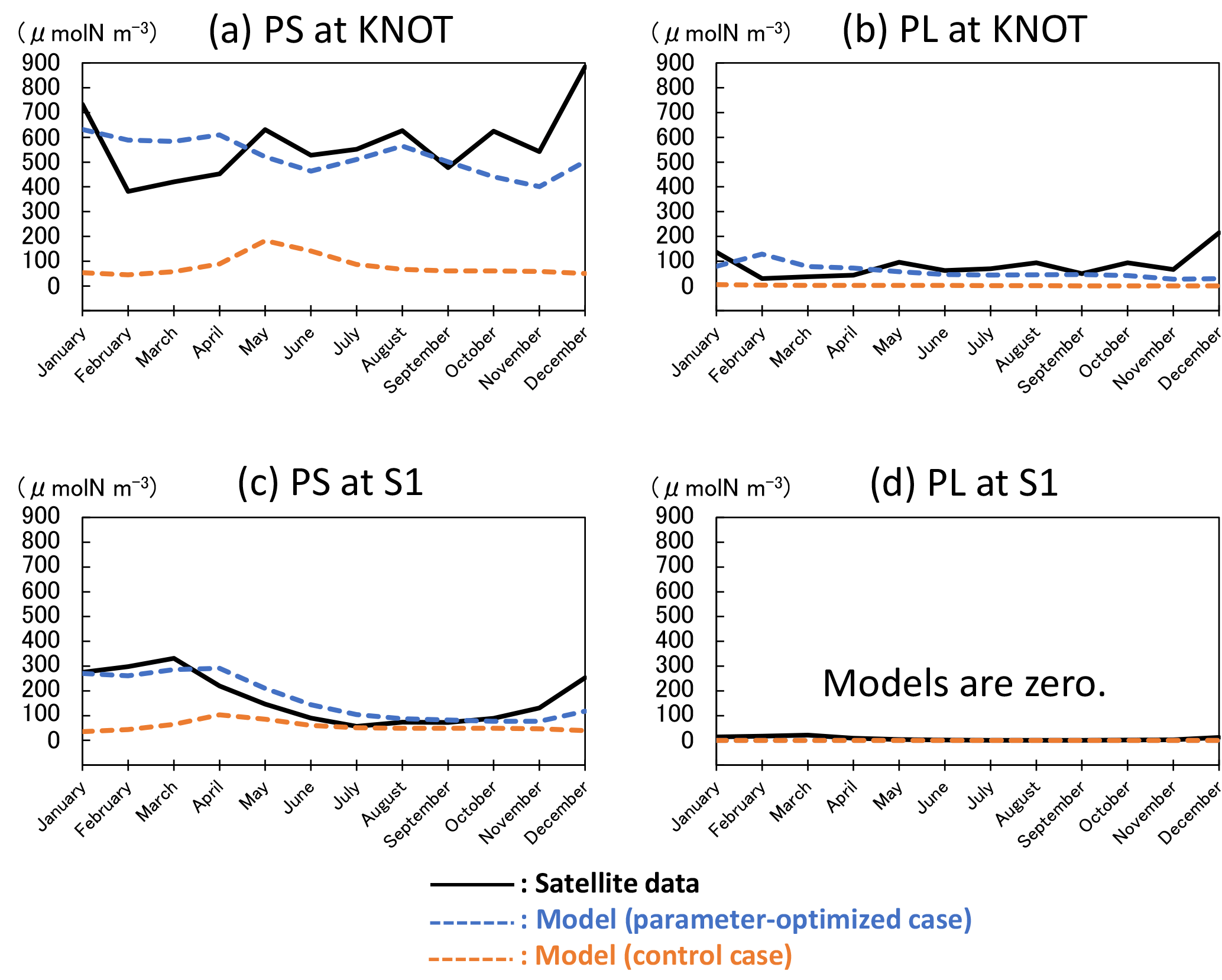
Figure 3Seasonal variations in surface phytoplankton (PS: small phytoplankton and PL: large phytoplankton) biomass in the 1-D NSI-MEM and satellite data at KNOT and S1 shown as typical observational points of the subarctic and the subtropical regions, respectively. (a) PS at KNOT, (b) PL at KNOT, (c) PS at S1, and (d) PL at S1, where the concentrations of the two model cases are almost zero, and that of the satellite is also remarkably small. The unit conversion between the simulation data (mol N m−3) and the satellite data (g chl a m−3) is referred to as the nitrogen ∕ chlorophyll ratio of PL = 1 : 1.59 and PS = 1 : 0.636 (Shigemitsu et al., 2012). The same conversion of nitrogen to chlorophyll is used in Figs. 4, 6, 8, and 10.
3.2 Three-dimensional model
The parameter set estimated by the 1-D model at KNOT and S1 was applied to the 3-D simulation (Fig. 4). The seasonal features in the 3-D simulation are generally similar to those seen in the 1-D simulation (i.e. relatively small seasonal variations in PS biomass in the subarctic region and a relatively high winter biomass in the OPT, compared to the CTRL). At KNOT, for instance, there is the smaller difference between the high (575 µmol N m−3 in January) and low (398 µmol N m−3 in October) concentrations in the OPT than the high (568 µmol N m−3 in July) and low (59 µmol N m−3 in January) concentrations in the CTRL. The PL biomass features are also similar to those of the PS biomass mentioned above, except that the PL biomass is lower in the subtropical region in the OPT than in the CTRL. Seasonal peaks of PS and PL biomass also have the same features as those in the 1-D simulations (i.e. the PS bloom in the OPT occurs from winter to spring (Fig. 4c, g), but that in the CTRL occurs in summer (Fig. 4b). The SST-OPT results are discussed later in Sect. 3.5.
Higher phytoplankton concentrations (> 1000 µmol N m−3) were found in coastal areas throughout the year in the satellite data. The model could not simulate these high concentrations in the coastal areas. This may be due to the inaccuracy of the satellite data resulting from the high concentrations of dissolved organic material and inorganic suspended matter (e.g. sand, silt, and clay), and/or due to the uncertainty in the model introduced by unaccounted-for coastal dynamics such as small-scale mixing processes (e.g. estuary circulation, tidal mixing, and wave by local wind forcing). Any nutrient flux from the seabed was not considered in this study, which may also induce the low-biased phytoplankton biomass close to the coast. Hereafter, we focus on phytoplankton seasonal fluctuation in the pelagic and open ocean in this study.
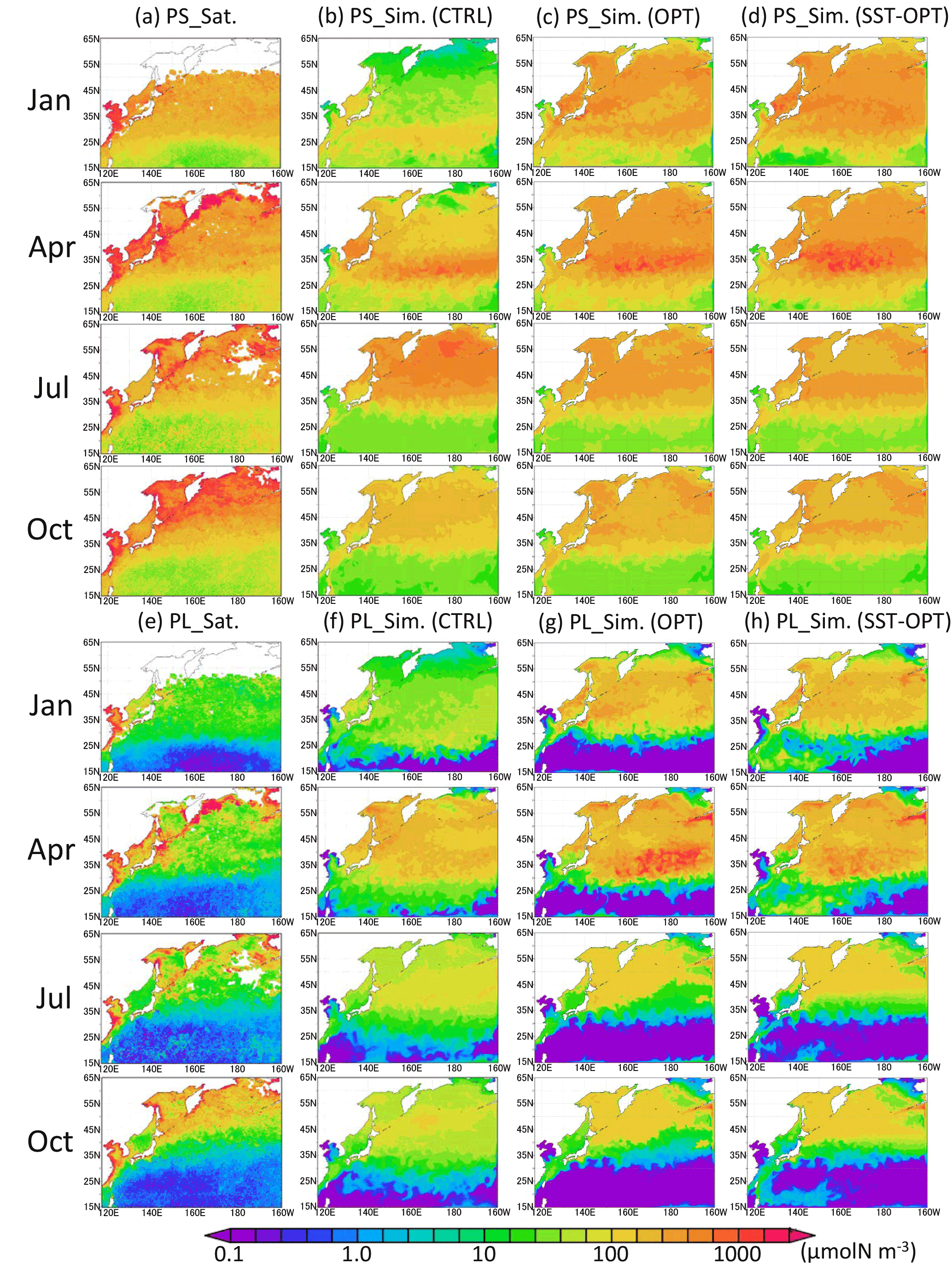
Figure 4Horizontal distribution of phytoplankton at the surface in 1998. (a) PS (small phytoplankton) from satellite observations, (b) PS in the control case, (c) PS in the parameter-optimized case, and (d) PS in the SST-dependent case. Panels (e)–(h) are the same except for PL (large phytoplankton). Areas without satellite data are left blank.
Lagged (within ± 2 months) correlation coefficients were calculated for the monthly time series of the surface phytoplankton concentration between the simulations and satellite data in each grid (Fig. 5a, c, e). Although there are some regions where the correlation values are out of the range in the 95 % significance level (Fig. 5b, d, f) due to the small numbers of monthly mean data, the correlation maps of CTRL, OPT, and SST-OPT can be relatively comparable to each other because of the same sample numbers of the simulations in each grid. Spatial distributions of the correlation show that the larger coefficient-value region (r > 0.7) of the OPT (Fig. 5c) in 25–45∘ N becomes more extended than that of the CTRL (Fig. 5a) by 71 %, though the mean value of the OPT in the north part of 50∘ N (r=0.18) is smaller than that in the CTRL (r=0.66). The result is similar in the SST-OPT (Fig. 5e). Our parameter estimation significantly improves the simulation result of the horizontal distribution of phytoplankton in the lower latitude (< 45∘ N), but not in the region (> 50∘ N) closer to the coasts.
Figure 6a–c show vertical distributions of total phytoplankton along the 165∘ E transect. The parameter optimization improves the distributions in that the phytoplankton maximum in the subsurface deepens more than that of CTRL (Fig. 6b, c). Parameter-optimized total biomass through the vertical section above 200 m is also closer to the observed data than the CTRL. It is an interesting result because the vertical distribution is improved due to the data-assimilation process using only surface satellite data. The detailed reason is discussed in Sect. 3.4. In the nutrient distribution along the 165∘ E (Fig. 6d to i), the concentrations of OPT (Fig. 6f, i) are lower than those of CTRL (Fig. 6e, h). The mean values along the transect of nitrate and silicate are 0.011 mol N m−3 and 0.025 mol Si m−3, respectively, in the OPT, 0.014 mol N m−3 and 0.034 mol Si m−3 in the CTRL, and 0.012 mol N m−3 and 0.022 mol Si m−3 in the observation (Fig. 6d, g). OPT is more consistent than CTRL with the observation, though the nitrate observed value is higher than the simulations in the surface (< 80 m) and subarctic (> 42∘ N) regions. While nitrate is not the limiting nutrient compared with iron and silicate for phytoplankton's photosynthesis in the subarctic region (this detail is also mentioned in Sect. 3.4), the data-assimilation process improves even the nutrient field in addition to the phytoplankton field.
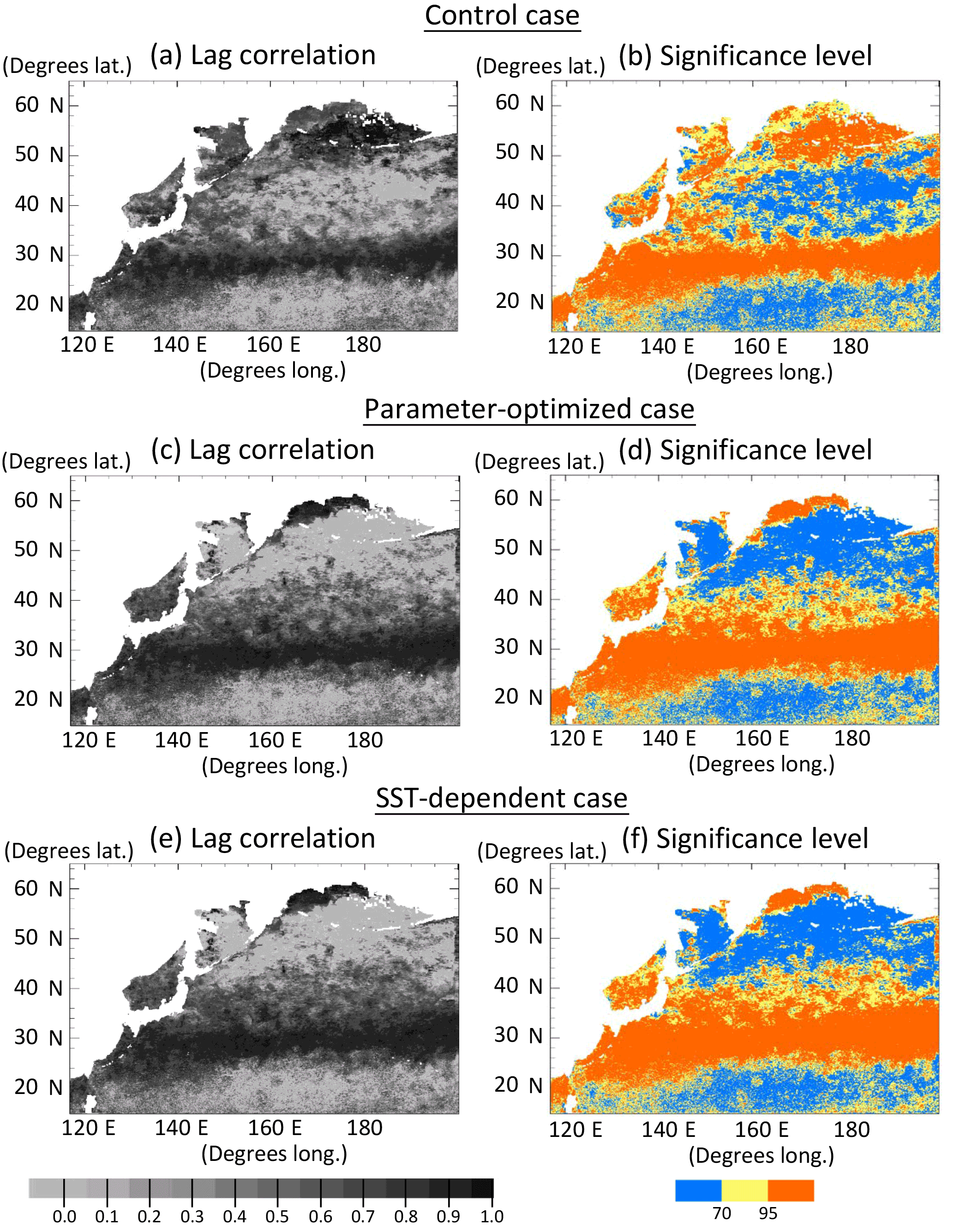
Figure 5Horizontal distribution of lagged (within ±2 months) correlation coefficients for the monthly time series of phytoplankton (PL + PS) concentration between the simulation and the satellite data in each grid at the surface in 1998, and the significance levels. (a, b) Control case, (c, d) parameter-optimized case, and (e, f) SST-dependent case. Areas with less than the number of seven monthly mean satellite data and in the coastal regions where the bottoms are less than 200 m are left blank.
As for the temperature and salinity along the vertical section (Fig. 7), the physical field used by the model simulations is well reconstructed in terms of mixed-layer depth and transition from the subarctic and the subtropical regions. Judging from the temperature and salinity distributions in the subarctic region (> 42∘ N), the water columns are well mixed vertically in both the observation and the simulation and intensely stratified in the subtropical region (< 36∘ N). There is the transition region (36–40∘ N) of temperature between the subtropical and the subarctic.
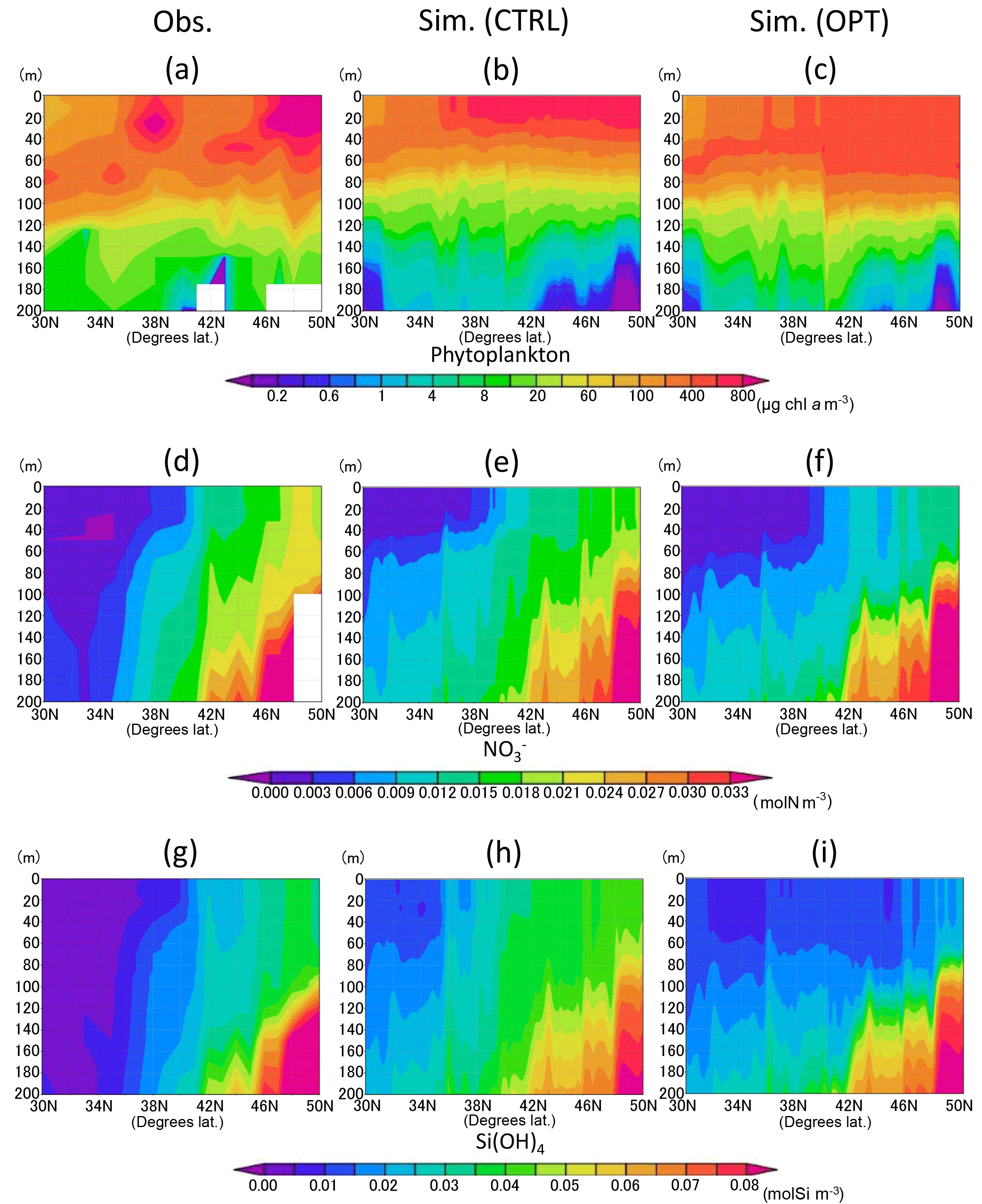
Figure 6Vertical distribution of phytoplankton (a–c), nitrate (d–f), and silicate (g–i) along the 165∘ E section in June 1998. (a, d, g) Data in situ observed during 16 to 21 June 1998 downloaded from the World Ocean Database 2013. (b, e, h) Simulation result of the control case mean in June 1998. (c, f, i) Simulation result of the parameter-optimized case mean in June 1998. Areas of missing values are left blank.
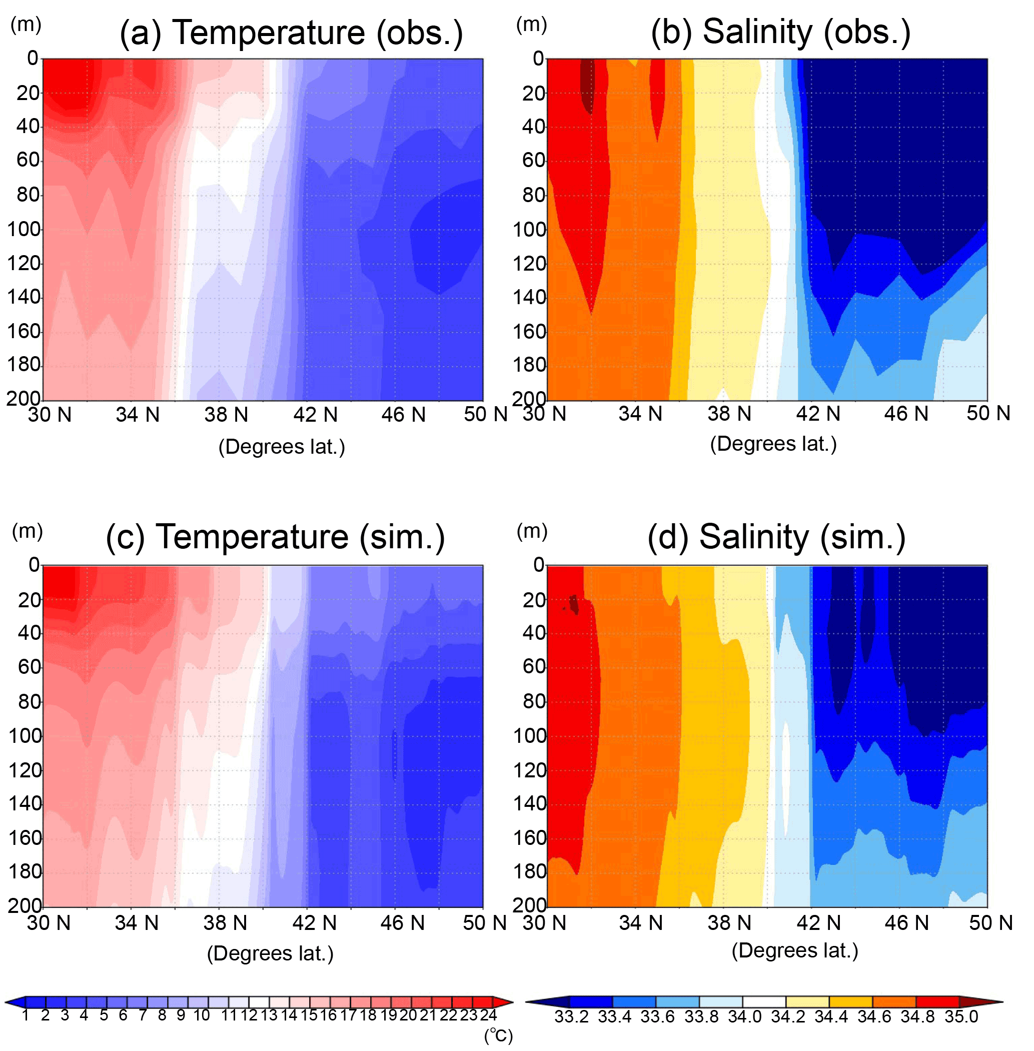
Figure 7Vertical distribution of temperature (a, c) and salinity (b, d) along the 165∘ E section in June 1998. (a, b) Data in situ observed during 16 to 21 June in 1998 downloaded from World Ocean Database 2013. (c, d) Physical field in June 1998 mean used in the 3-D NSI-MEM.
3.3 Amplitude and phase of seasonal variation in phytoplankton
The model performances were significantly improved in terms of spatial distributions of phytoplankton biomass, as a result of the parameters optimized in Sect. 3.2. Also at the specific stations of KNOT and S1, where the parameters were estimated using the 1-D simulations, seasonal variations in total phytoplankton concentrations in the OPT are generally better reproduced to those in the satellite data than those in the CTRL (Fig. 8). At KNOT (Fig. 8a), the phytoplankton bloom in the OPT occurs in winter, and the phytoplankton bloom in the CTRL occurs in summer in an anti-phase to that of the satellite. At S1 (Fig. 8b), the OPT case reasonably captures the timing of the phytoplankton bloom by the satellite, although the amplitude is slightly overestimated. The seasonal variations in the PS and PL concentrations are similar to those of the total phytoplankton (not shown) in both cases.
Figure 9 shows comparisons of the amplitude and the phase of seasonal variations between three model cases (CTRL, OPT, and SST-OPT) and the satellite data. The radius shows the amplitude of seasonal variation for each of the modelled cases relative to the satellite data, and the angle from the x axis shows the maximum concentration time lag for each of the model cases (i.e. the point (1, 0) shown as “true” is a match within 1 month and 30∘ error range to the satellite data). At KNOT, the OPT (blue solid vector) exhibits the phase closest to the satellite data among the three modelled cases. The ratios of the amplitudes to the satellite data are as follows: 1.00 for the OPT (blue solid vector), 1.08 for the SST-OPT (yellow solid vector), and 1.24 for the CTRL (orange solid vector). The timings of the maximum concentration are as follows: a 2-month delay for the OPT, a 3-month delay for the SST-OPT, and a 6-month delay (anti-phase) for the CTRL. The timing of the OPT at S1 (blue dotted vector) is improved, though its seasonal amplitude is not.
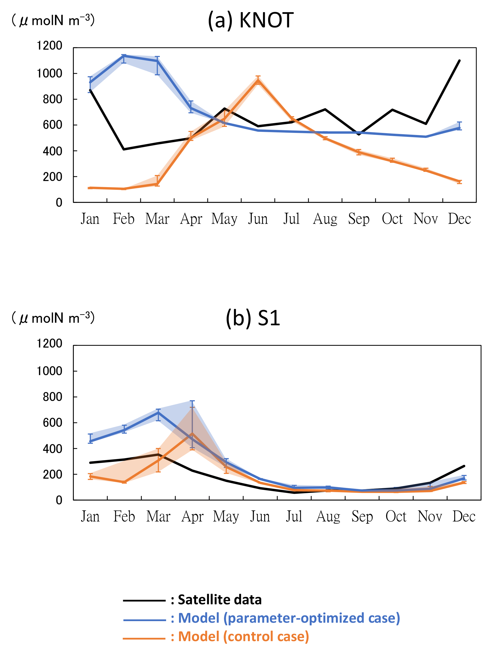
Figure 8Time series of phytoplankton (PL + PS) concentration in the 3-D NSI-MEM and satellite data at (a) KNOT and (b) S1. Error bars and shade of the simulations show the maximum and minimum values in ±0.3∘ around the grids of KNOT and S1.
Optimization of the physiological parameters by assimilating the satellite data at the two stations improves the seasonal variations in the phytoplankton concentrations such as the timing of the maximum concentration and the seasonal amplitude of the WNP region.
3.4 Vertical distributions of phytoplankton and nutrient concentrations at KNOT
The model-simulated vertical distributions of phytoplankton, nitrate, and silicate concentrations at KNOT on 20 July 1998 were compared with the observed ones on the same day (Fig. 10). The vertical distribution of phytoplankton (Fig. 10a) from 3-D simulations in the OPT (solid blue line) is closer to the in situ data (black line) compared to the CTRL (solid orange line): the maximum phytoplankton concentration for the OPT and the in situ data is located in the subsurface around a depth of 50 m, while there is no subsurface maximum in the CTRL. The differences in the biomass between the OPT and CTRL become especially larger in the subsurface layer (40 to 80 m). Thus, better physiological parameterization through the data assimilation improves not only the surface concentration but also the important characteristics of vertical plankton distribution such as the subsurface maximum. This is an interesting improvement because the physiological parameters are optimized using only surface satellite data.
The vertical profile of phytoplankton obtained from the 3-D simulation reproduces the observed ones better than the 1-D simulation, too (Fig. 10a). In addition, the difference in 3-D (solid lines) and 1-D (dashed lines) is larger in the upper layer (< 80 m) than in the lower layer (> 100 m). Moreover, error bars and shade for the 3-D simulations, which depict the maximum and minimum values in ±0.3∘ around the exact grid of KNOT, are also larger in the upper layer than the lower layer. We assume that horizontal advection such as mesoscale eddies is in the O (100 km) radius scale and ⩾ 16 weeks of lifetime (e.g. Chelton et al., 2011) and can be detected within the ±0.3∘ range in the physical field. These suggest that effects of horizontal advection are important for the daily reconstruction of the profile in the upper layer as the effects are not included in the 1-D model.
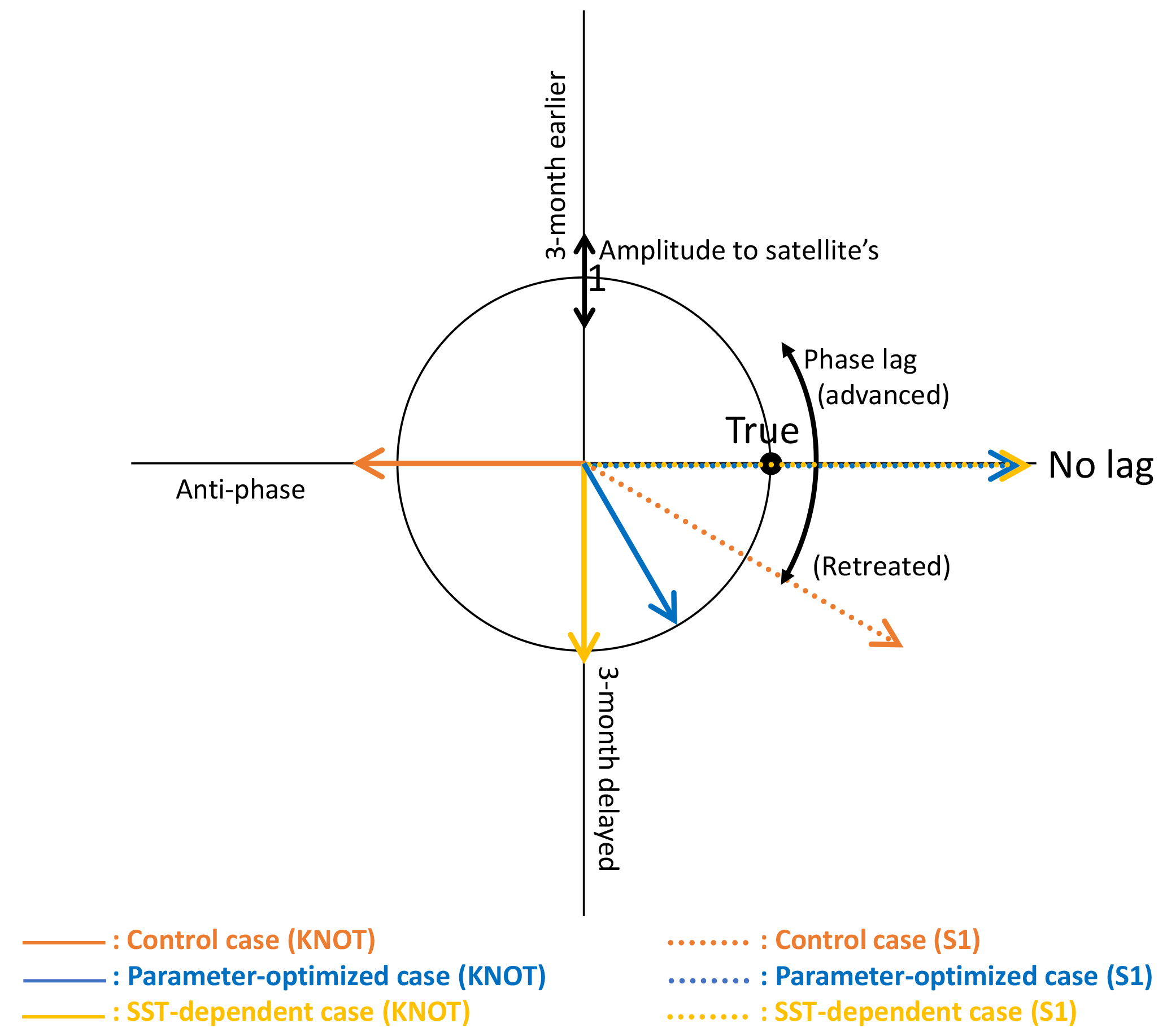
Figure 9Diagram showing the amplitude and the phase of seasonal variations in the three model cases compared with those in the satellite data. Based on the seasonal variation in the satellite data, the radius indicates the relative amplitude (model/satellite) of seasonal variation for each model case and the angle from the positive x axis shows the time lag of the maximum concentration for each model case (i.e. the point (1, 0) shown as “true” is a match within 1 month and a 30∘ error range to the satellite data). The blue dotted line (parameter-optimized case at S1) and yellow dotted line (SST-dependent case at S1) overlap on the no-lagged x axis.
In the NEMURO, the predecessor version of the NSI-MEM, the amplitude and timing of phytoplankton blooms are predominantly controlled by the photosynthesis rate (i.e. bottom-up effect of nutrient dependence) rather than the grazing rate (i.e. top-down effect of zooplankton) (Hashioka et al., 2013). The former is determined by the limited growth rate, which is a limitation function of growth rate by nitrogen (NH4 + NO3), silicate (Si(OH)4), or dissolved iron (FeD) (refer to Eqs. (A15) and (A23) in Shigemitsu et al., 2012). The smallest limited growth rate among the three nutrient groups (i.e. NH4 + NO3, Si(OH)4, and FeD) is used to limit the rate of phytoplankton's photosynthesis. For PS and PL in the OPT and CTRL, the dissolved-iron-limited growth rates (red lines in Fig. 11) dominate the photosynthesis, while the silicate growth rate is the second-largest limiting factor for PL (green lines in Fig. 11b). The mean iron-growth rates increase remarkably below a depth of 50 m (e.g. 0.37 to 1.86 and 0.48 to 2.47 day−1 in PS and PL, respectively) because of the parameter optimization of the potential maximum growth rate (V0) and the affinity (A0) as shown in Table 2. As a result, the uptake of dissolved iron seems to be accelerated, particularly in the subsurface layer, leading to an increase in the phytoplankton biomass (Fig. 10a). The larger biomass of phytoplankton may also consume more nitrate and silicate nutrients, resulting in lower nitrate (Fig. 10b) and silicate (Fig. 10c) concentrations above a depth of 140 m compared to that in the CTRL. The vertical gradients of nitrate and silicate in the OPT are closer to the observed data than those in the CTRL. In the OPT, nitrate and silicate concentrations are less than the data in situ, at the depth of both around 50 m (0.010 mol N m−3 and 0.015 mol Si m−3 in the OPT; 0.015 mol N m−3 and 0.025 mol Si m−3 in the observation) and 200 m (0.031 mol N m−3 and 0.069 mol Si m−3; 0.038 mol N m−3 and 0.085 mol Si m−3, respectively), while those at the depth of around 50 m in the CTRL (0.017 mol N m−3 and 0.037 mol Si m−3) are higher than those in the observed data, in which smaller vertical gradients of CTRL than the OPT are found. In the upper layer, the nutrients are adequately supplied to phytoplankton as a result of the parameter optimization. As in the lower layer below the depth of 120 m, the nutrient concentrations seem to also be determined by physical processes at the ocean-basin scale, not only local biological processes.
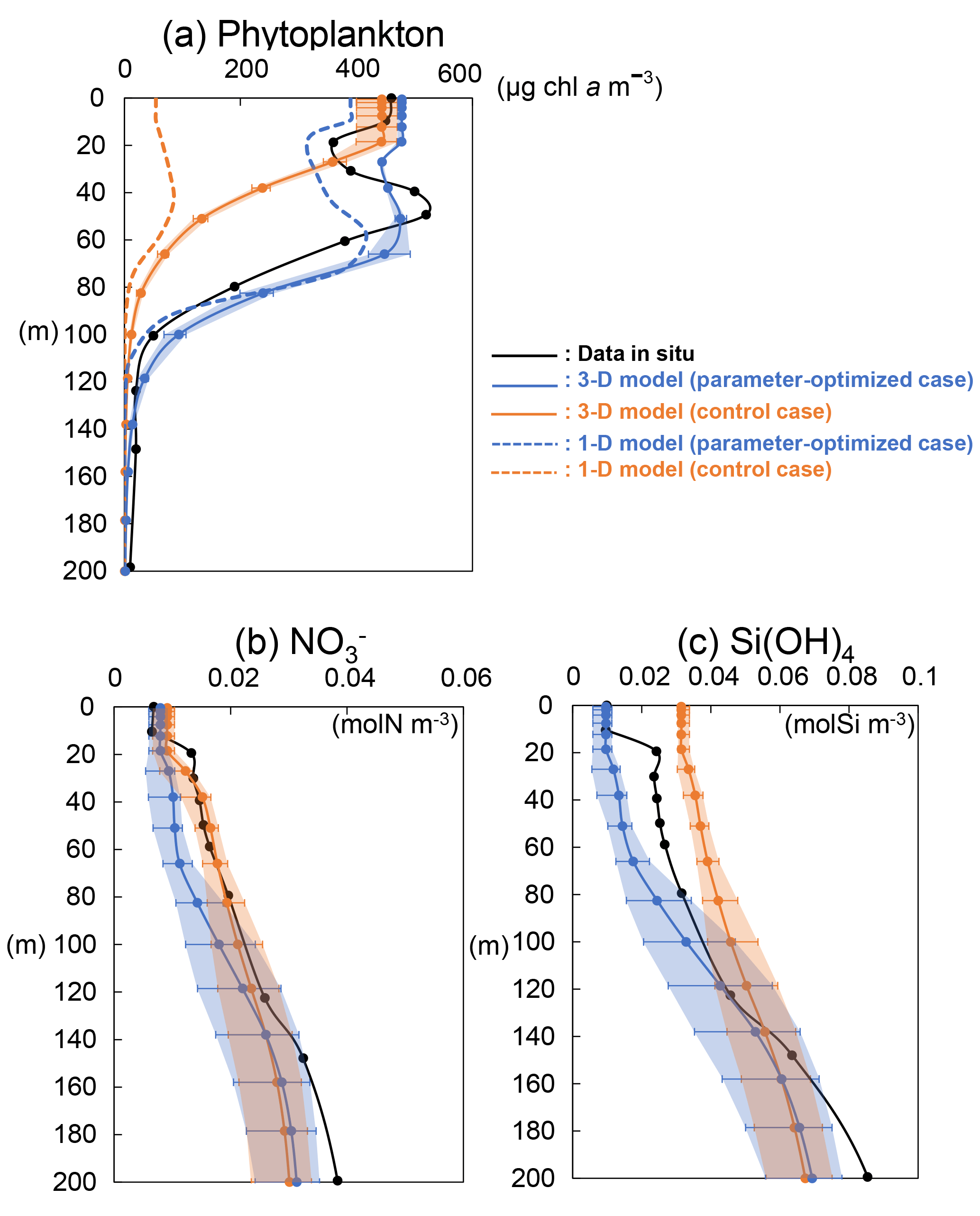
Figure 10Vertical distributions of (a) phytoplankton (PL + PS) from the 3-D model (solid line), 1-D model (dashed line), and in situ data; (b) nitrate and (c) silicate concentrations from the 3-D model (solid line) and in situ data at KNOT on 20 July 1998. Error bars and shade of the 3-D simulations show the same mean as those of Fig. 8.
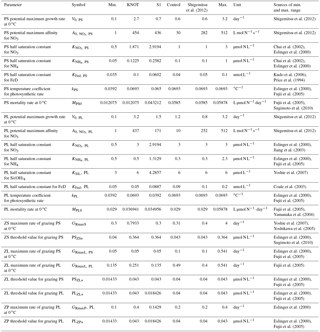
Table 2NSI-MEM physiological parameters estimated by the μ-GA. Maximum and minimum values prescribe the upper and lower bounds of the parameter variations used in the previous studies. KNOT and S1 indicate optimal estimated values in the provinces of Fig. 1b while control values are not optimized parameter values, and the values of Shigemitsu et al. (2012) are the parameters of the previous study.
The change of the dissolved-iron-limited growth rates by optimization results in the lower concentration of dissolved iron in the subarctic area (Fig. 12) because of the greater consumption of FeD by the phytoplankton than in the CTRL. The result is so far consistent with the conception of an HNLC region in the North Pacific Ocean (Moore et al., 2013), in spite of the fact that our model does not include the Sea of Okhotsk as another iron source to the WNP region (Nishioka et al., 2011). A further improvement is expected by adding such an iron supply into our model.
3.5 Physiological parameter changes with ambient conditions
The SST-OPT (i.e. smoothed changing parameters) was compared to the OPT (i.e. boundary-gap parameters). The horizontal distribution of the PS and PL concentrations in the SST-OPT are not significantly different from those in the OPT (Fig. 4) except in two regions – the western region of low latitude (15 to 25∘ N and 120 to 150∘ E during January and April in Fig. 4h), and the region adjacent to the Kuroshio Extension (around 40∘ N during July to October in Fig. 4h). The former exception is due to the extrapolation of parameters with high SST and the latter is due to smoothing of parameters between the KNOT and S1 stations. The simulated seasonal variations in phytoplankton concentration in the SST-OPT are slightly worse than those in the OPT at the two stations (Fig. 9). The ratios of the seasonal amplitudes at S1, for instance, were 2.33 for the OPT and 2.39 for the SST-OPT. The maximum concentrations for both cases are found in the same month (March) as that for the satellite data (they overlap each other on the no-lagged x axis in Fig. 9). However, a smoothed set of parameters dependent on the SST prevents the artificial gap of the parameter value at the fixed boundary between the two provinces.
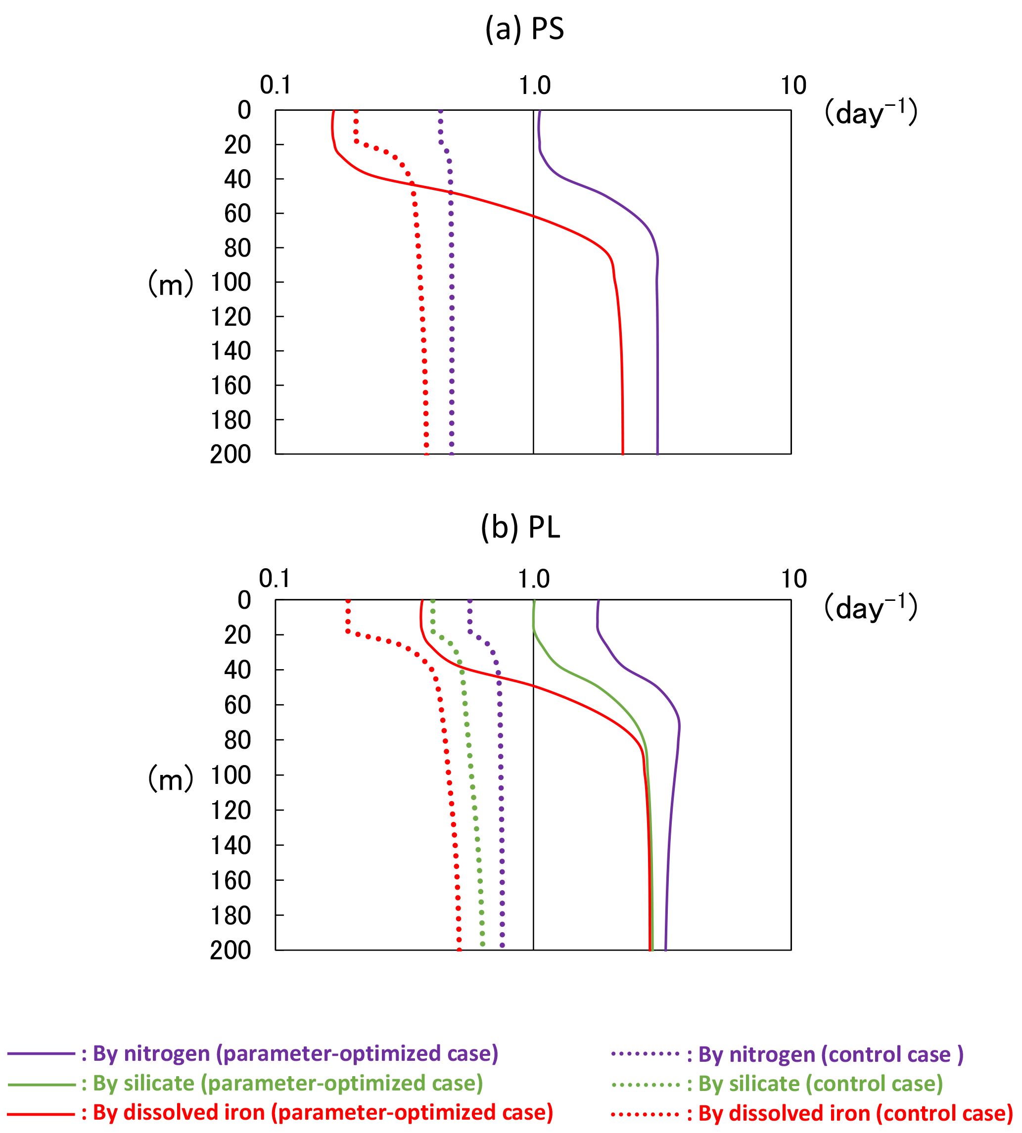
Figure 11Vertical distributions of limited growth rates by nitrogen, silicate, and dissolved iron simulated from the 3-D model of (a) PS and (b) PL at KNOT on 20 July 1998. The smallest rate of dissolved iron most heavily limits the rate of phytoplankton's photosynthesis. These limited growth rates (mol N m−3 day−1) were divided by the PS or PL biomass (mol N m−3) to standardize.
Physiological parameters represented in ecosystem models were optimized in reference to 1998 while they may change with time. In addition, they may change with the surrounding conditions in the real ocean (e.g. SST, nutrient abundance, and light intensity). Smith and Yamanaka (2007) and Smith et al. (2009) suggest the significance of photo-acclimation and nutrient affinity acclimation. Phytoplankton cells change their traits (e.g. nutrient channel, enzyme) in response to ambient nutrient concentrations, and typically large (small) cells adapt to low (high) light and high (low) nutrient concentrations (Smith et al., 2015). In the NSI-MEM, the effect of nutrient-uptake responses by plankton acclimated to different ambient nutrient conditions is applied as an OU kinetic formulation, but the effect of photo-acclimation has not yet been introduced. Incorporation of temporal variation in the physiological parameters may be effective in precisely reproducing distributions and variations in phytoplankton. In other words, data assimilation through the physiological parameter change with environmental conditions might play the part in a calibration of simplified formulations of LTL marine ecosystem models. However, four-dimensional changes of physiological parameters complicate scientific interpretation (Schartau et al., 2017), even though marine ecosystem models have been developed in order to simplify real-world marine ecosystems and facilitate scientific interpretation. The spatial parameter estimation was conducted in this study because we would like to also discuss the physiological effects of parameters changing in detail.
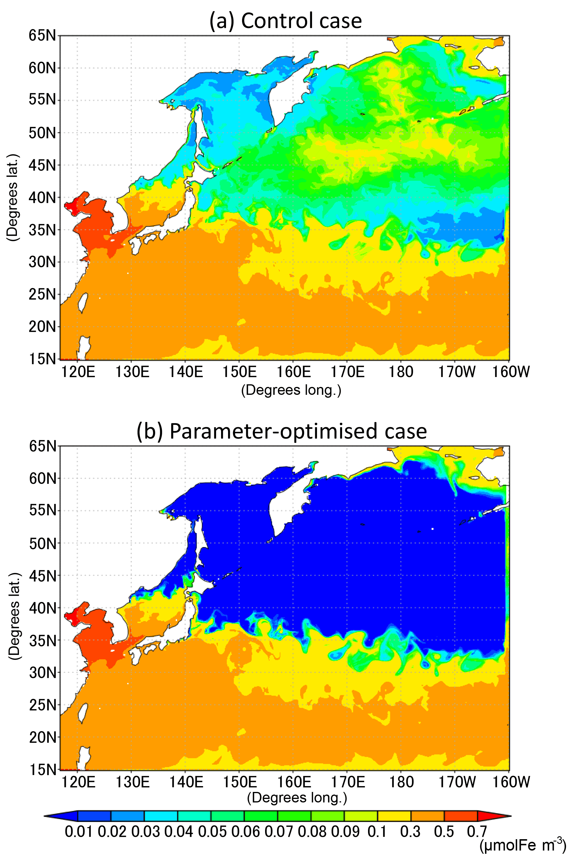
Figure 12Horizontal distribution of dissolved iron in the surface seawater layer for July 1998; (a) control case and (b) parameter-optimized case.
We extended an LTL marine ecosystem model, NSI-MEM, into a 3-D coupled OGCM. We also used a data assimilation approach for two different PFTs in the WNP region: non-diatom PS and PL. In the NSI-MEM, 23 ecosystem parameters were estimated using a 1-D emulator with a μ-GA parameter-optimization procedure. By applying the optimized parameters to the 3-D NSI-MEM, the model performances were improved in terms of the seasonal variations in phytoplankton biomass, including the timing of the plankton bloom in the surface layer, compared to those using prior parameter values (control case). Notably, the vertical distribution of phytoplankton such as the subsurface maximum layer was also improved via the parameter optimization, compared to that in the control case. Thus, it was demonstrated that the 3-D simulation performed better than the 1-D simulation even to reproduce the vertical profile of phytoplankton.
Physiological parameters in this study were systematically determined by a μ-GA within the range of those used by numerical models in previous studies. While our parameter estimation improved the modelling skill of temporal and spatial variability in PL and PS in the WNP, the estimated parameter values themselves should also be confirmed with a sufficient number of data when they become available, in order to increase our confidence towards mechanistic and numerical understanding of the phytoplankton dynamics observed.
The phytoplankton satellite data were downloaded from the Ocean Colour Climate Change Initiative, ESA (European Space Agency), available online at http://www.esa-oceancolour-cci.org/ (last access: 28 May 2018) (free access). The SST satellite data were downloaded from the National Oceanic and Atmospheric Administration Pathfinder project in GHRSST (The Group for High Resolution Sea Surface Temperature) and the US National Oceanographic Data Center, available online at http://www.nodc.noaa.gov/SatelliteData/pathfinder4km/ (last access: 28 May 2018) (free access). The in situ data along the 165∘ E section were provided by the World Ocean Database 2013 https://www.nodc.noaa.gov/OC5/WOD13 (last access: 28 May 2018) (free access). The in situ data at KNOT are available for the only members of the Core Research for Evolutional Science and Technology (CREST) program. The files necessary to reproduce the simulations are available from the authors upon request.
The authors declare that they have no conflict of interest.
This study was supported by Core Research for Evolutional Science and
Technology (CREST), Japan Science and Technology Agency, grant number
JPMJCR11A5. The first author developed the 3-D NSI-MEM and conducted
simulations using this model at Hokkaido University and analysed the results
supported by the Center for Earth Surface System Dynamics, Atmosphere and
Ocean Research Institute, The University of Tokyo. The phytoplankton
satellite data were gathered by the Ocean Colour Climate Change Initiative,
ESA (European Space Agency). The SST satellite data were provided by the
National Oceanic and Atmospheric Administration Pathfinder project in GHRSST
(The Group for High Resolution Sea Surface Temperature) and the US National
Oceanographic Data Center. Data in situ used in this study were taken from
World Ocean Database 2013 and Ocean Time-Series program in the western North
Pacific.
Edited by: Eric J. M. Delhez
Reviewed by: two anonymous referees
Aumont, O. and Bopp, L.: Globalizing results from ocean in situ iron fertilization studies, Global Biogeochem. Cy., 20, GB2017, https://doi.org/10.1029/2005GB002591, 2006.
Blauw, A. N., Los, H. F. J., Bokhorst, M., and Erftemeijer, P. L. A.: GEM: a generic ecological model for estuaries and coastal waters, Hydrobiologia, 618, 175–198, 2009.
Buitenhuis, E. T., Rivkin, R. B., Sailley, S., and Le Quéré, C.: Biogeochemical fluxes through microzooplankton, Global Biogeochem. Cy., 24, GB4015, https://doi.org/10.1029/2009GB003601, 2010.
Chai, F., Dugdale, R., Peng, T., Wilkerson, F., and Barber, R.: One-dimensional ecosystem model of the equatorial Pacific upwelling system, Part I: model development and silicon and nitrogen cycle, Deep-Sea Res. Pt. II, 49, 2713–2745, 2002.
Chelton, D. B., Schlax, M. G., and Samelson, R. M.: Global observations of nonlinear mesoscale eddies, Prog. Oceanogr., 91, 167–216, 2011.
Coale, K. H., Wang, X., Tanner, S. J., and Johnson, K. S.: Phytoplankton growth and biological response to iron and zinc addition in the Ross Sea and Antarctic Circumpolar Current along 170 W, Deep-Sea Res. Pt II, 50, 635–653, 2003.
Cotrim da Cunha, L., Buitenhuis, E. T., Le Quéré, C., Giraud, X., and Ludwig, W.: Potential impact of changes in river nutrient supply on global ocean biogeochemistry, Global Biogeochem. Cy., 21, GB4007, https://doi.org/10.1029/2006GB002718, 2007.
Edwards, A. M. and Brindley, J.: Oscillatory behaviour in a three-component plankton population model, Dynam. Stabil. Syst., 11, 347–370, 1996.
Eslinger, D. L., Kashiwai, M. B., Kishi, M. J., Megrey, B. A., Ware, D. M., and Werner, F. E.: Final report of the international workshop to develop a prototype lower trophic level ecosystem model for comparison of different marine ecosystems in the north Pacific, PICES Scientific Report, 15, 1–77, 2000.
Fasham, M., Ducklow, H., and McKelvie, S.: A nitrogen-based model of plankton dynamics in the oceanic mixed layer, J. Mar. Res., 48, 591–639, 1990.
Fiechter, J., Herbei, R., Leeds, W., Brown, J., Milliff, R., Wikle, C., Moore, A., and Powell, T.: A Bayesian parameter estimation method applied to a marine ecosystem model for the coastal Gulf of Alaska, Ecol. Model., 258, 122–133, 2013.
Follows, M. J., Dutkiewicz, S., Grant, S., and Chisholm, S. W.: Emergent biogeography of microbial communities in a model ocean, Science, 315, 1843–1846, 2007.
Fujii, M., Yoshie, N., Yamanaka, Y., and Chai, F.: Simulated biogeochemical responses to iron enrichments in three high nutrient, low chlorophyll (HNLC) regions, Prog. Oceanogr., 64, 307–324, 2005.
Fujii, Y. and Kamachi, M.: Three-dimensional analysis of temperature and salinity in the equatorial Pacific using a variational method with vertical coupled temperature-salinity empirical orthogonal function modes, J. Geophys. Res.-Oceans, 108, 3297, https://doi.org/10.1029/2002JC001745, 2003.
Gregg, W. W. and Casey, N. W.: Global and regional evaluation of the SeaWiFS chlorophyll data set, Remote Sens. Environ., 93, 463–479, 2004.
Hashioka, T., Hirata, T., Chiba S., Noguchi-Aita, M., Nakano, H., and Yamanaka, Y.: Biogeochemical classification of the global ocean based on nutrient limitation of phytoplankton growth, Biogeosciences, in preparation, 2018.
Hashioka, T., Vogt, M., Yamanaka, Y., Le Quéré, C., Buitenhuis, E. T., Aita, M. N., Alvain, S., Bopp, L., Hirata, T., Lima, I., Sailley, S., and Doney, S. C.: Phytoplankton competition during the spring bloom in four plankton functional type models, Biogeosciences, 10, 6833–6850, https://doi.org/10.5194/bg-10-6833-2013, 2013.
Hirata, T., Hardman-Mountford, N. J., Brewin, R. J. W., Aiken, J., Barlow, R., Suzuki, K., Isada, T., Howell, E., Hashioka, T., Noguchi-Aita, M., and Yamanaka, Y.: Synoptic relationships between surface Chlorophyll-a and diagnostic pigments specific to phytoplankton functional types, Biogeosciences, 8, 311–327, https://doi.org/10.5194/bg-8-311-2011, 2011.
Hoshiba, Y. and Yamanaka, Y.: Simulation of the effects of bottom topography on net primary production induced by riverine input, Cont. Shelf Res., 117, 20–29, 2016.
Itoh, S., Yasuda, I., Saito, H., Tsuda, A., and Komatsu, K.: Mixed layer depth and chlorophyll a: Profiling float observations in the Kuroshio-Oyashio Extension region, J. Marine Syst., 151, 1–14, 2015.
Jiang, M., Chai, F., Dugdale, R., Wilkerson, F., Peng, T., and Barber, R.: A nitrate and silicate budget in the equatorial Pacific Ocean: a coupled physical-biological model study, Deep-Sea Res. Pt. II, 50, 2971–2996, 2003.
Jickells, T. D.: Nutrient biogeochemistry of the coastal zone, Science, 281, 217–221, 1998.
Kishi, M. J., Kashiwai, M., Ware, D. M., Megrey, B. A., Eslinger, D. L., Werner, F. E., Noguchi-Aita, M., Azumaya, T., Fujii, M., and Hashimoto, S.: NEMURO – a lower trophic level model for the North Pacific marine ecosystem, Ecol. Model., 202, 12–25, 2007.
Krishnakumar, K.: Micro-genetic algorithms for stationary and non-stationary function optimization, Proc. SPIE, 1196, https://doi.org/10.1117/12.969927, 1990.
Kudo, I., Noiri, Y., Nishioka, J., Taira, Y., Kiyosawa, H., and Tsuda, A.: Phytoplankton community response to Fe and temperature gradients in the NE (SERIES) and NW (SEEDS) subarctic Pacific Ocean, Deep-Sea Res. Pt. II, 53, 2201–2213, 2006.
Kuroda, H. and Kishi, M. J.: A data assimilation technique applied to estimate parameters for the NEMURO marine ecosystem model, Ecol. Model., 172, 69–85, 2004.
Lancelot, C., Hannon, E., Becquevort, S., Veth, C., and De Baar, H. J. W.: Modeling phytoplankton blooms and carbon export production in the Southern Ocean: dominant controls by light and iron in the Atlantic sector in Austral spring 1992, Deep-Sea Res. Pt. I, 47, 1621–1662, 2000.
Large, W. G. and Yeager, S. G.: The global climatology of an interannually varying air-sea flux data set, Clim. Dynam., 33, 341–364, 2009.
Longhurst, A.: Seasonal cycles of pelagic production and consumption, Prog. Oceanogr., 36, 77–167, 1995.
Michaelis, L., Menten, M. L., Johnson, K. A., and Goody, R. S.: The original Michaelis constant: translation of the 1913 Michaelis-Menten paper, Biochemistry, 50, 8264–8269, 2011.
Moore, C. M., Mills, M. M., Arrigo, K. R., Berman-Frank, I., Bopp, L., Boyd, P. W., Galbraith, E. D., Geider, R. J., Guieu, C., Jaccard, S. L., Jickells, T. D., La Roche, J., Lenton, T. M., Mahowald, N. M., Marañón, E., Marinov, I., Moore, J. K., Nakatsuka, T., Oschlies, A., Saito, M. A., Thingstad, T. F., Tsuda, A., and Ulloa, O.: Processes and patterns of oceanic nutrient limitation, Nat. Geosci., 6, 701–710, 2013.
Nishioka, J., Ono, T., Saito, H., Sakaoka, K., and Yoshimura, T.: Oceanic iron supply mechanisms which support the spring diatom bloom in the Oyashio region, western subarctic Pacific, J. Geophys. Res.-Oceans, 116, C02021, https://doi.org/10.1029/2010JC006321, 2011.
Parekh, P., Follows, M., and Boyle, E.: Modeling the global ocean iron cycle, Global Biogeochem. Cy., 18, GB1002, https://doi.org/10.1029/2003GB002061, 2004.
Price, N., Ahner, B., and Morel, F.: The equatorial Pacific Ocean: Grazercontrolled phytoplankton populations in an iron-limited ecosystem, Limnol. Oceanogr., 39, 520–534, 1994.
Qiu, B. and Chen, S.: Eddy-mean flow interaction in the decadally modulating Kuroshio Extension system, Deep-Sea Res. Pt. II, 57, 1098–1110, 2010.
Schartau, M., Wallhead, P., Hemmings, J., Löptien, U., Kriest, I., Krishna, S., Ward, B. A., Slawig, T., and Oschlies, A.: Reviews and syntheses: parameter identification in marine planktonic ecosystem modelling, Biogeosciences, 14, 1647–1701, https://doi.org/10.5194/bg-14-1647-2017, 2017.
Shigemitsu, M., Okunishi, T., Nishioka, J., Sumata, H., Hashioka, T., Aita, M., Smith, S., Yoshie, N., Okada, N., and Yamanaka, Y.: Development of a onedimensional ecosystem model including the iron cycle applied to the Oyashio region, western subarctic Pacific, J. Geophys. Res.-Oceans, 117, C06021, https://doi.org/10.1029/2011JC007689, 2012.
Smith, S. L. and Yamanaka, Y.: Quantitative comparison of photoacclimation models for marine phytoplankton, Ecol. Model., 201, 547–552, 2007.
Smith, S. L., Yamanaka, Y., Pahlow, M., and Oschlies, A.: Optimal uptake kinetics: physiological acclimation explains the pattern of nitrate uptake by phytoplankton in the ocean, Mar. Ecol.-Prog. Ser., 384, 1–12, 2009.
Smith, S. L., Pahlow, M., Merico, A., Acevedo-Trejos, E., Sasai, Y., Yoshikawa, C., Sasaoka, K., Fujiki, T., Matsumoto, K., and Honda, M. C.: Flexible phytoplankton functional type (FlexPFT) model: size-scaling of traits and optimal growth, J. Plankton Res., 38, 977–992, 2015.
Sugimoto, R., Kasai, A., Miyajima, T., and Fujita, K.: Modeling phytoplankton production in Ise Bay, Japan: Use of nitrogen isotopes to identify dissolved inorganic nitrogen sources, Estuar. Coast. Shelf. S., 86, 450–466, 2010.
Sumata, H., Hashioka, T., Suzuki, T., Yoshie, N., Okunishi, T., Aita, M. N., Sakamoto, T. T., Ishida, A., Okada, N., and Yamanaka, Y.: Effect of eddy transport on the nutrient supply into the euphotic zone simulated in an eddy-permitting ocean ecosystem model, J. Mar. Syst., 83, 67–87, 2010.
Toyoda, T., Awaji, T., Masuda, S., Sugiura, N., Igarashi, H., Sasaki, Y., Hiyoshi, Y., Ishikawa, Y., Saitoh, S., and Yoon, S.: Improved state estimations of lower trophic ecosystems in the global ocean based on a Green's function approach, Prog. Oceanogr., 119, 90–107, 2013.
Tsuda, A., Takeda, S., Saito, H., Nishioka, J., Nojiri, Y., Kudo, I., Kiyosawa, H., Shiomoto, A., Imai, K., Ono, T., Shimamoto, A., Tsumune, D., Yoshimura, T., Aono, T., Hinuma, A., Kinugasa, M., Suzuki, K., Sohrin, Y., Noiri, Y., Tani, H., Deguchi, Y., Tsurushima, N., Ogawa, H., Fukami, K., Kuma, K., and Saino, T.: A mesoscale iron enrichment in the western subarctic Pacific induces a large centric diatom bloom, Science, 300, 958–961, 2003.
Tsujino, H., Hirabara, M., Nakano, H., Yasuda, T., Motoi, T., and Yamanaka, G.: Simulating present climate of the global ocean-ice system using the Meteorological Research Institute Community Ocean Model (MRI. COM): simulation characteristics and variability in the Pacific sector, J. Oceanogr., 67, 449–479, 2011.
Tsurushima, N., Nojiri, Y., Imai, K., and Watanabe, S.: Seasonal variations of carbon dioxide system and nutrients in the surface mixed layer at station KNOT (44 N, 155 E) in the subarctic western North Pacific, Deep-Sea Res. Pt. II, 49, 5377–5394, 2002.
Usui, N., Ishizaki, S., Fujii, Y., Tsujino, H., Yasuda, T., and Kamachi, M.: Meteorological Research Institute multivariate ocean variational estimation (MOVE) system: Some early results, Adv. Space Res., 37, 806–822, 2006.
Watanabe, S., Hajima, T., Sudo, K., Nagashima, T., Takemura, T., Okajima, H., Nozawa, T., Kawase, H., Abe, M., Yokohata, T., Ise, T., Sato, H., Kato, E., Takata, K., Emori, S., and Kawamiya, M.: MIROC-ESM 2010: model description and basic results of CMIP5-20c3m experiments, Geosci. Model Dev., 4, 845–872, https://doi.org/10.5194/gmd-4-845-2011, 2011.
Xiao, Y. and Friedrichs, M. A. M.: The assimilation of satellite-derived data into a one-dimensional lower trophic level marine ecosystem model, J. Geophys. Res.-Oceans, 119, 2691–2712, 2014.
Yamanaka, Y., Yoshie, N., Fujii, M., Aita, M. N., and Kishi, M. J.: An ecosystem model coupled with Nitrogen-Silicon-Carbon cycles applied to Station A7 in the Northwestern Pacific, J. Oceanogr., 60, 227–241, 2004.
Yoshie, N., Yamanaka, Y., Rose, K. A., Eslinger, D. L., Ware, D. M., and Kishi, M. J.: Parameter sensitivity study of the NEMURO lower trophic level marine ecosystem model, Ecol. Model., 202, 26–37, 2007.
Yoshikawa, C., Yamanaka, Y., and Nakatsuka, T.: An ecosystem model including nitrogen isotopes: perspectives on a study of the marine nitrogen cycle, J. Oceanogr., 61, 921–942, 2005.