Decorrelation scales for Arctic Ocean hydrography – Part I: Amerasian Basin

Any use of observational data for data assimilation requires adequate information of their representativeness in space and time. This is particularly important for sparse, non-synoptic data, which comprise the bulk of oceanic in situ observations in the Arctic. To quantify spatial and temporal scales of temperature and salinity variations, we estimate the autocorrelation function and associated decorrelation scales for the Amerasian Basin of the Arctic Ocean. For this purpose, we compile historical measurements from 1980 to 2015. Assuming spatial and temporal homogeneity of the decorrelation scale in the basin interior (abyssal plain area), we calculate autocorrelations as a function of spatial distance and temporal lag. The examination of the functional form of autocorrelation in each depth range reveals that the autocorrelation is well described by a Gaussian function in space and time. We derive decorrelation scales of 150–200 km in space and 100–300 days in time. These scales are directly applicable to quantify the representation error, which is essential for use of ocean in situ measurements in data assimilation. We also describe how the estimated autocorrelation function and decorrelation scale should be applied for cost function calculation in a data assimilation system.

1 Introduction

Any use of observational data requires assumptions, or better knowledge, about the representativeness of each measurement in space and time. This holds even more for in situ observations from data-sparse regions, such as the Arctic Ocean. Interpolation guided by the statistical properties of observed quantities can provide Arctic-wide fields, while data assimilation using comprehensive dynamical models and assimilation methods can, in addition, provide fields that are consistent with the modeled physics. Also, sampling strategies have to take the knowledge of the representativeness of point measurement into account. The temporal and spatial scales, for which a single measurement is representative, depend on local dynamics, external forcing, and the influence of lateral water–mass influxes. Here, we make an attempt to estimate those length scales and timescales in the Arctic Ocean based on observational data from the period 1980–2015. This will be achieved by estimating the autocorrelation function and decorrelation scales of temperature and salinity.

Autocorrelation functions and associated decorrelation scales are useful measures to characterize physical phenomena occurring in the ocean (Stammer, 1997; Eden, 2007). These functions describe spatial and temporal ranges over which ocean properties coherently vary, and the scales provide a measure of the spatial and temporal extent of the variations. The functional form of the autocorrelation depends on the physical properties, the considered scales (e.g., synoptic versus mesoscale) and the area. Many studies have estimated autocorrelation functions through analysis of in situ ocean measurements (e.g., Meyers et al., 1991; Chu et al., 2002; Delcroix et al., 2005) and satellite observations (e.g., Kuragano and Kamachi, 2000; Hosoda and Kawamura, 2004; Tzorti et al., 2016). Generally, the estimated autocorrelation functions have exponential or Gaussian form (Molinari and Festa, 2000). The decorrelation scales are usually given by the e-folding scale of the corresponding autocorrelation functions (see McLean, 2010 for a summary of different definitions).

Estimated decorrelation scales have been applied to a variety of ocean studies. In the context of dynamical studies, the decorrelation scale is used as a measure of the scale of prevailing phenomena and used to relate dynamical processes with the observed signals (e.g., Stammer, 1997; Ito et al., 2004; Kim and Kosro, 2013). In optimal interpolation and objective mapping, the decorrelation scale gives a measure of influential radius of a point measurement; the autocorrelation function, together with the associated decorrelation scale, provides the weight of a point measurement on mean field estimates (Meyers et al., 1991; Chu et al., 1997; Davis, 1998; Wong et al., 2003; Böhme and Send, 2005). For observation network design, decorrelation scales are one guide to estimate optimal sampling intervals in space and time (Sprintall and Meyers, 1991; White, 1995; Delcroix et al., 2005).

One of the prevalent and growing applications of decorrelation scales is data assimilation. Data assimilation synthesizes observed data and modeled physics based on statistical theories. This is an effective approach to fill the gap between observation and modeling studies (Wunsch, 2006; Blayo et al., 2015). Generally, data assimilation minimizes a model–data misfit with an assessment of errors; the autocorrelation function and the decorrelation scale are necessary for these error assessments (Carton et al., 2000; Forget and Wunsch, 2007). For a model–data misfit calculation, the difference of the spatial (and temporal) scales represented by a model and by the observations should be taken into account. Physical properties simulated in general circulation models (GCMs) represent mean values over each grid cell for a certain temporal period, whereas those from in situ measurements represent values at a localized point in space and in time. The error resulting from the difference of the scales represented by these two approaches is referred to as representation error (see van Leeuwen, 2015 for a summary). The autocorrelation function and the decorrelation scales provide a direct measure of the representation error. In ocean data assimilation, an assessment of the representation error is particularly important, since it is generally an order of magnitude larger than the measurement (instrument) error (Ingleby and Huddleston, 2007).

A necessity of decorrelation scale in ocean data assimilation also comes from the sparseness of ocean measurements. An autocorrelation function is necessary to constrain locations distant from a measurement. Li et al. (2003) pointed out that an assimilation of sparsely distributed data into an eddy-permitting model, without taking its influential radius into account, causes serious problems around the locations where the data are assimilated. Artificial eddies appear around the location of the data, since the density at the data location differs from densities at their surrounding grid points in the model. They also pointed out that the assimilated information disappears on the timescale determined by the model's local advection and diffusion. Note that this situation cannot be solved by applying advanced data assimilation techniques (e.g., 4DVar, EnKF), since the artificial eddies are dynamically consistent with the modeled physics. Autocorrelation function and decorrelation scale provide necessary information to solve such problems by imposing a spatial and temporal radius of influence of each measurement (Forget and Wunsch, 2007; Zuo et al., 2011).

Practically, autocorrelation functions are used to define an “observation operator” in data assimilation systems. The observation operator maps modeled variables onto observational points. If the operator is properly defined, a point measurement will constrain the model, not only at the location where measurements exist but also in areas distant from the measurement. An implementation of such an observation operator makes it possible to fully exploit the potential of sparsely distributed measurements, and can solve problems such as those reported by Li et al. (2003). This is of particular importance as the ocean models used for assimilation become eddy-permitting. An additional important feature of the autocorrelation function is to constrain the scale of temporally varying fluctuations. Unlike the static interpolation approaches, data assimilation provides a four-dimensional analysis field. In order to appropriately assimilate observed temporal fluctuations, the temporal scale of fluctuations should be implemented in the observation operator.

In the midlatitude and equatorial regions, there are a number of decorrelation scale estimates (e.g., White and Meyers, 1982; Chu et al., 1997, 2002; Deser et al., 2003; Martins et al., 2015), and these have been applied for a variety of studies including data assimilation (see the papers mentioned above). On the other hand, while a few studies have examined scales of temperature and salinity variability in the Arctic Ocean (e.g., Timmermans and Winsor, 2013; Marcinko et al., 2015), there has been no assessment of basin-wide decorrelation scales of T∕S field to date. One reason is that sea-ice cover greatly inhibits sea surface observation by remote sensing. Another reason is the sparse coverage of in situ ocean measurements due to the inaccessibility and the absence of an Argo float network (that has provided essential data for midlatitude and Southern Ocean studies; e.g., McLean, 2010; Reeve et al., 2016). In the last decade, however, the number of observational activities has been increasing significantly, with the growing concern about the sea-ice retreat and its potential impact on global climate (see, e.g., Ortiz et al., 2011 and references therein). In addition to the increasing number of research cruises, autonomous observation platforms (e.g., ice-tethered profilers – ITPs; Krishfield et al., 2008a; Toole et al., 2011) now provide data throughout a full seasonal cycle in the Arctic. The data acquired from these research activities enable us for the first time to estimate basin-wide decorrelation scales for T and S profiles in the Arctic Ocean.

The objective for the following study is to estimate the autocorrelation functions and decorrelation scales of temperature and salinity in the Arctic Ocean at different depths. Few modelling studies have focused on applications of ocean in situ measurements in the Arctic, due to the absence of comprehensive historical archives and representation error estimates. Only the climatology (PHC3.0; Steele et al., 2001) has been widely applied for model validation (e.g., Ilıcak et al., 2016). In recent years, however, assimilations of in situ measurements in the Arctic Ocean have started (Panteleev et al., 2004, 2007; Nguyen et al., 2011; Zuo et al., 2011; Sakov et al., 2012). To promote and enhance the ongoing ocean data assimilations, archiving historical measurements and estimating decorrelation scales are indispensable. To achieve the objective of the present study, we (1) compile historical observations of temperature and salinity in the Arctic Ocean, (2) construct a background mean field necessary for the decorrelation scale estimate, (3) examine the functional form of autocorrelation in temporal- and spatial-lag space, and finally (4) provide an autocorrelation function, decorrelation scales, and representation error covariance, which are directly applicable to error assessment in ocean data assimilation. Note that the estimation of the autocorrelation quantifies basin-scale variability. Smaller-scale variability (e.g., mesoscale eddies on the deformation scale; Zhao et al., 2014) remains unresolved and is an intrinsic part of the autocorrelation function. The study area is the Amerasian Basin. As will be described in Sect. 3, the second step mentioned above requires a different approach for other regions of the Arctic Ocean. The vertical depth range of the analysis is limited to between 0 to 400 m depth due to data availability.

The rest of the paper is organized as follows: Sect. 2 describes the compilation of historical data and quality-control procedures applied prior to the analysis. Section 3 describes the background temperature and salinity field construction and trend analyses. Section 4 describes examination of two-dimensional autocorrelation functions in spatial- and temporal-lag space, and provides decorrelation scale and error covariance estimates. Section 5 gives conclusions.

Table 1 List of observational data.

2 Data

2.1 Compilation of historical data

Since there is no comprehensive in situ ocean data archive for the Arctic, we compile historical temperature and salinity measurements with the objective not only to use the data for the present decorrelation scale estimate but also to prepare an archive for future applications in model validation and data assimilation. Since the existing archived data from the Arctic Ocean are widely dispersed in various datasets with different formats, we compile these data into one archive with a standard format focusing on the Arctic and northern North Atlantic Ocean (Table 1). The original data (Table 1) were acquired from various observational platforms (e.g., research vessels, moorings, ITPs, and Argo floats) by conductivity–temperature–depth (CTD) sensors and expendable CTDs (XCTDs). The archiving effort of this study originates from the data compilation described by Rabe et al. (2011, 2014) and Somavilla et al. (2013), and is ongoing thanks to support from many oceanographers. The archived data will be available online (https://www.pangaea.de) after a profile-based thorough quality check (except those data which require additional consent from data providers). This public archive is described in Behrendt et al. (2017).

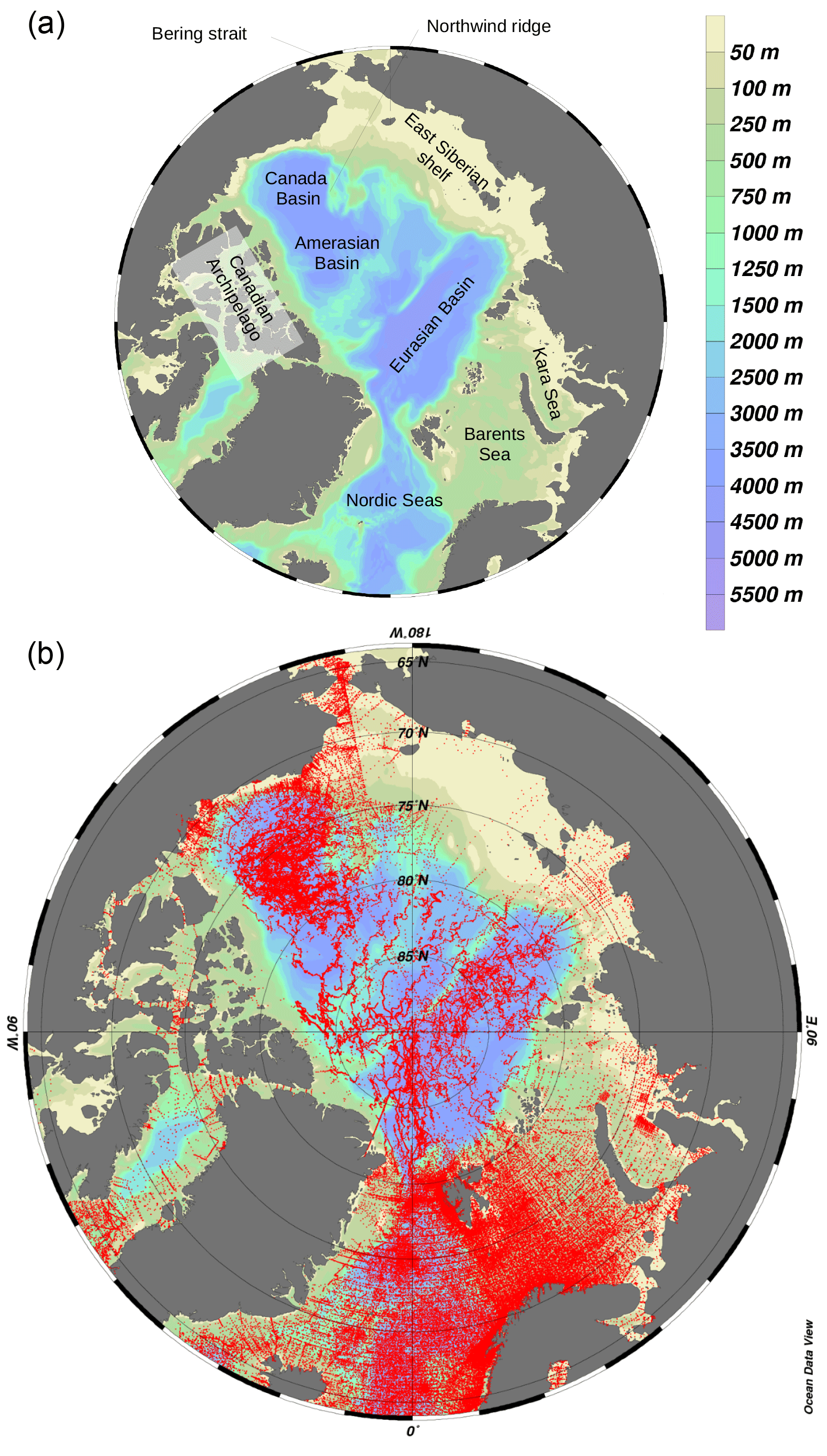
Figure 1 The topographic features of the Arctic Ocean (a) and spatial distribution of archived temperature and salinity data for the 1980–2015 period (b); a red dot is shown if there is at least one measurement in the 0–20 m depth range.

The archived information for each measurement profile includes cruise name, station number, data type, time stamp, geographical location, bottom depth (if available), measurement depth (pressure is converted to depth by the method described by Saunders, 1981), temperature, salinity, data quality information provided in the original dataset (if available), and data source information. The spatial coverage of the archived data ranges from 45^∘ N to the pole on the Atlantic Ocean side and from 64^∘ N (Bering Strait) to the pole on the Pacific Ocean side. The temporal coverage is from 1980 to 2015. Figure 1 shows an example of the spatial distribution of the archived data (0–20 m depth range, north of 64^∘ N) for the entire period. The archived data cover the entire Arctic and northern North Atlantic oceans, while the biggest data gaps are on the East Siberian Shelf and north of the Canadian Arctic Archipelago. A basic quality check is applied to the archived data before the duplication checks and statistical screening, described in the following subsections. The basic quality check is composed of (1) a bathymetric test using the merged IBCAO/ETOPO5 (Jakobsson et al., 2012) with a tolerance of 20 m, (2) a valid range test for temperature (−2.2 ^∘C $<T<\mathrm{30.0}$ ^∘C) and salinity (0 psu $<S<\mathrm{40.0}$ psu), and (3) a vertical stability test. The bathymetric test is applied to remove data with inconsistent geographic locations (i.e., either on land or indicating profile information at depths deeper than the sea floor at their location). This test excluded a number of erroneous profiles with position errors. The vertical stability test is applied to remove spike data points found in CTD and XCTD profiles. If the stability test program finds vertical density inversions, the data points are removed from the profile. If a data point violates one of the criteria, it is removed from the archive.

2.2 Duplication check

Since data obtained from various sources are prone to duplication issues, it is necessary to identify and remove duplicated data from the archive. A number of past studies, which compiled large oceanographic datasets, have suggested various automated procedures to deal with duplicate profiles (e.g., Ingleby and Huddleston, 2007; Gronell and Wijfefels, 2008; Good et al., 2013). In this study, we apply a simple duplication-check algorithm suitable for the present application. Since we are concerned only with basin-scale variability in this analysis, we count profiles that have small spatial and temporal separations as duplicates. The threshold applied for time difference between profiles is 1 day (date coincidence) and that applied for geographical location difference is 0.05^∘ in longitude and 0.01^∘ in latitude, respectively; to account for the effect of convergence of meridians toward the pole, a threshold of 2 km separation is also applied. If duplication is found (i.e., both temporal and spatial separation conditions above are met), the profiles are flagged. The profile with the highest reliability according to the data provider's own quality control is retained. For example, if we directly obtain data from PIs who have already applied their own quality-control procedure, we give the data higher priority than those from other data archives (e.g., World Ocean Database, 2013). The final duplication-checked archive is used as input for the statistical screening described below.

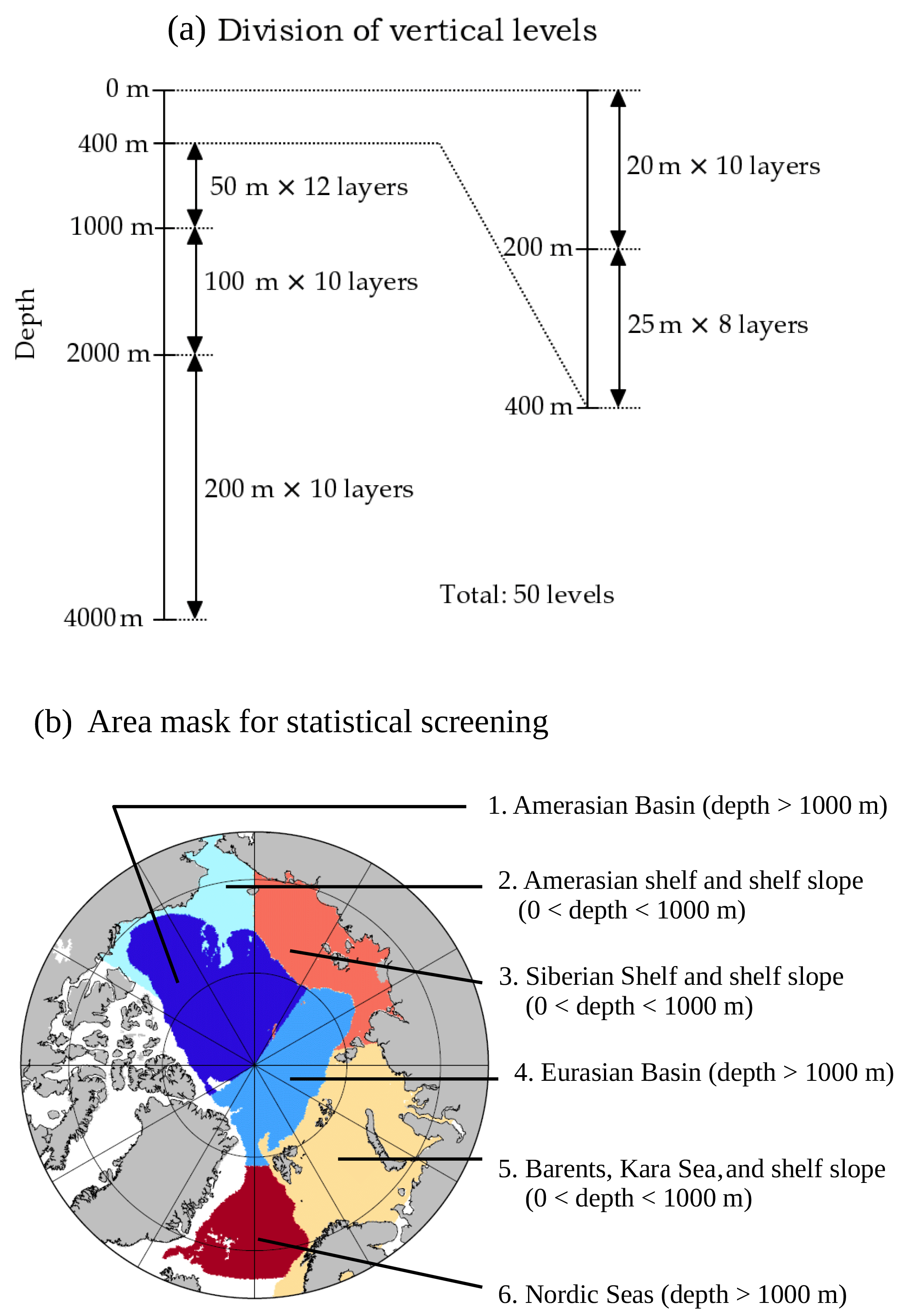
Figure 2 (a) Division of vertical levels for the statistical screening and decorrelation scale examination. The archived TS data are classified into 50 levels according to their measurement depth. Data from an identical CTD profile are averaged over each depth range and regarded as one measurement. (b) Area mask for the area-based statistical screening and the decorrelation scale examination.

2.3 Statistical screening

Since the archive contains a number of data that have not been quality controlled, we apply an additional quality-control procedure (QC) before our analyses. Note that although we describe the QC procedure as it is applied to the entire raw dataset in this section, we will use only data from 0 to 400 m depth (after the QC) in the present scale analysis as mentioned in the introduction. The QC is composed of two steps: the first step is a grid-based screening; the second step is an area-based screening. Both steps are based on statistics of the data samples in discretized depth ranges. We divide the vertical profiles of temperature (T) and salinity (S) measurements into 50 depth bins (from a 20 m interval near the sea surface to a 200 m interval in the deep ocean; Fig. 2a). If there are more than two measurements for a certain depth range from one profile, the measurement values (T and S) are averaged. The statistics are calculated and applied in each depth range separately.

First, we apply a grid-based screening. The grid-based screening takes the difference in statistics (mean and standard deviation) in different locations into account. We define 111 km × 111 km (corresponding to 1^∘ × 1^∘ at the Equator) grid cells over the entire archive domain. The mean (μ) and standard deviation (σ) of T and S on each grid cell and in each depth range are calculated from the data within the surrounding 555 km × 555 km (5^∘ × 5^∘) area. T and S values outside 5 times the standard deviation (μ±5σ) on each grid cell are removed from the archive (the procedure is repeated twice).

Second, we apply an area-based screening for the data deeper than 750 m depth. In this step, we apply more rigorous statistics calculated from the entire basin and shelf area. This step is necessary to remove problematic data in data-sparse areas and data-sparse depth ranges, since the grid-based screening cannot provide good statistics in these areas due to the small sample size (no ITP data below 750 m). We classify the archived data into six subdomains based on the characteristics of dynamical regimes (Nurser and Bacon, 2014): (1) Amerasian Basin, (2) Amerasian shelf and shelf slope, (3) Siberian Shelf and shelf slope, (4) Eurasian Basin, (5) Barents and Kara seas including their shelf slopes, and (6) Nordic Seas (Fig. 2b). Mean and standard deviation are calculated in individual subdomains. Then, data outside 5 times the standard deviation (μ±5σ) are removed (repeated twice). In this paper, we focus only on the results for the Amerasian Basin; regions 2–5 are considered in a separate analysis.

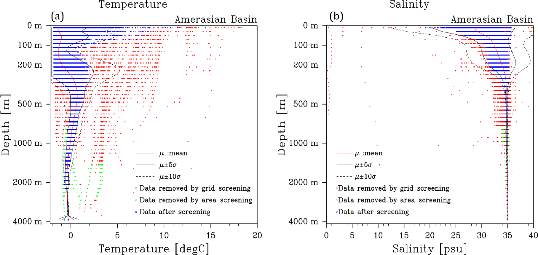
Figure 3 Temperature (a) and salinity (b) distributions versus depth (m) in the Amerasian Basin (see Fig. 2b for area definition) after a combined statistical screening. The blue dots denote data distribution after the screening, while the red (green) dots denote data removed by grid-based (area-based) statistical screening. The red line denotes the mean (μ) at each depth level after the screening, and the solid and dotted black lines indicate μ±5σ and μ±10σ, respectively. The mean and standard deviations are calculated by the data from the entire Amerasian Basin. Note that analyses in Sects. 3 and 4 use data from the 0 to 400 m depth range.

The result of the statistical screening in the Amerasian Basin is shown in Fig. 3. The combined statistical screening successfully removes spurious data in deep depth ranges, while retaining the relatively larger variability in shallow depth ranges. After the combined statistical screening, the vertically discretized data are used for the analyses in the following section.

3 Construction of the background mean field

In this section, we describe the construction of a background mean field of T and S, which represents the basin-wide climatology in the Amerasian Basin. The background mean fields will be used to calculate anomaly fields necessary for the decorrelation scale estimates. For the construction of the background mean field, we first examine the functional form and spatial scale of the mean field variation (Sect. 3.1). Second, we apply the derived functional form and scale for the background mean field construction (Sect. 3.2). The temporal linear trends of T and S are also examined to account for the effect of a long-term temporal change of the mean field (Sect. 3.3).

3.1 Spatial scale of variation

To derive the scale for the background field construction, we examine the spatial scale of variation in each depth range (the vertical layers defined in Fig. 2b are used throughout this study to provide decorrelation scales directly applicable to data assimilation systems using z-coordinate systems). In this estimation, we assume isotropy and homogeneity of the spatial scale of variation in a basin. These assumptions are valid if (1) planetary- and (2) topographic-β effects do not dominate in a basin, and (3) no dominant oceanic structure extends toward one specific direction. The first and second conditions are satisfied in the high-latitude Amerasian Basin (small planetary-β effect) away from marginal shelf slopes, where a large topographic-β effect is expected. The third condition is also satisfied in the deep Amerasian Basin, although not necessarily in other sectors of the Arctic Ocean and Nordic Seas. For example, in the Eurasian Basin, there is a prominent extension of the frontal structure along the shelf slope associated with the warm Atlantic-water inflow (Anderson et al., 1994; Rudels et al., 2013). The location of the front is not necessarily trapped over the shelf slope but can be detached from the slope (Jones, 2001). Further, in the Nordic Seas, there are meridionally extending dominant current systems, i.e., the East Greenland Current, Norwegian Current, and West Spitsbergen Current (Hopkins, 1991). These features require a scale examination that takes a spatial anisotropy into account; a different approach for scale estimation will be applied to the Eurasian Basin in a forthcoming paper. For our purposes here, the Amerasian Basin is defined by the area where total water depth is deeper than 1000 m. This definition excludes the area affected by coastal currents and topographically trapped flows (associated with the submarine Northwind Ridge, for example).

To estimate the spatial scale of variation, we introduce a structure function (Davis et al., 2008; Todd et al., 2013) with the assumption of spatial and temporal isotropy of variation,

$$\begin{array}{}\text{(1)}& {\mathit{\phi }}_{x,t}=〈{\left[\mathrm{\Omega }\left(x_{\mathrm{0}}+x,t_{\mathrm{0}}+t\right)-\mathrm{\Omega }\left(x_{\mathrm{0},}{t}_{\mathrm{0}}\right)\right]}^{\mathrm{2}}〉,\end{array}$$

where x and t are the spatial and temporal separations from location x₀ and time t₀, Ω is the observed property (in this case, either T or S), and 〈 ⋅ 〉 is the averaging operator over space and time. The structure function, φ_x, t, gives the mean square difference between two measurements as a function of spatial and temporal separations. It was initially introduced by Kolmogorov (1941) to provide a statistical description of a field without specifying the mean and variance of the field. This is an appropriate approach for the present purpose, since we do not have a priori information regarding the statistics of the background field. We calculate the structure function from all available data in the Amerasian Basin (all depth bins shallower than 400 m):

$$\begin{array}{}\text{(2)}& {\mathit{\phi }}_{x,t}=N^{-\mathrm{1}}{\sum }_{i=\mathrm{1}}^N\mathrm{\Delta }{\mathrm{\Omega }}_i{\left(x,t\right)}^{\mathrm{2}},\end{array}$$

where N is the number of available data pairs, the spatial and temporal separations of which are x and t, and ΔΩ_i (x,t) is the difference of observed values of the ith pair. We introduce a function f, which measures the normalized root mean square difference (RMSD) of any two measurements:

$$\begin{array}{}\text{(3)}& f\left(x,t\right)=\mathrm{1}-{\left({\displaystyle \frac{{\mathit{\phi }}_{x,t}}{{\mathit{\phi }}_{\text{bg}}}}\right)}^{\frac{\mathrm{1}}{\mathrm{2}}},\end{array}$$

where φ_bg is defined by all the possible combinations of available data in the basin in a certain depth range:

$$\begin{array}{}\text{(4)}& {\mathit{\phi }}_{\text{bg}}={\displaystyle \frac{\mathrm{2}}{M\left(M-\mathrm{1}\right)}}{\sum }_{i=\mathrm{1}}^{M-\mathrm{1}}{\sum }_{j=i+\mathrm{1}}^M{\left({\mathrm{\Omega }}_i-{\mathrm{\Omega }}_j\right)}^{\mathrm{2}},\end{array}$$

and M is the number of all available data. φ_bg is a measure of the size of basin-wide and long-term variations; i.e., we introduce it as the “background” mean squared difference used to normalize φ_x, t.

The function f in Eq. (3) is a unitless measure of RMSD between two measurements as a function of spatial and temporal separations. If φ_x, t ∼ φ_bg, i.e., the mean difference between two measurements with (x, t) separation is comparable to those of “large” distance measurement pairs, then f∼ 0. This indicates that no coherent structure exists between data with (x, t) separation. If ${\mathit{\phi }}_{x,t}\ll {\mathit{\phi }}_{\text{bg}}$, i.e., the mean difference between measurements with (x, t) separation is sufficiently small compared to that between sufficiently distant data pairs, then f→1. This indicates a strong coherence exists between the data with (x, t) separation (ultimately, f=1, if the spatial and temporal separations are exactly zero). Note that the function f is not an autocorrelation function, although it has similar properties (e.g., decays from 1 to 0 for spatial and temporal separations from zero to infinity). The function f measures the scale of the coherent structure of the mean field, whereas an autocorrelation function measures the scale of coherent variation of anomalies. A structure function φ can be directly related to an autocorrelation function, if we can define φ by the anomaly from the mean field (e.g., Gandin 1965; Molinari and Festa, 2000). Since we have no a priori statistical information regarding the mean field, we cannot relate the structure function φ with the autocorrelation in our case. The correspondence to the geostatistical approach is given in Appendix A.

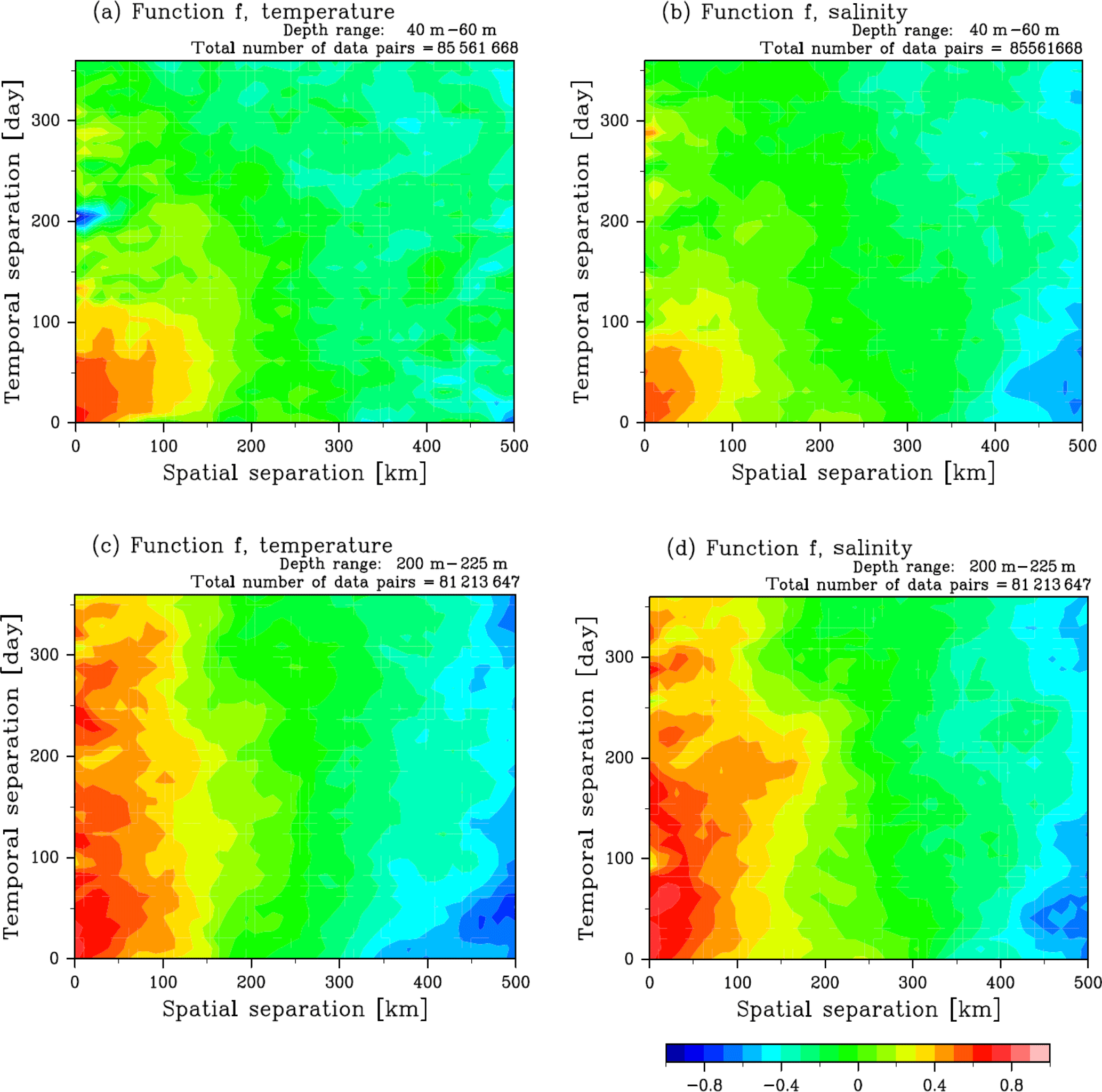
Figure 4 Function f (normalized root mean square difference) of temperature (a, c) and salinity (b, d) in 40–60 m (a, b) and in 200–225 m (c, d) depth ranges as a function of spatial (km) and temporal (days) separations of measurement pairs. The color scale is common to the panels.

In order to examine the functional form of f, we construct data pairs from all possible combinations of data in each depth range, classify the pairs into 50 × 36 bins (50 bins for spatial separation with 10 km intervals and 36 bins for temporal separation with a 10-day interval), and calculate f in respective bins. For the binning, we suppose that the spatial and temporal scales of variation are much larger than the scale used for the binning, the validity of which is recursively confirmed by the scales estimated. Examples of the functional form of f for T and S in spatial and temporal separation space are shown in Fig. 4. Small separation gives large f values, while f∼0 when the separation is sufficiently large. Note that f decays with an increase in temporal separation in shallow depth ranges with a timescale of approximately 90–120 days (Fig. 4a, b), while f is relatively insensitive to temporal separations at depths deeper than 80 m (Fig. 4c, d), which is a manifestation of the seasonality. This seasonality is taken into account to estimate the background mean field in Sect. 3.2. Note that we limit our analysis here to consider only the upper water column, from 0 to 400 m depth, as uncertainties in the uncalibrated (“level-2”) ITP salinity data are comparable to the temporal and spatial variability of salinity in the Amerasian Basin below 500 m (see Appendix B).

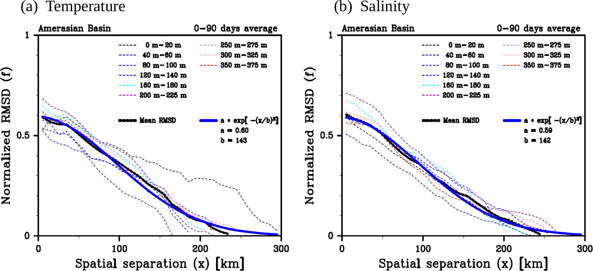
Figure 5 The 0- to 90-day temporal average of the function f (normalized RMSD) of (a) temperature and (b) salinity as a function of spatial separation. The thin-dashed lines denote functional form of RMSD in different depth levels, while the thick-solid black line in each panel denotes average of 0–400 m depth range. The thick-solid blue line is the fitted Gaussian function, $f\left(x\right)=a\times \exp [-(x/b{)}^{\mathrm{2}}]$, the fitting parameters of which are shown in each panel.

To closely examine the functional form of f, we calculate the temporal (0- to 90-day) average of f in respective depth ranges. A survey of the two-dimensional functional form over all depth ranges (shallower than 400 m) revealed that 90 days is a reasonable choice to account for seasonal variation (not shown). Figure 5 shows the 90-day averaged functional form of f in different depth ranges (thin-dotted lines) and the average for all depth ranges (0–400 m; thick-dotted black line). Although the scale of variation varies with depth, the functional form of it be reasonably approximated by a Gaussian function (thick-solid blue line). Note that f does not come close to 1, even if the spatial separation nears 0 km, because the present examination excludes self combination of data (i.e., $\mathrm{\Delta }\mathrm{\Omega }(\mathrm{0},\mathrm{0})=\mathrm{0}$), deals with a 0- to 90-day average, and does not resolve mesoscale fluctuations smaller than those at 10 km scale (the spatial separation of the bin).

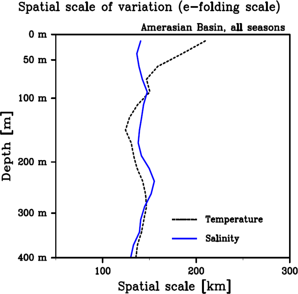
Figure 6 Vertical profile of spatial scale of variation (e-folding scale of the normalized RMSD function, f) derived from the fitted Gaussian function for each depth level (see also Fig. 5). The scale in each depth range is calculated from data from all seasons.

The e-folding scales of the fitted Gaussian function for T and S are summarized in Fig. 6. The T profile (dashed black line) exhibits a large spatial scale of variation (∼ 200 km) near the sea surface, indicating the effect of the large-scale thermal forcing at the sea surface. The T profile deeper than 100 m depth is nearly constant (120–150 km). The salinity profile (solid blue line), on the other hand, exhibits nearly constant scale (130–150 km) from the sea surface to 400 m depth, indicating small contributions from large-scale surface salinity fluxes at the sea surface. We apply the e-folding scale of each depth level and the Gaussian function to estimate the background mean field.

3.2 Background mean field

To take the seasonal variation into account, we divide the observed data into four seasons (January–March, April–June, July–September, and October–December), and construct the background mean T and S fields in each season. This is supported by the fact that the temporal e-folding scale is approximately 90 days in shallow layers (Fig. 4a, b) and even longer in the deeper layers. The background field is derived by applying a spatial Gaussian filter with an e-folding scale given by the spatial scale of variation in each depth range (Fig. 6). The background field for Ω_i is given by

$$\begin{array}{}\text{(5)}& ={\sum }_{n=\mathrm{1}}^N{W}_n^{\prime }{\mathrm{\Omega }}_n,\end{array}$$

where N is the number of measurements, whose distance from the ith measurement (Ω_i) is less than 3 times the e-folding scale (i.e., $\Vert x_i-x_n\Vert <\mathrm{3}L$; see below), $W_n^{\prime }$ is the normalized weighting function for the nth data point, and Ω_n is the nth measurement surrounding the ith measurement. The normalized weighting function $W_n^{\prime }$ is given by

$$\begin{array}{}\text{(6)}& W_n^{\prime }={\left({\sum }_{n=\mathrm{1}}^N{W}_n\right)}^{-\mathrm{1}}{W}_n,\end{array}$$

where W_n is the Gaussian weighting function:

$$\begin{array}{}\text{(7)}& W_n=\exp \left[-{\left({\displaystyle \frac{∥x_i-x_n∥}{L\left(z\right)}}\right)}^{\mathrm{2}}\right],\end{array}$$

where x_i and x_n are the geographical location of Ω_i and Ω_n, respectively, and L(z) is the e-folding scale of the Gaussian filter as a function of depth (Fig. 6). An example of the derived background field for T and S in summer is shown in Fig. 7. The field captures a warm and fresh water mass distribution in the Canada Basin and its smooth transition toward cold and saline water in the northeastern Amerasian Basin. For the anomaly field calculation, we require the background field at the locations where observational data exist. Therefore, we do not apply any spatial and/or temporal interpolations even in data-sparse seasons (winter and spring).

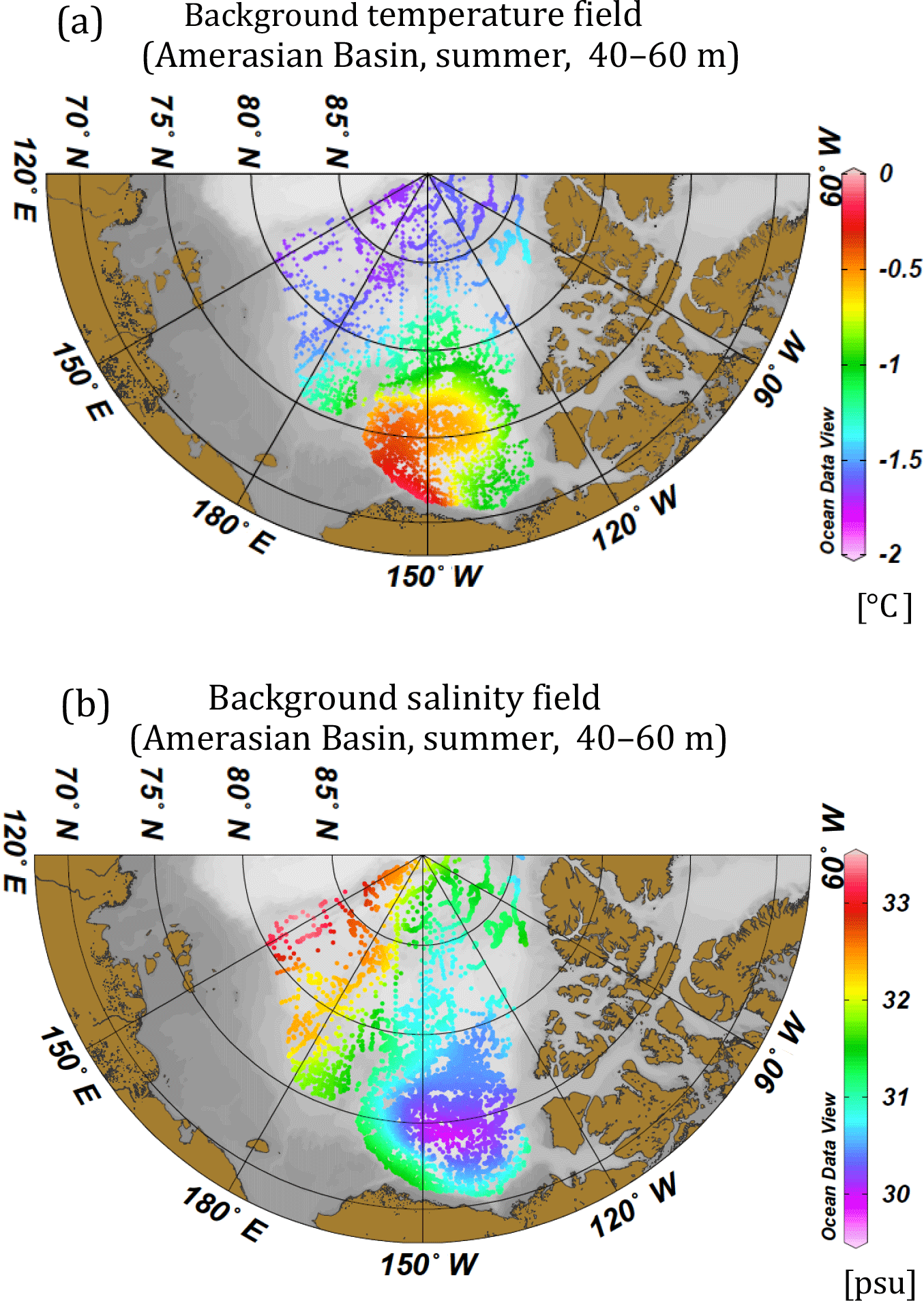
Figure 7 Background mean field of (a) temperature and (b) salinity (40–60 m depth range) in summer (July–September) obtained by Gaussian filtering with the e-folding scales shown in Fig. 6. A vertical filter (average of three adjacent layers) is applied to the e-folding scales before the application in order to obtain a smooth transition of the filtering scale in the vertical direction. The background field is calculated only at the locations where data exist in the Amerasian Basin (bottom depth >1000 m).

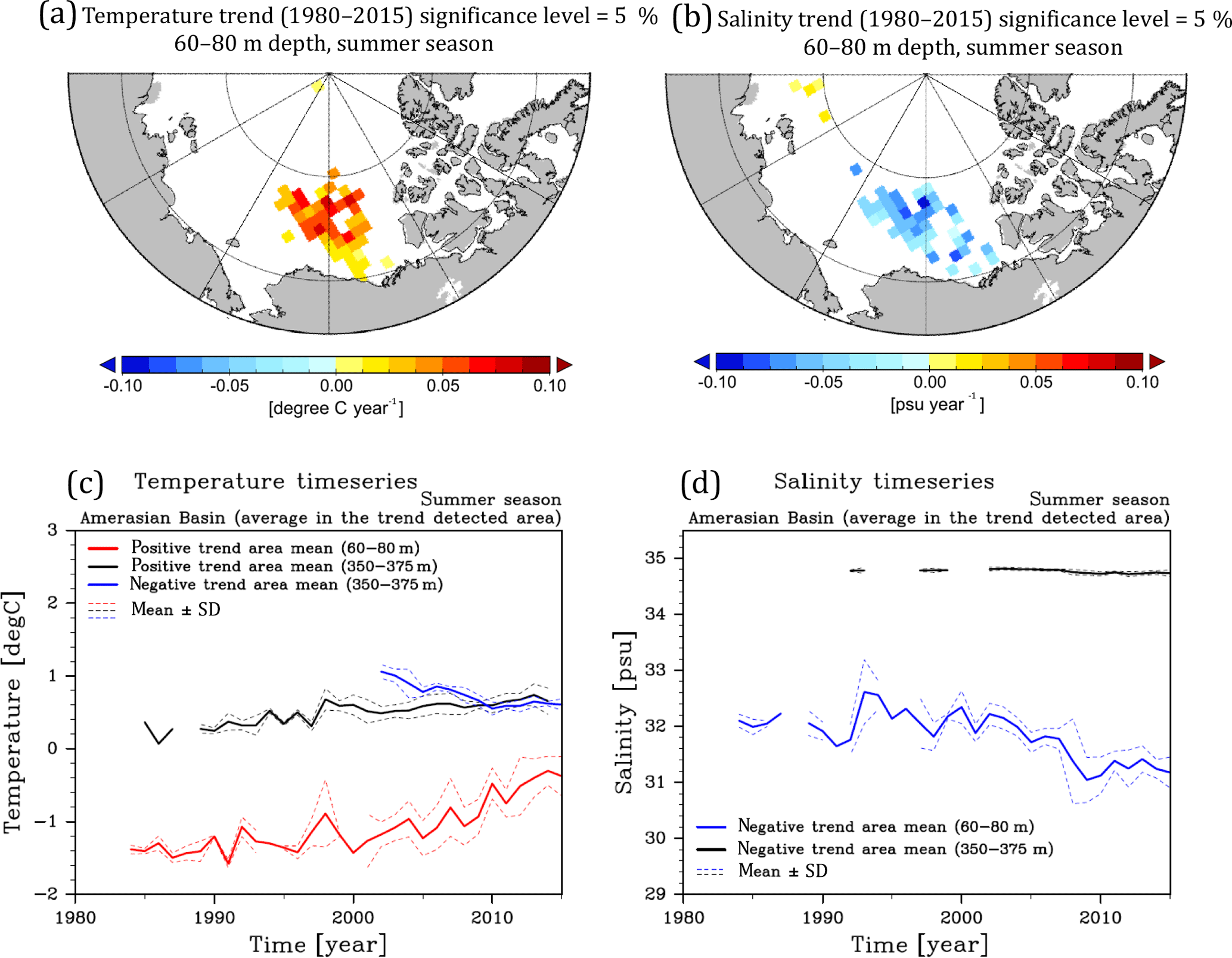
Figure 8 A summary of linear temporal trend in the Amerasian Basin: the spatial pattern of (a) temperature and (b) salinity trend in 60–80 m depth range, and the time series of averaged (c) temperature and (d) salinity over the grid cells where a trend is detected in the Amerasian Basin. The trend is calculated in each 111 km × 111 km grid cell for the period covered by data, and the Mann–Kendall rank statistic (Kendal, 1938) is applied to test the significance. In panels (a) and (b), only the grid cells, the trends of which are statistically significant (significance level 5 %), are shown in color. Time series of averaged temperature/salinity over the corresponding area are shown in panels (c) and (d) by the thick-solid lines. Black thick-solid lines in panels (c) and (d) exhibit averages over the grid cells, where positive (negative) trends of T (S) are detected along the southern perimeter of the Canada Basin in the 350–375 m depth range (spatial pattern is not shown). The dashed lines in panels (c, d) depict the range of 1 standard deviation.

3.3 Temporal trend

For the present anomaly derivation, we also take the temporal trend from 1980 to 2015 into account. The trend is estimated in each 111 km × 111 km grid cell (1^∘ × 1^∘ at Equator scale), in each depth range, and in each season (Mann–Kendall rank statistics; Kendall, 1938) with a significance level of 5 %). The size of the grid cells is chosen to be consistent with the spatial scale of variation (Sect. 3.2). Figure 8 shows representative T and S trends in the 60–80 m depth range in summer and the corresponding average time series for those grid cells for which the trend is statistically significant. A warming (∼ 0.5 ^∘ decade⁻¹) and freshening (∼ 0.5 psu decade⁻¹) trend in the Canada Basin is evident in this depth range. The freshening trend extends from the sea surface to 400 m depth without a significant change in spatial pattern, whereas the T trend changes sign and spatial pattern with depth. A positive trend in T is observed in the depth range from 0 to 160 m over the whole analyzed time period (i.e., through the Pacific-water/upper halocline layers, represented by red line in Fig. 8c), while after the year 2002 a decreasing trend in T is observed in the central Canada Basin in the 200–400 m depth range (lower halocline/Atlantic-water layer, represented by blue line in Fig. 8c). A positive trend is observed along the southern perimeter of the Canada Basin in 250–400 m depth range (Atlantic-water layer, represented by black line in Fig. 8c and d).

The warming and freshening trend in the Pacific-water layer has already been reported by many studies (e.g., Proshutinsky et al., 2009; Jackson et al., 2010; Giles et al., 2012; Timmermans et al., 2014). The cooling trend in the central Canada Basin and the warming trend along its southern perimeter are a consequence of deepening of the warm Atlantic water in the central basin and concurrent upwelling of warm Atlantic water at the boundaries, a manifestation of an intensification of the anticyclonic Beaufort Gyre in recent years (e.g., McLaughlin et al., 2009; Karcher et al., 2012; Zhong and Zhao, 2014). Although similar trends can be found in other seasons (from winter to spring), they are not statistically significant.

The temporal trend in each location is used to define a time-varying background field. Since the temporal distribution of the archived data is not spatially uniform, the representative time (i.e., the time that the temporal mean value represents) of the background field ${\stackrel{\mathrm{‾}}{\mathrm{\Omega }}}_i$ varies with space. The representative time is used as a tie point (offset) to connect the mean and trend. Taking the effect of the representative time into account, the time-varying background field for Ω_i is defined by

$$\begin{array}{}\text{(8)}& {\stackrel{\mathrm{̃}}{\mathrm{\Omega }}}_i=a\left(x\right)\left[t-t_{\text{rep}}\left(x\right)\right]+{\stackrel{\mathrm{‾}}{\mathrm{\Omega }}}_i,\end{array}$$

where a(x) is the temporal trend at location x, t is the time, t_rep(x) is the representative time of the background mean field ${\stackrel{\mathrm{‾}}{\mathrm{\Omega }}}_i$ at location x. We calculate the representative time in each 111 km × 111 km area by the average of measurement times of all the data contained in the corresponding area and apply it to define the time-varying background field (see the Supplement). For the area where no trend can be deduced, we apply a constant background field, ${\stackrel{\mathrm{̃}}{\mathrm{\Omega }}}_i={\stackrel{\mathrm{‾}}{\mathrm{\Omega }}}_i$.

4 Decorrelation scale

4.1 Autocorrelation function

Decorrelation scales used in oceanographic studies are generally defined by an e-folding scale of an autocorrelation function, which has a Gaussian or exponential functional form (Molinari and Festa, 2000). Practically, the autocorrelation functions are obtained from a series of autocorrelations estimated by differently lagged points (e.g., White and Meyers, 1982; Meyers et al., 1991). An autocorrelation for Δl lag is given by

$$\begin{array}{}\text{(9)}& {\mathit{\rho }}_{\mathit{l},\mathit{l}+\mathrm{\Delta }\mathit{l}}={\displaystyle \frac{\text{cov}\left({\mathbf{\Omega }}_{\mathit{l}},{\mathbf{\Omega }}_{\mathit{l}+\mathrm{\Delta }\mathit{l}}\right)}{\sqrt{\text{var}\left({\mathbf{\Omega }}_{\mathit{l}}\right)\cdot \text{var}\left({\mathbf{\Omega }}_{\mathit{l}+\mathrm{\Delta }\mathit{l}}\right)}}},\end{array}$$

where cov(Ω_l, Ω_l+Δl) is an autocovariance between two data series Ω_l and Ω_l+Δl, the temporal and/or spatial lag between which is Δl, and var(Ω_l) and var(Ω_l+Δl) are the variances of Ω_l and Ω_l+Δl, respectively. We assume isotropy and homogeneity of the autocorrelation in the Amerasian Basin, supported by the weak planetary-β effect in polar regions and the homogeneity of the Rossby radius in the Amerasian Basin (Nurser and Bacon, 2014; Zao et al., 2014). These assumptions enable us to calculate the autocorrelation from data series, which are composed of data pairs having the same temporal and spatial lag Δl but come from different locations in the basin and from different times (e.g., Sprintall and Meyers, 1991; Chu et al., 1997, 2002), i.e.,

$$\begin{array}{}\text{(10)}& {\mathit{\rho }}_{\mathrm{\Delta }\mathit{l}}={\displaystyle \frac{{\sum }_{n=\mathrm{1}}^N{{\mathrm{\Omega }}^{\prime }}_n{{\widehat{\mathrm{\Omega }}}^{\prime }}_n}{\sqrt{{\sum }_{n=\mathrm{1}}^N{\left({{\mathrm{\Omega }}^{\prime }}_n\right)}^{\mathrm{2}}\cdot {\sum }_{n=\mathrm{1}}^N{\left({{\widehat{\mathrm{\Omega }}}^{\prime }}_n\right)}^{\mathrm{2}}}}},\end{array}$$

where N is the number of data pairs, the spatial and temporal lags between which are Δl, ${\mathrm{\Omega }}_n^{\prime }$ is the anomaly value of the nth data, ${{\widehat{\mathrm{\Omega }}}^{\prime }}_n$ is the anomaly value of the paired data which locates Δl-lagged point from ${\mathrm{\Omega }}_n^{\prime }$.

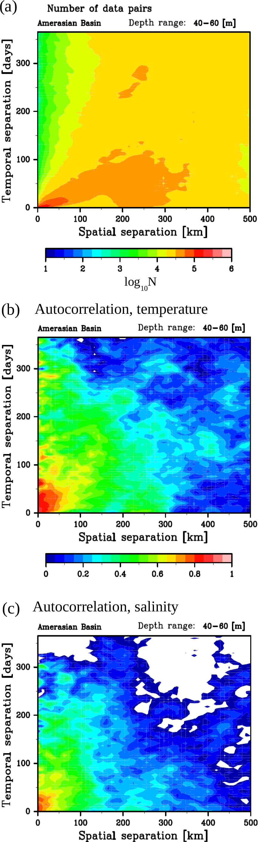
Figure 9 (a) Number of data pairs used to calculate autocorrelation in each bin (log-scale) and two-dimensional autocorrelation function for (b) temperature and (c) salinity in 40–60 m depth range. The color bar for panel (b) is common to (c). The white area in panels (b) and (c) indicates negative autocorrelations.

The anomaly dataset Ω^′ is defined by subtracting the time-varying background field $\stackrel{\mathrm{̃}}{\mathbf{\Omega }}$ from the observed data Ω. Each anomaly datum of the set is paired with the other anomalies to construct a set of anomaly data pairs, which consists of all possible combinations of two anomaly data. The data pairs are classified into discretized bins, according to the spatial and temporal lags of the paired data (50 spatial bins with a 10 km interval and 73 temporal bins with a 5-day interval; i.e., the examination window is 500 km lag × 365-day lag). The spatial and temporal sizes of the bin are designed to capture the functional form of the autocorrelation relevant for basin-scale data assimilation (i.e., the functional form of the autocorrelation describing mesoscale fluctuations are not examined in this analysis). Each bin has a sufficient number of data pairs to calculate an autocorrelation (N>O(10³); see Fig. 9a). Figure 9b, c show examples of the autocorrelation functions for T and S in the 40–60 m depth range. There is a clear decrease of autocorrelation with increasing spatial and temporal lags, although with some variability about this relationship.

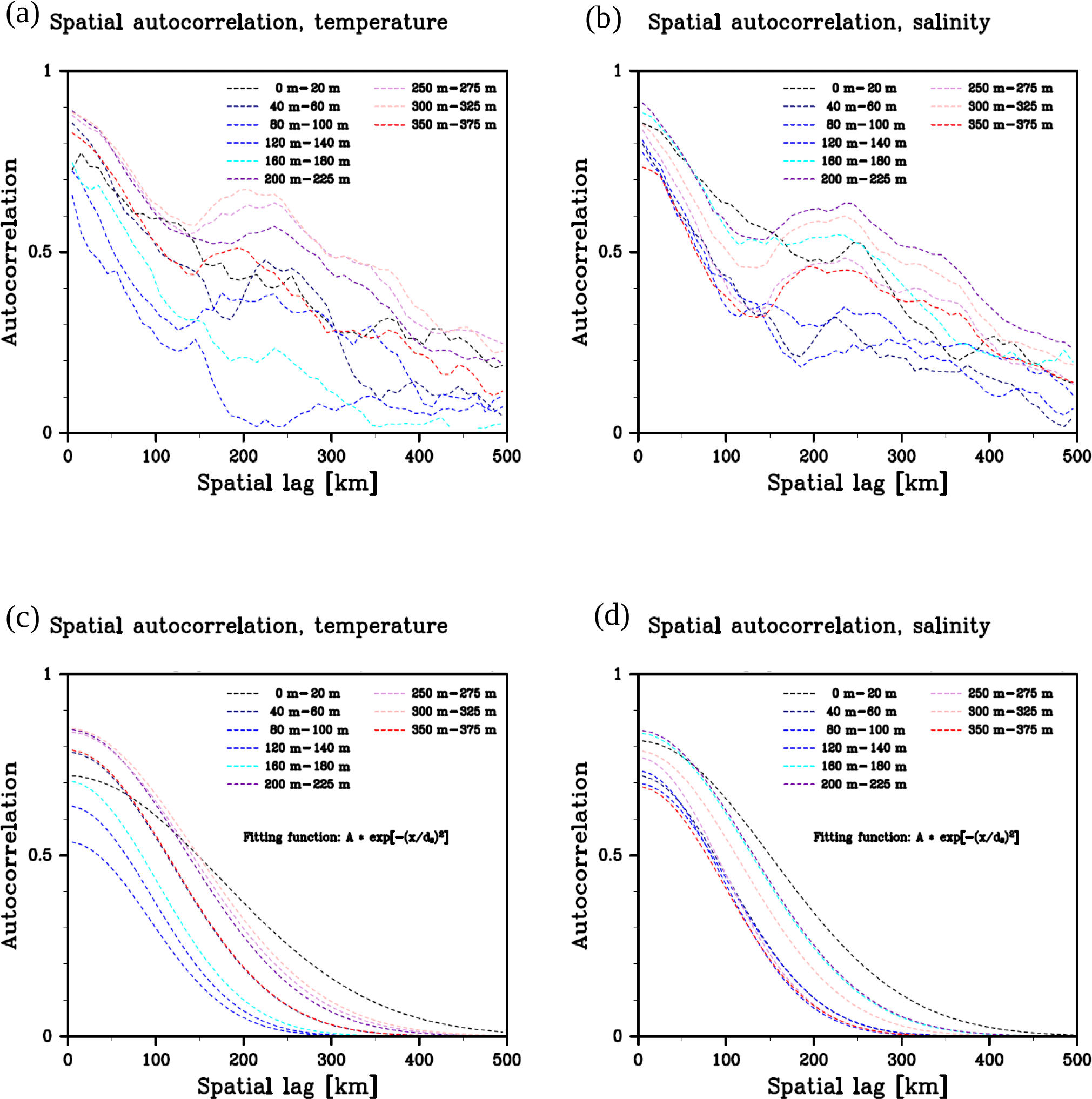
Figure 10 Spatial autocorrelation function of temperature (a, c) and salinity (b, d). The upper panels show the temporal averages of the two-dimensional autocorrelation functions (the average of the 0- to 30-day lag for the 0–140 m depth range, 0- to 60-day lag for the 140–400 m depth range) in various depth levels. The lower panels are Gaussian functions, the intercepts and e-folding scales of which are calculated from the function fitting in the 0–150 km spatial-lag range.

Temporal and spatial averages of the autocorrelation are calculated to identify its functional form by fitting a suitable empirical function. Figure 10a and b show the temporal average of the spatial autocorrelation functions of T and S for different depth ranges. To account for the effect of differences of temporal autocorrelation scales in different depth ranges, we define the temporal average by a 0- to 30-day lag in shallow levels (0–140 m depth range) and by a 0- to 60-day lag in deeper levels (below 140 m). The functions generally show their highest values at zero-spatial lag, with decreasing values as the spatial lag increases. Some functions exhibit a second peak around a spatial lag of 200–300 km. We examine the relation between the second peaks and associated background mean field of T and S in different depth ranges, and find that the peaks derive from the circular T and/or S structure of the Beaufort Gyre (see Appendix C). Since the Beaufort Gyre is characterized by bowl-shaped isosurfaces of T and S associated with surface downward Ekman pumping, coherent variation of the isosurfaces gives rise to the second peak. To eliminate the effect of the second peak for our scale estimate, we use the autocorrelation functions just for a spatial lag of 0–150 km to compute a fitting function. We tested exponential and Gaussian functions for the fitting and found that the Gaussian function is generally suitable to represent the observationally derived spatial autocorrelations (Fig. 10c, d).

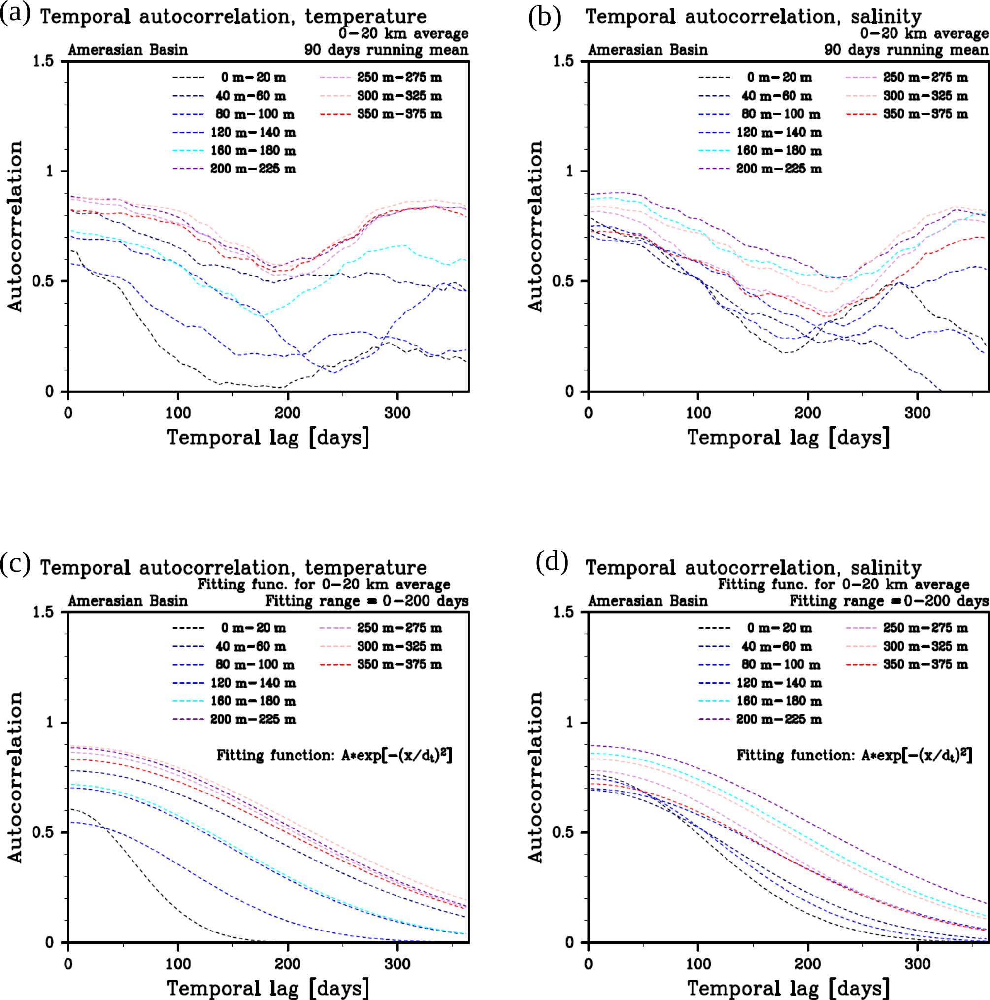
Figure 11 Temporal autocorrelation function of temperature (a, c) and salinity (b, d). The upper panels show the spatial averages of the two-dimensional autocorrelation functions (the spatial average of 0–20 km lag) in various depth levels. The lower panels are Gaussian functions, the intercepts and e-folding scales of which are calculated from the function fitting in a 0- to 200-day temporal-lag range. A 90-day temporal filter is applied to the autocorrelation functions in panels (a) and (b) to eliminate noise.

The temporal autocorrelation is also examined by taking spatial-lag averages (0–20 km) of the two-dimensional autocorrelations of T and S. Figure 11a, b show the averaged temporal autocorrelation functions in various depth ranges. The functions show their highest values at zero-temporal lag and a reduction towards large temporal lags, whereas the functions from many depth ranges clearly exhibit an annual cycle. Since the seasonal variability of the background field is already taken into account (Sect. 3.2), the annual cycle found in the temporal autocorrelations indicates the effect of persistent atmospheric forcing, the timescale of which is longer than 1 year (e.g., Arctic Oscillation, Thompson and Wallace, 1998; North Atlantic Oscillation, Hurrell, 1995; Wallace, 2000), and/or spin-up/-down process of gyre-scale circulation, the timescale of which is estimated as 3–4 years (Yoshizawa et al., 2015). To remove the effect of the annual cycle found in Fig. 11a, b, we use the autocorrelation functions from 0 to 200 days of temporal lag to find a fitting function for the temporal autocorrelation. We again tested exponential and Gaussian forms for the fitting, and found that the Gaussian functions are suitable to represent the form of the temporal autocorrelation functions (Fig. 11c, d).

4.2 Decorrelation scale

The spatial and temporal decorrelation scales of T and S are derived from the e-folding scales of the fitted spatial and temporal autocorrelation functions in the respective depth ranges. The spatial autocorrelation function is represented by the Gaussian form,

$$\begin{array}{}\text{(11)}& {\mathit{\rho }}_{\mathrm{s}}=A_{\mathrm{s}}\cdot \exp \left[-{\left({\displaystyle \frac{x}{d_{\mathrm{s}}}}\right)}^{\mathrm{2}}\right],\end{array}$$

where A_s is the autocorrelation at zero-spatial lag, x is a spatial lag, and d_s is the spatial decorrelation scale. The temporal autocorrelation function has the same formula but exchanges A_s for A_t, x for t, and d_s for d_t, where A_t, t, and d_t are the autocorrelation at zero-temporal lag, temporal lag, and temporal decorrelation scale, respectively. The autocorrelation at zero-temporal and -spatial lag (A_s and A_t) represents the effect of unresolved fluctuations, which have a scale smaller than the resolution of the present analysis at 10 km resolution in space and 5-day resolution in time (1–A_s represents the magnitude of unresolved fluctuations relative to the basin-scale fluctuations). The effect of mesoscale eddies with the scale of the deformation radius (order of 10 km horizontally) is described by this parameter.

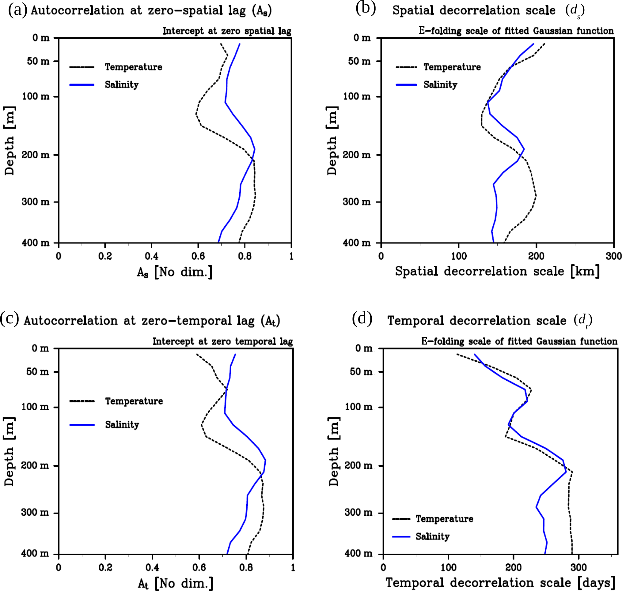
Figure 12 Vertical profiles of zero-lag autocorrelation (a, c) and e-folding scale (b, d) of the fitting spatial (a, b) and temporal (c, d) autocorrelation functions. A three-layer vertical filter is applied to eliminate noise.

Figure 12 summarizes the vertical profiles of the spatial and temporal decorrelation scales (d_s and d_t) of T and S with the associated parameters for zero-lag autocorrelations (A_s and A_t). The zero-lag autocorrelations (Fig. 12a, c) show smaller values (0.6–0.7) in the upper 100 m depth range, indicating active mesoscale processes (e.g., eddy activity observed in the Pacific-water layer; e.g., Zhao et al., 2014). The zero-lag autocorrelations for spatial (Fig. 12a) and temporal lags (Fig. 12c) exhibit similar profiles, confirming the appropriateness of the spatial and temporal averages used for the functional form examinations. The vertical profiles of the decorrelation scale (Fig. 12b, d) indicate an influence of the sea surface boundary condition at shallow levels. The spatial decorrelation scale near the sea surface (∼ 200 km) is larger than it is in deeper layers (∼ 150 km), as a consequence of the direct influence of the atmosphere and sea ice, the spatial scale of which is larger than the scale of intrinsic ocean processes. The temporal decorrelation scale near the surface (100–150 days), on the other hand, is shorter than that of the deeper layers (200–300 days), possibly due to the effect of short-timescale variation of the atmospheric field and associated sea-ice motion. It is interesting to note that the scales of the mean field and of the variance are very similar (e.g., compare Figs. 6 and 12b). We currently have no explanation for this feature but assume that it is a peculiarity based on the dynamics of the analyzed basin. In forthcoming papers, we plan to analyze the scales in the Eurasian basin and over the Arctic shelf slope and will revisit this question.

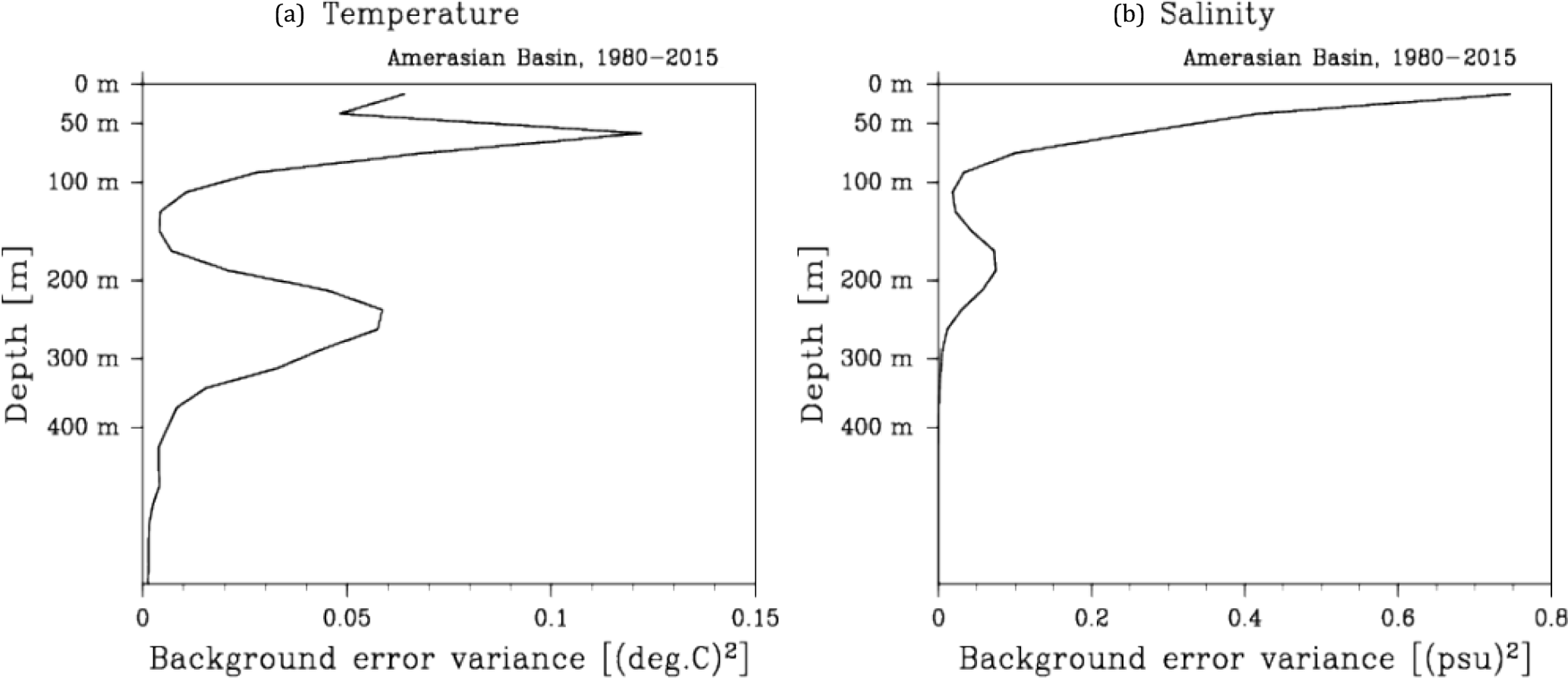
Figure 13 Vertical profile of the background mean variance, var_bg, for temperature (a) and salinity (b).

Note that the T and S profiles exhibit similar vertical profiles in the depth range shallower than 250 m, while discrepancies stand out in levels deeper than 250 m (Fig. 12b, d). This may be due to small calibration errors associated with our use of ITP level-2 (i.e., not the fully calibrated level-3) data (see Krishfield et al., 2008b; Johnson et al., 2007). In order to incorporate as many data as possible, we have included all available ITP level-2 data, where level-3 data are not yet available. This strategy is beneficial for scale estimation of temperature (ITP level-2 temperature data have the same accuracy as level-3 data, within ±0.001 ^∘C) in the entire depth range and salinity shallower than 250 m depth. On the other hand, since salinity variability decreases with depth (Fig. 3b), the uncalibrated ITP level-2 salinity data may yield non-negligible spurious variation at levels deeper than 250 m, which may deteriorate the accuracy of the scale estimates for salinity in this depth range.

4.3 Error covariance

The autocorrelation function derived in Sect. 4.1 can be related to an error covariance by Eq. (9). Since the variance in Eq. (9) used to normalize the covariance does not depend on spatial and/or temporal separation in principle (see the assumption in Sect. 4.1), it can be represented by a variance calculated from all the data in the Amerasian Basin. Therefore, the error covariance associated with the representation error is given by a function of spatial and temporal separations, x and t:

$$\begin{array}{}\text{(12)}& \text{cov}\left(x,t\right)=\mathit{\rho }\left(x,t\right)\cdot {\text{var}}_{\text{bg}},\end{array}$$

where ρ(x, t) is the autocorrelation function, and var_bg is the background mean variance defined by

$$\begin{array}{}\text{(13)}& {\text{var}}_{\text{bg}}={\displaystyle \frac{\mathrm{1}}{M}}{\sum }_{i=\mathrm{1}}^M{\left({\stackrel{\mathrm{̃}}{\mathrm{\Omega }}}_i-{\mathrm{\Omega }}_i\right)}^{\mathrm{2}}.\end{array}$$

The vertical profiles of var_bg for T and S are shown in Fig. 13. The background mean variance clearly reflects the vertical stratification in the Amerasian Basin (e.g., McLaughlin et al., 2004; Shimada et al., 2005), with highest variance in the depth ranges of vertical extrema in the profile. The temperature profile exhibits two minima (in the mixed layer and around 130 m depth) and two maxima (approximately in 70 and 250 m; Fig. 3a). These shallow extrema are associated with the seasonally, spatially, and interannually varying near-surface temperature maximum (see, e.g., McPhee et al., 1998), and Pacific summer water layers (see, e.g., Timmermans et al., 2014). The deep minimum corresponds to the Pacific winter water layer plus variations in the deeper Atlantic water (see, e.g., Shimada et al., 2005; Fig. 2). The vertical profile of salinity variance also exhibits good correspondence with salinity stratification and its variation (Fig. 3b), with smallest variance (approximately 120 m depth) corresponding to weakest salinity stratification and largest (around 180 m) corresponding to the stratification boundary between the upper and lower halocline. The derived covariance is also necessary to complete the model– observation misfit calculation, as summarized in the following section.

5 Conclusions

We examined spatial and temporal scales of T and S anomalies from the mean fields in the Amerasian Basin. To provide scales describing the anomalies, we examined the autocorrelation of T and S measurements and calculated spatial and temporal decorrelation scales. Historical T and S measurements in the Arctic and northern North Atlantic oceans were compiled for this study and for future applications to Arctic Ocean data assimilations. The resulting quality-controlled archive was used to construct a background mean field, from which anomaly fields were derived. By assuming spatial and temporal homogeneity of the autocorrelation function in the basin interior, we calculated autocorrelations as a function of spatial and temporal lags. The examination revealed that the autocorrelation function can be well described by a Gaussian function in space and time. The spatial and temporal decorrelation scales were estimated to be 150–200 km in space and 100–300 days in time (e-folding scales of the autocorrelation function). The spatial decorrelation scale is relatively large near the sea surface, while the temporal scale is relatively small near the surface. Mesoscale fluctuations, with scales smaller than 10 km and shorter than 5 days, are represented by the zero-lag autocorrelation. The zero-lag autocorrelation should be re-examined in future work to describe the autocorrelation smaller than the Rossby radius by fully exploiting ITP data.

The estimated function and the scales, together with the associated error covariance, are directly applicable to model–observation misfit calculation in data assimilation systems, which intend to assimilate a spatially and temporally varying field. A cost function measuring the model–observation misfit is given by

$$\begin{array}{}\text{(14)}& J={\displaystyle \frac{\mathrm{1}}{\mathrm{2}}}{\left[\mathit{d}-H\left(\mathit{m}\right)\right]}^T{\mathbf{R}}^{-\mathrm{1}}\left[\mathit{d}-H\left(\mathit{m}\right)\right],\end{array}$$

where d is the data vector, m is the model vector, H is the observation operator, and R is the observation error covariance matrix. The current study gives the descriptive form of H and R. An observation operator, H, which takes spatial and temporal representativeness of each measurement into account, is given as follows:

$$\begin{array}{}\text{(15)}& H_i\left(\mathit{m}\right)={\displaystyle \frac{{\sum }_{j=\mathrm{1}}^M{m}_j\mathit{\rho }\left(x_{ij},t_{ij}\right)}{{\sum }_{j=\mathrm{1}}^M\mathit{\rho }\left(x_{ij},t_{ij}\right)}},\end{array}$$

where i refers to the ith in situ measurement, j refers to the modeled variable at the jth model grid point, ρ is the autocorrelation between (x, t)-distant locations, x_ij and t_ij are the spatial and temporal separations between the ith measurement and the jth model grid point. The operator H_i(m) maps the model field m to the ith measurement location (in space and time), in accordance with the influence of the measurement. We can describe the autocorrelation function ρ by the results shown in Sect. 4.1 and 4.2 in the following formula:

$$\begin{array}{}\text{(16)}& \mathit{\rho }(x,t)=A\cdot \exp \left[-{\left({\displaystyle \frac{x}{d_{\mathrm{s}}}}\right)}^{\mathrm{2}}-{\left({\displaystyle \frac{t}{d_{\mathrm{t}}}}\right)}^{\mathrm{2}}\right],\end{array}$$

where A is the autocorrelation between zero-lag locations (x<10 km and t<5 days) representing the contributions from unresolved-scale fluctuations (Fig. 12a); d_s and d_t are the spatial and temporal decorrelation scales (Fig. 12b, d), respectively. This formula provides the representation error of a point measurement at (x, t)-distant locations. Note that the current formula enables us to quantify errors of modeled T and S not only at the location where the measurements exist but also at the locations distant from the measurements. The present study also provides error covariance matrix R associated with the representation error. The representation error covariance between the ith and the i^′th measurements is

$$\begin{array}{}\text{(17)}& \text{cov}\left(i,i^{\prime }\right)=\mathit{\rho }\left(x_{i{i}^{\prime }},t_{i{i}^{\prime }}\right)\cdot {\text{var}}_{\text{bg}},\end{array}$$

where $\mathit{\rho }(x_{i{i}^{\prime }}$, $t_{i{i}^{\prime }})$ is the autocorrelation between ith and i^′th measurements, the spatial and temporal separations between which are given by $x_{i{i}^{\prime }}$ and $t_{i{i}^{\prime }}$, and var_bg is the background error variance given as a function of depth (Fig. 13). As summarized here, the current study provides a full descriptive formula to exploit ocean in situ measurements in the Amerasian Basin for a model–observation misfit calculation.

The present scale estimates pose a requirement from a basin-scale data assimilation on a sampling strategy. Static interpolation approaches (e.g., optimal interpolation (Gandin, 1965; Reynolds and Smith, 1994), objective mapping (Wong et al., 2003; Böhme and Send, 2005; Böhme et al., 2008), and data-interpolating variational analyses (Troupin et al., 2010, 2012; Korablev, 2014) exploit statistical information of data to derive a mean analysis field. Data assimilation approaches, in addition, exploit modeled physics and provide temporally and spatially varying four-dimensional analysis fields. The former approaches need a scale representing the mean field, while the latter, in addition, needs spatial and temporal scales representing the anomaly field to fully exploit the information embedded in in situ data. For Arctic Ocean studies, statistical interpolation has been using decorrelation scales of 300–500 km (Steele et al., 2001; Proshutinsky et al., 2009; Rabe et al., 2011, 2014), while the present study suggests the necessity of a smaller measurement interval (150–200 km in space and 100–300 days in time) to describe the anomaly field by a basin-scale data assimilation.

Further studies are necessary to interpret the decorrelation scale of S and T in the context of ocean dynamics and relate it to the hydrographic features in the Amerasian Basin. The scale of ocean variability is governed by external forcings and by various physical processes in the ocean. The local dynamic response to local external forcing (i.e., vertical normal mode in response to basin-scale wind stress curl; Pedlosky, 1987; Olbers et al., 2012) is one very likely mechanism to explain the shape of the vertical profile of the scale. Near the sea surface, the decorrelation scales should be examined in relation to the scale of atmosphere and sea-ice variability (Walsh, 1978; Walsh and Chapman, 1990), and the dynamical processes governing the mixed layer (Peralta-Ferriz and Woodgate, 2015). The effect of remote forcing is another important issue to be examined. Advection of anomalous water masses introduces scales governed by mechanisms outside of the basin and/or shelf–basin interaction, such as the inflow of anomalous Pacific water into the deep basin (Steele et al., 2004; Itoh et al., 2012), its modification processes on the shelf (Pickart et al., 2005, Woodgate et al., 2005), the advection of anomalous Atlantic water (McLaughlin et al., 2009; Karcher et al., 2012), or variations of freshwater supply due to river runoff (Lammers et al., 2001). In this study, we employed level surfaces, as we focus on the applicability of the decorrelation scales for model validation and data assimilation (many models use the so called z-coordinate system). For future studies which aim at a dynamical interpretation of the decorrelation scales, an analysis in isopycnal coordinates would be a logical next step. Autocorrelation and decorrelation scale estimates for other parts of the Arctic Ocean (i.e., the Eurasian Basin and over the shelf slopes) will be presented in forthcoming papers.

Appendix A: Correspondence to the geostatistical approach

Since data analysis software based on geostatistical approaches (e.g., iSATiS, SURFER) is used in oceanographic studies in recent years, it is useful for providing a summary of the relation between the current approach and geostatistical approaches. The spatial scale of variation estimated in Sect. 3.1 is a different notation of the variogram concept used in geostatistics. In the present formula, we normalize the variance by the sill of the variogram, and a root-squared value is considered. This is because a variogram deals with a variance (i.e., spatial scale of the squared difference between two measurements), while we intend to quantify the spatial scale of difference between two measurements. We also defined the function by the value subtracted from 1, in order to obtain a function decaying to zero at infinity. This is done for mathematical convenience in order to obtain a Gaussian-like function. This is preferable for the framework of the best linear unbiased estimator (BLUE), which is constituting the basis of data assimilation theories. Since the spatial scale of variation originates from the same concept as variograms, it can be related to the terminology used in geostatistical approaches. The function f (i.e., normalized root mean square difference) at zero separation (Fig. 5) is

$$\begin{array}{}\text{(A1)}& f{\mathrm{|}}_{x=\mathrm{0}}=\mathrm{1}-\sqrt{{\displaystyle \frac{\mathrm{2}{N}_g}{{\mathit{\phi }}_{\text{bg}}}}},\end{array}$$

where N_g is a nugget of the semivariogram plot. The estimated scale (the spatial scale of variation) describes the square root of the scale described by a variogram, although it is not easy to find an exact correspondence, since empirical functions describing the two functions may differ. If we directly translate the function f into a semivariance used to plot a semivariogram, our formulation corresponds to an empirical semivariance with the following form:

$$\begin{array}{}\text{(A2)}& \widehat{\mathit{\gamma }}\left(x\right)={\displaystyle \frac{{\mathit{\phi }}_{\text{bg}}}{\mathrm{2}}}{\left[A{e}^{-(x/L(z){)}^{\mathrm{2}}}-\mathrm{1}\right]}^{\mathrm{2}},\end{array}$$

where A is the function f value at zero separation, which is related to the nugget in Eq. (A1). Since we modeled the function f by a Gaussian formula, we cannot define the “range” in the corresponding semivariogram (the range goes to infinity in a Gaussian formula). After obtaining a background mean field by using the spatial scale of variation, we do not have to rely on geostatistical approaches any longer, since we can directly calculate the autocorrelation by variance and autocovariance (Eq. 9).

Appendix B: Error estimates of ITP level-2 data

Woods Hole Oceanographic Institution provides ITP temperature and salinity data at different levels of processing; here, we use both level-3 (final processed data) and uncalibrated level-2 data when level-3 data are not available (see Krishfield et al., 2008b). Profile-by-profile conductivity calibration (not applied to the level-2 data) accounts for conductivity sensor drift. The calibration method applied to level-3 data is to adjust the potential conductivity of each profile to the value derived from bottle-calibrated CTD stations on the deep 0.4 ^∘C potential temperature surface (Krishfield et al., 2008b).

Figure B1 Vertical profiles of standard deviation of (a) temperature and (b) salinity in the Amerasian Basin. The black, blue, and red lines indicate the standard deviation calculated from all data, ITP level-2 data, and data except ITP level-2 data, respectively. The standard deviation at each location is calculated by the deviation from the background mean field, and then an averaged standard deviation in the entire basin is calculated.

As a measure of the uncertainty of the uncalibrated ITP level-2 data, we calculate deviations of the ITP level-2 data from the background mean field (Sect. 3.2). We assume that the standard deviations of the background field derived from all data represent the natural variability of T and S in each depth level. If the standard deviation from ITP level-2 data is larger than the natural variability, we can conclude that the ITP level-2 data have an error (bias) expressed by the excess of the standard deviation. Figure  B1 depicts vertical profiles of the standard deviations of T and S calculated from all data, from ITP level-2 data only, and from all data except ITP level-2 data. The T profiles exhibit smaller standard deviation of ITP level-2 data than the natural variability throughout the entire water column. On the other hand, the S profile shows that the standard deviation of ITP level-2 data is larger than the natural variability below 250 m depth, and it is almost double as large below 500 m depth. Since the spatial scale estimated in Sect. 3.1 and the decorrelation scale estimated in Sect. 4.2 would be deteriorated by erroneous sensor drifts, we limit our analyses from the sea surface to 400 m depth.

Appendix C: Examination of the second peak in spatial autocorrelation functions

To understand the source of the second peaks found around the 200–300 km lag in the spatial autocorrelation functions, we examine their relation to the background mean fields. The second peaks in the autocorrelation functions are always found where the corresponding T and/or S fields exhibit the classic circular structure associated with the anticyclonic Beaufort Gyre. Figure C2 shows examples of the background mean fields and corresponding autocorrelation functions for various depth ranges. The upper two panels (Fig. C2a and c) exhibit a clear circular spatial pattern in the Canada Basin, while the lower two panels (Fig. C2e and g) do not. The corresponding spatial autocorrelation functions show clear second peaks around 240 km lag corresponding to the presence of the circular pattern (Fig. C2b and d), while they show no such peak where the circular pattern is not present (Fig. C2f and h).

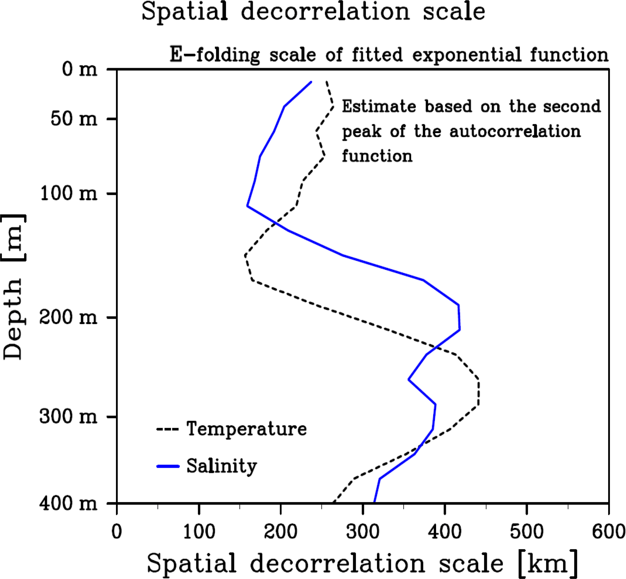
Figure C1 Vertical profile of the spatial decorrelation scales estimated from the second peak of the spatial autocorrelation function (see Fig. 10a, b). The scale is obtained from a Gaussian function fitting with two points: zero-lag autocorrelation value from Fig. 12a and the second peak. The second peak is defined by the highest autocorrelation value, the spatial lag of which is larger than 150 km. A three-layer vertical filter is applied to eliminate noise.

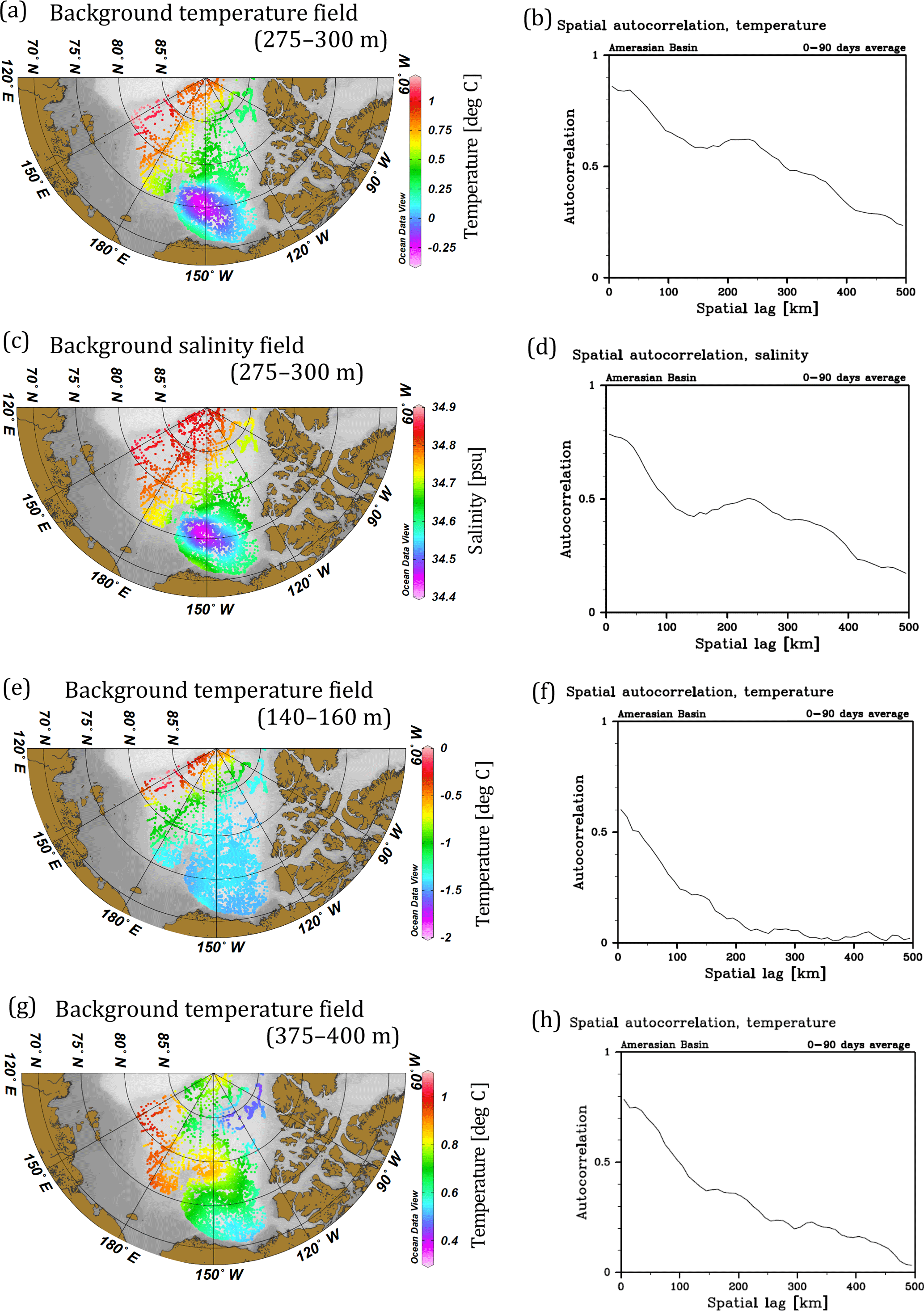
Figure C2 (a, c, e, g) Examples of the background mean fields with a circular structure associated with the Beaufort Gyre (a, c) and without the circular structure (e, g). (b, d, f, h) Spatial autocorrelation functions corresponding to their right panels. Panels (a–b) and (e–h) show temperature, while (c–d) shows salinity.

The coincidence between the second peak and the circular structure of the Beaufort Gyre indicates that the peak captures a coherent variation of isothermal (isohaline) depth. We employ level depth surfaces for the present analysis; bowl-shaped isosurfaces of T and S in the Canada Basin exhibit a circular structure on level surfaces. Due to this structure, the same isothermal (isohaline) surface appears on a level surface as it encircles the center of the Beaufort Gyre (Fig. C2a, c). The second peak captures a relatively high autocorrelation between the measurements, both of which belong to nearly the same isothermal (isohaline) surface but are separated by a certain distance in accordance with the circular pattern. A consideration of mechanisms governing the decorrelation scale further supports this interpretation. The basin-scale dynamical response of the ocean to external forcing is manifested as vertical displacements of isopycnal surfaces (with given T and S properties), resulting in coherent variations of these depth surfaces. For follow-on studies to the present one, it is desirable to calculate autocorrelation functions and decorrelation scales in a way that takes such coherent large-scale dynamic features into account. This could be achieved by analyzing anomalies of the isohaline/isothermal depth from their mean state. In the case of the Beaufort Gyre, we expect the autocorrelation functions for the variation of the isohaline/isothermal depth to have larger spatial scales than those for T and S estimated on level surfaces. As an approximate measure of the decorrelation scales for isohaline/isothermal depth anomalies, we fit a Gaussian function using the value at the zero-lag correlation and the second peak obtained from the level surface analysis (Fig. C1), resulting in roughly 200–400 km. The largest scales we find in the 200–350 m depth range for the isothermal depths and in the 150–400 m depth range for the isohaline depths correspond to the depths of strong vertical gradients of T and S. For a sound analysis, a variation of isosurface should be quantified by a variation of isosurface depth. In such an analysis, for example, salinity is no longer a variable to be examined, but depth of constant salinity surface, i.e., ${\left.Z(x,y,t)\right|}_{S=\text{constant}}$, is the variable to be examined.