Parameterization of phytoplankton spectral absorption coefficients in the Baltic Sea: general, monthly and two-component variants of approximation formulas

This paper presents approximate formulas (empirical equations) for parameterizing the coefficient of light absorption by phytoplankton a_ph(λ) in Baltic Sea surface waters. Over a thousand absorption spectra (in the 350–750 nm range), recorded during 9 years of research carried out in different months of the year and in various regions of the southern and central Baltic, were used to derive these parameterizations. The empirical material was characterized by a wide range of variability: the total chlorophyll a concentration (Tchl a) varied between 0.31 and 142 mg m⁻³, the ratio of the sum of all accessory pigment concentrations to chlorophyll a $(\sum C_i/\mathrm{Tchl}a)$ ranged between 0.21 and 1.5, and the absorption coefficients a_ph(λ) at individual light wavelengths varied over almost 3 orders of magnitude. Different versions of the parameterization formulas were derived on the basis of these data: a one-component parameterization in the “classic” form of a power function with Tchl a as the only variable and a two-component formula – the product of the power and exponential functions – with Tchl a and $\sum C_i/\mathrm{Tchl}a$ as variables. We found distinct differences between the general version of the one-component parameterization and its variants derived for individual months of the year. In contrast to the general variant of parameterization, the new two-component variant takes account of the variability of pigment composition occurring throughout the year in Baltic phytoplankton populations.

1 Introduction

If we wish to fully describe the process of photosynthesis in the seas and oceans and to correctly interpret remote observations of water bodies, it is important to obtain an accurate quantitative description of the spectral characteristics of light absorption by living phytoplankton, a significant constituent of seawater (e.g. Kirk, 1994; Mobley, 1994; Woźniak and Dera, 2007). The efficiency of sunlight absorption by this phytoplankton generally depends on a number of factors. The major, strongly absorbing components of phytoplankton cells are the pigments they contain. The principal photosynthetic pigment is chlorophyll a, which absorbs visible light mainly in two bands: one situated in the blue region, with a maximum around 440 nm, and another one in the red, with a maximum around 675 nm (e.g. Bidigare et al., 1990; Bricaud et al., 2004; Woźniak and Dera, 2007). There are also various accessory pigments, like chlorophylls b and c, carotenoids, and phycobilins. These latter pigments have different spectral absorption characteristics and may be involved in photosynthetic, photoprotective or other processes in marine organisms. The pigment composition of photosynthesizing marine species can differ, since it can in a general sense reflect the adaptation of an organism to different light conditions (photo- and chromatic adaptation) as well as acclimation at the plant community level (e.g. Kirk, 1994; Woźniak and Dera, 2007). Overall, analysis of pigment composition data obtained for marine phytoplankton assemblages from various ocean and sea waters has revealed a general trend indicating that the proportion of accessory pigments relative to chlorophyll a decreases with increasing chlorophyll a concentration (increasing trophicity) (e.g. Woźniak and Ostrowska, 1990a; Trees et al., 2000; Babin et al., 2003). Even so, there is substantial variability around this trend. Hence, the main factor that light absorption by phytoplankton assemblages depends on is the pigment composition. Another important factor, where absorption by phytoplankton is concerned, is how densely the strongly light-absorbing pigments are “packed” within the internal structures of individual cells (the so-called “packaging effect”; Morel and Bricaud, 1981, 1986). Increasing intracellular pigment concentrations and cell size flatten the real absorption spectra compared to what one may expect from a simple addition of the absorption coefficients of individual pigments.

Given the complexity of all these relationships, it is often necessary (or even required) for practical purposes to take a highly simplified approach, for example, when constructing models of bio-optical processes for interpreting remote sea observations. It is a common simplification to assume that all the relevant properties of a phytoplankton population can be roughly parameterized with the aid of just one variable – the concentration of chlorophyll a: indeed, the total biomass of an entire phytoplankton population as well as its diverse optical properties are often parameterized in this way. Earlier authors addressing this question applied this kind of simplification in attempts to determine typical values of the “chlorophyll a specific” absorption coefficient (defined as the light absorption coefficient of phytoplankton normalized to the chlorophyll a concentration). In practice, therefore, the adoption of one averaged value of this coefficient should enable the relationship between the phytoplankton absorption coefficient and the chlorophyll a concentration in seawater to be described using the simplest possible, i.e. linear, functional relationship. As measured in nature, however, values of the specific absorption coefficient have proved to be highly variable. The papers by Bricaud et al. (1995, 1998), often cited by other authors, were among the first to introduce for practical purposes a different, non-linear, approximate description of the light absorption vs. chlorophyll a concentration relationship. They proposed using a power function to account for the general decrease in light absorption efficiency per unit chlorophyll a concentration that occurs with increasing absolute values of this concentration in seawater (the relevant mathematical formulas are given later in the text). Bricaud et al. (1995) also gave a theoretical explanation of these effects, suggesting that there might be a correlation between the increase in the absolute chlorophyll a concentration and the increasing contribution of the pigment packaging effect and, concurrently, the decreasing proportion of pigments other than chlorophyll a. The papers by Bricaud et al. (1995, 1998) were based on extensive empirical material gathered in different regions of open, oceanic waters, classified as “Case 1” waters. Different authors addressed the same problem in many later papers: examples of spectral power function parameterizations for different marine environments can be found in, for example, Stramska et al. (2003), Staehr and Markager (2004), Matsuoka et al. (2007), Dmitriev et al. (2009), Nima et al. (2016), Churilova et al. (2017), and Mascarenhas et al. (2018). The subject literature also provides examples of similar parameterizations derived for inland water bodies, for example by Reinart et al. (2004), Ficek et al. (2012a, b), Ylöstalo et al. (2014) and Paavel et al. (2016). All of these papers give spectral coefficients of parameterizations tailored to specific datasets differing from each other to a greater or lesser extent. Obviously, all such parameterizations are far-reaching simplifications of the complex dependences observed in nature. That there might be significant deviations from the approximate “average” relationship was already made clear by Bricaud et al. (1995) in their original work; these authors subsequently analysed the potential causes of this differentiation (Bricaud et al., 2004). Using indirectly reconstructed information regarding the size structure of the ocean phytoplankton population, they were able to estimate separately the impacts of the differences in the dominant sizes of plankton populations and the differences in pigment composition on the relationship in question. In general, they found that for oligo- and mesotrophic waters (i.e. waters with chlorophyll a concentrations < 2 mg m⁻³), the variability associated with the packaging effect might be exerting a more significant influence, whereas in eutrophic waters (with higher chlorophyll a concentrations) both effects might be of equal weight. Generally, however, the observed variability indicates that one should expect both regionally and seasonally differentiated forms of such simplified relationships to occur instead of one universal, approximate statistical relationship between a_ph(λ) and the chlorophyll a concentration.

The Baltic Sea, the region we have been studying, is a semi-enclosed, brackish water basin classified as an example of “Case 2” waters. It is characterized by usually high concentrations of terrigenous dissolved organic substances (e.g. Kowalczuk, 1999; Meler et al., 2016a). The biomass and species composition of living phytoplankton in the Baltic is known to vary during the year. Usually there are three main phytoplankton blooms: a spring bloom of cryophilous diatoms, which transforms into a bloom of dinoflagellates (early March–May); a summer bloom of cyanobacteria (July and August); and an autumn bloom of thermophilous diatoms (September–October) (Wasmund et al., 1996, 2001; Witek and Pliński, 1998; Wasmund and Uhlig, 2003; Thamm et al., 2004).

In an earlier paper by our research team (Meler et al., 2017a), we provided an initial version of the power function parameterization, adjusted to data collected in the southern Baltic Sea. However, these preliminary analyses, focusing mainly on pooled data from marine and lacustrine environments, were based on a much smaller set of data than the one we currently have, and the initial parameterization was carried out for all the data pooled, regardless of when they were acquired. On the other hand, another recent paper of ours identified significant differences in the absorption properties of Baltic phytoplankton at different times of the year (Meler et al., 2016b). In a further preliminary study, limited to just the single light wavelength of 440 nm, we demonstrated differences between the coefficients of the relevant simplified parameterizations when they were tailored to data gathered at specific times of the year (Meler et al., 2017b). It is in this context, therefore, that we have decided in the present paper to readdress the problem of determining practical forms of a simplified parameterization of the phytoplankton absorption coefficient appropriate to Baltic Sea conditions.

The objectives of this work are twofold.

• The main one is to find new forms of the classic, one-component power function parameterization for the phytoplankton absorption coefficient adapted to the specific conditions of the Baltic Sea. An important aspect of this is to record the extent of the differences between the coefficients of spectral parameterization when they are derived separately for data from selected periods of the year. These new analyses, as opposed to the preliminary results published earlier, have to be performed over a wide spectral range, with a sufficiently high resolution, on the currently available extended dataset and also in accordance with the latest recommended calculation procedures.

• An additional aim of this work is to propose a modified but still relatively simple, new form of parameterization enabling the diversity of phytoplankton absorption properties observed in the study area during the year to be taken into account. The new forms of parameterization that we are seeking can be used, among other things, to develop and improve the accuracy of practical, local algorithms for interpreting remote observations of the Baltic Sea.

2 Materials and methods

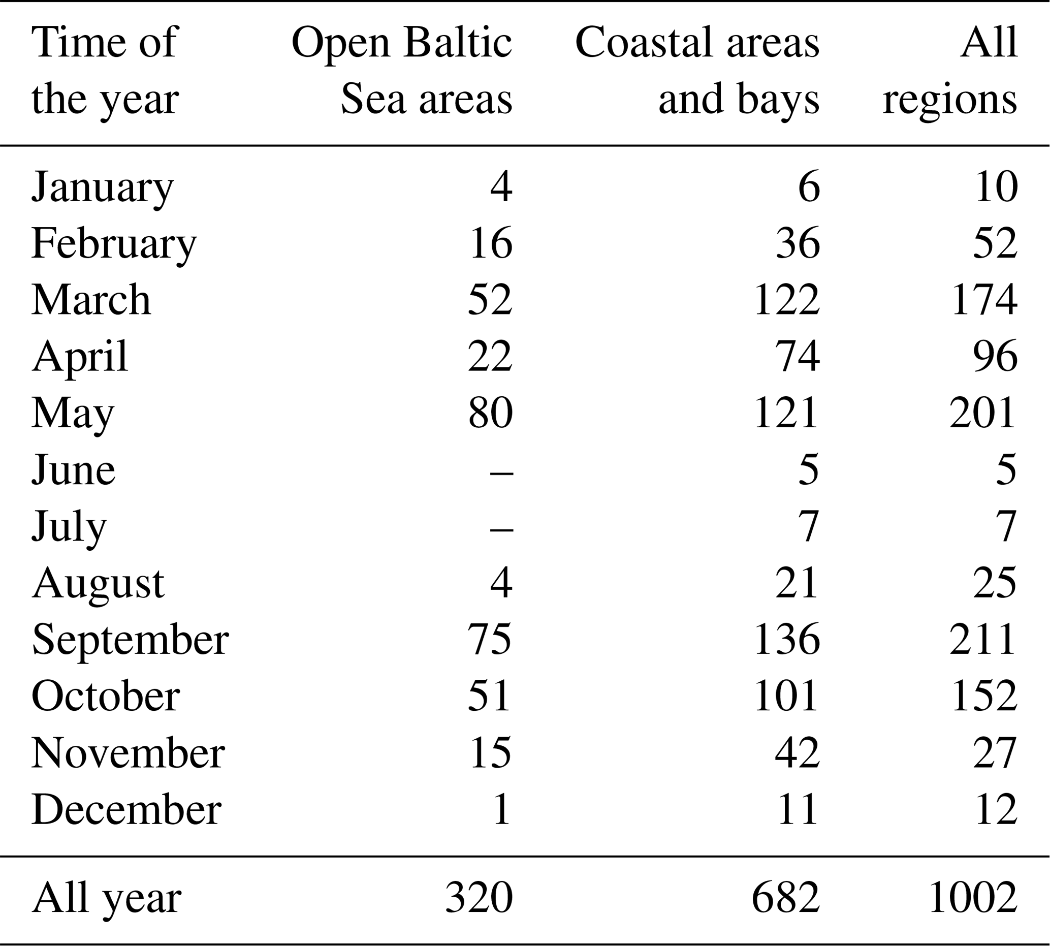
The empirical data used in this study were collected at more than 170 measuring stations in various parts of the southern and central Baltic Sea, though mainly in the Polish economic zone, from 2006 to 2014 (Fig. 1). These data were acquired principally during 42 short research cruises on board R/V Oceania at different times of the year, but mostly from March to May and from September to October (about 80 % of the data analysed in this paper are from these periods). The practice during each cruise was to select measuring stations that were maximally diverse with respect to their optical properties, i.e. in the vicinity of river mouths and estuaries (the rivers Vistula, Oder, Reda, Łeba and Świna; the Szczecin Lagoon), bays and offshore waters (Gulf of Gdańsk, Puck Bay and Pomeranian Bay), and open southern Baltic waters. During three cruises (in May of 2010, 2012 and 2014), measurements were also made in the open waters of the central Baltic. However, because of weather- and sea-state-related limitations, only 32 % of the data are from open-water regions (Table 1). In addition to the cruise measurements, data were gathered throughout the year by sampling the seawater at the end of the ca. 400 m long pier in Sopot, on the Gulf of Gdańsk coast (< 7 % of the overall number of data analysed).

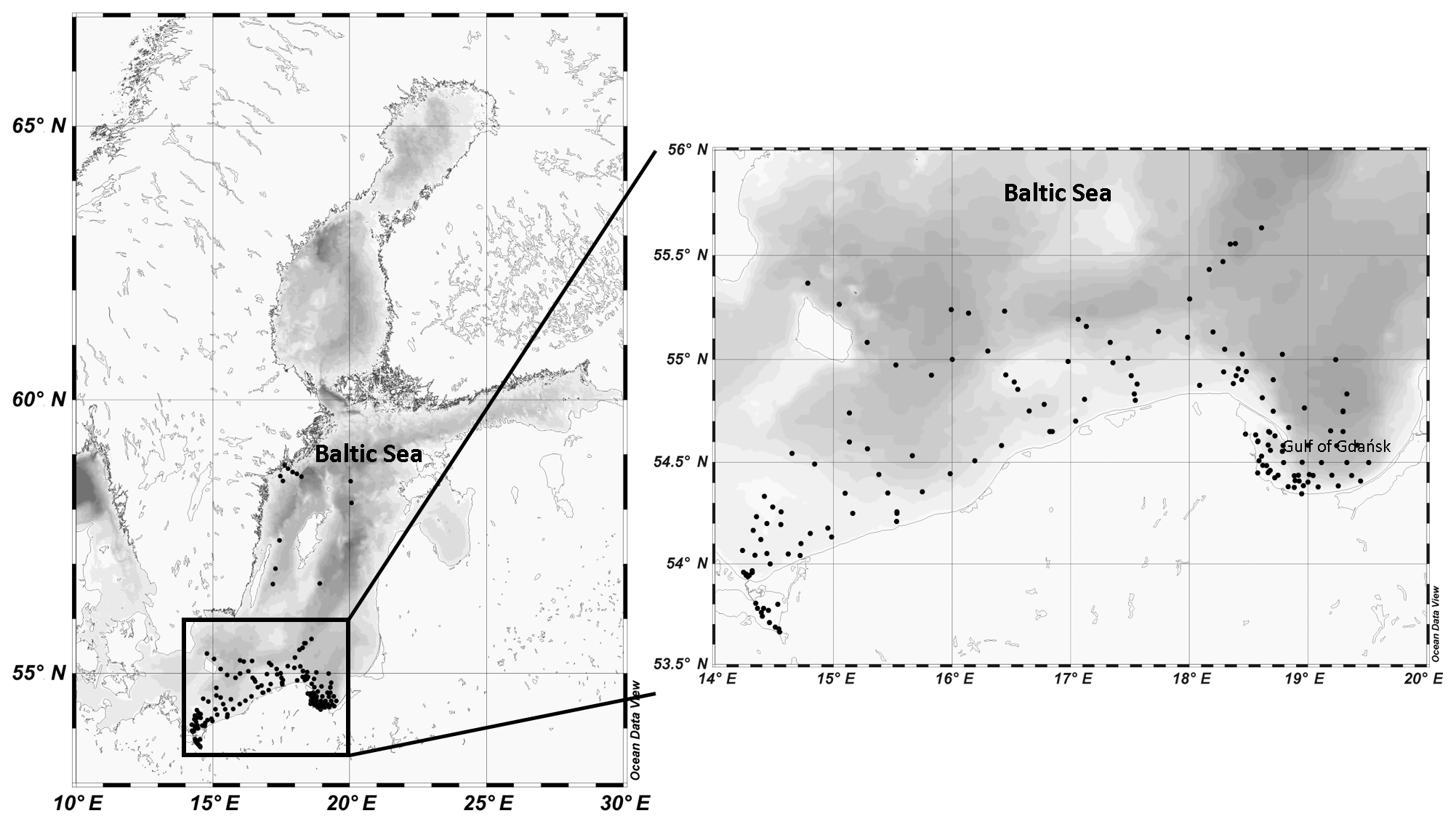
Figure 1 Locations of all the sampling stations in the Baltic Sea; enlarged view of the study area.

Table 1 Numbers of seawater samples analysed, divided into the months and areas of their acquisition.

During the research cruises, a diversity of physical and optical parameters of seawater were measured in situ at each sampling station, and discrete seawater samples were collected for further laboratory analysis of certain optical properties (spectra of coefficients of light absorption by phytoplankton) and biogeochemical properties (concentrations of chlorophyll a and other phytoplankton pigments). These samples were collected with a Niskin bottle (height ca. 0.9 m, capacity 25 L) immersed just below the surface; in shallow estuarine areas and river mouths (sampled from a pontoon) or off the end of the Sopot pier, they were obtained with a bucket. Immediately after collection, all samples were passed through glass fibre filters (Whatman, GF/F, 25 mm, nominal retention of particles with sizes down to 0.7 µm) at a pressure not exceeding 0.4 atm. The volumes filtered were chosen on a case-by-case basis; between 2 and 1150 mL of seawater were filtered for later absorption measurements, and generally between 150 and 1000 mL were filtered for phytoplankton pigment concentration analysis. All sample filters were immersed in a Dewar flask containing liquid nitrogen (at about −196 ^∘C) and then kept frozen (at about −80 ^∘C) for further analysis in the laboratory on land.

In order to determine the spectra of the phytoplankton absorption coefficient a_ph, we measured the absorption coefficient spectra for all suspended particles retained on filters (a_p) and also, after chemical bleaching of the pigments in our samples, the corresponding spectra of non-algal particles (a_NAP). We performed the optical measurements in the 350–750 nm spectral range with a UNICAM UV4-100 double-beam spectrophotometer equipped with an integrating sphere with an external diameter of 66 mm (LABSPHERE RSA-UC-40). For the reference measurements we used clean filters rinsed with particle-free seawater. The methodology of combined light-transmission and light-reflection measurements (known as the T–R method) was that described by Tassan and Ferrari (1995, 2002). From the pooled results of these measurements (several scans in different configurations), we calculated the optical density OD_s(λ) representing each filtered sample. As opposed to standard spectrophotometric analyses performed in transmission mode only, at least in theory, the results of T–R method should not need to be corrected for the so-called “scattering error”. But in order to calculate absorption coefficients of particles in solution, an additional correction has to be made to compensate for the elongation of the optical path of the light owing to the multiple scattering occurring in the filtered material. This is done by applying the dimensionless path length amplification, the β factor, which converts the measured optical density of particles collected on the filter (OD_s(λ)) into the optical density characterizing these particles in solution (OD_sus(λ)) (Mitchell, 1990). In our analyses we used the new β-factor formula proposed by Stramski et al. (2015) for the T–R method:

$$\begin{array}{}\text{(1)}& {\mathrm{OD}}_{\mathrm{sus}}\left(\mathit{\lambda }\right)=\mathrm{0.719}{\mathrm{OD}}_s(\mathit{\lambda }{)}^{\mathrm{1.2287}}.\end{array}$$

The coefficient of light absorption by all suspended particles was then calculated using the formula

$$\begin{array}{}\text{(2)}& a_{\mathrm{p}}\left(\mathit{\lambda }\right)=\left[\ln \right(\mathrm{10})\cdot {\mathrm{OD}}_{\mathrm{sus}}(\mathit{\lambda }\left)\right]/l,\end{array}$$

where l (m) is the hypothetical optical path in solution, determined as the ratio of the volume of filtered water to the effective area of the filter. The absorption by non-algal particles a_NAP(λ) was determined in an analogous way, after the phytoplankton pigments had been bleached for 2–3 min with a 2 % solution of calcium hypochlorite Ca(ClO)₂ (Koblentz-Mishke et al., 1995; Woźniak et al., 1999); thereafter, the sample filter was rinsed with a small volume of particle-free seawater to remove any bleach residue, as this could additionally absorb light at short wavelengths. Finally the sought-after coefficient a_ph was calculated as the difference between a_p and a_NAP.

In practice, however, we had to add two corrective procedures to the protocols described above. One related to the noise which appeared in the individual spectra recorded with our spectrophotometer. To partially eliminate it, we applied a “spectral smoothing” procedure – the spectral five-point “moving average” was repeated 3 times – to the calculated individual spectra of both coefficients a_p and a_NAP. This procedure partially eliminated fluctuations of the signal between adjacent light wavelengths but did not significantly affect the magnitude of the major absorption peaks, the “half-widths” of which are of the order of tens of nanometres. The other corrective procedure related to the small deviations from zero of the calculated coefficients a_ph at wavelengths close to 750 nm. It is generally assumed that the light absorption of phytoplankton pigments in this spectral range should be negligible (Babin and Stramski, 2002). The occurrence of non-zero values in this range may be due to several different factors: differences in the optical properties of individual glass fibre filters, the difficulty of maintaining ideally repeatable filter moisture during measurements and the possible partial loss of sample material as a result of the filters being rinsed after bleaching. To correct for all these effects we applied a simple “null-point” correction (e.g. Mitchell et al., 2002). The average coefficient a_ph calculated in the range between 740 and 750 nm was subtracted from the values of a_ph across the entire spectrum. Generally different factors may have influenced the final uncertainty of our absorption measurements. Among them is the instrument noise present in each individual spectrophotometric scan (in each configuration) and also the possible uncertainty in path length amplification factor, volume filtered and filter area used in subsequent calculations, as well as uncertainty coming from subsampling from larger volumes of water. As a strict estimation of all these inaccuracies would be very complicated (due to the mathematical complexity of the algorithm used according to Tassan and Ferrari, 1995, 2002), here we limit ourselves only to estimating some of these inaccuracies. The mean inaccuracy caused by instrument noise occurring in separate measurements of light absorption by particles before and after bleaching we estimated to be $\mathrm{\Delta }{a}_{\mathrm{ph}}=\mathrm{5.68}\times {\mathrm{10}}^{-\mathrm{3}}$ m⁻¹ ($\pm \mathrm{9.13}\times {\mathrm{10}}^{-\mathrm{3}}$ m⁻¹, standard deviation (SD)). We assumed that the uncertainty of a_ph (Δa_ph) can be calculated as a square root of a sum of squares of uncertainties Δa_p and Δa_NAP. The latter were estimated as 95 % prediction intervals (=1.96 SD) for a_p and a_NAP values between 740 and 750 nm, where it is assumed that the absorption signal should be flat. Dividing the mean value of Δa_ph by corresponding measured values of a_ph(440) or a_ph(675) gave percentage error distributions with mean values of 2.3 % and 5.9 %, respectively (with SD of 2.3 % and 7.6 %, respectively). In the collected dataset, due to logistic limitations, generally no measurements were made on multiple samples. However, in the separate tests we estimated the average uncertainty of a_ph measurements due to subsampling to be 9.1 % (±1.5 %, SD).

High performance liquid chromatography (HPLC) was used to determine phytoplankton pigment concentrations; the methodology is described in detail in Meler et al. (2017b), Stoń and Kosakowska (2002), and Stoń-Egiert and Kosakowska (2005). In this work we refer mainly to the total chlorophyll a concentration (Tchl a) (defined as the sum of chlorophyll a, allomer and epimer, chlorophyllide a, and phaeophytin a) and to the sum of the concentrations of all accessory pigments ΣC_i, i.e. the sum of chlorophylls b (Tchl b), chlorophylls c (Tchl c), photosynthetic carotenoids (PSC) and photoprotective carotenoids (PPC). The precision of HPLC measurements was estimated as equal to 2.9 % (±1.5 %, SD) and an error related to subsampling as 9.7 % (±6.4 %, SD) (Stoń-Egiert et al., 2010).

The data were analysed statistically in order to characterize their variability and to find approximate empirical relationships between them. The variability of the target optical and biogeochemical quantities ranged over almost 3 orders of magnitude. Therefore, to assess the uncertainty of our empirical parameterizations, we applied standard arithmetic statistics of relative error and also separate statistics of logarithmically transformed data (so-called logarithmic statistics). The exact formulas are given as a footnote to Table 3 later in the paper.

3 Results and discussion

3.1 General characteristics of the data

Figure 2 exemplifies selected spectra of a_ph that we recorded in the Baltic Sea. Even though they were smoothed using the previously described raw data procedure, some still contain artefacts related to the noise occurring in our measurement system. These artefacts are particularly visible in the 350–400 nm range, where the accuracy of measurements is limited owing to the strong light attenuation by the glass fibre from which the filters are made, and also in the 550–650 nm range, where the absorption signal is small compared to other bands. In spite of these imperfections, 80 % of these spectra exhibit the expected characteristic absorption maxima in both the blue (ca. 440 nm) and red (ca. 675 nm) bands. Some of the spectra in our set, however, do not show a significant increase in light absorption with increasing wavelength in the 350–440 nm range: in 20 % of the spectra recorded a_ph(400)∕a_ph(440) is > 0.95 (in some cases as high as 1.42), mainly for samples from near the mouth of the River Vistula, in the Szczecin Lagoon and off the Sopot pier. The first part of Table 2 lists basic statistical information characterizing the ranges of variation in the light absorption coefficient at selected light wavelengths. In fact, the variability of a_ph(λ) over the entire spectral range examined, calculated for individual light wavelengths, was almost 3 orders of magnitude. For blue light, for example, a_ph(440) varied from 0.014 to 3.85 m⁻¹, whereas for the local absorption maximum in the red band, a_ph(675) varied from 0.006 to 1.74 m⁻¹.

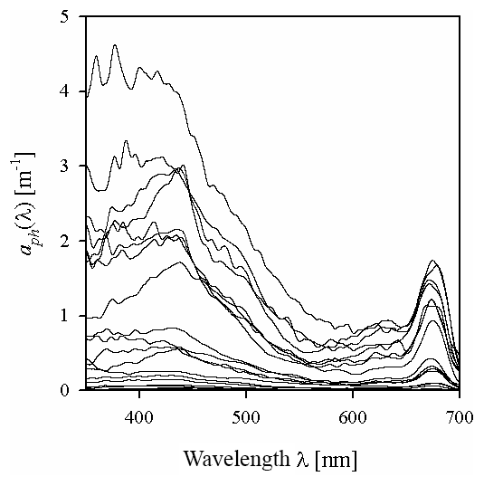
Figure 2 Examples of the spectra of the light absorption coefficient a_ph(λ) representing the variability range of the data analysed in the present paper.

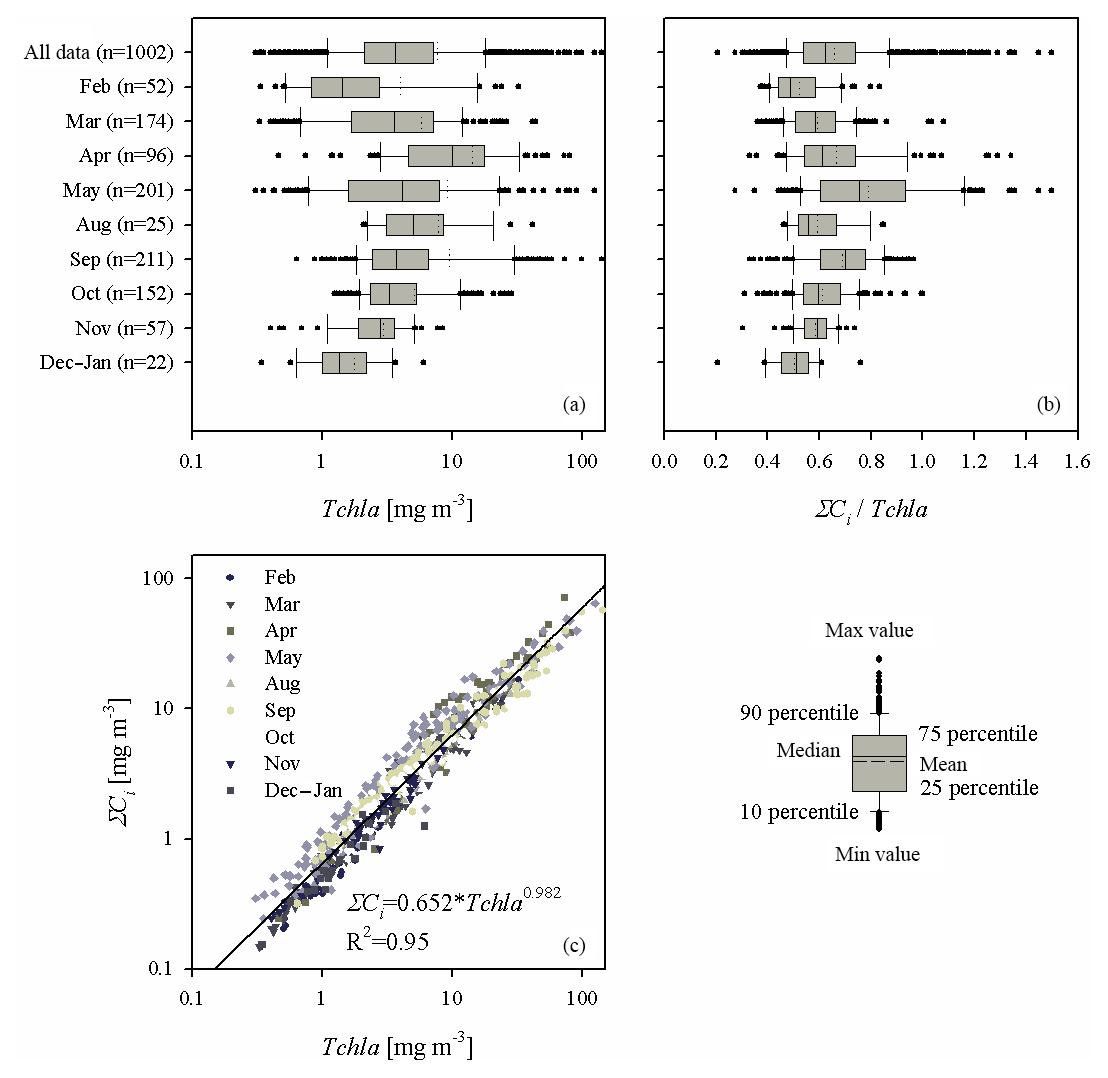
Figure 3 (a) Box plot presenting the range of variation in chlorophyll a concentration (Tchl a) for all the data analysed and for each sampling month; (b) as (a) but showing the ratio of the sum of accessory pigments to the chlorophyll a concentration (ΣC_i∕Tchl a); (c) graph illustrating the relationship between ΣC_i and Tchl a – the solid line represents a simple functional approximation of the relationship (the equation is given in the panel).

Table 2 Variability ranges of selected optical and biochemical quantities characterizing phytoplankton in samples from the Baltic Sea.

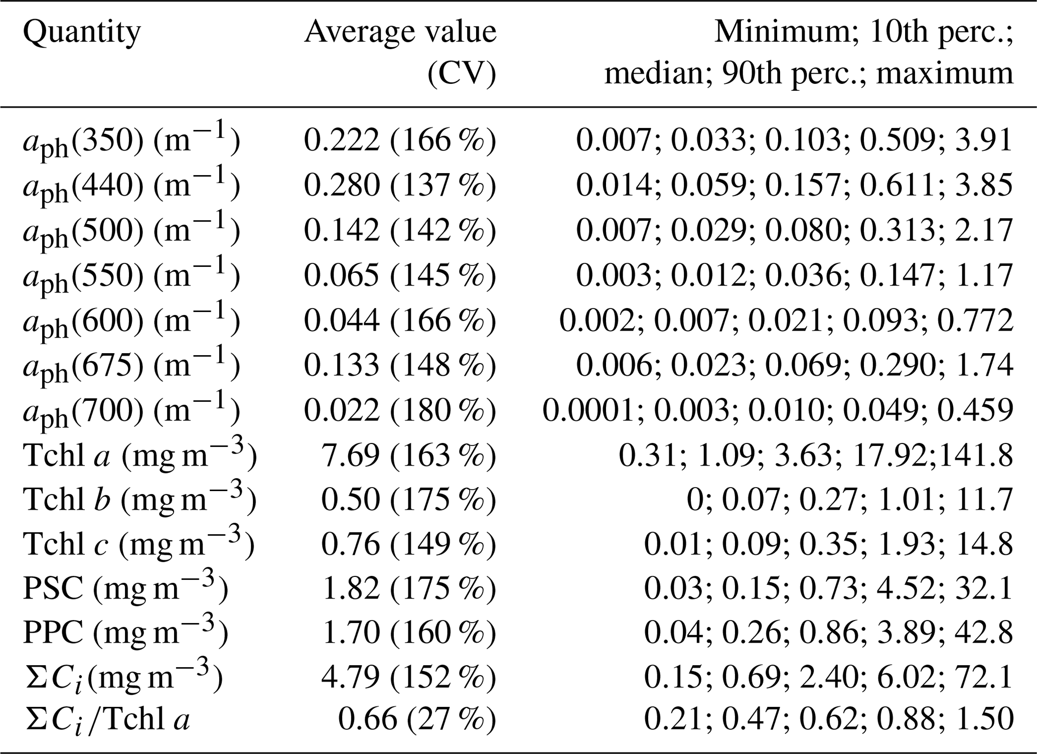
The second part of Table 2 provides statistical information illustrating the variability in concentration of the basic photosynthetic pigment chlorophyll a (Tchl a) and also the concentrations of different groups of accessory pigments, i.e. chlorophylls b and c, and other photosynthetic and photoprotective pigments (Tchl b, Tchl c, PSC and PPC). In addition, the table lists the total concentration of all accessory pigments (ΣC_i) and the ΣC_i∕Tchl a ratio. Figure 3 illustrates the variabilities of Tchl a and ΣC_i as well as their ratio for all the pooled data, broken down into individual sampling periods (months). This shows that with respect to all the data analysed, the ranges of variability of both Tchl a and ΣC_i are, like the absorption coefficient, almost 3 orders of magnitude (0.41–141.8 and 0.15–72.1 mg m⁻³, respectively). The average Tchl a for all the data was 7.69 mg m⁻³. In the spring and summer months when we were able to make measurements at sea, mean values of Tchl a were above average, while in autumn and winter they were lower. In general, a similar trend of average changes in individual months emerges from an analysis of the sum of accessory pigment concentrations ΣC_i. Taking into account all the data from different periods of the year, we can say that measured values of ΣC_i correlate fairly well with Tchl a (the approximate equation and the coefficient of determination R² are given in Fig. 3c). Nevertheless, if we look at the ΣC_i∕Tchl a ratio, we see that its average values also changed significantly during the year (Fig. 3b). The average ΣC_i∕Tchl a for all the data was 0.66, but the full range of variability that we recorded was from 0.21 to 1.5. For the months of April, May and September, the average ΣC_i∕Tchl a was higher than or equal to the average for the whole year (0.66, 0.79 and 0.69, respectively). In the remaining months, the averages were lower than the general average – from 0.50 to 0.61. This latter fact is a clear indicator of the obvious limitations of applying solely the chlorophyll a concentration as a simplified measure to describe the overall pigment population and to which measure the light absorption of pigments is customarily parameterized.

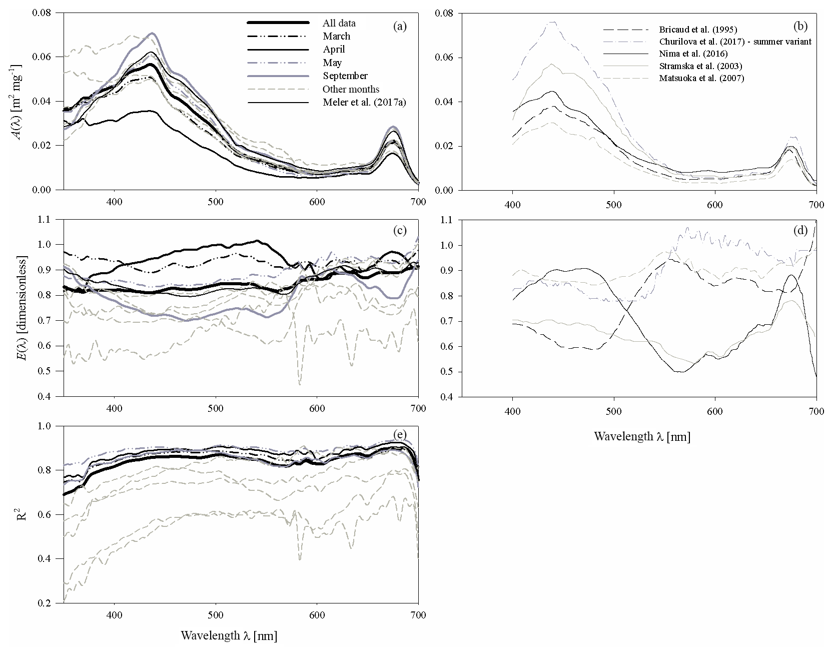
Figure 4 (a, c) Spectral plots of coefficients A and E of the parameterizations described by Eq. (3a), and (e) the corresponding values of coefficient R², determined for all the data analysed and for each sampling month. The coefficients of the preliminary parameterization given in Meler et al. (2017a) are also plotted; (b, d) examples of coefficients A and E given by various authors (the legend is given in b).

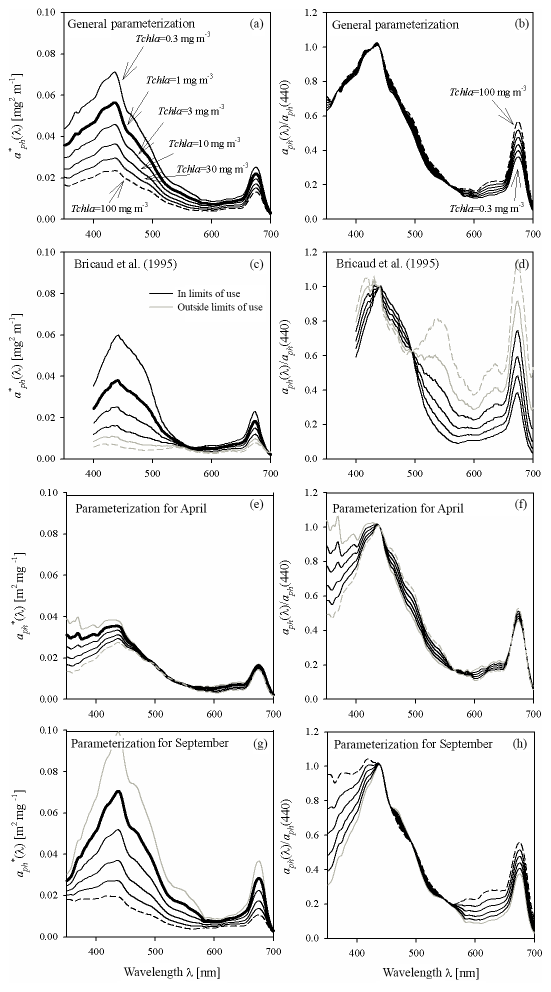
Figure 5 Example spectra of the specific coefficients of light absorption by phytoplankton $a_{\mathrm{ph}}^{\ast }\left(\mathit{\lambda }\right)$ (left-hand column) and spectra of a_ph normalized to its own value in the 440 nm band (right-hand column) for some values of Tchl a between 0.3 and 100 mg m⁻³: (a, b) estimated using the general variant of the parameterization obtained in this paper; (c, d) estimated on the basis of the parameterization by Bricaud et al. (1995) (the grey lines in c and d represent chlorophyll a concentrations Tchl a that go beyond the range for which the Bricaud et al. parameterization was originally developed); (e, f) estimated using the variant of parameterization obtained in this paper for April data only; (g, h) estimated using the variant for September data only.

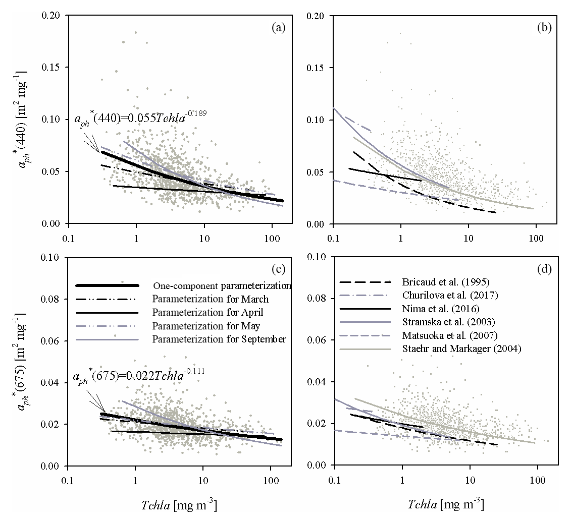
Figure 6 (a) Relationship between coefficient $a_{\mathrm{ph}}^{\ast }$(440) and the chlorophyll a concentration Tchl a and its functional approximations determined in this study for all the data analysed and for selected sampling months (the legend is given in c; the equation given in the panel represents approximations of all the data available; for coefficients obtained for particular months, see Table A2 in Appendix A); (c) as in (a) but for $a_{\mathrm{ph}}^{\ast }$(675); (b, d) plots similar to (a, c) but presenting examples of functional approximations determined by various authors (the legend is given in d). The grey dots in each panel represent individual data points from our database.

3.2 Approximate description of the light absorption coefficient by phytoplankton

3.2.1 General and monthly variants of one-component parameterizations

We carried out statistical analyses of our measurement data in order to define classic forms of the approximate functional relations between the light absorption coefficient a_ph(λ) and the concentration Tchl a. Like Bricaud et al. (1995, 1998), we approximated these relations using power functions. With linear regression applied to the logarithms of the input data for each light wavelength (regression between log(a_ph(λ)) and log(Tchl a)), the coefficients A and E of the following approximated parameterization could be calculated:

$$\begin{array}{}\text{(3a)}& a_{\mathrm{ph}}\left(\mathit{\lambda }\right)=A\left(\mathit{\lambda }\right)\cdot \mathrm{Tchl}{a}^{E\left(\mathit{\lambda }\right)}.\end{array}$$

Note that coefficient A(λ) determined in this way reflects the numerical value of the light absorption coefficient a_ph(λ) that the approximated relationship assigns to the case when the Tchl a is exactly 1 mg m⁻³. The coefficient E(λ) of Eq. (3a) is a dimensionless quantity, which is the exponent of the power to which the chlorophyll a concentration is raised. If its value is < 1, there is a statistical tendency for the phytoplankton absorption efficiency to decrease per unit mass of chlorophyll a with increasing absolute chlorophyll a concentration. A value of E=1 would mean a stable a_ph to Tchl a ratio, while a value of E > 1 would imply a statistical tendency for a_ph∕Tchl a to increase with increasing Tchl a. By performing linear regression of the logarithms of the input data, we were also able to calculate the determination coefficients R² for the approximated parameterization at the individual wavelengths of light. The parameterization coefficients A and E given by Eq. (3a) can be easily used to determine the specific coefficient of light absorption by phytoplankton $a_{\mathrm{ph}}^{\ast }\left(\mathit{\lambda }\right)$ (m² mg⁻¹) (defined as values of a_ph(λ) normalized with respect to Tchl a):

$$\begin{array}{}\text{(3b)}& a_{\mathrm{ph}}^{\ast }\left(\mathit{\lambda }\right)=A\left(\mathit{\lambda }\right)\cdot \mathrm{Tchl}{a}^{E\left(\mathit{\lambda }\right)-\mathrm{1}}.\end{array}$$

The coefficients of the approximate Eq. (3a) were determined over the entire available spectral range from 350 to 700 nm with a resolution of 1 nm. Figure 4a, c and e present different variants of the spectra of coefficients A(λ) and E(λ), along with the respective values of R². These variants represent parameterizations based on all available data (a general variant) as well as alternative parameterizations derived for data subsets relating to particular months (monthly variants). The parameterization coefficients for the general and selected monthly variants are listed in the Appendix A (Tables A1 and A2). Analysis of the curves in Fig. 4a and c shows that the coefficients of the monthly parameterizations differ, exhibiting larger or smaller deviations from the course of the general variant's coefficients. In the case of coefficient A, the differences between 350 and 590 nm and around 675 nm are particularly conspicuous. For example, the highest values of coefficient A for the 440 nm band were obtained in the case of parameterizations derived for September and December–January and the lowest for April. With regard to the spectral slope of coefficient A in the 350–440 nm range, the largest deviations from the typical course were recorded for December–January, April, and February. In contrast, the parameterizations obtained for March, May and October are the closest to the general variant with respect to A. As regards coefficient E, there are differences between the alternative parameterizations over the entire spectral range. In the general variant, E changes only slightly, between 0.81 and 0.91. On the other hand, the values of E for the parameterizations derived for individual months are spectrally more differentiated, with more pronounced local maxima and minima. The deviations from the general case of the parameterizations are the largest for March and April (upward) and for December–January (downward). The determination coefficients R², which may initially characterize the accuracy of the absorption coefficient parameterization using Eq. (3a), are relatively high in the case of the general variant of parameterization, i.e. no less than 0.8, over almost the entire visible light range. Lower values of R² are found only at the edges of the spectral range examined, where either the accuracy of measurements is expected to be lower (short wavelengths) or the values of the absorption coefficient are close to zero (long wavelengths). In the case of the monthly parameterizations, only the formulas obtained for months with relatively large amounts of data take equally high values of R² (i.e. March, April, May and September). For the other months, values of R² are < 0.8, at least in significant parts of the spectral range examined.

Figure 7 (a) Spectral plots of coefficients A₀ and Kof the two-component parameterization described by Eq. (4); (b) examples of curves representing coefficent A^′(λ, ΣC_i∕Tchl a), defined by Eq. (5), for the following values of ΣC_i∕Tchl a: the average value of 0.62; selected values between 0.39 and 1.15 (representing the range from the 10th percentile for the December–January period to the 90th percentile for May); the hypothetical value of 0.

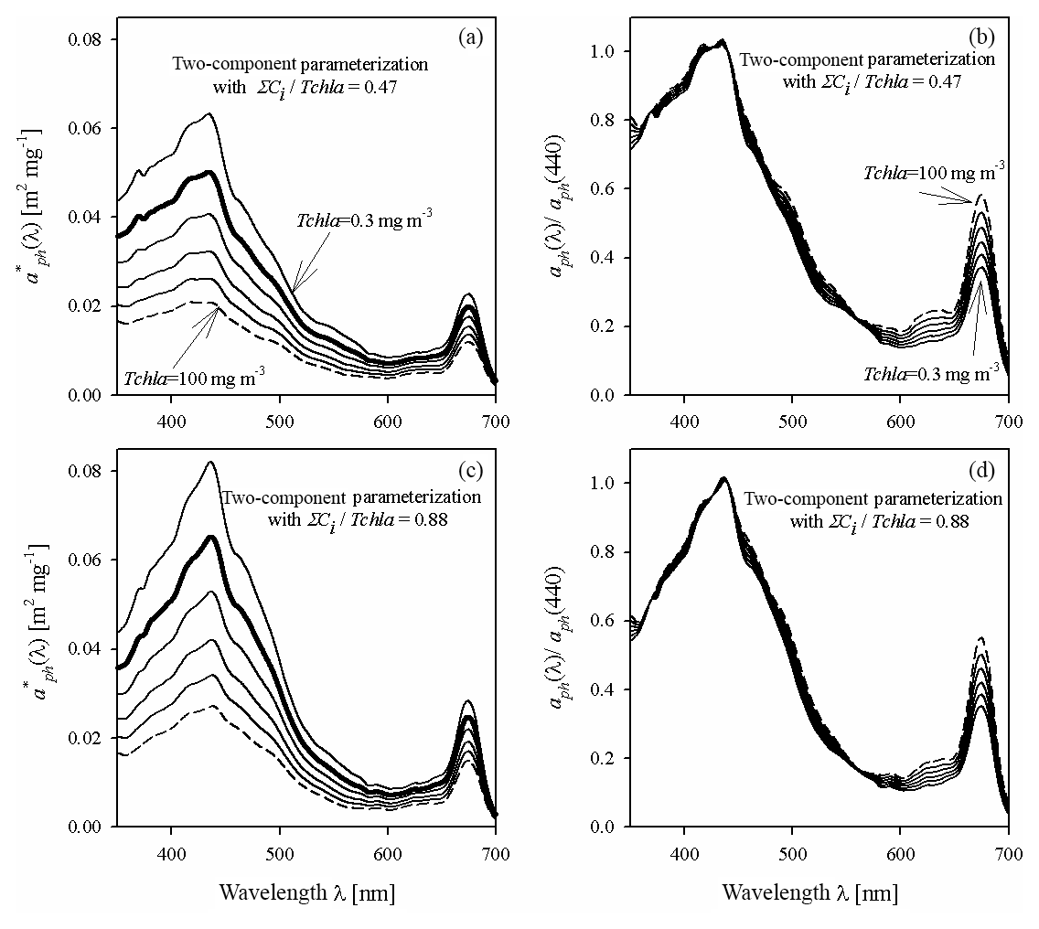
Figure 8 Example spectra of the specific coefficient of light absorption by phytoplankton $a_{\mathrm{ph}}^{\ast }$ (a, c) and spectra of coefficient a_ph normalized to its value in the 440 nm band (b, d), for some values of Tchl a between 0.3 and 100 mg m⁻³, estimated by the two-component parameterization Eq. (4), and for two different assumed constant values of the pigment concentration ratio ΣC_i∕Tchl a: 0.47 (representing the 10th percentile for all data) and 0.88 (representing the 90th percentile for all data).

Figure 5 illustrates important aspects of the variability in magnitude and spectral shape of the absorption coefficient when certain variants of the parameterization are used to calculate it. Figure 5a illustrates the family of curves representing the specific coefficients of light absorption by phytoplankton $a_{\mathrm{ph}}^{\ast }\left(\mathit{\lambda }\right)$ calculated according to the general variant of our new parameterization. These curves are plotted for a few chlorophyll a concentrations from the 0.3–100 mg m⁻³ range (corresponding more or less to the range that we recorded in the Baltic Sea). The bold line in Fig. 5a outlines the spectrum calculated for Tchl a = 1 mg m⁻³ (corresponding to the numerical value of coefficient A(λ)). In addition, to better visualize the “evolution” of the spectral shape of the predicted spectra of a_ph, another family of curves is plotted. The spectra of a_ph, normalized with respect to 440 nm, are plotted in Fig. 5b and f for values of Tchl a from the same range. To provide some background, Fig. 5c and d show two analogous diagrams obtained using the “classic” parameterization developed by Bricaud et al. (1995) (although it should be mentioned that the two highest Tchl a values – 30 and 100 mg m⁻³ – generally lie beyond the range for which Bricaud et al. (1995) originally developed their parameterization). Both parameterizations, our new one and the classic one according to Bricaud et al. (1995), clearly predict drops in $a_{\mathrm{ph}}^{\ast }\left(\mathit{\lambda }\right)$ with increasing Tchl a. But where changes in spectral shapes are concerned, our general parameterization predicts significant changes only in the 600–680 nm spectral range, whereas according to Bricaud et al. (1995) the variations should occur over a much broader spectral range (Fig. 5b and d). Both parameterizations qualitatively predict the well-known phenomenon of absorption spectra “flattening” with increasing Tchl a (e.g. Morel and Bricaud, 1981), but these predictions are quantitatively different. As a simplified measure of spectra flattening, one can analyse, for example, the changes in the ratio of a_ph(440) to a_ph(675): this ratio is sometimes referred to as the “colour” or “pigment” index (e.g. Woźniak and Ostrowska, 1990a and b; see also Bricaud et al. 1995). When the parameterization by Bricaud et al. (1995) is applied to the range of Tchl a changes assumed here (from 0.3 to 100 mg m⁻³), the colour index decreases roughly threefold, i.e. it decreases from 2.69 to 0.88, the latter value signifying a greater absorption of light in the red band than in the blue. By contrast, with our new parameterization, the colour index drops by a factor of only around 1.57 (from 2.76 to 1.76). These differences indicate that the combined influence of the packaging effect and the decrease in relative accessory pigment concentrations manifests itself differently in our Baltic Sea dataset than in the original oceanic dataset of Bricaud et al. (1995). Besides these differences, however, we would also like to point out clear differences that become apparent when different parameterizations matched to individual months are applied to our dataset. Fig. 5e, f, g and h show similar spectral curves for two contrasting months: April and September. The family of $a_{\mathrm{ph}}^{\ast }\left(\mathit{\lambda }\right)$ curves plotted for April (Fig. 5e) shows generally much lower values in the blue light maximum and less steep slopes around this maximum than the corresponding curves for September (Fig. 5g). Also, the variability in the normalized shapes of coefficient a_ph is greater and more complex for these two particular months (Fig. 5f to h) than was the case with the general parameterization (Fig. 5b). The colour index changes only by a factor of 1.16 (a drop from 2.2 to 1.9) for April, while for September the corresponding change is by a factor of 1.49 (a drop from 2.7 to 1.8). There are, moreover, differences in the evolution of slopes in the short-wave part of the spectrum between these two months that were not manifested by the general version of our parameterization.

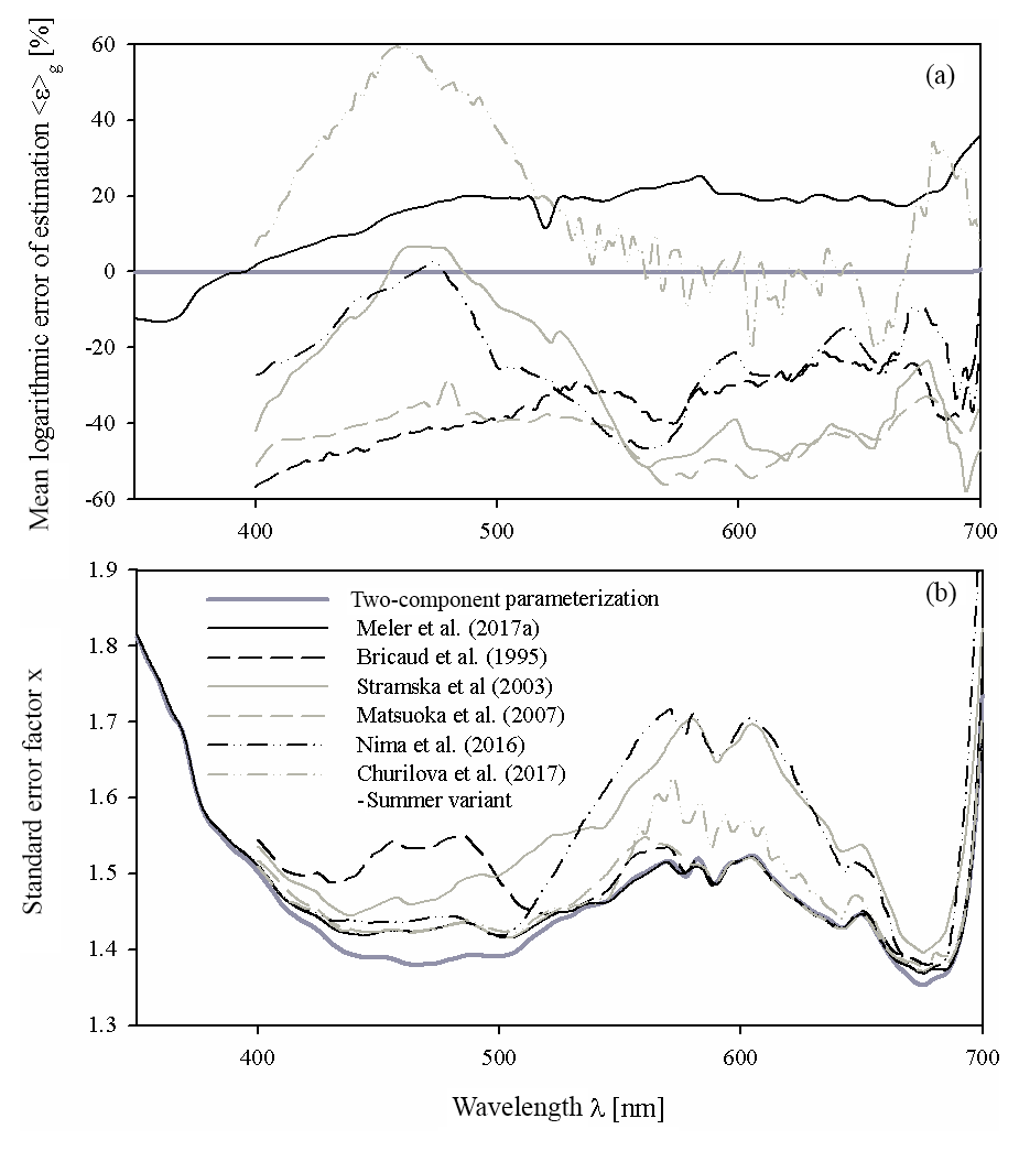
Figure 9 Comparison of the main characteristics of the estimation error logarithmic statistics calculated for various parameterizations of phytoplankton absorption coefficients: (a) the mean logarithmic errors of estimation 〈ε〉_g and (b) the standard error factor x. Different curves in these panels represent the two-component parameterization from this study, the preliminary parameterization according to Meler et al. (2017a) and selected examples of parameterizations gleaned from the literature (according to Bricaud et al., 1995; Churilova et al., 2017; Nima et al., 2016; Matsuoka et al., 2007; Stramska, 2003) (the legend is given in panel b). All these parameterizations were applied to our entire dataset.

Distinct differences between different months can also be visualized by plotting the mass-specific absorption coefficients $a_{\mathrm{ph}}^{\ast }$ at selected bands against chlorophyll a concentrations. Figure 6a and c illustrate such plots for 440 and 675 nm bands. Evident differences in the slopes of approximate curves for the selected four months can be seen. Although for May and March we obtain slopes of the $a_{\mathrm{ph}}^{\ast }$ vs. Tchl a relationships relatively close to those obtained for the whole dataset, quite different values are obtained for April and September.

3.2.2 Two-component parameterization

As already indicated in Sect. 3.1, there is a noticeable variation in the proportion between Tchl a and the concentrations of other phytoplankton pigments in particular months of the year within our dataset (Fig. 3). This variability initially indicated the limitations that may crop up when the chlorophyll a concentration is used as the only variable for parameterizing the spectra of a_ph(λ). Such limitations became clear when we recorded the differences between the parameterizations matched to the data from selected months. As a step towards improving the accuracy of a_ph parameterization, while retaining the relative simplicity of the mathematical formalism used, we decided to search for one additional variable. Different candidates for this variable were tested: various ratios between concentrations of different groups of accessory pigment concentrations (Tchl b, Tchl c, PSC, PPC, their partial sums and the sum ΣC_i) and Tchl a. As a result of these tests we found that the best for this particular purpose was the ratio of all accessory pigments to chlorophyll a (ΣC_i∕Tchl a). The new expression that approximates a_ph(λ) by treating it as a function of two variables at each light wavelength can be written as follows (more details on how the new formula was derived are given in Appendix B):

$$\begin{array}{}\text{(4)}& a_{\mathrm{ph}}\left(\mathit{\lambda }\right)=A_{\mathrm{0}}\left(\mathit{\lambda }\right)\cdot e^{K\left(\mathit{\lambda }\right)\cdot \frac{\sum C_i}{\mathrm{Tchl}a}}\cdot \mathrm{Tchl}{a}^{E\left(\mathit{\lambda }\right)}.\end{array}$$

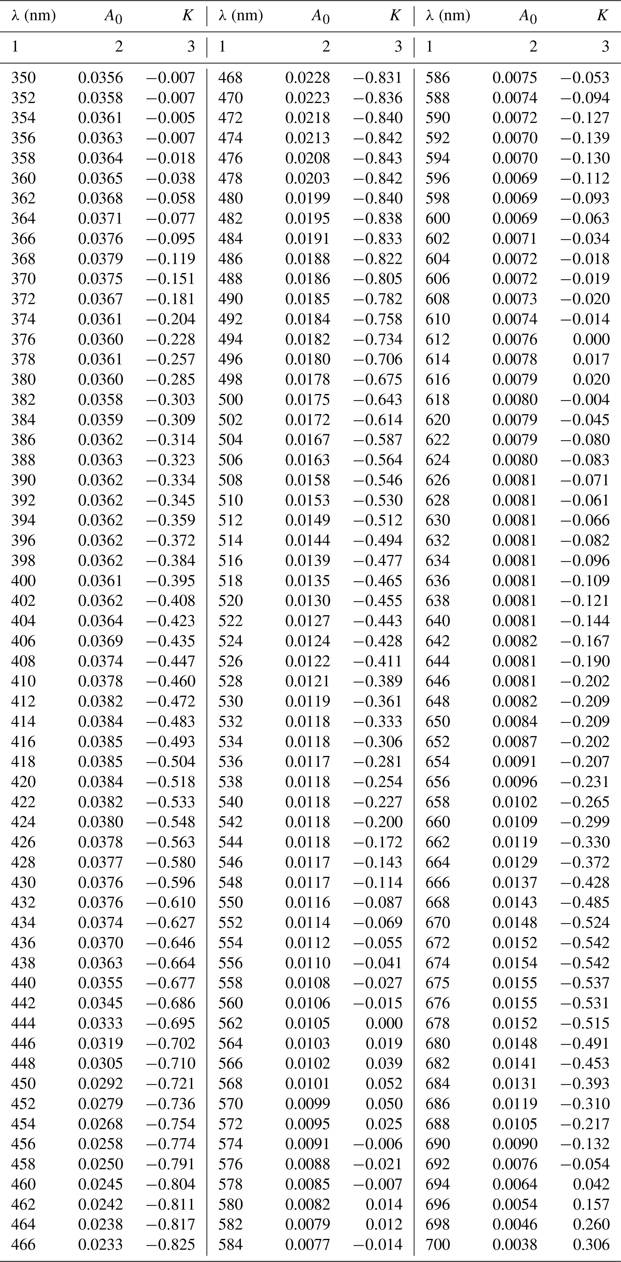
The numerical coefficients of the new parameterization, i.e. A₀(λ)(m² mg⁻¹) and K(λ) (no units), are summarized in Table A3 in Appendix A (with a spectral resolution of 2 nm). Note that coefficient E(λ) (no units) takes the same values as those in the general variant of the one-component parameterization. Note, too, that the product of the new coefficient A₀(λ) and the exponential function appearing in Eq. (4) allows one, with the adopted value of the ratio ΣC_i∕Tchl a, to calculate the value corresponding to coefficient A(λ) from the parameterization given by Eq. (3a). We define this product as

$$\begin{array}{}\text{(5)}& A{}^{\prime }\left(\mathit{\lambda },{\displaystyle \frac{\sum C_i}{\mathrm{Tchl}a}}\right)=A_{\mathrm{0}}\left(\mathit{\lambda }\right)\cdot e^{K\left(\mathit{\lambda }\right)\cdot \frac{\sum C_i}{\mathrm{Tchl}a}}.\end{array}$$

Spectral values of the new coefficients of Eq. (4) (coefficients A₀(λ) and K(λ)) are shown in Fig. 7a, and Fig. 7b illustrates the family of A^′(λ, ΣC_i∕Tchl a) curves plotted for some values of ΣC_i∕Tchl a in our database.

As in the case of single-variable parameterizations, example families of $a_{\mathrm{ph}}^{\ast }$ curves are now presented for the new two-component parameterization (Fig. 8) for two values of ΣC_i∕Tchl a, i.e. 0.47 and 0.88, corresponding to the 10th and 90th percentiles from the observed distribution of that ratio. There are conspicuous differences in this respect between both the values and the shapes of the $a_{\mathrm{ph}}^{\ast }$ spectra. As expected, the new two-component parameterization generally predicts lower values of $a_{\mathrm{ph}}^{\ast }\left(\mathit{\lambda }\right)$ for lower values of ΣC_i∕Tchl a than for higher ones. If we assume a low proportion of accessory pigments, i.e. for $\mathrm{\Sigma }{C}_i/\mathrm{Tchl}a=\mathrm{0.47}$ and Tchl a increasing from 0.3 to 100 mg m⁻³, the colour index falls from 2.69 to 1.72, i.e. by a factor of 1.57. In contrast, if we assume a higher proportion of accessory pigments (=0.88), the colour index decreases by the same factor (1.57) but from a higher starting value of 2.85, to 1.82. However, none of these differences are as distinct as those between the families of $a_{\mathrm{ph}}^{\ast }$ curves, drawn earlier according to the one-component parameterizations obtained for particular months (Fig. 5). Generally speaking, we can expect the use of the two-component parameterization to introduce an additional “degree of freedom” to the description of the variability of parameterized light absorption spectra. But it also seems likely that even with the new two-component parameterization, it will not be possible to explain all the differences manifested by the monthly one-component parameterizations. This intuitive expectation can be quantitatively checked by analysing in detail the estimation errors calculated for different variants of the parameterizations.

3.3 Estimation errors of the different variants of parameterizations

We performed an extensive analysis of the errors arising out of the different variants of the proposed approximation formulas (analysis of estimation errors). Different cases were considered: the formulas were tested on the whole dataset as well as on data from particular months only. In our analyses we used both the arithmetic statistics of relative errors and also so-called logarithmic statistics, as these are generally appropriate when the variation in tested/estimated quantities spans several orders of magnitude. Below we present the most important results of these analyses.

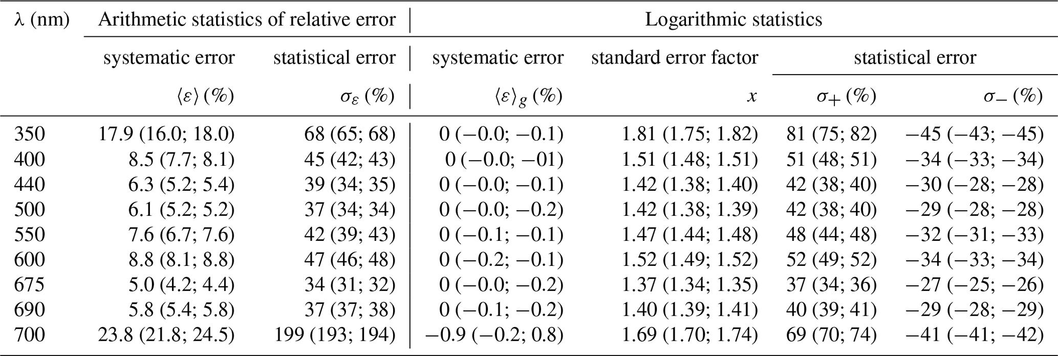
Table 3 Statistics of estimation errors^* of coefficient a_ph(λ) in selected spectral bands when the different variants of the parameterization derived in this study were applied to the entire dataset (n=1002). The calculated values are given for three scenarios: when the general variant of the one-component parameterization was used; when variants specific to individual months were chosen (the first alternative value is given in parentheses); and when the two-component parameterization was used (the second alternative value is given in parentheses).

^* Arithmetic statistics of the relative error:
mean of the relative error (representing the systematic error according to arithmetic statistics): $\langle \mathit{\epsilon }\rangle =N^{-\mathrm{1}}\sum _{i=\mathrm{1}}^N{\mathit{\epsilon }}_i$ , where $\mathit{\epsilon }=\frac{(P_i-O_i)}{O_i}$, O_i represents observed/measured values and P_i represents predicted/estimated values;
standard deviation of the relative error (representing the statistical error according to arithmetic statistics): ${\mathit{\sigma }}_{\mathit{\epsilon }}=\sqrt{\frac{\mathrm{1}}{N}\left(\sum _{i=\mathrm{1}}^N{\left({\mathit{\epsilon }}_i-\langle \mathit{\epsilon }\rangle \right)}^{\mathrm{2}}\right)}$.

Logarithmic statistics:
the mean logarithmic error (representing the systematic error according to logarithmic statistics): $\langle \mathit{\epsilon }{\rangle }_g={\mathrm{10}}^{〈\log \left(\frac{P_i}{O_i}\right)〉}-\mathrm{1}$, where $〈\log \left(\frac{P_i}{O_i}\right)〉$ is the mean of $\log \left(\frac{P_i}{O_i}\right)$;
the standard error factor (the quantity which allows the range of statistical errors to be calculated according to logarithmic statistics): $x={\mathrm{10}}^{{\mathit{\sigma }}_{\log }}$, where σ_log is the standard deviation of the set $\log \left(\frac{P_i}{O_i}\right)$;
statistical logarithmic errors (representing the range of statistical errors according to logarithmic statistics): ${\mathit{\sigma }}_{-}=\frac{\mathrm{1}}{x}-\mathrm{1}$, ${\mathit{\sigma }}_{+}=x-\mathrm{1}$.

Table 4 Selected characteristics of the estimation error logarithmic statistics calculated according to different parameterizations and for particular months: March, April, May and September (the numbers of data considered were 174, 96, 201 and 211, respectively).

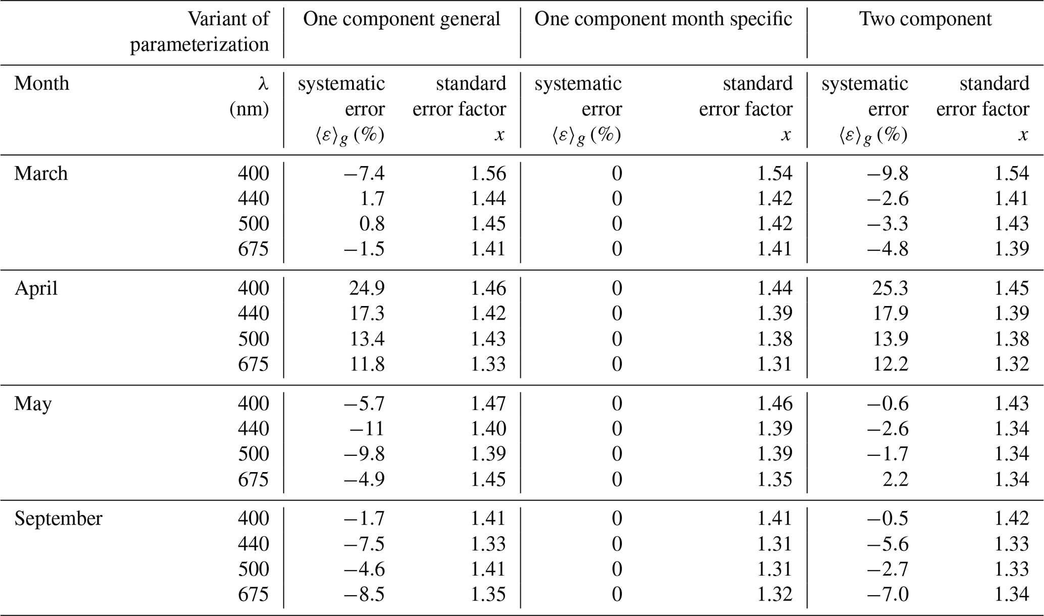
Table 3 sets out the statistics of estimation errors when different variants of the parameterizations were tested on the whole dataset. Three scenarios were considered: first, when the general variant of the parameterization was used to calculate absorption coefficients; second, when the relevant variants of monthly parameterizations were used, depending on the month of data acquisition; and third, when the two-component parameterization was used (the values for the second and third scenarios are given in parentheses). All these results are given for nine light wavelengths chosen to cover the spectral range under consideration and include the characteristic maxima of light absorption by chlorophyll a. We found that the estimation errors of coefficients a_ph obtained using the general parameterization were relatively stable from 400 to 690 nm. In this range, the systematic error according to arithmetic statistics remains at the relatively low level of 5 %–9 %, while the statistical error varies from 34 % to just over 50 %. Because the general parameterization was developed using linear least-squares regression applied to the logarithms of Tchl a and a_ph, the systematic error according to logarithmic statistics is always equal or very close to zero. The standard error factor x, which enables the statistical error range according to logarithmic statistics to be determined (by multiplying or dividing by its value – formulas are given as a footnote to Table 3), varies between 1.37 and 1.52 for wavelengths from 400 to 690 nm; values are higher only at the edges of the spectral range under investigation. This means that the statistical error according to logarithmic statistics in the 400–690 nm range varies from −34 % to 52 %; if the entire spectral range is considered, it varies from −45 % to 81 %. For the second scenario of calculations done over the entire dataset, i.e. when different monthly parameterization were used on an entire dataset, the errors are only slightly lower than the previous ones. Applying logarithmic statistics to this scenario leads to a standard error factor varying from 1.34 to 1.49 in the 400–690 nm range and taking values of ≤1.75 at the edges of this range. Hence, the statistical error according to logarithmic statistics in the 400–690 nm range varies from −33 % to 49 % and from −45 % to 75 % if the entire spectral range is considered. In the third scenario, i.e. when the new two-component parameterization was applied to a whole dataset, we found estimation errors to lie generally between the errors of the first and second scenarios. In terms of logarithmic statistics, again, as expected, the systematic errors are close to zero, and the standard error factor in the 400–690 nm range varies from 1.35 to 1.52. A detailed comparison of the results obtained indicates that applying the two-component parameterization to a whole dataset leads to a small but noticeable reduction in the errors compared with use of the general version of the one-component parameterization (Eq. 3a) only in the 390–530 and 665–685 nm spectral ranges. These are the ranges in which significant differences in the family of A^′(λ, ΣC_i∕Tchl a) curves have been observed (Fig. 7b). However, comparison of the estimation errors associated with the two-component parameterization with the scenario of using monthly variants of the one-component parameterization slightly favours the latter.

The above estimation errors were calculated over the entire available dataset. Therefore, these results do not address the question of how much more accurate the results might be if different variants of parameterization were tested on data from just one particular month. Table 4 gathers some results which address the latter question. It lists results obtained for data subsets limited to four separate months and to light wavelengths representing only selected bands where the phytoplankton absorption is relatively high. Additionally, for brevity, only certain characteristics of the logarithmic statistics are presented. We generally found that using the monthly parameterization instead of a general variant for individual months often reduces the level of statistical error according to both arithmetic and logarithmic statistics by only a small amount, although it may have a significant impact by strongly reducing the systematic error. Applying the general variant of the parameterization to particular months may overestimate or underestimate the values of coefficients a_ph by a few percent to as much as 30 % and more in extreme situations (up to 25 % for the spectral bands shown in Table 4). If we take the case of April, the general parameterization variant overestimates a_ph(λ) by ca. 12 % to 34 %, depending on the light wavelength. For September, on the other hand, a_ph(λ) is underestimated by ca. 2 % to 9 % in the majority of the visible range. In other months a_ph(λ) may be overestimated in some spectral ranges and underestimated in others. In contrast, according to expectations, using appropriately matched monthly parameterizations in all of these cases enables one to eliminate the systematic error according to logarithmic statistics and to significantly reduce the systematic error of the arithmetic statistics. Applying the two-component parameterization rather than the general variant of the one-component parameterization usually leads to a reduction in the statistical errors in the vicinity of phytoplankton absorption peaks. The systematic error is reduced only in two of the months analysed (May and September), while in the others, there is no influence or even a slight increase (April and March).

3.4 Comparison with selected examples of parameterizations from the literature

So far, when discussing our own results, we have referred only to the classic version of the parameterization given by Bricaud et al. (1995). Now we shall briefly compare our results with other examples of parameterizations from the literature. In Fig. 5d and e we have plotted the coefficients of the parameterization by Bricaud et al. (1995), as well as coefficients of four other variants obtained for different marine environments by different authors: Stramska et al. (2003), Matsuoka et al. (2007), Nima et al. (2016) and Churilova et al. (2017). These examples were chosen from among the many known in the literature, in order to illustrate the possible variability occurring between coefficients of different parameterizations that were originally matched to different datasets. In the case of coefficients A, all the spectral shapes presented in Fig. 5d generally reflect the characteristic absorption maxima in the blue and red spectral ranges. Quantitatively, however, there are significant differences between these examples, the largest being in the wavelength range from about 400 to 480 nm. Interestingly, such a range of coefficient A variability resembles the one we obtained with our own Baltic data when we developed separate variants of the one-component parameterization for individual months (Fig. 5a). With regard to the values of coefficients E, the literature examples presented in Fig. 5e differ significantly from each other and all exhibit a distinct variation in values across the spectrum. According to these literature sources, coefficients E can take values from less than 0.5 to even more than 1 in different spectral ranges. In our analyses we also found spectral variations in E values but only for parameterization variants that were matched to the data from separate months; on pooling all our data, we found that the resulting spectral shape of coefficient E was relatively flat (with values between 0.8 and 0.9 for the general parameterization variant) (Fig. 5b). The fact that the various literature parameterizations clearly differ in their coefficients E can be additionally illustrated by different slopes of curves plotted on graphs showing estimated dependences of specific absorption coefficients a_ph*(440) and a_ph*(675) as functions of Tchl a (Fig. 6b and d). In addition to the examples mentioned earlier, we also plotted curves according to Staehr and Markager (2004) as examples representing a wide range of Tchl a. Again, we would like to point out that the pattern of different slopes among literature examples resembles the differences we obtained from analysing the data for different months.

As a final aspect of this brief comparison, Fig. 9 shows the main characteristics of the logarithmic statistics describing the accuracy of the formulas chosen from the literature when they were applied to calculate coefficient a_ph of our whole dataset. This was only done for illustrative purposes – in no way was it an attempt to validate our results. As may be seen from Fig. 9a, all the literature formulas compared reveal significant systematic errors when they were tested on our dataset. The systematic estimation errors of a_ph(λ) in the classic parameterization according to Bricaud et al. (1995) range from −57 % to −21 % over almost the entire spectral range. Other examples show significant systematic errors at least in some portions of the light spectrum analysed (from almost −60 % to about +60 % at some cases). In Fig. 9a we also plotted systematic errors calculated now for our own, previous preliminary version of the Baltic Sea parameterization (Meler et al., 2017a). We now see that, apart from the UV range, values of a_ph are generally overestimated by up to 20 % and more by this earlier version of the formula. With regard to the standard error factor, we can see that only some of the literature examples in the vicinity of phytoplankton light absorption peaks achieve similarly low values as represented by our new two-component parameterization. But since for the total estimation accuracy the contributions of both systematic and statistical errors have to be taken into account, one can expect that overall, none of the literature examples can attain the accuracy that we achieved by matching our new parameterizations to our own dataset.

4 Final remarks

The empirical material for this work was acquired in a relatively small geographical area, mainly the southern Baltic Sea. However, because it was gathered in various parts of this basin, from coastal areas to open waters, and at different times of the year, the recorded light absorption coefficients and concentrations of phytoplankton pigments have large ranges of variability, in both cases reaching almost 3 orders of magnitude. Based on such a dataset, it was possible to derive a number of new variants of the parameterization of coefficient a_ph: they should be treated as simplified and practical relationships of a local character, tailored to the specifics of the target environment. The new empirical formulas include classic one-component parameterizations, where the only variable is the concentration of chlorophyll a. Parameterizations of this type have been developed both as a general version, i.e. one matched to all the data collected in different periods of the year, and in the form of separate variants adjusted to the individual months of data collection. Importantly, we found that the coefficients of monthly variants could differ from each other very significantly, thus indirectly reflecting the annual variation in the proportions between chlorophyll a and other photosynthetic or photoprotective pigments. The paper also presents a new, slightly more complex form of parameterization that uses one additional variable: the ratio of the concentrations of accessory pigments to the concentration of chlorophyll a.

With all the variants of this parameterization, spectra of coefficient a_ph can be estimated fairly simply and with few requirements as to input data. Such estimates can be made over a wide spectral range (from 350 to 700 nm) and with a high spectral resolution (1 nm). It should be borne in mind, however, that the accuracy of such estimates is obviously limited. For example, the application of the general version of the one-component parameterization to all our data covering different periods of the year understandably leads to practically zero systematic error of this estimate, although a significant statistical error remains. The latter may be characterized by standard error factors from 1.37 to 1.51 in the vast majority of the spectral ranges tested. However, since the real values of a_ph vary in Baltic Sea conditions over almost 3 orders of magnitude, even an estimation accuracy such as this appears satisfactory. Our study has also shown that further improvement in the accuracy of the approximate description of a_ph spectra is possible, at least in some applications. In the case of datasets acquired at different times of the year, such an improvement can be achieved by using either “dynamically selected” monthly variants of parameterizations, or, when pigment composition data are available, by using the new two-component parameterization. In the case of data limited to particular months, it is possible to prevent the occurrence of significant systematic errors especially by using the appropriately selected monthly parameterization.

An important qualitative observation from our analyses is that the new variants of monthly parameterizations have a range of variability of coefficients similar to that between the different literature parameterizations established on the basis of data from diverse aquatic environments. This particular observation reminds us that all such parameterizations are always quite far-reaching simplifications of relationships occurring in nature. The variability of these relationships that we recorded throughout the year in the Baltic Sea seems to indicate that only the use of a much more elaborate mathematical apparatus, using a much larger number of variables describing the composition of pigments and other features of the phytoplankton population, could further and more radically improve the accuracy of the spectral description of the light absorption coefficient (see, e.g., the multi-component models presented earlier in the papers by Woźniak et al., 1999, 2000a, b; Majchrowski et al., 2000; Ficek et al., 2004). In our opinion, however, the practical value of the simple parameterizations presented in this work should be seen in the opportunities for applying them to the development of various methods and algorithms, whose specificity from the very beginning requires the use of simplifications.

Appendix A

The spectral coefficients of certain variants of the parameterizations obtained in this work are given in the tables below with either 2 or 5 nm spectral steps. The values of the coefficients with 1 nm resolution and for other cases not presented below are available from the authors on request.

Table A1 Spectral coefficients A and E of the one-component parameterization described by Eq. (3a) in its general variant (i.e. the variant obtained when all data, regardless of the month of acquisition, were taken into account) and the corresponding determination coefficients R².

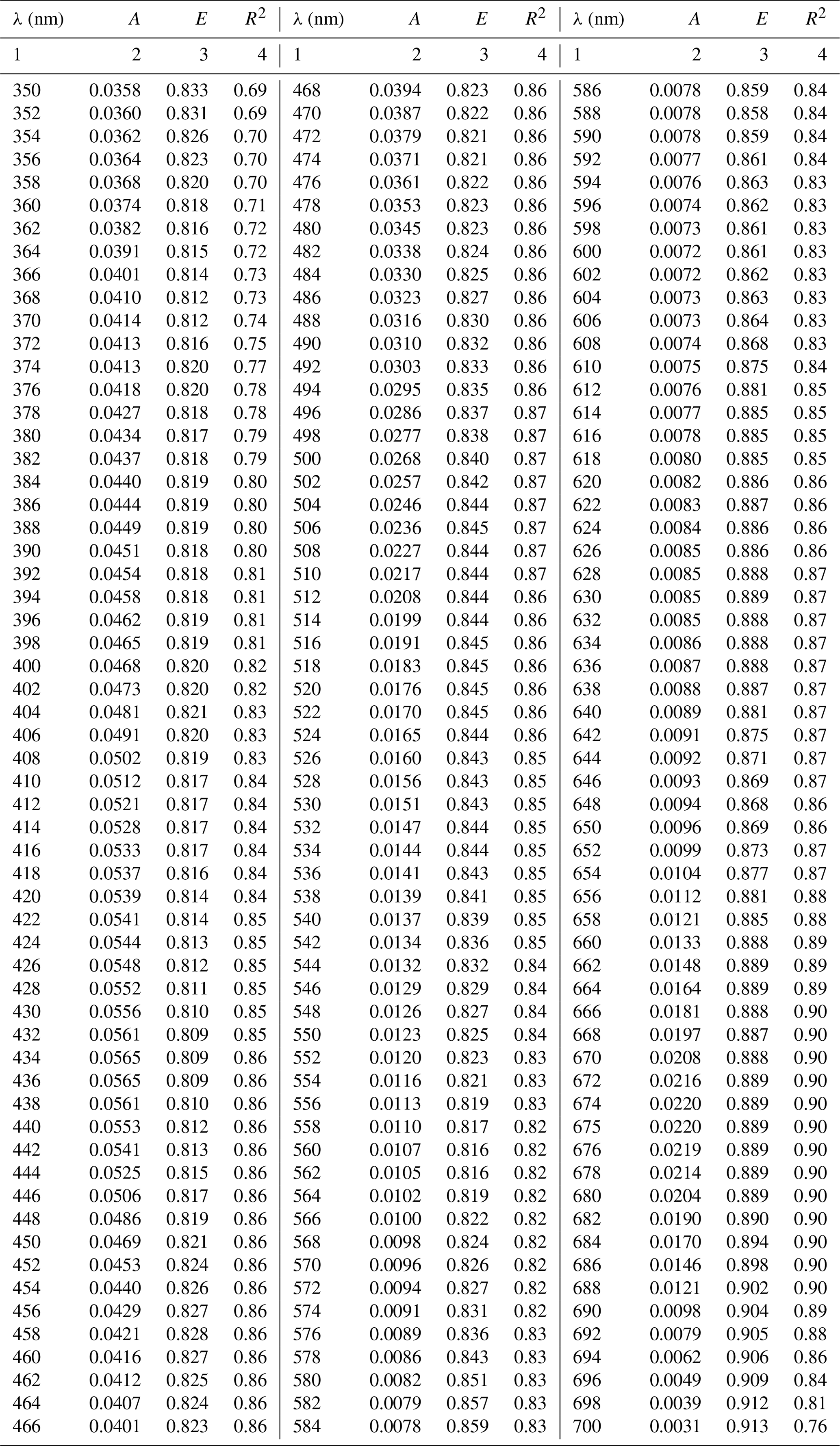
Table A2 Spectral coefficients A and E of the one-component parameterization described by Eq. (3a) in its variants obtained in selected months and the corresponding determination coefficients R².

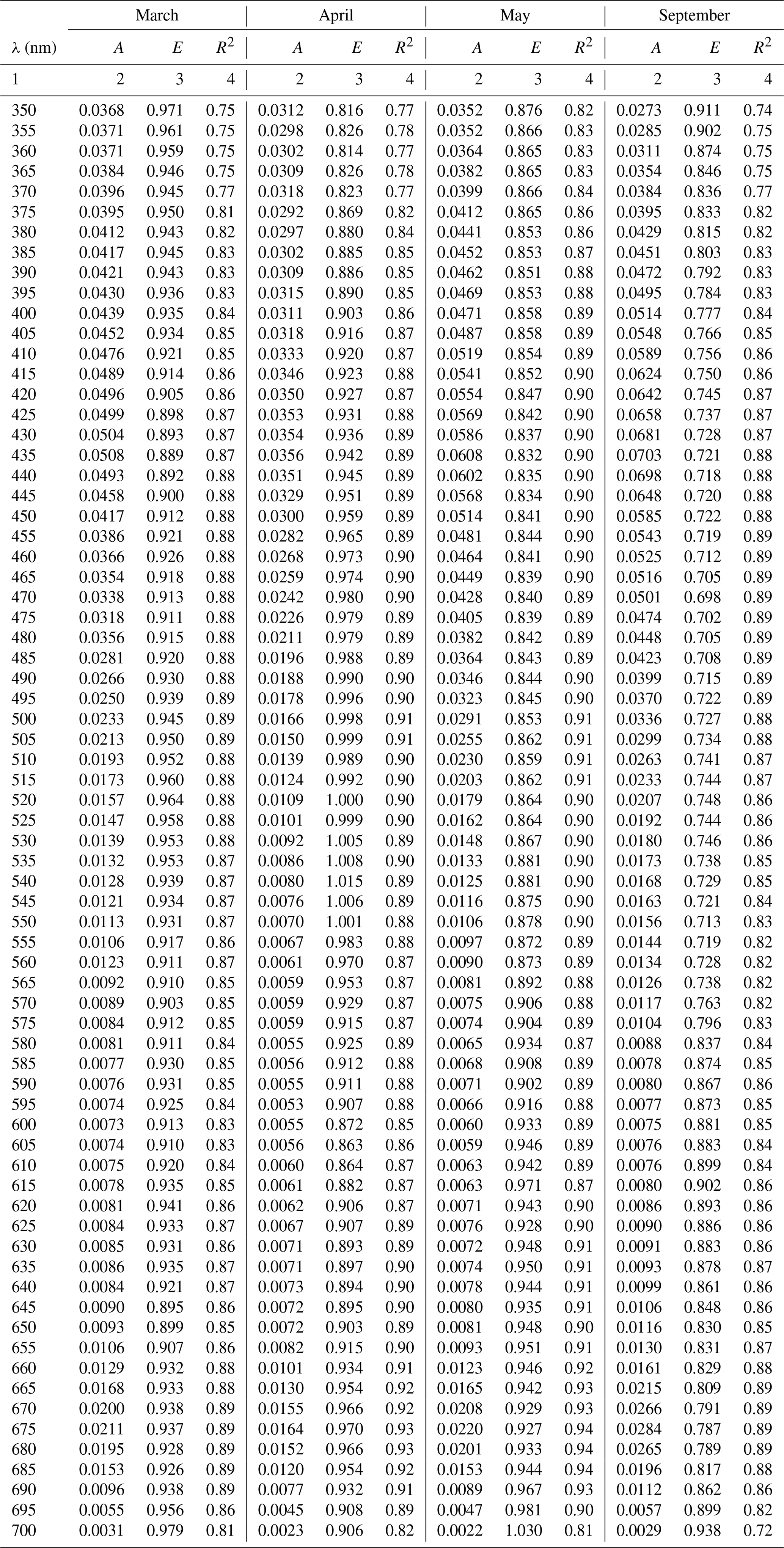
Table A3 Spectral coefficients A₀ and K of the two-component parameterization described by Eq. (4). The other coefficient E is the same as in the case of the one-component parameterization (see Table A1).

Appendix B

In order to derive the two-component parameterization, the relationship described earlier by Eq. (3a) was treated as a first, intermediate stage in its construction (the examples are plotted at two wavelengths in Fig. B1a and b). To distinguish between them, the values calculated according to Eq. (3a) are now denoted a_ph(λ)_cal, whereas the actually measured values of the absorption coefficient are a_ph(λ)_m. In the next step, the relationship between the ratio a_ph(λ)_cal∕a_ph(λ)_m and the ratio of the sum of accessory pigments to the concentration of chlorophyll aΣC_i∕Tchl a was analysed. Figure B1c and d illustrate the frequency distributions of the ratio a_ph(λ)_cal∕a_ph(λ)_m, while Fig. B1e and f show the relationships between the ratios a_ph(λ)_m∕a_ph(λ)_cal and ΣC_i∕Tchl a. Despite the large dispersion of individual data points on the latter two panels, the general tendency for the logarithm of a_ph(λ)_m∕a_ph(λ)_cal to decrease with increasing ΣC_i∕Tchl a is evident. This tendency can be approximated by a linear function, which effectively allows one to establish coefficients of an approximate exponential relationship between the two ratios investigated:

$$\begin{array}{}\text{(B1)}& {\displaystyle \frac{a_{\mathrm{ph}}(\mathit{\lambda }{)}_{\mathrm{cal}}}{a_{\mathrm{ph}}(\mathit{\lambda }{)}_{\mathrm{m}}}}=f\left({\displaystyle \frac{\sum C_i}{\mathrm{Tchl}a}}\right)={\mathrm{const}}_{\mathrm{1}}\left(\mathit{\lambda }\right)e^{{\mathrm{const}}_{\mathrm{2}}\left(\mathit{\lambda }\right)\frac{\sum C_i}{\mathrm{Tchl}a}}.\end{array}$$

Relationships of this form were determined over the entire spectral range (350–700 nm) with a step of 1 nm. Obviously, the determination coefficients R² of the approximations are low, but this procedure generally permits additional information on the influence of pigment composition on the ultimate values of a_ph to be taken into account. Having the statistical dependences described by first stage Eq. (3a) and second stage Eq. (B1) to hand, a new expression can be written that approximates a_ph(λ) by treating it as a function of two variables at each light wavelength – chlorophyll a concentration (Tchl a (mg m⁻³)) and the ratio of the sum of the concentrations of the other accessory pigments to chlorophyll a (ΣC_i∕Tchl a):

$$\begin{array}{}\text{(B2)}& a_{\mathrm{ph}}\left(\mathit{\lambda }\right)=A_{\mathrm{0}}\left(\mathit{\lambda }\right)\cdot e^{K\left(\mathit{\lambda }\right)\cdot \frac{\sum C_i}{\mathrm{Tchl}a}}\cdot \mathrm{Tchl}{a}^{E\left(\mathit{\lambda }\right)}.\end{array}$$

The numerical coefficients of the newly obtained parameterization, i.e. A₀(λ) (m² mg⁻¹) (where $A_{\mathrm{0}}\left(\mathit{\lambda }\right)=A\left(\mathit{\lambda }\right)/{\mathrm{const}}_{\mathrm{1}}\left(\mathit{\lambda }\right))$ and K(λ) (no units) (where $K\left(\mathit{\lambda }\right)=-{\mathrm{const}}_{\mathrm{2}}\left(\mathit{\lambda }\right))$, are summarized in Table A3 in Appendix A. Coefficient E(λ) (no units) takes the same values as those in the general variant of the one-component parameterization.

Figure B1 (a, b) Relations between measured coefficients of absorption by phytoplankton (denoted by a_ph(λ)_m) and chlorophyll a concentrations for two light wavelengths (400 and 675 nm) and their functional approximations according to Eq. (3a) (the equations are given in the panels); (c, d) frequency distribution histograms of the ratio of calculated and measured absorption coefficients (a_ph(λ)_cal∕a_ph(λ)_m); (e, f) relations between the ratio a_ph(λ)_cal∕a_ph(λ)_m and the pigment concentration ratio ΣC_i∕Tchl a and their functional approximations (the equations are given in the panels).