A surface kinematics buoy (SKIB) for wave–current interaction studies

Global navigation satellite systems (GNSSs) and modern motion-sensor packages allow the measurement of ocean surface waves with low-cost drifters. Drifting along or across current gradients provides unique measurements of wave–current interactions. In this study, we investigate the response of several combinations of GNSS receiver, motion-sensor package and hull design in order to define a prototype “surface kinematics buoy” (SKIB) that is particularly optimized for measuring wave–current interactions, including relatively short wave components that are important for air–sea interactions and remote-sensing applications. The comparison with existing Datawell Directional Waverider and Surface Wave Instrument Float with Tracking (SWIFT) buoys, as well as stereo-video imagery, demonstrates the performance of SKIB. The use of low-cost accelerometers and a spherical ribbed and skirted hull design provides acceptable heave spectra E(f) from 0.09 to 1 Hz with an acceleration noise level (2πf)⁴E(f) close to 0.023 m² s⁻³. Velocity estimates from GNSS receivers yield a mean direction and directional spread. Using a low-power acquisition board allows autonomous deployments over several months with data transmitted by satellite. The capability to measure current-induced wave variations is illustrated with data acquired in a macro-tidal coastal environment.

1 Introduction

Many devices have been developed to measure ocean waves, from in situ moored or drifting sensors to remote-sensing systems using optical or radar devices (COST Action 714 Working Group 3, 2005). Each measurement system has a specific range of applications defined by the required space and time resolution and coverage, water depth, and current speed. They have been very useful in studying upper-ocean processes or monitoring sea states for various applications. Among all these, surface buoys such as the Datawell Directional Waverider have been reference instruments for the estimation of the sea surface elevation frequency spectra from measurements of buoy acceleration. The combined horizontal and vertical accelerations give the first five angular moments of the directional spectrum that can be used to estimate the directional wave spectrum (Benoit et al., 1997). In conditions with strong currents, e.g., more than 1 m s⁻¹, it is usually impossible to measure waves with a moored surface buoy, due to the tension on the mooring line. This problem is avoided with drifting buoys, but the nature of the measurement is different. Drifting buoys will not measure long time series at the same location, but they can provide a unique along-section measurement of waves following the current (Pearman et al., 2014). Several devices such drifting buoys have been developed recently for different applications (Herbers et al., 2012; Reverdin et al., 2013; Thomson, 2012). With our focus on relatively short gravity waves, with a wavelength between 1 and 30 m, there is a trade-off between the size of the device and its response to the waves. In practice, the buoy cannot be too small so that it is easily found and recovered nor too large so that it follows the motion of these short gravity waves. Besides waves, the time evolution of the buoy position can also be used to estimate surface currents in cases where the wind force on the buoy is negligible.

Herbers et al. (2012) proposed a compact and low-cost 45 cm diameter GPS-tracked drifting buoy. This buoy uses a GPS receiver for absolute position tracking. Herbers et al. (2012) compared it with Datawell and found that the horizontal wave orbital displacements are accurately resolved, although the vertical sea surface displacements were not well resolved by standard GPS measurements, requiring an external high-precision antenna to be attached to the drifter.

Thomson (2012) developed the Surface Wave Instrument Float with Tracking (SWIFT), a multi-sensor drifter buoy. This instrumented spar buoy has a 0.3 m diameter and 2.15 m height and has been designed to measure wind, waves, whitecap properties, and underwater turbulence and current profiles. Wave measurements are derived from the phase-resolving GPS, which contains the wave orbital motions relative to the earth reference frame. The relatively large size of the buoy is needed for the other measurements; however, the size and shape result in a very weak response for wave frequencies above 0.4 Hz. Obviously, the SWIFT buoy design has other benefits, such as the use of an acoustic Doppler current profiler that allows us to investigate the effect of the vertical current shear on the waves (Zippel and Thomson, 2017).

Reverdin et al. (2013) developed a surface wave rider (called “Surpact”) to measure sea state and atmospheric sea level pressure as well as temperature and salinity at a small fixed depth from the surface. Surpacts use a floating annular ring (28 cm diameter) with a rotating axis across it, to which the instrumented tag is attached and uses the vertical acceleration to obtain the power spectrum between 0.2 and 2.2 Hz.

Our goal is to measure the response of surface gravity waves to horizontal current gradients, in order to better interpret airborne and satellite imagery of waves and current features (Kudryavtsev, 2005; Rascle et al., 2014, 2017). Further out, away from the coasts, it is now understood that surface currents are the main cause of the variability of wave properties on small spatial scales (Ardhuin et al., 2017; Quilfen et al., 2018) and more measurements are required to better understand the processes at play and improve on the parameterizations of numerical wave models (Ardhuin et al., 2009; van der Westhuysen et al., 2012).

In this context, most of the existing wave buoys are generally too large to properly respond to short gravity waves. We have thus developed a low-cost drifting buoy, the “surface kinematics buoy” (SKIB), specially developed for wave–current interaction studies. Its design, tests and validations are presented here. This paper is organized as follows. Section 2 presents the relations between parameters recorded by the various devices used in our study and the wave spectrum. Section 3 explains the design of SKIB and validation in the laboratory and in situ. Section 4 describes an example application to measurements of waves and currents, and conclusions follow in Sect. 5.

2 Measurable parameters and processing

For random wind waves, the variance of the sea surface elevation field can be described using the variance density spectrum E(f_r,θ) or the action density spectrum N(k,θ), where $N(k,\mathit{\theta })=E(f_{\mathrm{r}},\mathit{\theta })/\mathit{\sigma }$, $f_{\mathrm{r}}=\mathit{\sigma }/\left(\mathrm{2}\mathit{\pi }\right)$ is the intrinsic (relative) wave frequency and θ is the wave direction.

For linear waves, the wavenumber k is related to the intrinsic wave frequency, i.e., the frequency measured by a drifting buoy following the current:

$$\begin{array}{}\text{(1)}& {\displaystyle }{\mathit{\sigma }}^{\mathrm{2}}=gk\tanh \left(kD\right),\end{array}$$

where D is the water depth and g the acceleration of the gravitational force.

In the presence of a horizontal current vector U that is vertically uniform, the intrinsic frequency differs from the absolute frequency $f_{\mathrm{a}}=\mathit{\omega }/\left(\mathrm{2}\mathit{\pi }\right)$ observed in a reference frame attached to the solid Earth:

$$\begin{array}{}\text{(2)}& {\displaystyle }\mathit{\omega }=\mathit{\sigma }+\mathit{k}\cdot \mathit{U}.\end{array}$$

A near-surface shear would lead to an effective current that varies with the wavenumber (Stewart and Joy, 1974).

When drifting with the surface current vector (u,v), a surface buoy can measure the three components of the acceleration vector (a_x, a_y, a_z), the GPS horizontal Doppler velocities (u,v) and positions (x, y, z). In practice the accelerations and horizontal velocities have relatively low noise and can be used to measure waves. In our SKIB acquisition system, the GPS data are sampled at 1 Hz while the accelerometer is sampled at 25 Hz, and they are independent systems.

The spectra and co-spectra of these time series can provide the first five Fourier coefficients of the angular distribution, also known as angular moments: a₀(f_r), a₁(f_r), b₁(f_r), a₂(f_r) and b₂(f_r) (Kuik et al., 1988b; Longuet-Higgins et al., 1963). From that, it is possible to obtain the directional distribution of the spectrum E(f_r,θ) (Longuet-Higgins et al., 1963).

For completeness, here are how the spectra and co-spectra C_xy of two quantities x and y, with x or y replaced by h for heave and u or v for the horizontal velocity components, are linked to the angular moments:

$$\begin{array}{ll}{\displaystyle }& {\displaystyle }\left(\begin{array}{c}{a}_{\mathrm{1}}\left(f_{\mathrm{r}}\right)\\ b_{\mathrm{1}}\left(f_{\mathrm{r}}\right)\\ a_{\mathrm{2}}\left(f_{\mathrm{r}}\right)\\ b_{\mathrm{2}}\left(f_{\mathrm{r}}\right)\end{array}\right)=\underset{\mathrm{0}}{\overset{\mathrm{2}\mathit{\pi }}{\int }}\left(\begin{array}{c}\cos \mathit{\theta }\\ \sin \mathit{\theta }\\ \cos \mathrm{2}\mathit{\theta }\\ \sin \mathrm{2}\mathit{\theta }\end{array}\right)E(f_{\mathrm{r}},\mathit{\theta })d\mathit{\theta }/\underset{\mathrm{0}}{\overset{\mathrm{2}\mathit{\pi }}{\int }}E(f_{\mathrm{r}},\mathit{\theta })d\mathit{\theta }\\ \text{(3)}& {\displaystyle }& {\displaystyle }=\left(\begin{array}{c}{C}_{\mathrm{uh}}/\sqrt{C_{\mathrm{hh}}(C_{\mathrm{uu}}+C_{\mathrm{vv}})}\\ C_{\mathrm{vh}}/\sqrt{C_{\mathrm{hh}}(C_{\mathrm{uu}}+C_{\mathrm{vv}})}\\ (C_{\mathrm{uu}}-C_{\mathrm{vv}})/(C_{\mathrm{uu}}+C_{\mathrm{vv}})\\ \mathrm{2}{C}_{\mathrm{uv}}/(C_{\mathrm{uu}}+C_{\mathrm{vv}})\end{array}\right).\end{array}$$

From the first moments it is customary (Kuik et al., 1988a) to define a mean direction θ₁(f_r) and directional spread s_θ1(f_r):

$$\begin{array}{}\text{(4)}& {\displaystyle }& {\displaystyle }{\mathit{\theta }}_{\mathrm{1}}\left(f_{\mathrm{r}}\right)={\tan }^{-\mathrm{1}}\left(b_{\mathrm{1}}/a_{\mathrm{1}}\right),\text{(5)}& {\displaystyle }& {\displaystyle }{s}_{\mathit{\theta }\mathrm{1}}\left(f_{\mathrm{r}}\right)=\sqrt{\mathrm{2}\left(\mathrm{1}-\sqrt{a_{\mathrm{1}}^{\mathrm{2}}+b_{\mathrm{1}}^{\mathrm{2}}}\right)}.\end{array}$$

When only velocity measurements are available, one can only access E(f_r), a₂(f_r), b₂(f_r), which give the two following parameters:

$$\begin{array}{}\text{(6)}& {\displaystyle }& {\displaystyle }{\mathit{\theta }}_{\mathrm{2}}\left(f_{\mathrm{r}}\right)={\displaystyle \frac{\mathrm{1}}{\mathrm{2}}}{\tan }^{-\mathrm{1}}\left(b_{\mathrm{2}}/a_{\mathrm{2}}\right),\text{(7)}& {\displaystyle }& {\displaystyle }{s}_{\mathit{\theta }\mathrm{2}}\left(f_{\mathrm{r}}\right)=\sqrt{\mathrm{0.5}\left(\mathrm{1}-\sqrt{a_{\mathrm{2}}^{\mathrm{2}}+b_{\mathrm{2}}^{\mathrm{2}}}\right)}.\end{array}$$

We estimated the auto- and cross-spectra following Welch (1967), using Fourier transforms over time series of 5000 samples, with a 50 % overlap, and using a Hann window. The resulting spectra have a frequency resolution of 0.005 Hz and 24 degrees of freedom (12 independent windows and 11 overlapped windows).

Because the GPS and accelerometer have different sampling frequencies, the buoy displacements are linearly interpolated on the accelerometer sampling time steps. This is only required for the co-spectrum of the horizontal displacements C_uv(f) and quadrature spectra of horizontal and vertical displacements C_uh(f), C_vh(f).

Here we will focus on frequencies between 0.06 and 0.80 Hz for our investigation of current gradients. We will also discuss the full frequency range for a validation of the buoy behavior.

3 Buoy design and validation

3.1 Hull shape and constraints of deployment at sea

The hull shape is clearly important when resolving short wave components. The main drivers are the stability of the buoy. We typically want to have the top of the buoy stay above the water surface, in particular for GPS acquisitions and radio transmission. We also wish to avoid rotation of the buoy relative to the water around it, and finally the buoy has to be big enough to be visible for recovery and small enough to be easily handled and to follow the motion of short waves. One final driver is the overall cost of the buoy. Because they also measure whitecaps with a camera and turbulence in the water, the SWIFT buoys use a spar shape that is 1.8 m tall. Such a shape is not ideal for short wave measurements because it resonates for heave excitation at a frequency around 0.8 Hz.

With all these constraints in mind we found that a nearly spherical shape with ribs and an additional skirt provided a good water-following behavior, whereas spherical shapes performed more poorly. Three-dimensional printing was tested without much success due to the porosity of the printed material. For the small number of buoys that we needed we finally settled on glass spheres, for which we had other oceanographic uses for buoyancy in deep water moorings. The standard ribbed cage for these spheres (Figs. 1 and 2) was augmented by a 3 cm wide skirt, as shown in Fig. 2, providing a nice water-following capability.

Figure 1 Surface kinematic buoy (SKIB) (a) main electronics components: microcontroller board (EFM32 cortex M3), with data storage and wireless link; GPS board; Iridium board; STM accelerometer or SBG IMU Ellipse N. (b) SKIBs with top cover removed, showing the 25.4 cm diameter glass spheres used to seal all the electronic components.

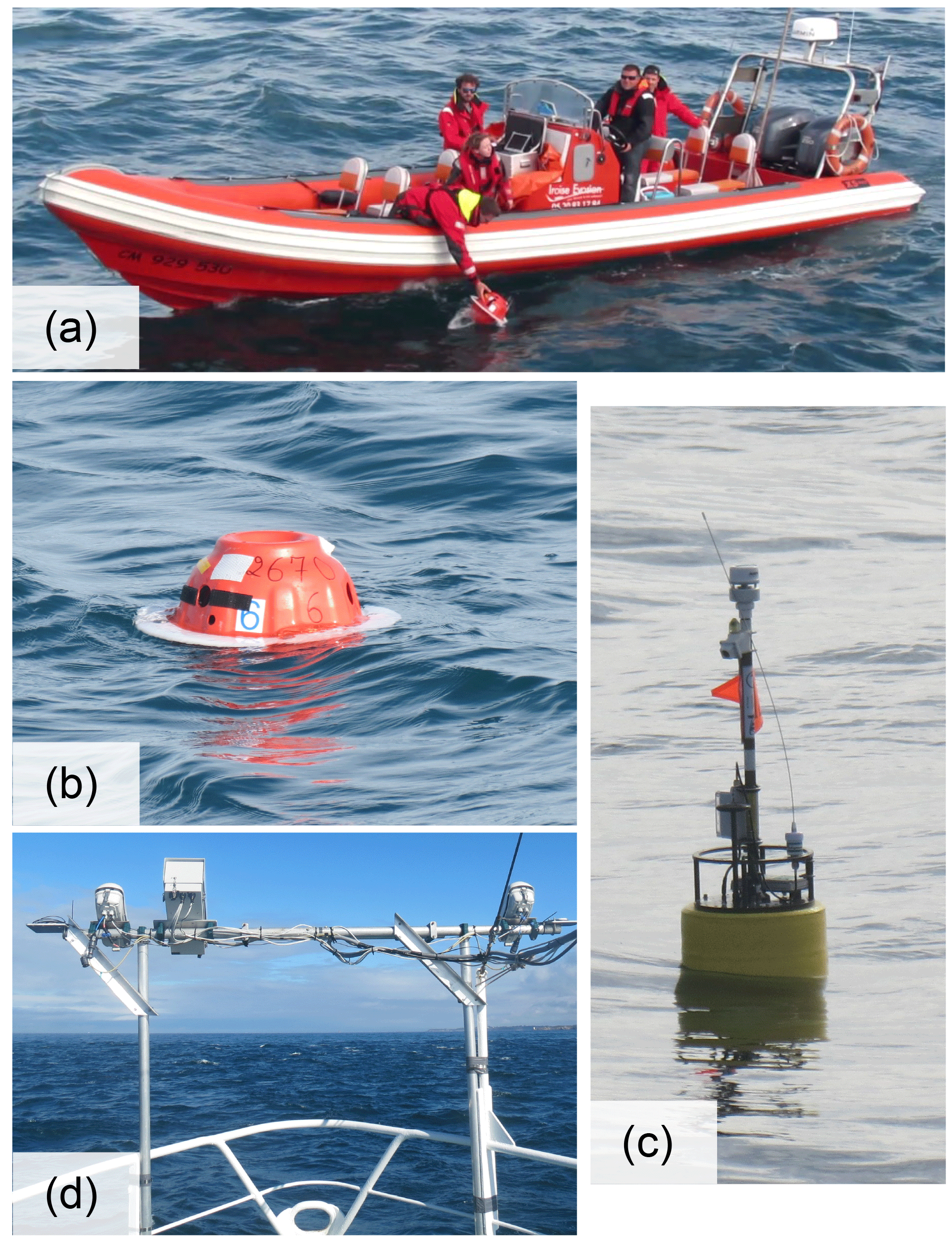
Figure 2 Sensors used during oceanographic campaigns for in situ validation. (a) SKIB deployment; (b) SKIB buoy; (c) SWIFT buoy; (d) stereo-video system.

3.2 SKIB electronics

The accelerometer and the GPS system are directly integrated in a general-purpose oceanographic Advanced Low Energy Electronic System (ALEES) board developed by Ifremer “Unité Recherche et Développements Technologiques” (RDT) especially for autonomous applications that need very low power consumption. This generic board uses a 32 bit microcontroller working at 48 MHz, a 1 Mb flash memory and 128 Kb RAM. The data are stored in a standard micro secure digital high-capacity (SDHC) memory card. The GPS and the accelerometer acquisitions are not synchronized and the acquisition rates are 1 and 25 Hz, respectively.

The integrated accelerometer is a STMicroelectronics model LIS3DH (when used with this configuration, this will be referenced as the SKIB STM buoy version), already incorporated in the ALEES board for other uses, namely the detection of strong motions for underwater sensors. This low-cost (less than USD 2) component was chosen for its very low power use: between 2 and 6 µA at 2.5 V.

A specific board was designed to control the GPS acquisition and send the buoy position via the Iridium board. We typically programmed the buoy to send position messages every 10 min, in order to be able to find the instruments at sea in highly variable currents. The ALEES and GPS boards can be controlled by a Zigbee wireless link. This wireless link also allows the user to set up the buoy and to recover the data without opening the glass spheres, allowing the system to power on and off.

All the system, including the electronic boards, battery pack and antennas (Zigbee, GPS, Iridium) are mounted inside a 25.4 cm diameter glass sphere, which is vacuum-sealed (see Fig. 1). Standard prices for all the parts in the year 2015 were about EUR 1100 for all electronics, half of which is for the Iridium and GPS equipment and another EUR 1100 of which is for the hull and mounts inside of the hull. That expensive choice of the hull was, in our case, justified by a possible reuse for other oceanographic applications.

For a detailed validation we have also integrated a more accurate sensor in two of the SKIB buoys (this is now referred to as the SKIB SBG buoy version). In those buoys an SBG Ellipse inertial measurement unit (IMU) was used, set to an acquisition rate of 50 Hz. However, this sensor significantly increases the equipment cost and power consumption, with a unit price typically above USD 4000.

3.3 Laboratory tests and in situ validation

Buoy testing started with the verification of the expected acceleration accuracy in a wave tank, followed by a comparison with in situ measurements with a reference wave buoy.

The laboratory tests were very useful for testing various hull shapes, from spheres to short cylinders. These led to the addition of the plastic skirt that effectively removes rotations around the horizontal axes, with a limited impact on the water-following capacity for short wave components. This final design has a heave transfer function of almost 1 up to 0.8 Hz, decreasing to 0.6 at 1 Hz, as established in wave basin tests (Thomas, 2015). This extends the useful range of buoys such as Datawell Waveriders or SWIFTs to a high frequency. For in situ validation, the SKIB buoy was deployed drifting within 200 m of a MkIII Datawell Directional Waverider of 70 cm diameter, moored in a region of weak currents with a mean water depth of 60 m at 48.2857^∘ N, 4.9684^∘ W. This Waverider buoy is part of the permanent CEREMA wave buoy network, with the World Meteorological Organization number 62069 (Ardhuin et al., 2012). This buoy provides measurements of the first five moments for frequencies of 0.025 to 0.580 Hz, based on accelerometer data.

Contrary to Herbers et al. (2012) who strapped their new acquisition system on a Waverider buoy, we wanted to validate the full system, including the hull response. As a result the different sensors do not measure the same waves (with the same phases) but should be measuring the same sea state, i.e., the same spectrum, moments and derived parameters.

The test presented here was performed on 21 September 2016, from 10:44 to 11:56 UTC, following a similar test in 2015 with only a SKIB and a with a different GPS receiver but the same hull and a Datawell Waverider. The results were very similar. In the 2016 experiment, we also deployed a SWIFT buoy (Thomson, 2012) and a ship-mounted stereo-video wave system (Benetazzo et al., 2016). Pictures of all these systems as used during the experiment are shown in Fig. 2.

The SWIFT model used is shown in the water in Fig. 2c. It uses a GPS receiver integrated with an IMU (Microstrain 3DM-GX3-35), a Doppler velocity profiler (Nortek AquadoppHR), an autonomous meteorological station ultrasonic anemometer (AirMar PB200), a digital video recorder system and a real-time tracked radio frequency transmitter. The wave spectra for each 10 min burst are calculated as the ensemble average of the fast Fourier transform of 16 sub-windows with 50 % overlap, which results in 32 degrees of freedom and a frequency bandwidth df=0.0117 Hz in the range $\mathrm{0.05}<f<\mathrm{0.5}$. The IMU data give information about the tilt and horizontal rotation, as well as accelerations, of the SWIFT as it follows wave motions. Note that the hull shape of the SWIFT follows displacements and velocities at the sea surface but not surface slopes. Hence, only velocities and accelerations are used in wave processing. Post-processing of the merged GPS and IMU data is applied as a classic RC (resistor–capacitor) filter to exclude signals at frequencies lower than f<0.04 Hz.

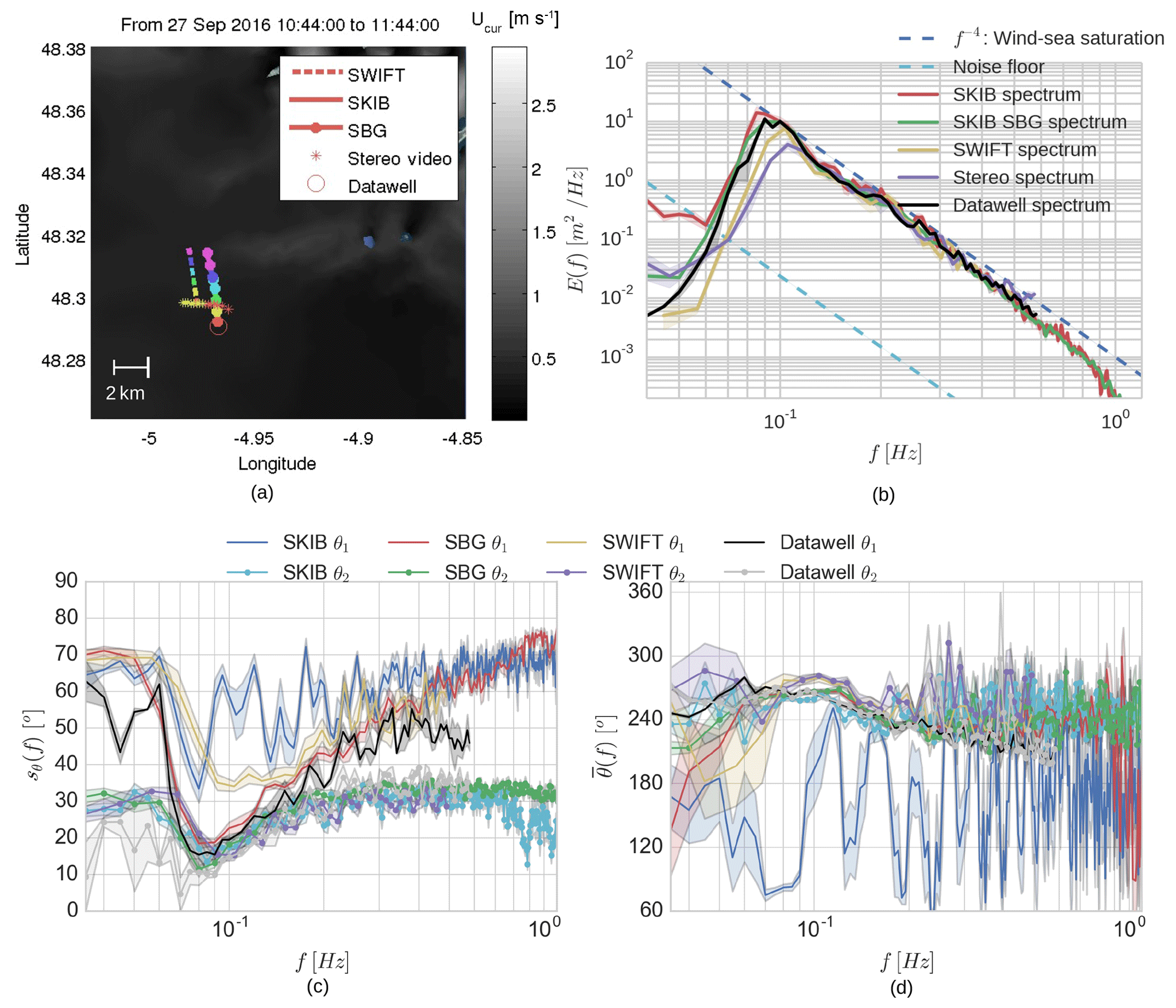
Figure 3 Comparison of wave spectra estimates from SKIB, SWIFT, Datawell and stereo video. (a) Wave sensor path, with the colors representing 10 min displacement, starting in red: (b) E(f) sea surface variance spectral density; (c) s_θ(f) directional spreading from first- and second-order angular moments (θ₁ and θ₂); (d) $\stackrel{\mathrm{‾}}{\mathit{\theta }}\left(f\right)$ frequency-dependent mean wave direction from first- and second-order angular moments (θ₁ and θ₂). The shadow in the lines represent the error for a 95 % confidence interval.

The stereo-video system is the same as used by Leckler et al. (2015), based on a pair of synchronized video cameras (2048×2456 pixels) BM-500GE JAI, mounted with wide-angle lenses. Here the system was installed at the bow of R/V Thalia, a 24.5 m ship of the French coastal oceanographic fleet (Fig. 2d). The cameras are located approximately 7 m above the sea surface, and an Ellipse-D inertial measurement unit is fixed on the bar joining the cameras to correct for ship motion with 0.2^∘ accuracy on all rotation angles. The video processing follows Benetazzo et al. (2016). The only difference in the present case is that the mean surface plane correction, which was used for deployment from fixed platforms, is replaced by an optimization of the rotation matrix given by an SBG motion package mounted with the cameras. The resulting surface elevation maps $\mathit{\zeta }(x,y,t)$ acquired over 30 min records at 12 Hz are gridded in a 10 by 10 m square surface with 0.1 m resolution. This square moves with the mean velocity U_m, relative to the solid Earth, as given by the GPS data. The 3-D spectrum $E(k_x,k_y,f)$ was obtained after applying a Hann window in all three dimensions to the elevation maps over time intervals of 85.33 s (1024 frames), with 50 % overlapping as well. As a result, the energy over frequency and wavenumber are in a reference frame moving at the speed U_m, and the measured radian frequency of the waves σ_m must be corrected by the mean ship velocity (U_m) over each time window. So the absolute frequency in an Earth reference frame is $\mathit{\omega }={\mathit{\sigma }}_{\mathrm{m}}-\mathit{k}\cdot {\mathit{U}}_{\mathrm{m}}$. This procedure is particularly prone to errors for wave components longer than 20 m, which are not resolved in the field of view. These longer components can be treated separately using a slope array estimation of the directional spectrum (Leckler et al., 2015), but we focus here on the short waves. The stereo heave frequency spectrum E(f) is obtained by integration over wavenumbers, and it is expressed in terms of the absolute frequency f_a, with $\mathit{\omega }=\mathrm{2}\mathit{\pi }{f}_{\mathrm{a}}=\mathit{\sigma }+\mathit{k}\cdot \mathit{U}$, where U is a current field that can be estimated using the drifting buoys.

A comparison of the different sensors at the same sea state conditions is shown in Fig. 3. For this comparison the records from each sensor were synchronized over 10 min intervals and averaged over the 30 min of the Waverider records and an integration interval from 0.06 to 0.58 Hz. Figure 3a shows the buoys' drift trajectories for the 1 h of the acquisition, with one color symbol every 10 min and the track of R/V Thalia. The stereo-video record is 20 min, starting at the same time as SKIB and SWIFT acquisitions. The Waverider data correspond to two acquisition of 28 min each, ending at 10:30 and 11:00 UTC.

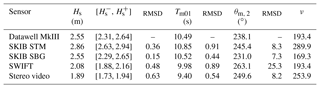
Table 1 Comparison of wave parameters, significant waves height (H_s), mean absolute wave period (T_m01) and mean wave direction (θ_m,2). The root mean square difference between Waverider and other sensors is given in a second column for each variable. [$H_{\mathrm{s}}^{-}$, $H_{\mathrm{s}}^{+}$] represents the maximum and minimum limits for 95 % H_s confidence interval, considering a chi square distribution (Young, 1995) for two perfect devices measuring the same random wave field.

A closer look at the heave spectra (Fig. 3b) shows a good correspondence between Datawell Waverider and SKIB buoys at the peak of the spectrum. The main source of error in the SWIFT data, around the peak of the spectrum, was associated with a high-pass filter applied to the IMU acceleration before each time integration. This part of the SWIFT processing, to obtain E(f), was optimized by Thomson et al. (2016) to reduce the low-frequency noise and to have best agreement with a Datawell Waverider at Ocean Station Papa. This was obtained from the double time integration of the IMU acceleration, with a high-pass filter at each integration, to reconstruct a wave-resolved time series of sea surface elevations. This generally improves the estimation of the spectrum for f>0.1 Hz, but it reduces the level of lower frequencies (as it is also observed in Fig. 3b).

For the SKIBs we have not filtered the acceleration data and the E(f) was directly obtained from the double time integration of the accelerometer data. Other differences are found for the main direction (Fig. 3d), which is better retrieved with the SBG IMU. The main benefit of the SBG IMU is the reduction of the noise floor at low frequencies compared to an estimation of the motion from GPS alone. This is most important for swells of long periods and low heights but not critical for our investigation of wind seas interacting with currents.

Figure 3c and d present the estimates of s_θ and $\stackrel{\mathrm{‾}}{\mathit{\theta }}$ based on the first- and second-order angular moments. We see a significant difference in the wave spread and mean direction estimates, especially in the first-order estimation (s_θ1 and $\stackrel{\mathrm{‾}}{{\mathit{\theta }}_{\mathrm{1}}}$). This occurs because the accelerometer is not internally synchronized with the GPS and because they have different characteristics errors. The second-order moment depends only on the horizontal displacements while the first-order moment depends on both horizontal and vertical displacements. So, the second-order moments are more accurate because there is no cross product between different sensors. Although there are differences, the results suggest that the usage of the combination of GPS drifter displacement and vertical acceleration produces a good estimation of the spectrum directionality. These results are particularly important, as the drifter was not equipped with a compass and only used a low-cost GPS receiver. Because the GPS acquisition was limited to 1 Hz in the SKIB with STM accelerometer, the directional analyses are limited to 0.5 Hz (and 0.8 Hz for SBG, which uses only accelerometer data).

A comparison of the different sensors in terms of the usual sea state parameters is shown in Table 1, with the significant wave height H_s, mean wave period T_m0,1 and peak wave period T_p. Since the only reliable directions are provided by the GPS data alone, we define the peak wave direction D_p and the mean wave direction (θ_m,2) from the second moments as ${\mathit{\theta }}_{\mathrm{m},\mathrm{2}}=\mathrm{0.5}{\tan }^{-\mathrm{1}}(B_{\mathrm{2}}/A_{\mathrm{2}})$ with

$$\begin{array}{}\text{(8)}& {\displaystyle }& {\displaystyle }{A}_{\mathrm{2}}=\int E\left(f\right)a_{\mathrm{2}}\left(f\right)\mathrm{d}f,\text{(9)}& {\displaystyle }& {\displaystyle }{B}_{\mathrm{2}}=\int E\left(f\right)b_{\mathrm{2}}\left(f\right)\mathrm{d}f.\end{array}$$

As reported in Table 1, SKIB results generally agree on H_s, T_m01 and mean directions, with confidence intervals for H_s overlapping with the reference Waverider buoy.

The largest differences are between the SKIB STM and SWIFT buoys and are associated with the filtering of low-frequency content in the SWIFT processing chain (Fig. 3b) and unfiltered low-frequency noise in the SKIB STM. However, for frequencies from 0.1 to 0.5 Hz, the spectra are consistent with the stereo video and Datawell Waverider data. At higher frequencies, for which we do not have other validation data, the power spectra result follows the same trend and appears realistic up to at least 0.8 Hz, consistent with laboratory tests (Thomas, 2015).

In order to validate the SKIB buoys in different sea state conditions, other deployments were performed next to the buoy 62069: one on 5 August 2015 and another four between 21 and 27 September of 2016. For the 2016 experiment, we used two SKIB buoys equipped with SBG IMU and two others with the STM accelerometer. For the 2015 experiment we had only one buoy equipped with the STM accelerometer. Results for integral parameters are presented in Fig. 4, and a selection of two spectra with different shapes is shown in Fig. 5.

For most sea states H_s and D_p are measured correctly (Fig. 4a and d), with RMSE around 0.3 m and 5.3^∘, respectively. As expected, the SKIB SBG agrees best with the Waverider for all the analyzed parameters, and the regression lines for the SBG data (Fig. 4) are closer to the ideal correlation line (gray dashed lines Fig. 4) than those from the SKIB STM data. In general, the STM accelerometer has more energy at the lower frequencies and this can produce overestimations in H_s and T_m01 measurements.

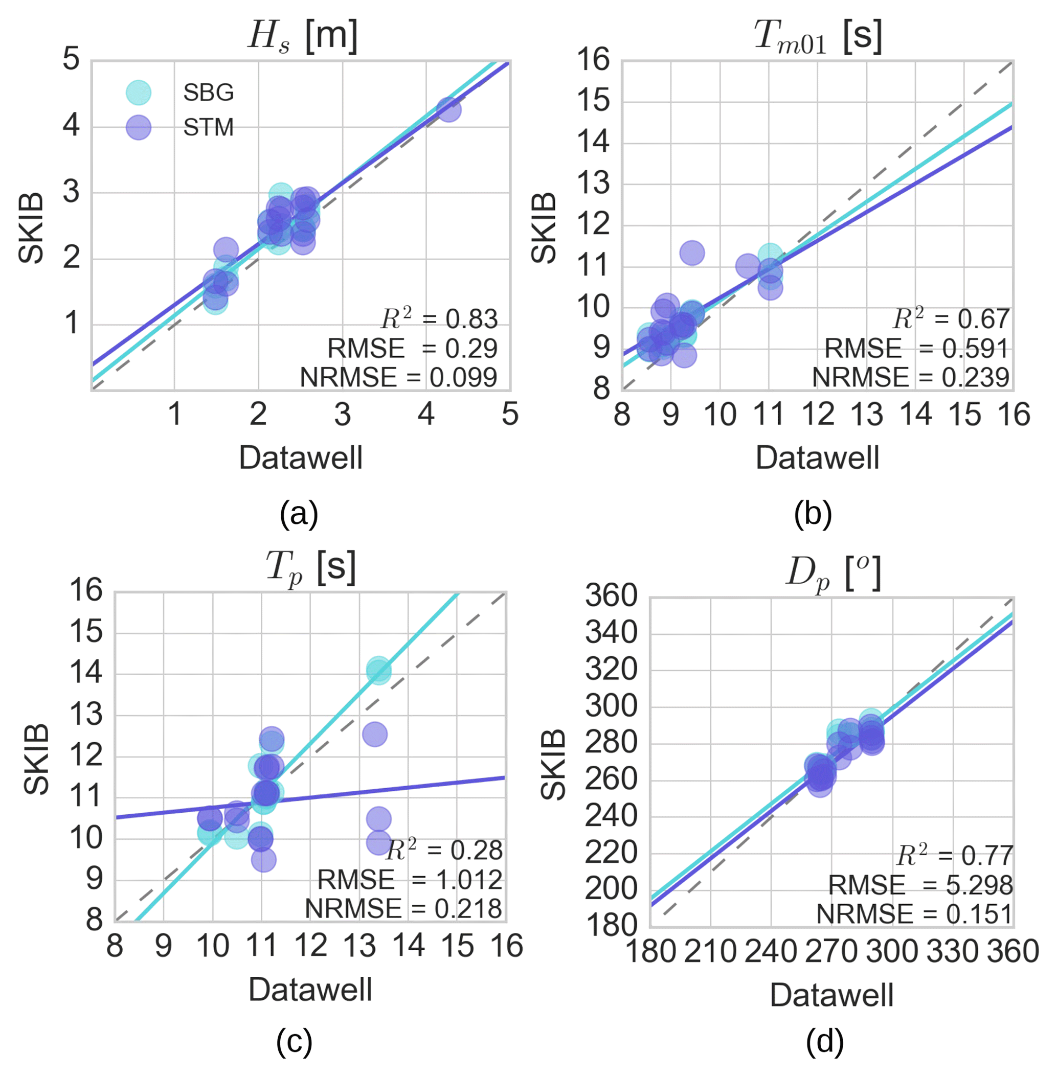
Figure 4 Comparison of the integrated wave parameter estimates from Datawell and SKIB with SBG (IMU sensor) and STM (accelerometer). (a) Significant wave height (H_s). (b) Mean wave period (T_m01). (c) Peak wave period (T_p) and (d) peak direction (D_p) for a frequency interval between 0.06 and 0.6 Hz. The regression lines are computed independently for the SBG and STM data set. The gray dashed line represent the ideal correlation regression line, and the statistics coefficients written in the figures are computed considering both data sets from SBG and STM. The statistical parameters are the Pearson's coefficient of determination R², the root mean square error (RMSE) and the normalized root mean square error (NRMSE).

These errors are confined to frequencies below 0.12 Hz. The main difference between the SKIB and Datawell Waverider was found at the peak wave period (T_p, Fig. 4c). Higher errors in the identification of the peak frequency are expected a priori as the buoys present different spectral resolutions and different numbers of degrees of freedom (Young, 1995). Again the SKIB SBG performs better than SKIB STM.

The buoy's low-frequency noise varies according to the sea state conditions. The errors associated with the low-frequency limit and at the spectrum peak are illustrated in Fig. 5.

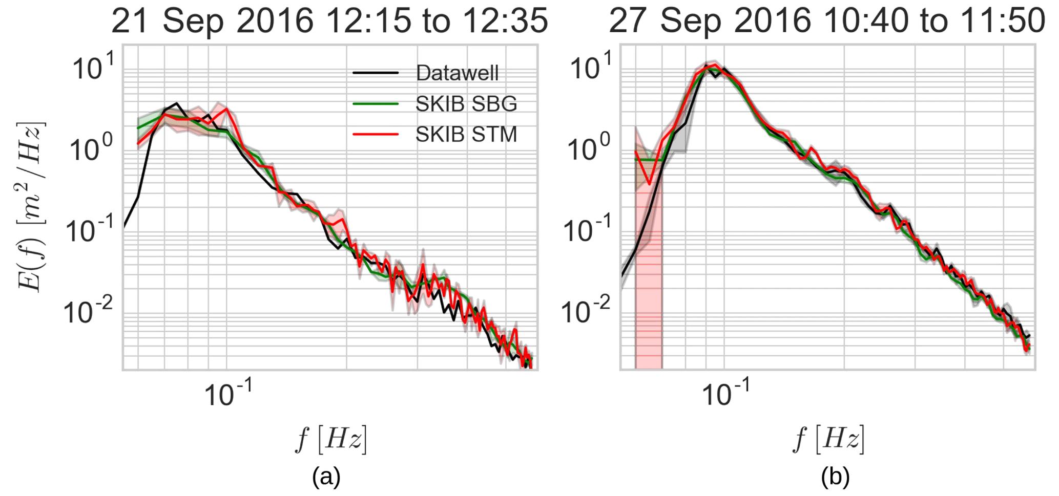
Figure 5 Comparison of Datawell and SKIB with SBG and STM for the sea surface variance spectral density E(f) for two different field measurements around the Datawell Waverider buoy “Pierres Noires” (with World Meteorological Organization number 62069).

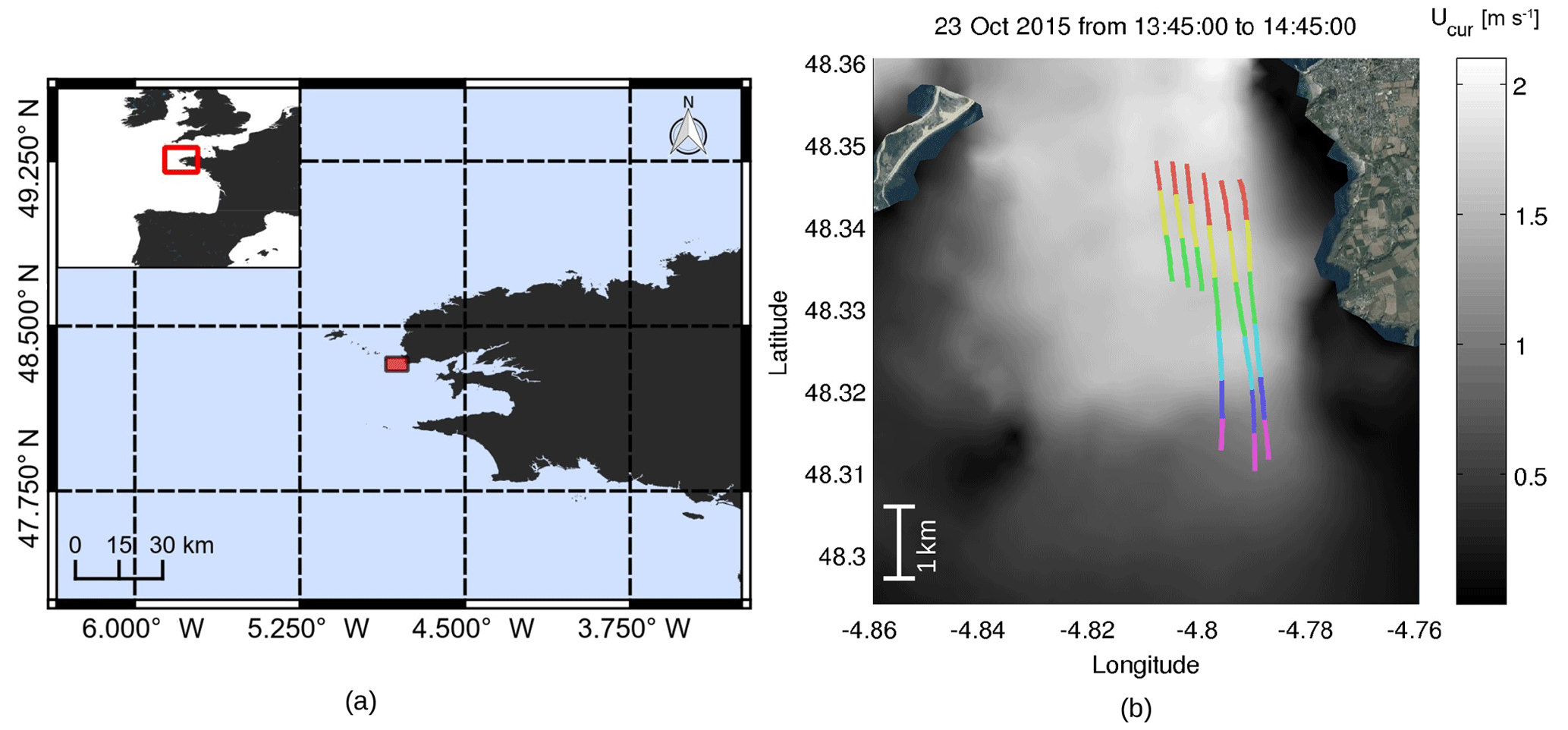
Figure 6 Study field location and local experimental conditions. (a) Chenal du Four location. (b) Local current condition and drifter path. The current field shown here comes from a barotropic model simulation at 250 m resolution (Lazure and Dumas, 2008; Pineau-Guillou, 2013). Colored lines shows the 10 min SKIB displacement over the current gradient on 23 October 2015, 14:40 UTC.

In most sea states analyzed here, the SKIB buoy correctly measured the sea state condition at frequencies higher than 0.07 Hz. In terms of H_s, the instrument usually presents a root mean square error within the statistical uncertainty expected for two perfect devices measuring the same random wave field (Young, 1995). However, because of a significant low-frequency noise in SKIB STM we reduced the integration interval for this buoy. The low-frequency noise was reduced by using the SBG IMU, which presented the best performance among the sensors tested here. In summary, we had a good performance of SKIB for f>0.07 Hz, which makes it appropriate to use in the investigation of young wind waves interacting with currents.

4 Wave evolution in current gradients

Wave properties are largely defined by the wind field and the geometry of the basin in which they develop, but currents can introduce large variations, particularly on small scales (Ardhuin et al., 2017; Masson, 1996; Phillips, 1984). Current effects are generally strongest for the shortest wave components due to a larger ratio of current speed to phase speed and can enhance the probability of wave breaking (Chawla and Kirby, 2002; Zippel and Thomson, 2017).

Here we illustrate the capabilities of SKIB drifters with a deployment through a current gradient that opposes the waves, following the method of Pearman et al. (2014). We deployed buoys in the current upstream of a large gradient area and recorded the evolution of the wave field as the buoys drifted across the current gradient.

The selected area for this study is at the southern end of the Chenal du Four, a passage oriented north–south surrounded by shallow rocks, with Beniguet island to the west and the mainland to the east (see Fig. 6). The water depth in this region ranges from 10 to 13 m relative to chart datum, and increases to 25 m at the southern end near 48.32^∘ N. At the time of our measurements, the water depth was the depth relative to chart datum plus 6 m. The tidal flow in this area is stronger in the shallower part of the channel, resulting in a current gradient at the channel mouth that often enhances wave breaking and can lead to hazardous navigation conditions.

On 23 October 2015 from 13:40 to 14:40 UTC, six drifters buoys were deployed from a small boat (see Fig. 2a).

Winds were approximately 6.2 m s⁻¹ from the south, blowing against a tidal current of approximately 1.4 m s⁻¹ (see Fig. 7). The offshore wave conditions, as recorded by the Waverider buoy, included a 0.9 m swell with a peak period of 13 s coming from west–northwest and a 1.2 m wind sea. The location of our measurements is well sheltered from this west–northwest swell, and the swell heights tend to increase as the buoys drift away from Chanel du Four. Figure 7 presents the mean current velocity estimated from the successive GPS positions for all buoys and each of the 10 min records over which wave spectra are estimated. After increasing from 1.3 to 1.4 m s⁻¹, the current drops to 0.9 m s⁻¹ over the deeper region. As the waves travel against the current, they first experience the increase in the adverse current from 0.9 to 1.4 m s⁻¹.

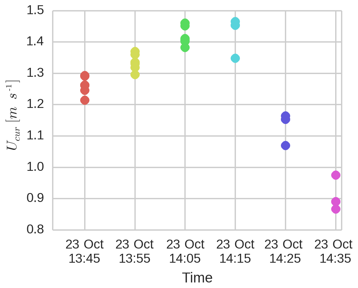
Figure 7 Evolution of the current speed during the drift of the buoys. For each time segment, each dot represents a single buoy.

The corresponding wave spectra are shown in Fig. 8. There is little variation in the mean direction and directional spread (not shown).

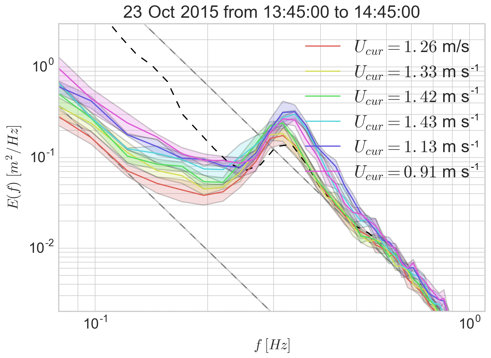
Figure 8 Variance spectral density evolution over time; 10 min Fourier transform from 23 October 2015 13:40 to 14:40 UTC. The gray dashed lines shows the wind-sea saturation f⁻⁴ and noise floor at E(f)f⁴ limits for the first 10 min of acquisition. The color of the lines follows the buoys' displacement as in Fig. 6. The solid lines shows the spatial mean of the spectral density measured in f_r during each 10 min acquisition. The lines' shadow represent the 99 % confidence interval. The dashed dark line is the spectral density measured by Pierre Noires Datawell Waverider buoy at a nearby offshore location, outside the current region.

The increase in energy at low frequencies is mostly due to the buoys drifting to more exposed areas in the presence of a swell. The effect of the current on the shape of the wind waves is analyzed using the nondimensional saturation spectrum B, following Phillips (1984). With a velocity increase Δ_U=0.3 m s⁻¹ over a 1 km scale, we measure an increase in the saturation level at frequencies from 0.35 to 0.5 Hz that does not exceed 50 %. The following reduction in wave energy is more pronounced over the 3 km where the current slows down.

Figure 9 shows that the saturation level increases when waves face an accelerating and opposing current. This is similar to the cases studied in Zippel and Thomson (2017), from the Columbia River, in which opposing currents increase the steepness locally (without gradient analysis). In the final portion of the trajectories, the current speed decreases and the saturation relaxes to a lower value.

Given the complex interaction of wave generation by the wind, wave dissipation by breaking and nonlinear evolution, there are no simple theoretical results to interpret our observations. Starting from a dynamical balance in the absence of currents, Phillips (1984) provides an analysis of the current effect as a deviation of the wave spectrum from a near-equilibrium state, assuming that the wind forcing is proportional to B and a dissipation rate that is proportional to Bⁿ with n≃3. For a scale of current variation L, he finds that the maximum value of B is

$$\begin{array}{}\text{(10)}& {\displaystyle }{B}_{max}=B_{\mathrm{0}}{\left[\mathrm{1}+\mathrm{18}{\mathrm{\Delta }}_U/\left(cS\right)\right]}^{[\mathrm{1}/(n-\mathrm{1}\left)\right]},\end{array}$$

where B₀ is the equilibrium level of the saturation outside of the current gradient. In this expression c is the phase speed and S is the scale of current variation normalized by the wind stress $S=L{k}^{\mathrm{2}}{C}_d{U}_{\mathrm{10}}^{\mathrm{2}}/\left(\mathrm{2}\mathit{\pi }g\right)$. In our case, taking L=1.5 km gives S=0.93 for f_r=0.5 Hz. With the same parameters, Δ_U=0.4 m s⁻¹ and n=3 in Eq. (7) gives $B_{max}=\mathrm{1.8}{B}_{\mathrm{0}}$. If n is reduced to 2, $B_{max}/B_{\mathrm{0}}$ is as large as 3.4 and diverges as n goes to 1. In other words, the dissipation rate must be a very steep function of B in order to absorb the wind forcing energy that converges into the small region of the current gradient. The limited increase in B in our data supports n>2. With n=3, Eq. (7) gives a reduction in $B_{max}/B_{\mathrm{0}}$ from 1.8 at 0.5 Hz to 1.25 at 0.8 Hz, which is consistent with the weaker ratio found for the higher frequencies in Fig. 9.

For example, a current speed of 1.6 m s⁻¹ corresponds to blocking conditions for waves with periods shorter than 2 s, which have a group speed slower than 1.6 m s⁻¹, and these short waves should be strongly attenuated in a fixed reference frame. However, our measurements are in a reference frame moving with the current, in which the waves, even those with periods shorter than 2 s, are propagating past the drifting buoys. At frequencies above 0.5 Hz, the intrinsic group speed is less than 1.6 m s⁻¹ and waves must be generated by the local wind and cannot propagate from the south. Our data are consistent with n=3, as used in Banner et al. (2000) and Ardhuin et al. (2010).

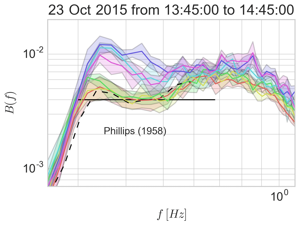
Figure 9 Saturation of the spectral density. Time evolution over 10 min Fourier transform from 23 October 2015 13:40 to 14:40 UTC. The colored lines follow the buoys' displacement as in Fig. 8. The solid lines show the spatial mean of the spectral density measured during each 10 min acquisition. The lines' shadow represents the 99 % confidence interval. The dashed black line is the saturation measured at an offshore location by the Pierre Noires Datawell buoy.

5 Summary and conclusion

The surface kinematics buoy (SKIB) is a new drifter that has been designed for the investigation of wave–current interactions, including relatively short waves from 0.07 Hz and up to 1 Hz in frequency. Here we mostly used the heave data from the accelerometer that was first validated by comparing it to the reference Datawell Waverider buoy up to 0.6 Hz. Typical costs for the electronics are around EUR 1100, with an additional EUR 1100 for the hull, which could be reduced by using plastics instead of our glass sphere. The combined analysis with the vertical acceleration and buoy velocity from the instrument GPS allowed us to measure the directional properties of the wave spectrum without using an internal compass, simplifying the equipment design and reducing the costs. Still, the combination of the GPS velocity and accelerometer posed particular problems, and only the parameters θ₂ and s_θ2 obtained from the GPS velocity appear reliable.

For cases in which the steepness of the waves of interest is very small, we replaced the cheap STM accelerometer by an SBG Ellipse-N inertial navigation unit. This SKIB SGB model performs better, both for the heave spectrum and for the directional parameters derived from first moments (θ₁ and s_θ1). This model was used by Sutherland and Dumont (2018) for the investigation of wave propagation in sea ice.

The capabilities of the new drifters were illustrated here by measuring the variation in wave properties across a current gradient that was relatively uniform and along the propagation direction. Such measurements are important for testing existing theories for wave dissipation, such as proposed by Phillips (1984) and now widely used in numerical wave models (Ardhuin et al., 2010). In particular, the frequency-dependent saturation level is found to respond to current gradients in a way that is consistent with the proposition by Phillips (1984) of a nonlinear dissipation rate. We expect further applications to the investigation of small-scale gradients in wave heights and mean square slopes in the presence of current gradients.