the Creative Commons Attribution 4.0 License.
the Creative Commons Attribution 4.0 License.
 | 25 Sep 2018
Recent updates to the Copernicus Marine Service global ocean monitoring and forecasting real-time 1∕12° high-resolution system
Jean-Michel Lellouche
Eric Greiner
Olivier Le Galloudec
Gilles Garric
Charly Regnier
Marie Drevillon
Mounir Benkiran
Charles-Emmanuel Testut
Romain Bourdalle-Badie
Florent Gasparin
Olga Hernandez
Bruno Levier
Yann Drillet
Elisabeth Remy
Pierre-Yves Le Traon
Since 19 October 2016, and in the framework of Copernicus Marine Environment Monitoring Service (CMEMS), Mercator Ocean has delivered real-time daily services (weekly analyses and daily 10-day forecasts) with a new global 1∕12∘ high-resolution (eddy-resolving) monitoring and forecasting system. The model component is the NEMO platform driven at the surface by the IFS ECMWF atmospheric analyses and forecasts. Observations are assimilated by means of a reduced-order Kalman filter with a three-dimensional multivariate modal decomposition of the background error. Along-track altimeter data, satellite sea surface temperature, sea ice concentration, and in situ temperature and salinity vertical profiles are jointly assimilated to estimate the initial conditions for numerical ocean forecasting. A 3D-VAR scheme provides a correction for the slowly evolving large-scale biases in temperature and salinity.
This paper describes the recent updates applied to the system and discusses the importance of fine tuning an ocean monitoring and forecasting system. It details more particularly the impact of the initialization, the correction of precipitation, the assimilation of climatological temperature and salinity in the deep ocean, the construction of the background error covariance and the adaptive tuning of observation error on increasing the realism of the analysis and forecasts.
The scientific assessment of the ocean estimations are illustrated with diagnostics over some particular years, assorted with time series over the time period 2007–2016. The overall impact of the integration of all updates on the product quality is also discussed, highlighting a gain in performance and reliability of the current global monitoring and forecasting system compared to its previous version.
- Article
(10026 KB) - Full-text XML
- BibTeX
- EndNote


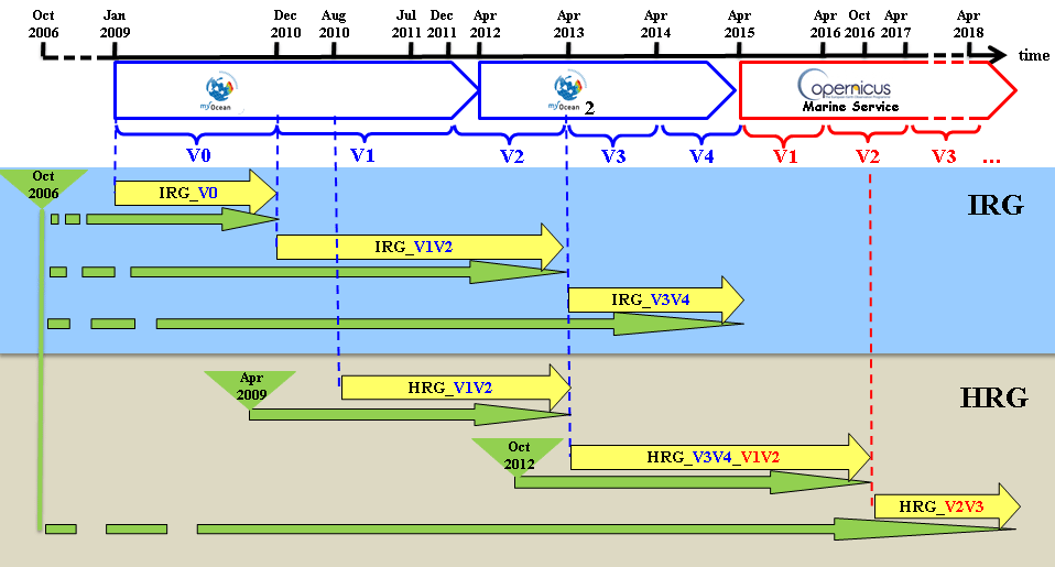
Figure 1Timeline of the Mercator Ocean global analysis and forecasting systems for the various milestones (from V0 to V4) of the past MyOcean project and for milestones V1, V2 and V3 of the current CMEMS. Real-time productions are in yellow with the reference of the Mercator Ocean system. Available Mercator Ocean simulations are in green, including the catchup to real time. Global intermediate-resolution (high-resolution) systems at 1∕4∘ (1∕12∘) are referred to as IRG (HRG). Milestones are written in blue for the MyOcean project and in red for CMEMS.
Table 1Specifics of the Mercator Ocean IRG systems. In italic are the major upgrades with respect to the previous version. Available and operational production periods are described in Fig. 1.
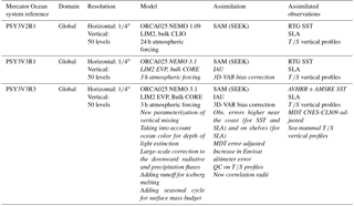
Table 2Specifics of the Mercator Ocean HRG systems. In italic are the major upgrades with respect to the previous version. Available and operational production periods are described in Fig. 1.
Mercator Ocean monitoring and forecasting systems have been routinely operated in real time since early 2001. They have been regularly upgraded by increasing complexity, expanding the geographical coverage from regional to global, and improving models and assimilation schemes (Brasseur et al., 2006; Lellouche et al., 2013).
Mercator Ocean, which had primary responsibility for the global ocean forecasts of the MyOcean and MyOcean2 projects since January 2009, developed several versions of its monitoring and forecasting systems for the various milestones (from V0 to V4) of the MyOcean project and, more recently, for milestones V1, V2 and V3 of the Copernicus Marine Environment Monitoring Service (CMEMS) as part of the European Earth observation program Copernicus (http://marine.copernicus.eu, last access: 20 September 2018) (see Fig. 1). Since May 2015, in the context of CMEMS, research and development activities have been conducted to improve the real-time 1∕12∘ high-resolution (eddy-resolving) global analysis and forecasting system. Since 19 October 2016, Mercator Ocean has delivered real-time daily services (weekly analyses and daily 10-day forecasts) with a new global 1∕12∘ system PSY4V3R1 (hereafter PSY4V3; see Fig. 1). Note that PSY4V3 will be the system for the CMEMS V4 milestone. The main differences and links between the various versions of the Mercator Ocean systems in the framework of the past MyOcean project and current CMEMS are summarized in Tables 1 and 2 for intermediate-resolution 1∕4∘ global configuration (hereafter IRG) and high-resolution 1∕12∘ global configuration (hereafter HRG) systems, respectively.
These systems are intensively used in four main areas of application: (i) maritime safety, (ii) marine resources management, (iii) coastal and marine environment, and (iv) weather, climate and seasonal forecasting (http://marine.copernicus.eu/markets/use-cases, last access: 20 September 2018). As described in Lellouche et al. (2013), the evaluation of such systems includes routine verification against assimilated and independent in situ and satellite observations, as well as a careful check of many physical processes (e.g., mixed layer depth evaluation as shown in Drillet et al., 2014). Scientific studies brought precious additional evaluation feedbacks (Juza et al., 2015; Smith et al., 2016; Estournel et al., 2016). Finally, several studies showed the added value of surface current analyses provided by these systems for drift applications (Scott et al., 2012; Drevillon et al., 2013).
In the system PSY4V3, the ocean–sea ice model and the assimilation scheme benefit from the following main updates: atmospheric forcing fields are corrected at large scale with satellite data; freshwater runoff from ice sheet melting is added to river runoffs; a time-varying global average steric effect is added to the model sea level; the last version of GOCE geoid observations are taken into account in the mean dynamic topography used for sea level anomaly assimilation; adaptive tuning is used on some of the observational errors; a dynamic height criteria is added to the quality control of the assimilated temperature and salinity vertical profiles; satellite sea ice concentrations are assimilated; and climatological temperature and salinity in the deep ocean are assimilated below 2000 m to prevent drifts in those very sparsely observed depths.
The impact of all these updates can be evaluated separately thanks to an incremental implementation taking advantage of Mercator Ocean's specific hierarchy of system configurations running with an identical setup. To this aim, short simulations (from 1 year to a few years) were performed by adding from one simulation to another one upgrade at a time using the IRG configuration or some high-resolution regional configuration.
The system PSY4V3 was run over the October 2006–October 2016 period to catch up to real time, assimilating the “reprocessed” observations (along-track altimeter, satellite sea surface temperature, sea ice concentration, and in situ temperature and salinity vertical profiles) available at that time and the so-called “near-real-time” observations otherwise. Moreover, in the development phase of the operational system PSY4V3, it was decided to systematically perform two other twin numerical simulations over the same time period, maintaining the same ocean model tunings but varying the complexity and the level of data assimilation. The first one is a free simulation (without any data assimilation) and the second one only benefits from temperature and salinity large-scale bias correction using in situ observed temperature and salinity vertical profiles. Intercomparisons between the three simulations were then conducted in order to better analyze and try to quantify the impact of some component of the assimilation system. These three versions of the system have been used to quantify the impact of some updates.
In a previous paper (Lellouche et al., 2013), the main results of the scientific evaluation of MyOcean global monitoring and forecasting systems at Mercator Ocean showed how refinements or adjustments to the system impacted the quality of ocean analyses and forecasts. The primary objective of this paper is to describe the recent updates applied to the system PSY4V3 and show the highest impact on the product quality. Updates resulting from routine system improvements are not separately illustrated and discussed (bathymetry, runoffs, assimilated databases, mean dynamic topography, etc.). So, particular focus was given to the initialization, correction of precipitation, assimilation of climatological temperature and salinity in the deep ocean, construction of background error covariance and the adaptive tuning of observation error. Another objective of this paper is to present a first-level evaluation of the system. The purpose here is not to perform an exhaustive validation but only to check the global behavior of the system compared to assimilated quantities or independent observations. Thus, an assessment of the hindcast (2007–2016) quality is conducted and improvements with respect to the previous system are highlighted in order to show the level of performance and the reliability of the system PSY4V3. A complementary study is aimed at demonstrating the scientific value of PSY4V3 for resolving oceanic variability at regional and global scale (Gasparin et al., 2018). Lastly, several scientific studies have investigated local ocean processes by comparing the PSY4V3 system with independent observation campaigns (Koenig et al., 2017; Artana et al., 2018). This reinforces the system PSY4V3 evaluation effort.
This paper is organized as follows. The main characteristics of the system PSY4V3 and details concerning the updates are described in Sect. 2. The impact of some sensitive upgrades is shown in Sect. 3. Results of the scientific evaluation, including some comparisons with independent observations, are given in Sect. 4. Section 5 contains a summary of the scientific assessment and a discussion of future improvements for the next version of the global high-resolution system.
This section contains the main characteristics of the CMEMS system PSY4V3 and details the last updates to the system compared to the previous system PSY4V2R2 (hereafter PSY4V2; see Fig. 1 and Table 2). A detailed description of some sensitive updates is provided in Sect. 3.
2.1 Physical model and latest updates
The system PSY4V3 uses version 3.1 of the NEMO ocean model (Madec et al., 2008). This NEMO version has been available for a few years and has already been used in the previous system PSY4V2. This was the available stable version of the code when we started the development of the system PSY4V3 a few years ago. Note that by using this version of the code, we do not access the better algorithms and more sophisticated parameterizations present in the version 3.6, which is the latest official release of NEMO. The physical configuration is based on the tripolar ORCA12 grid type (Madec and Imbard, 1996) with a horizontal resolution of 9 km at the Equator, 7 km at Cape Hatteras (midlatitudes) and 2 km toward the Ross and Weddell seas. Z coordinates are used on the vertical; the 50-level vertical discretization retained for this system has a decreasing resolution from 1 m at the surface to 450 m at the bottom and 22 levels within the upper 100 m. A “partial cell” parameterization (Adcroft et al., 1997) is chosen for a better representation of the topographic floor (Barnier et al., 2006) and the momentum advection term is computed with the energy- and enstrophy-conserving scheme proposed by Arakawa and Lamb (1981). The advection of the tracers (temperature and salinity) is computed with a total variance diminishing (TVD) advection scheme (Levy et al., 2001; Cravatte et al., 2007). We use a free surface formulation. External gravity waves are filtered out using the Roullet and Madec (2000) approach. A Laplacian lateral isopycnal diffusion on tracers (100 m2 s−1) and a horizontal biharmonic viscosity for momentum ( m4 s−1) are used. In addition, the vertical mixing is parameterized according to a turbulent closure model (order 1.5) adapted by Blanke and Delecluse (1993). The lateral friction condition is a partial-slip condition with a regionalization of a no-slip condition (over the Mediterranean Sea), and the elastic–viscous–plastic rheology formulation for the LIM2 ice model (Fichefet and Maqueda, 1997) has been activated (Hunke and Dukowicz, 1997). Instead of being constant, the depth of light extinction is separated in red–green–blue bands depending on the chlorophyll data distribution from mean monthly SeaWIFS climatology (Lengaigne et al., 2007). The bathymetry used in the system is a combination of interpolated ETOPO1 (Amante and Eakins, 2009) and GEBCO8 (Becker et al., 2009) databases. ETOPO1 datasets are used in regions deeper than 300 m and GEBCO8 is used in regions shallower than 200 m with a linear interpolation in the 200–300 m layer. Internal-tide-driven mixing is parameterized following Koch-Larrouy et al. (2008) for tidal mixing in the Indonesian seas, as the system does not explicitly represent the tides. The atmospheric field forcings for the ocean model are taken from the ECMWF (European Centre for Medium-Range Weather Forecasts) IFS (Integrated Forecast System). A 3 h sampling is used to reproduce the diurnal cycle. Momentum and heat turbulent surface fluxes are computed from the Large and Yeager (2009) bulk formulae using the following set of atmospheric variables: surface air temperature and surface humidity at a height of 2 m and mean sea level pressure and wind at a height of 10 m. Downward longwave and shortwave radiative fluxes and rainfall (solid + liquid) fluxes are also used in the surface heat and freshwater budgets. Compared to the previous HRG system PSY4V2, the following updates were done on the model part (see Table 2).
-
The bathymetry used in the system benefited from a specific correction in the Indonesian seas inherited from the INDESO system (Tranchant et al., 2016).
-
In order to solve numerical problems induced by the use of z coordinates on the vertical (Willebrand et al., 2001), a relaxation toward the World Ocean Atlas 2013 (version 2) 2005–2012 time period (hereafter WOA13v2, https://data.nodc.noaa.gov/woa/WOA13/DOC/woa13v2_changes.pdf, last access: 20 September 2018) temperature (Locarnini et al., 2013) and salinity (Zweng et al., 2013) climatology has been added at the Gibraltar and Bab-el-Mandeb straits. Indeed, z coordinates, compared to sigma, isopycnal or hybrid coordinates, induce excessive numerical mixing over overflow sills (Winton et al., 1998). For instance, Mediterranean overflow, without any relaxation, would settle at an equilibrium depth of 800 m or so otherwise instead of the 1100 m observed. Sigma coordinates could indeed improve the representation of overflow processes but are likely to induce other problems elsewhere due to sigma gradient pressure error over steep topography or excessive diapycnal mixing in the interior (Marchesiello et al., 2009). For Gibraltar (and Bab-el-Mandeb), the relaxation area is centered at 8∘ W, 35∘ N (and 46∘ E, 12∘ N). At the center the relaxation time is 10 days (50 days). This time is increased up to infinity 4∘ (5∘) away from the center. The relaxation is not constant over the vertical. It is only applied below 500 m and it is increased linearly between 500 and 700 m. Between 700 m and the bottom of the ocean the coefficient value is unchanged.
-
Surface wind stress computation should in principle consider wind speed relative to the surface ocean currents (Bidlot, 2012; Renault et al., 2016). However, this statement applies to a fully coupled ocean–atmosphere system, which is not the case for the present system PSY4V3. Based on sensitivity experiments and following the results obtained by Bidlot (2012), we pragmatically consider only 50 % of the surface model currents in the wind stress computation.
-
The monthly runoff climatology is built with data on coastal runoffs and 100 major rivers from the Dai et al. (2009) database (instead of Dai and Trenberth, 2002, for the system PSY4V2). This database uses new data, mostly from recent years, and streamflow simulated by the Community Land Model version 3 (CLM3) to fill the gaps, in all lands areas except Antarctica and Greenland. In addition, we built mean seasonal freshwater fluxes representing Greenland and Antarctica ice sheet and glacier runoff melting. For this purpose we have distributed the following mean values: 545 Gt yr−1 for Greenland and 2400 Gt yr−1 for Antarctic (corresponding to freshwater fluxes of 1.51 and 6.65 mm yr−1, respectively). These values are in the range of estimations given by the IPCC-AR13 (Church et al., 2013). They have been applied along the Greenland and Antarctica coastlines and over an open ocean domain varying seasonally and defined by the climatological presence of icebergs observed by the Altiberg iceberg database project (Tournadre et al., 2016). Domain covered by giant icebergs from Silva et al. (2006) complements southernmost areas not covered by Altiberg data. One-third of these quantities is applied offshore and two-thirds along the Greenland and Antarctic coastlines. We also used negative variations of water masses estimated from GRACE (Bruinsma et al., 2010) to spatially distribute these runoffs along coastlines.
-
As the Boussinesq approximation is applied to the model equations, thereby conserving the ocean volume and varying its mass, the simulations do not properly directly represent the global mean steric effect on the sea level (Greatbatch, 1994). For improved consistency with assimilated satellite observations of sea level anomalies, which are unfiltered from the global mean steric component, a time-evolving global average steric effect is added to the sea level in the simulation. This global average steric effect has been computed as the difference between two successive daily global mean dynamic heights (vertical integration from the surface to the bottom of the specific volume anomaly).
-
Due to large known biases in precipitation (Stephens et al., 2010; Kidd et al., 2013), a satellite-based large-scale correction of precipitation has been performed, except at high latitudes (poleward of 65∘ N and 60∘ S). This is detailed in Sect. 3.
-
In order to avoid mean sea-surface-height drift due to the large uncertainties in the water budget closure, the following two treatments were applied.
-
The surface freshwater global budget has been set to an imposed seasonal cycle (Chen et al., 2005). Only spatial departures from the mean global budget are kept from the forcing.
-
A trend of 2.2 mm yr−1 has been added to the surface mass budget in order to somewhat represent the recent estimate of the global mass addition to the ocean (from glaciers, land water storage changes, Greenland and Antarctica ice sheet mass loss) (Chambers et al., 2017). This term is implemented as a surface freshwater flux in the open ocean domain teeming with observed icebergs.
-
2.2 Data assimilation and latest updates
The data are assimilated by means of a reduced-order Kalman filter derived from a SEEK filter (Brasseur and Verron, 2006), with a three-dimensional multivariate modal decomposition of the background error and a 7-day assimilation cycle. It includes an adaptive-error estimate and a localization algorithm. This data assimilation system is called SAM (Système d'Assimilation Mercator). The background error covariance is based on the statistics of a collection of three-dimensional ocean state anomalies. The anomalies are computed from a long numerical experiment (2007–2015 9-year period for PSY4V3) with respect to a running mean in order to estimate the 7-day scale error on the ocean state at a given period of the year. A Hanning low-pass filter is used to create the running mean with a cutoff frequency equal to 1∕24 days−1. The background error covariances in SAM rely on a fixed basis, seasonally variable ensemble of anomalies. They also contain the interannual signal from the 9-year simulation. This choice implies that, at each analysis step, a subset of anomalies (250 anomalies) is used to improve the dynamic dependency. A significant number of anomalies are kept from one analysis to the other, thus ensuring error covariance continuity. Currently, the anomalies used in real time come from the set of anomalies computed over the 2007–2015 period with no real-time extension of this set. We therefore make the hypothesis that the set of anomalies computed over a period prior to real time is able to correctly represent the background error covariance over the real-time period. Altimeter data, in situ temperature and salinity vertical profiles, and satellite sea surface temperature and sea ice concentration are jointly assimilated to estimate the initial conditions for numerical ocean forecasting. In addition, a 3D-VAR scheme provides a correction for the slowly evolving large-scale biases in temperature and salinity (Lellouche et al., 2013).
Compared to the previous HRG system PSY4V2, the following updates were done on the data assimilation part (see Table 2).
-
CMEMS satellite near-real-time sea ice concentration OSI SAF (http://marine.copernicus.eu/documents/QUID/CMEMS-OSI-QUID-011-001to007-009to012.pdf, last access: 20 September 2018) is a new observation assimilated into the system PSY4V3. For this, a separate monovariate–monodata analysis is carried out for the ice variables in parallel to that for the ocean. The two analyses are completely independent.
-
CMEMS OSTIA SST (delayed time (reprocessed) until the end of 2006: http://marine.copernicus.eu/documents/QUID/CMEMS-OSI-QUID-010-011.pdf (last access: 20 September 2018), then near real time: http://marine.copernicus.eu/documents/QUID/CMEMS-OSI-QUID-010-001.pdf, last access: 20 September 2018) is assimilated into the system PSY4V3 instead of near-real-time AVHRR SST from NOAA in PSY4V2. Particular attention has been devoted to the computation of the model equivalent. As OSTIA provides the foundation SST (considered nominally at 10 m of depth), the SST model equivalent is performed by calculating the nighttime average of the first level of the model temperature. Moreover, only one SST map is assimilated on the fifth day of the 7-day cycle. Cloudy regions are filled by the analysis performed in the OSTIA product.
-
In addition to the quality control based on temperature and salinity innovation statistics (detection of spikes, large biases) already present in the previous system, a second quality control has been developed and is based on dynamic height innovation statistics (detection of small vertically constant biases). This is detailed in Sect. 2.3.
-
A new hybrid MDT based on the CNES-CLS13 MDT (Rio et al., 2014) with adjustments made using the Mercator GLORYS2V3 (GLobal Ocean ReanalYsis and Simulation, stream 2, version 3) reanalysis and with an improved post-glacial rebound (also called glacial isostatic adjustment) has been used. This new hybrid MDT also takes into account the last version of the GOCE geoid. This replaces the previous hybrid MDT used in the previous system PSY4V2, which was based on the CNES-CLS09 MDT derived from observations (Rio et al., 2011). The new hybrid MDT significantly reduces (not shown) sea level bias (more than 5 cm in some areas) and consequently temperature and salinity in regions where the topography makes the mean sea surface estimation difficult (e.g., Indonesia, Red Sea and Mediterranean Sea).
-
A consistent along-track SLA dataset (http://marine.copernicus.eu/documents/QUID/CMEMS-SL-QUID-008-032-051.pdf, last access: 20 September 2018), with a 20-year altimeter reference period, is assimilated all along the simulation performed with the system PSY4V3. Reprocessed observations are assimilated until the end of August 2015. Near-real-time observations are assimilated afterward.
-
The CORA 4.1 CMEMS in situ reprocessed database (Szekely et al., 2016; http://marine.copernicus.eu/documents/QUID/CMEMS-INS-QUID-013-001b.pdf, last access: 20 September 2018) has been assimilated for the 2006–2013 period. In addition to Argo and other in situ datasets, this database includes temperature and salinity vertical profiles from the sea mammal (elephant seals) database (Roquet et al., 2011) to compensate for the lack of such data at high latitudes. From 2014 to present, the near-real-time CMEMS product (http://marine.copernicus.eu/documents/QUID/CMEMS-INS-QUID-013-030-036.pdf, last access: 20 September 2018) is assimilated.
-
As the prescription of observation errors in the assimilation systems is not sufficiently accurate, adaptive tuning of observation errors for the SLA and SST has been implemented. The method has been adapted from diagnostics proposed by Desroziers et al. (2005) and is detailed in Sect. 3.
-
New three-dimensional observation error files for the assimilation of in situ temperature and salinity data have been recomputed from the MyOcean IRG system PSY3V3R3 (see Fig. 1 and Table 1) using an offline version of the adaptive tuning method mentioned above.
-
A weak constraint towards the WOA13v2 climatology on temperature and salinity in the deep ocean (below 2000 m) has been included in the two components (3D-VAR and SEEK filter) of the assimilation scheme to prevent drifts in temperature and salinity and as a consequence to obtain a better representation of the sea level trend at global scale in the system. The method consists of assimilating vertical climatological profiles of temperature and salinity at large scale and below 2000 m in regions drifting away from the climatological values using a non-Gaussian error at depth. This is detailed in Sect. 3.
-
The time window for the 3D-VAR bias correction was reduced from 3 months to 1 month to obtain a correction that is more in line with the current physics, which is made possible by the good spatial and temporal distribution of the Argo network from 2006.
-
In the previous system PSY4V2, the SSH increment was the sum of barotropic and baroclinic (dynamic) height increments as in Benkiran and Greiner (2008). Dynamic height increment was calculated from the temperature and salinity increments, while the barotropic increment was an output of the analysis. Barotropic height was computed without the wind effect. In the system PSY4V3, we directly use the total SSH increment given by the analysis to take into account, among other things, the wind effect like the hydraulic control near the straits (Song, 2006; Menemenlis et al., 2007).
-
The uncertainties in the MDT estimate and the sparsity of the observation networks (both altimetry and in situ profiles) on the 7-day assimilation window do not allow us to accurately estimate the observed global mean sea level. Moreover, the mean sea level time evolution is the result of an imposed trend for mass inputs (2.2 mm yr−1; see Sect. 2.1) together with a diagnostic steric effect recomputed from model T and S. Therefore, the global mean increment of the total sea surface height is set to zero and the mean sea level is not controlled by data assimilation.
-
The background error covariance matrices needed for data assimilation are defined using anomalies of the different variables coming from a simulation in which only a 3D-VAR large-scale bias correction of T and S has been performed (instead of using a free run as was done in the previous system PSY4V2). This new approach is more consistent because it better mimics the final operational system, which also uses the 3D-VAR bias correction. Moreover, these anomalies, which are inputs of the analysis, are spatially filtered in order to retain only the effective model resolution and in order to avoid injecting noise into the increments. This is detailed in Sect. 3.
2.3 Additional quality controls on in situ observations
To minimize the risk of erroneous observations being assimilated in the model, the system PSY4V3 carries out two successive quality controls (QC1 and QC2) on the assimilated temperature (T) and salinity (S) vertical profiles. These are done in addition to the quality control procedures performed by the data producers. This observation screening is known as background quality control. In both cases (QC1 and QC2), we estimate two parameters, which are the mean and standard deviation of model innovations. These parameters are then used to define space- and season-dependent threshold values that correspond to the mean plus N times the standard deviation. The N parameter is chosen empirically to reach a compromise between rejecting a lot of profiles (if the criterion is too strict) and rejecting on average no more than 1 % of profiles that are contained in the tails of the probability density function of the innovations.
2.3.1 Quality control QC1
The first quality control QC1 has already been described in Lellouche et al. (2013) and can be summarized as follows. An observation is considered suspicious if the two following conditions are both satisfied:
where the spatially and seasonally varying threshold value comes from statistics (mean, standard deviation) computed with the very large number of temperature and salinity innovations collected in the Mercator GLORYS2V1 (GLobal Ocean ReanalYsis and Simulation, stream 2, version 1) reanalysis (1993–2009). The first condition of Eq. (1) is a test on the innovation. It determines whether the innovation is abnormally large, which would most likely be due to an erroneous observation. The second condition avoids rejecting “good” observations (i.e., an observation close to the climatology) even if the innovation is high due to the model background being biased. This first quality control allows for the detection of spikes and large biases.
2.3.2 Quality control QC2
The second quality control QC2 is based on dynamic height innovation (vertical integration from the surface to the bottom) statistics. This quality control allows for the detection of small biases that are present in the whole water column and can thus induce large errors. It basically stipulates that the thermal or haline component of dynamic height innovation (hdyn(innovT) or hdyn(innovS)) cannot exceed some threshold in height (thresholdT for thermal component or thresholdS for haline component). It can be summarized as follows. A vertical profile is rejected if the following condition is satisfied:
where
and dzT is the model layer thickness corresponding to the temperature observation (same for dzS and salinity). These last conditions (Eq. 3) prevent the threshold from being reached too quickly in shallow areas.
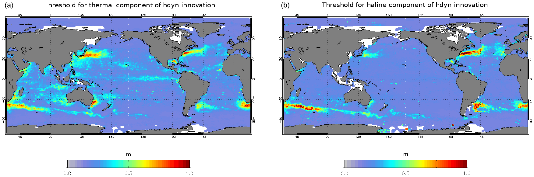
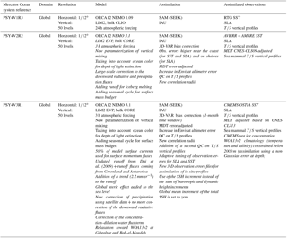
Figure 2Thresholds used for QC2 for the thermal component of dynamical height innovation (a, thresholdT) and for the haline component of dynamical height innovation (b, thresholdS). Units are meters.
The average and standard deviation of the thermal or haline components of dynamical height innovation have been calculated from a global simulation at 1∕4∘, which is a twin simulation of the PSY4V3 one. Note that the simulation at also assimilates the CORA 4.1 CMEMS in situ database. The temperature and salinity threshold two-dimensional fields used by QC2 are then computed as the average plus 6 times the standard deviation of the dynamical height innovations (Fig. 2). With these temperature and salinity thresholds, the system will more easily reject biased salinity profiles in the tropics and biased temperature profiles in strong currents.
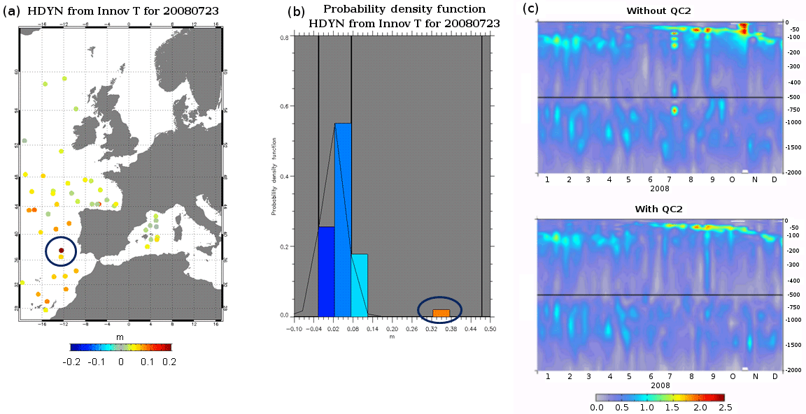
Figure 3Statistics in the Azores region: (a) absolute value of dynamical height innovations (in meters) from temperature innovations for the 7-day assimilation cycle from 16 to 23 July 2008; (b) PDF of theses dynamical height innovations (the value 0.3 m appears in the tail of the PDF); (c) RMS innovation with respect to the vertical temperature profiles over the year 2008 for two “twin” simulations (without and with QC2). Theses last scores are averaged over all 7 days of the data assimilation window, with a lead time equal to 3.5 days. Units are ∘C.
It should also be noted that the QC2 quality control rejects the entire vertical profile, while the QC1 quality control only rejects aberrant temperature and/or salinity values at some given depths on the vertical profile.
Figure 3a shows an example of a “wrong” temperature profile detected by the QC2 (and not by the QC1) at the end of July 2008. In this case, thresholdT is equal to 0.3 m (Fig. 3b). The first condition of Eq. (2) is satisfied and the profile is rejected. When this profile is assimilated (simulation without QC2), abnormal temperature RMS innovation values appear at the temporal position (July 2008) of this profile in the Azores region (Fig. 3c). Using QC2 quality control allows the problem to be solved for this particular profile but also for some other profiles (see Fig. 3c).
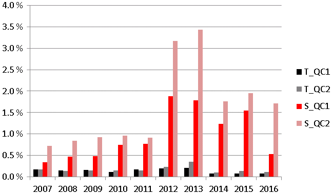
Figure 4Statistics of suspicious temperature (T) and salinity (S) detected by QC1 (T_QC1 and S_QC1) and by QC2 (T_QC2 and S_QC2) quality controls as a function of year in the PSY4V3 2007–2016 simulation time period.
Statistics of the QC1 and QC2 quality controls are summarized in Fig. 4, in which the percentage of suspicious temperature and salinity profiles is given as a function of the year over the 2007–2016 period. This percentage is relatively stable for both temperature and salinity profiles, with little year-to-year variability, except for the years 2012 and 2013 when more suspicious temperature and salinity profiles than usual were detected. Nevertheless, this percentage remains relatively low (less than 0.35 % for temperature and 3.5 % for salinity) given that the number of temperature profiles available each year ranges between 1.1 and 1.7 million number of salinity profiles between 150 000 and 600 000.
Most of the deficiencies in the systems can be related to these main recurring problems: initialization, atmospheric forcing biases, abyssal circulation and efficiency of the assimilation schemes. The first three problems are related to uncertainties in poorly observed areas or parameters (i.e., deep ocean, ice thickness) and to intrinsic errors of the atmospheric forcing. The last problem is related to linearity and stationarity hypotheses in the assimilation schemes. In this section, we detail some solutions adopted for the system PSY4V3, reducing uncertainties in the thermohaline component and allowing flow dependence in our assimilation scheme. These solutions correspond to a part of the updates mentioned in Sect. 2 that do not result from routine system improvements.
3.1 Initialization of oceanic simulation
One way to initialize physical ocean model simulations is by using climatological values of temperature and salinity from databases and assuming the velocity field is zero at the start. The model physics then spins up a velocity field in balance with the density field. Another common way to initialize a model is with fields from a previous run of that model or with the results from another model.
Given that data assimilation of the current observation network rapidly (in about 6 months) adjusts the model state in the first 1000 m, the first solution has been chosen to minimize potential drifts occurring after some years of simulation. Compared with the previous system PSY4V2 starting in October 2012 from the WOA09 three-dimensional climatology (see Fig. 1), the PSY4V3 system starts in October 2006 using improved initial climatological conditions. For that, we chose to use ENACT-ENSEMBLES EN4 1∘ global product (Good et al., 2013), which consists of monthly objective analyses. The great interest of these monthly fields is that a three-dimensional observation weight (between 0 and 1) describes the influence of the observations for each field. This information helps to retain only the observed points and not the perpetual climatology. This allows for the computation of validated trends for each month and of climatology for a particular date. For that, a point-wise linear regression, in particular Kendall's robust line-fit method (Hoaglin et al., 1983), is used, allowing us to obtain an initial condition called “robust EN4” for any time based only on real observations.
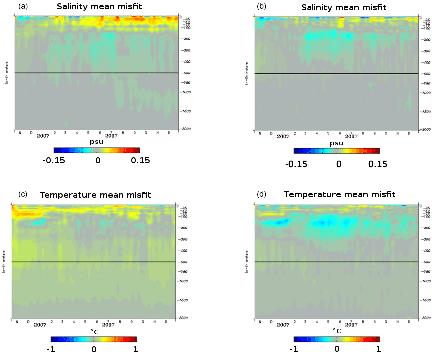
Figure 5Diagnostics (time series) with respect to the vertical temperature and salinity profiles over the October 2006–December 2007 period. Mean misfit between observations and model for salinity (a, b, units in psu) and for temperature (c, d, units in ∘C) starting from WOA09 climatology (a, c) and robust EN4 (b, d).
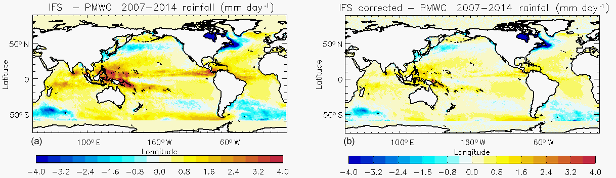
Figure 6Mean 2007–2014 IFS ECMWF atmospheric precipitation bias (units in mm day−1) with respect to PMWC product without (a) and with (b) correction.
Two free simulations (without any data assimilation) have been performed with the system PSY4V3 using either WOA09 or robust EN4 as an initial condition in October 2006. Figure 5 shows the box-averaged innovations of temperature and salinity as a function of time and depth over the October 2006–December 2007 period. Fig. 5a reveals that, using WOA09 as an initial condition, a fresh bias appears in the first 100 m of the innovation, particularly more pronounced at the surface. It is no longer the case when using robust EN4 to initialize the model (Fig. 5b). For temperature, Fig. 5c exhibits cold biases above 100 m and below 300 m that are considerably reduced by using robust EN4 as an initial condition (Fig. 5d). The warm and salty bias between 200 and 300 m is slightly reinforced. It mostly concerns the main thermocline whose motions are well correlated with the altimetry. This bias will be corrected by the assimilation of altimetry and Argo profiles. Deeper biases are reduced with this new initialization where Argo profiles are missing.
3.2 Correction of precipitation
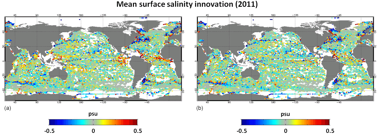
Figure 7Mean surface salinity innovation (difference between the assimilated observation and the model; units in psu) in the year 2011. (a) The innovation resulting from the use of the original IFS field, and (b) the innovation resulting from the use of the corrected IFS field.
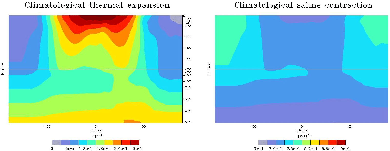
Figure 8Climatological thermal expansion (∘C−1) and saline contraction (psu−1) as a function of latitude and depth.
Many studies (e.g., Janowiak et al., 1998, 2010; Kidd et al., 2013) have compared reanalysis and atmospheric model precipitation fields with observation-based datasets and have shown that atmospheric model products always bring significant and systematic errors and are not able to close the global average freshwater budget. For instance, Janowiak et al. (2010) found that the IFS operational model and ERA-Interim reanalysis (Dee et al., 2011) from ECMWF perform well for temporal variability with respect to observational datasets, but they globally overestimate the daily precipitation. Although progress has been made in the ECMWF forecast model, substantial errors still occur in the tropics (Kidd et al., 2013). The correction of atmospheric forcing within ocean applications has already been successfully explored by adjusting atmospheric fluxes via observational datasets in global applications (Large and Yeager, 2009; Brodeau et al., 2010). Other studies only focused on precipitation correction (Troccoli and Kallberg, 2004; Storto et al., 2012).
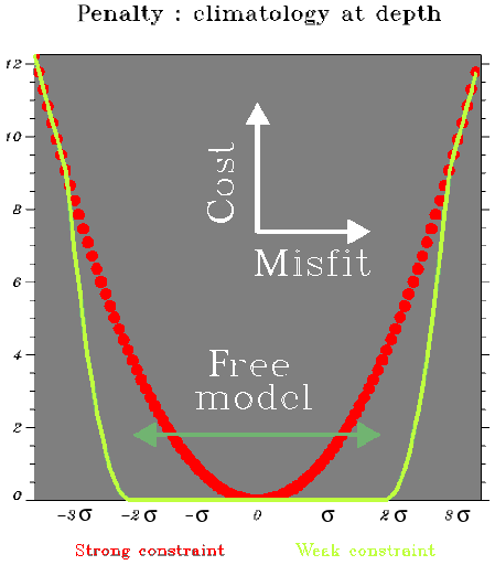
Figure 9Non-Gaussian error for climatology (corresponding to a weak constraint of the system in green). A cost equal to zero corresponds to an infinite observation error, namely a system operation in a free mode (without assimilation of climatology).

Figure 10Mean temperature (a, units in ∘C) and salinity (b, units in psu) innovations in 2013 at 2865 m for the system PSY4V3.
The proposed method in this paper consists of correcting the daily precipitation fluxes by means of a monthly climatological coefficient inferred from the comparison between the Remote Sensing Systems (RSS) Passive Microwave Water Cycle (PMWC) product (Hilburn, 2009) and the IFS ECMWF precipitation. We use the remote PMWC product because of its relatively high 1∕4∘ resolution able to more accurately represent narrow permanent features such as the Intertropical Convergence Zone. The use of a spatially varying monthly climatological coefficient is justified by the fact that the interannual variability is well captured by the ECMWF forecast model and allows us to apply the correction outside the special sensor microwave imager era. This latter assertion is a limitation of the method as it assumes the operational ECMWF forecast model has a constant bias. In order to avoid discontinuities when either PMWC or ECMWF products exhibit zero precipitation, e.g., in arid areas, we do not apply any correction in monthly mean values less than 1 mm for rainfall fluxes. Also, in order to keep the more accurate small-scale signal from the high-resolution forcing, the correction is only applied to the large-scale component obtained by a low-pass Shapiro filter. Hilburn et al. (2014) provided the accuracy of RSS over ocean rain retrievals validated against well-established long-term in situ datasets such as observations from Pacific Marine Environment Laboratory rain gauges on moored buoys in the tropics. They found that on monthly average, the standard deviation between satellite and buoy is 15.5 %. The differences are greatest in the Indian Ocean and western Pacific. We then arbitrarily capped the correction beyond 20 % in order to take into account these satellite-based retrieval errors. Lastly, we did not apply the correction poleward of 65∘ N and 60∘ S because of important biases in satellite-based precipitation estimates (Lagerloef et al., 2010) at high latitudes.
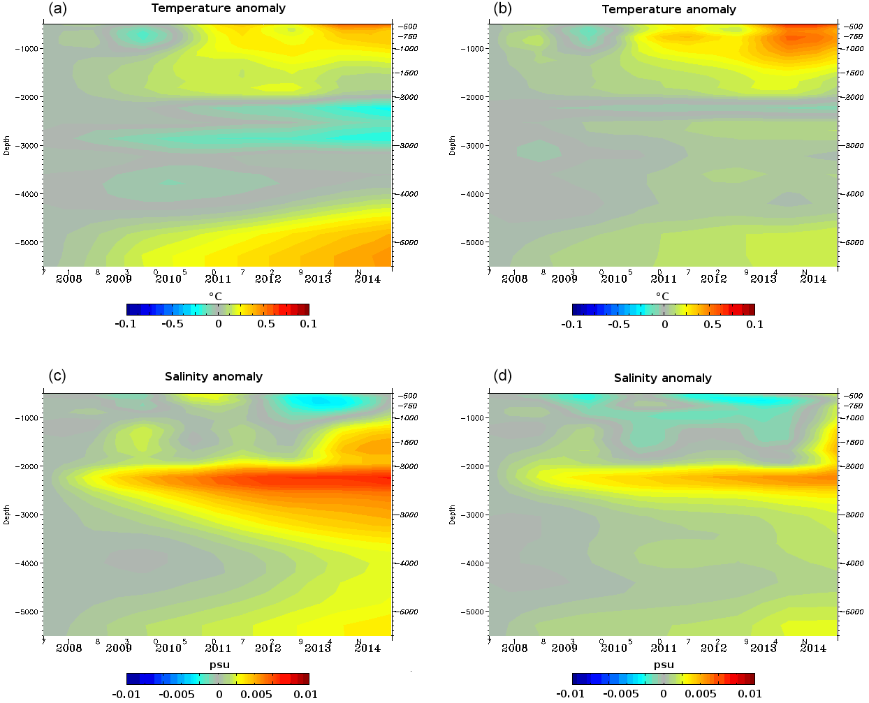
Figure 11Temperature (a, b, units in ∘C) and salinity (c, d, units in psu) annual anomalies over depth (500–5000 m) and time (2007–2014) for latitudes between 30 and 60∘ S. The simulation in (a) and (c) does not assimilate climatological vertical profiles, while the simulation in (b) and (d) assimilates them. Annual anomaly for a specific year is computed as the difference between the annual mean of this year and the annual mean of the year 2007.
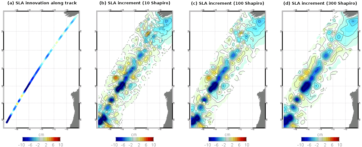
Figure 12SLA innovation along a single assimilated track altimeter (a). SLA increments with 10 (b), 100 (c) and 300 (d) Shapiro passes as anomaly filtering. These experiments have been performed with a regional system at 1∕36∘. Unit is centimeters.
Figure 6 represents the difference between the IFS precipitation coming from ECMWF and the PMWC product using satellite data before and after large-scale correction. As already pointed out by Stephens et al. (2010), original IFS forcings exhibit a systematic overestimation of precipitation within the intertropical convergence zones (up to 3 mm day−1) and underestimation at middle and high latitudes (up to −4 mm day−1). After correction, the mean bias compared with PMWC is reduced from 0.47 to 0.19 mm day−1.
To validate this correction, two global ocean hindcast simulations of several years, using only the 3D-VAR large-scale bias correction in temperature and salinity, have been performed, one with IFS correction and the other without. Figure 7 represents the mean surface salinity innovation (difference between the assimilated observation and the model) in the year 2011. At the global scale, the bias reduction is not very significant, but these maps demonstrate that the IFS correction is beneficial in many local areas. The strongest benefit concerns the tropics where the IFS correction allows us to reduce the magnitude of the near-surface salinity fresh mean bias down to 0.5 psu. The fresh bias reduction in the tropics reaches 0.15 psu on average.
3.3 Assimilation of climatological temperature and salinity climatology in the deep ocean
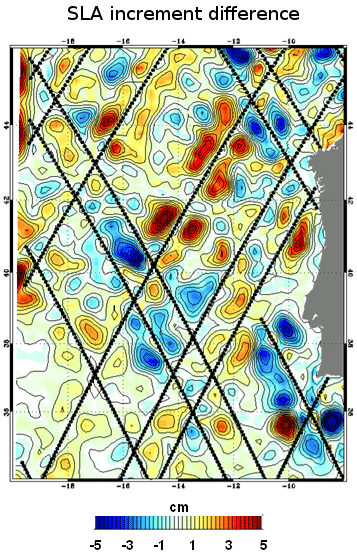
Figure 13SLA increment difference using 10 and 300 Shapiro passes as anomaly filtering in a regional system at 1∕36∘. The black lines represent the position of the assimilated altimeter tracks. Unit is centimeters.
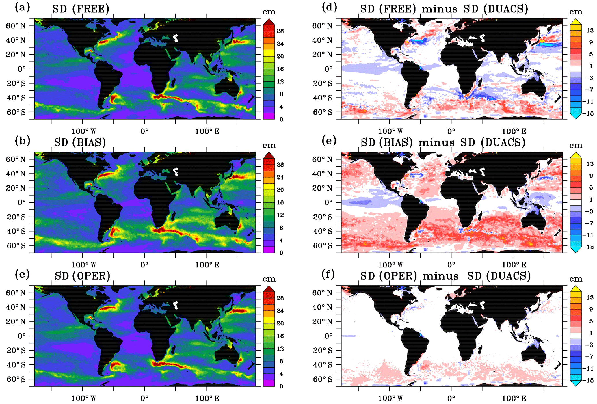
Figure 142007–2015 SSH standard deviation (diagnostics made with one point every three horizontally and 1 day every 5) of the 1∕12∘ PSY4 simulations (a, b, c) and difference of the SSH model standard deviation from the one of the DUACS gridded product (d, e, f). Units are centimeters.
The model may exhibit significant drift at depth that can be related to the misrepresentation of several processes, an exhaustive list of which would be hard to give here. Difficulties encountered by ocean models using z coordinates in overflow regions are likely to be largely responsible for this. In addition, Eulerian vertical coordinates (vs. Lagrangian, isopycnal coordinates) may add a spurious diapycnal component in the interior where mixing is essentially in the isopycnal direction. Lastly, the model lacks an accurate interior mixing scheme such as the one of De Lavergne et al. (2016) that does take into account internal tidal wave mixing (tides are not explicitly resolved in PSY4V3). Interior mixing is indeed crudely represented by spatially constant background diffusivity in the model.
For systems that assimilate observations in a multivariate way, the problem can be more critical because of the deficiencies of the background error covariances that may contain spurious correlations for extrapolated and/or poorly observed variables. Unfortunately, there are very few temperature and salinity profiles below 2000 m to constrain the model drift. Hence, the climatology is currently the only source of information at depth to prevent the model from drifting. Virtual vertical profiles of temperature and salinity below 2000 m are built from the monthly WOA13v2 climatology. These virtual observations are geographically positioned on the model horizontal grid with a coarse resolution (1∘ × 1∘) and on the model vertical levels from 2200 m to the bottom.
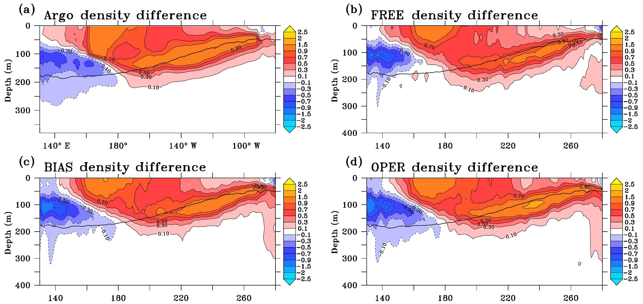
Figure 15Density difference (October–December 2008 minus October–December 2009) in the equatorial Pacific (2∘ S–2∘ N) above 400 m of depth (a–d) from the SCRIPPS Argo product (a) and the three 1∕12∘ PSY4 FREE, BIAS and OPER simulations (b–d). The black line indicates the 2007–2015 Argo mean position of the pycnocline depth (isopycn 1025 kg m−3).
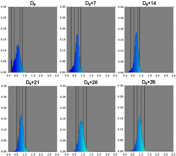
Figure 16Evolution of the PDF of the ratio for the Envisat satellite from D0 to D0 + 35 days. D0 corresponds to the first day when Envisat is assimilated by the system.
As in Greiner et al. (2006), we define empirically the standard deviations (departures from the climatology) σT for temperature and σS for salinity as a simple linear vertical profile:
where z is the depth (in meters).
We then define σTS as the density departure from the climatology:
where α represents the thermal expansion coefficient and β the saline contraction coefficient. Following Jackett and Mcdougall (1995), these coefficients are assumed to depend only on latitude and depth of the ocean as illustrated by Fig. 8.

Figure 17Envisat (a, b) and Jason2 (c, d) satellite observation errors used on the 7-day assimilation cycle ending 23 September 2009 without tuning (a, c) and with the tuning (b, d) method. Unit is centimeters.
If we denote dTS the density innovation, d the temperature or the salinity innovation, and σ the temperature or the salinity departure from the climatology, the value of the climatological error e is prescribed as
A non-Gaussian error is used to impose a weak constraint on the model at depth (Fig. 9). That way, we correct the model drift without constraining a slow moderate variability or trend. Basically, the hypothesis is that small to medium departures from the climatology (2σ or less) have an even probability. For instance, a 0.2 ∘C model warming at 2000 m due to a positive North Atlantic Oscillation pattern must not be corrected as zero. Indeed, a 0.2 ∘C cooling is as likely as the warming, since the climatology is the time average of those anomalies. So, only large departures from climatology (3σ or more) should be corrected. It corresponds to highly unlikely events that are typical of model drifts. An interesting point is that model drift is often corrected locally, downstream of the outflow, before it spreads out (see Fig. 10). Ideally, it gives a little regional correction instead of a large basin-scale bias.
To validate this kind of assimilation, two global ocean simulations of several years, using only the 3D-VAR large-scale bias correction in temperature and salinity, have been performed. Due to the high computational cost of the system PSY4V3, the assimilation of WOA13v2 below 2000 m has been tested with a global intermediate-resolution system at 1∕4∘, which in all other aspects is very close to the high-resolution system PSY4V3. All in situ observations have been used as well.
In practice, the assimilation of WOA13v2 climatological profiles below 2000 m in the system concerns mostly some regions where the steep bathymetry might be an issue for the model (Kerguelen Plateau, Zapiola Ridge, Atlantic Ridge). Figure 10 shows mean temperature (left) and salinity (right) innovations (WOA13v2 climatological profiles minus model) in 2013 at 2865 m. The assimilation of these climatological profiles occurs more or less at the same locations over the time period 2007–2016. Since the conditions of the system of Eq. (6) relate to the density innovation, we have a perfect symmetry of the temperature and salinity data that are assimilated. This has the effect of not disturbing the density gradients too much.
If we focus on latitudes between 30 and 60∘ S, Fig. 11 represents temperature (top panels) and salinity (lower panels) annual anomalies over depth (500–5000 m) and time (2007–2014). The simulation on the left does not assimilate climatological vertical profiles, while the simulation on the right assimilates some. These maps demonstrate that the assimilation of WOA13v2 below 2000 m is beneficial, reducing drifts below 2000 m. In the Antarctic Circumpolar Current (ACC), the assimilation of these profiles makes it possible to maintain, for instance, the Antarctic Bottom Water (see Gasparin et al., 2018). This also impacts the vertical repartition of the steric height without degrading the quality of the results compared to profiles from the Argo network.
3.4 Construction of the background error covariance
The seasonally varying background error covariance is based on the statistics of a collection of three-dimensional ocean state anomalies. This approach is based on the concept of statistical ensembles in which an ensemble of anomalies is representative of the error covariance. In this way, truncation no longer occurs and all that is needed is to generate the appropriate number of anomalies. The way in which these anomalies are computed from a long numerical experiment is described in Lellouche et al. (2013).
In this section, we detail two features of the system PSY4V3 compared to the previous system PSY4V2 regarding the construction of the background error covariance. First, we evaluate the impact of anomaly filtering on analysis increment. Second, we evaluate the potential added value to the quality of the analysis increments of the choice of the simulation from which to calculate the anomalies. In the previous system PSY4V2, a free simulation was used to calculate the anomalies. For the system PSY4V3, the anomalies are computed from a simulation in which only a 3D-VAR large-scale bias correction of T∕S has been performed.
3.4.1 Anomaly filtering
The signal at a few horizontal grid Δx intervals in the model outputs on the native full grid is not physical but only numerical (Grasso, 2000) and should not be taken into account when updating an analysis. This is why several passes of a Shapiro filter have to be applied at the anomaly computation stage in order to remove the very short scales that in practice correspond to numerical noise. This can also help to filter out the noise from the covariance matrix due to the sampling error (Raynaud et al., 2009). Another way to remove the very short scales would be to filter the analysis increments before injecting them into the model. This choice would have led to a less optimal analysis and to a loss of balance between the different components of the increment.
To illustrate the impact of the anomaly filtering, we set up some experiments with different levels of filtering. Each experiment consists of the assimilation of a single altimeter track over one assimilation cycle. These experiments have been performed with a Mercator Ocean regional system at 1∕36∘ using the SAM data assimilation scheme in order to reduce the high computing cost of the global system PSY4V3 and the time needed to build different sets of anomalies at the global scale. Figure 12 shows SLA increments obtained with these different levels of anomaly filtering. It should be noted that the anomaly filtering has a direct effect on the analysis increment, since the latter is a linear combination of the anomalies.
Figure 12a represents SLA innovation along the single assimilated track. Figure 12b, c and d represent the SLA increments obtained with 10, 100 and 300 Shapiro passes, respectively, as the anomaly filtering mentioned above (corresponding approximately to a 3, 10 and 15 horizontal grid Δx interval filter). We can see that the correction under the track remains more or less the same. The strongest differences occur outside the track where the innovation information is extrapolated.
Other experiments closer to real-time integration setup have been performed, assimilating all the altimeter tracks available in a 7-day assimilation window instead of one single track. Figure 13 shows the difference of SLA increments using 10 and 300 Shapiro passes as anomaly filtering (corresponding approximatively to 20 and 80 km). The conclusions are the same as those concerning the experiments with a single assimilated track. The corrections under the tracks remain almost the same for the two levels of filtering. Both analyses are close to the data under the tracks. The strongest differences occur outside the tracks where the innovation information is extrapolated to fill the gaps. Low-filtered increments (10 Shapiro passes) have small-scale structures that are statistical artifacts. Small structures can cascade in the model and stay trapped between the repetitive tracks without correction by the assimilation. This happens less when more filtering (300 Shapiro passes) is performed on the anomalies beyond the effective resolution of the model.
3.4.2 Choice of the simulation from which to calculate the anomalies
The system PSY4V3 was run over the October 2006–October 2016 period to catch up to real time (OPER simulation) starting from three-dimensional temperature and salinity initial conditions based on the EN4 climatology. This simulation benefited from the full data assimilation system, including the 3D-VAR bias correction and the SAM filter. Two other simulations over the same period have been performed. The first one is a FREE simulation (without any data assimilation) and the second one has exactly the same model tunings but only benefits from the temperature and salinity 3D-VAR large-scale bias correction (BIAS simulation).
Figures 14 and 15 show comparisons between this triplet of PSY4 simulations and two observational products. The first product is the CMEMS/DUACS (Data Unification and Altimeter Combination System) merged–gridded sea level anomaly heights in delayed time on a 1∕4∘ regular horizontal grid with a 1-day temporal resolution (Pujol et al., 2016). The second one is the Roemmich–Gilson Argo monthly climatology on a 1∘ regular horizontal grid (Roemmich and Gilson, 2009), which is commonly used in the oceanographic community. Figure 14a, b and c show the 2007–2015 SSH variability for the three simulations (subsampled in a similar way to DUACS). SSH variability difference is defined as the difference of SSH standard deviations from PSY4 simulations and the DUACS product (Fig. 14d, e, f). Compared to the variability of the DUACS product, the fronts in high-mesoscale-variability regions such as the Gulf Stream, the Kuroshio current, the Agulhas current or the Zapiola eddy are misplaced in the FREE simulation. In the BIAS simulation, these fronts are better positioned due to the large-scale correction of temperature and salinity. However, this simulation presents more energy compared to DUACS, apart from the main fronts. This corresponds to a leakage of vorticity from the fronts due to the mean advection. Note that the gridded DUACS product also underestimates the variability as wavelengths smaller than 200 km are barely resolved in the gridded fields. The effective resolution of DUACS product ranges from almost 500 km at the Equator to 150 km at high latitude. For the OPER simulation, the effective resolution is relatively similar or slightly larger in the intertropical band and almost 100 km at high latitude. The mesoscale features are well constrained in the OPER simulation with the information coming from satellite data.
Time-averaged density differences along the equatorial Pacific between two ENSO events (October–December 2008 minus October–December 2009), computed from the PSY4 simulations and from the Roemmich–Gilson Argo monthly climatology, are shown in Fig. 15. The SCRIPPS Argo product presents a higher density difference in the eastern part of the equatorial Pacific. It corresponds to the change from moderate La Niña conditions early in 2008 to moderate El Niño conditions in 2009. The FREE simulation is not dense enough in the east compared to observations, particularly at the pycnocline depth (1025 kg m−3 isopycn). The BIAS simulation intensifies the density difference. The OPER simulation gets even closer to the SCRIPPS Argo product. There is also an upward tilt of the density difference maximum in agreement with the observations.
In summary, the BIAS simulation better represents the density fronts on the horizontal (Gulf Stream) and on the vertical (Pacific pycnocline). The covariance matrix deduced from this simulation has information on the density gradients that is well placed. This is valuable off the Equator through geostrophy and at the Equator to control the zonal pressure gradient. The variance in sea level is stronger than the DUACS one (see Fig. 14e) but the most important point for the construction of the anomalies is to have well-placed density gradients. In the OPER simulation and as mentioned in Lellouche et al. (2013) in the description of the data assimilation system SAM, an adaptive scheme will correct the variance and will give an optimal background model error variance based on a statistical test formulated by Talagrand (1998).
3.5 Adaptive tuning of observation errors
In order to refine the prescription of observation errors (instrumental and representativeness errors), adaptive tuning of errors for the SLA and SST has been implemented in PSY4V3. We use the Talagrand method (Talagrand, 1998) to adjust the background error. Instrumental error does not change with time. On the contrary, the representativeness error is really flow dependent. Taking into account the representativeness error is particularly important for assimilated OSTIA SST because the sky is clear only 30 % of the time on average. The method has not been used for temperature and salinity vertical profiles because of the reduced number of in situ data compared with satellite data. Three-dimensional fixed observation errors are then used for the assimilation of in situ temperature and salinity vertical profiles.
The method consists of the computation of a ratio, which is a function of observation errors, innovations and residuals (Desroziers et al., 2005). It helps correct inconsistencies in the specified observation errors. This ratio can be expressed as
Ideally, ratio is equal to 1. When the ratio is less (larger) than 1, it means that the observation error is overestimated (underestimated). The objective of this diagnostic is to improve the error specification by tuning an adaptive weight coefficient acting on the error of each assimilated observation. As a first guess of the method, the initial prescribed observation error matches the one used in the previous system (Lellouche et al., 2013) in which the observation error variance was increased near the coast and on the shelves for the assimilation of SLA and increased only near the coast (within 50 km of the coast) for the assimilation of SST.
Figure 16 represents the temporal evolution of the ratio defined in Eq. (7) for the Envisat satellite. At the beginning of the simulation, the observation error is overestimated (ratio less than 1). The ratio tends to 1 after only a few weeks of simulation.

Figure 18Evolution in time of model SST anomaly (a) and SST observation error anomaly tuned by the Desroziers method (b) for a section at 3∘ N. The blue lines represent the beginning of La Niña episodes (mid-2007 and mid-2010). The black ellipses highlight periods when TIWs are more marked. Units are ∘C.
For SLA (Fig. 17), the a priori prescribed observation error is globally significantly reduced. The median value of the error changed from 5 to 2.5 cm in a few assimilation cycles and allows for better results. This method allows us to have more realistic and evolutive observation error maps that can provide valuable information for space agencies.
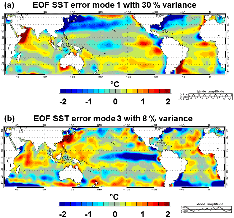
Figure 19First EOF (a) and third EOF (b) of sea surface temperature observation error (∘C) over the 2007–2015 time period. The time series at the bottom of each panel correspond to the mode amplitude.
The realism of tropical oceans is crucial for seasonal forecasting applications. Tropical instability waves (TIWs) can be diagnosed from SST (Chelton et al., 2000). These Kelvin–Helmholtz waves initiate at the interface between areas of warm and cold sea surface temperatures near the Equator and form a regular pattern of westward-propagating waves. Figure 18 gives an example of the adjustment of observation error to model physics and atmospheric variability. The SST anomalies in the equatorial Pacific clearly show the propagation westwards of TIWs in the second half of the year. This is more pronounced during episodes of La Niña (mid-2007 and mid-2010). The observation error anomalies estimated by the Desroziers method show that the error increases when these TIWs are more marked. This can be explained two ways. First, the representativeness error increases because the data are not corresponding exactly at the right time and the right position to the model counterpart. In the case of clouds, SST values can result from OSTIA time or space interpolation. This would be detrimental with the fast propagation of TIWs. Second, large errors can result from a model shift of the TIW structures. The error decreases in the reverse case.
We have also performed an empirical orthogonal function (EOF) analysis to assess the variability of the SST observation error (Fig. 19). Mode 1 is associated with the seasonal cycle and mode 2 (not shown) corresponds to the migration of the seasonal signal. Mode 3 is associated with the interannual signal with, for instance, the transition La Niña–El Niño, showing that the SST error is able to adapt to both seasonal and interannual fluctuations.
This section describes the PSY4V3 system's quality assessment with diagnostics over particular years, together with time series over multiyear periods. To evaluate the quality of the system, the departure from the assimilated observations (SST, SLA, T∕S vertical profiles and sea ice concentration) is measured. Moreover, the analyses are also compared with observations that have not been assimilated by the system such as tide gauges, velocity measurements from drifting buoys, NOAA SST and AMSR sea ice concentration. NOAA SST and AMSR sea ice analyses are not fully independent, since the upstream observations are the same as for assimilated CMEMS OSTIA SST and OSI sea ice concentrations, but comparisons to a variety of estimates using different algorithms and protocols provides a useful consistency analysis.
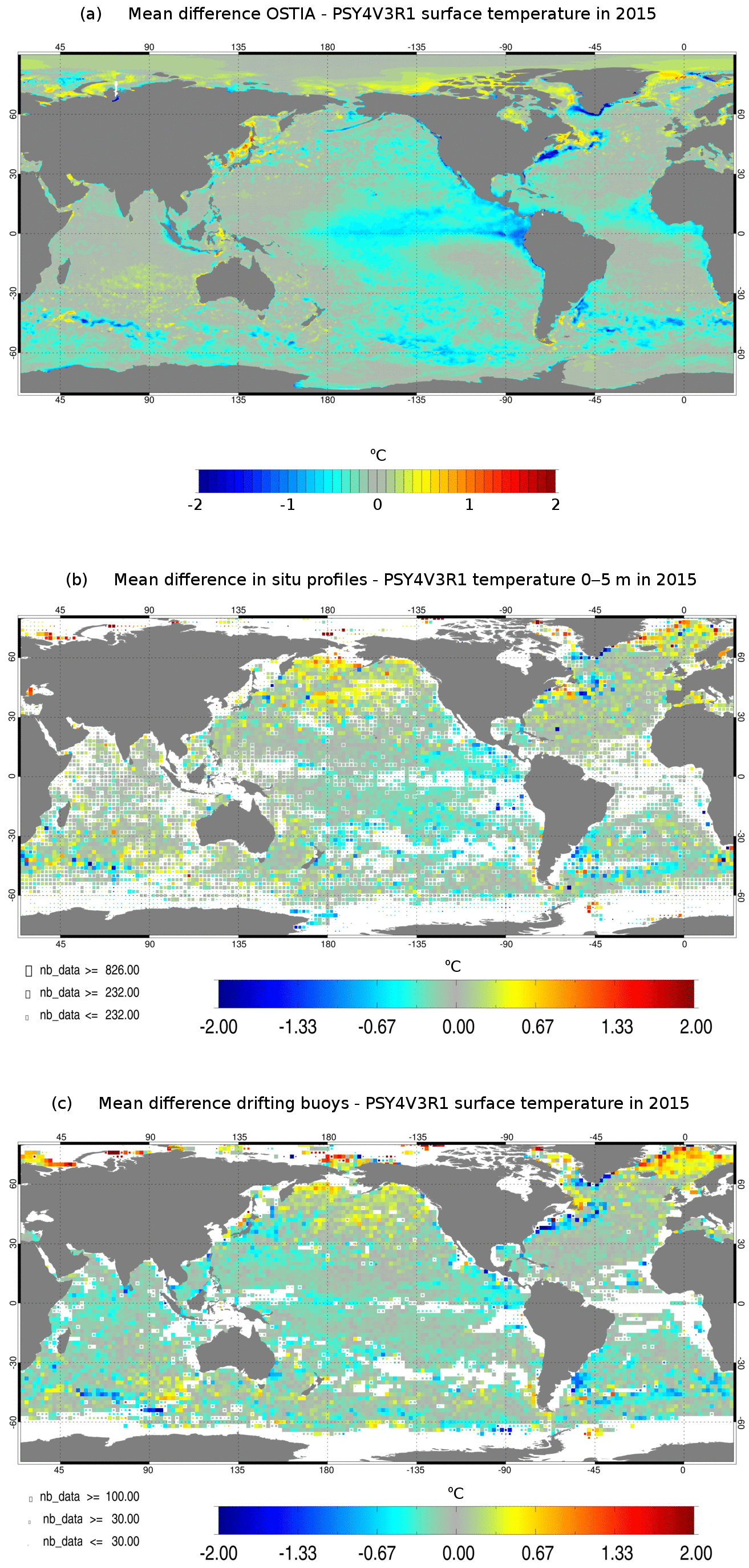
Figure 20Mean SST residuals (units in ∘C) over the year 2015: OSTIA SST minus PSY4V3 (a), in situ SST minus PSY4V3 (b) and drifting buoys SST minus PSY4V3 (c).
4.1 SST
4.1.1 Assimilated SST
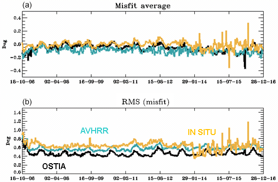
Figure 21Time series of SST (units in ∘C) global misfit average (a) and RMS (b) for OSTIA observations (black line, assimilated), NOAA AVHRR observations (blue line, not assimilated) and in situ observations (orange line, assimilated) from October 2006 to December 2016.
The OSTIA product is assimilated in the system PSY4V3. Compared to the previous system PSY4V2, some large-scale cold biases with respect to OSTIA are reduced in the Indian, eastern South Pacific and western North Pacific oceans (not shown). On the other hand, warm biases are not reduced, especially in regions of strong interannual warm events such as the eastern tropical Pacific where strong El Niño took place in 2015/2016, but also in the ACC, the Gulf Stream and the Greenland Current (Fig. 20a). Some inconsistencies can be found between OSTIA SST and in situ near-surface temperature, particularly in the North Pacific where the system PSY4V3 presents a cold bias compared to in situ near-surface temperature but a warm bias compared to OSTIA SST (Fig. 20b). Figure 20c shows the difference between drifting buoy SST and the system PSY4V3 over the year 2015. The drifting buoy SST data are present in the CMEMS in situ database used by Mercator but they have not been assimilated in the system because the depth of these data is a nominal value and we chose to assimilate only data with a measured depth value. Although we plan to assimilate these data in the future system, we use currently these data as independent information. This allows us to see that SSTs from in situ vertical profiles and SSTs from drifting buoys are coherent with each other. We thus again find the cold bias highlighted by the comparison with SST from in situ vertical profiles in the North Pacific. It is a lack of stratification in the model that causes midlatitude cold surface biases during (boreal) summer and a warm bias between 50 and 100 m.
We also checked the time series of the mean and the RMS of the misfit (innovation) between the observed SSTs and the model. For OSTIA SST, which is the gridded SST assimilated into PSY4V3, we obtain a mean warm bias of −0.1 ∘C and an RMS error of 0.45 ∘C (Fig. 21). Time series of the differences between the model and NOAA AVHRR SST, which was assimilated into the previous PSY4V2 system, are also shown in Fig. 21. This allows us to compare both gridded SST products. For in situ SST, the bias is smaller, suggesting that OSTIA and AVHRR are colder than in situ near-surface observations on global average. We can notice a drop in the RMS of in situ surface data in January 2014, which is due to the use of near-real-time observations for which most of the surface observations do not have a sufficient quality flag.
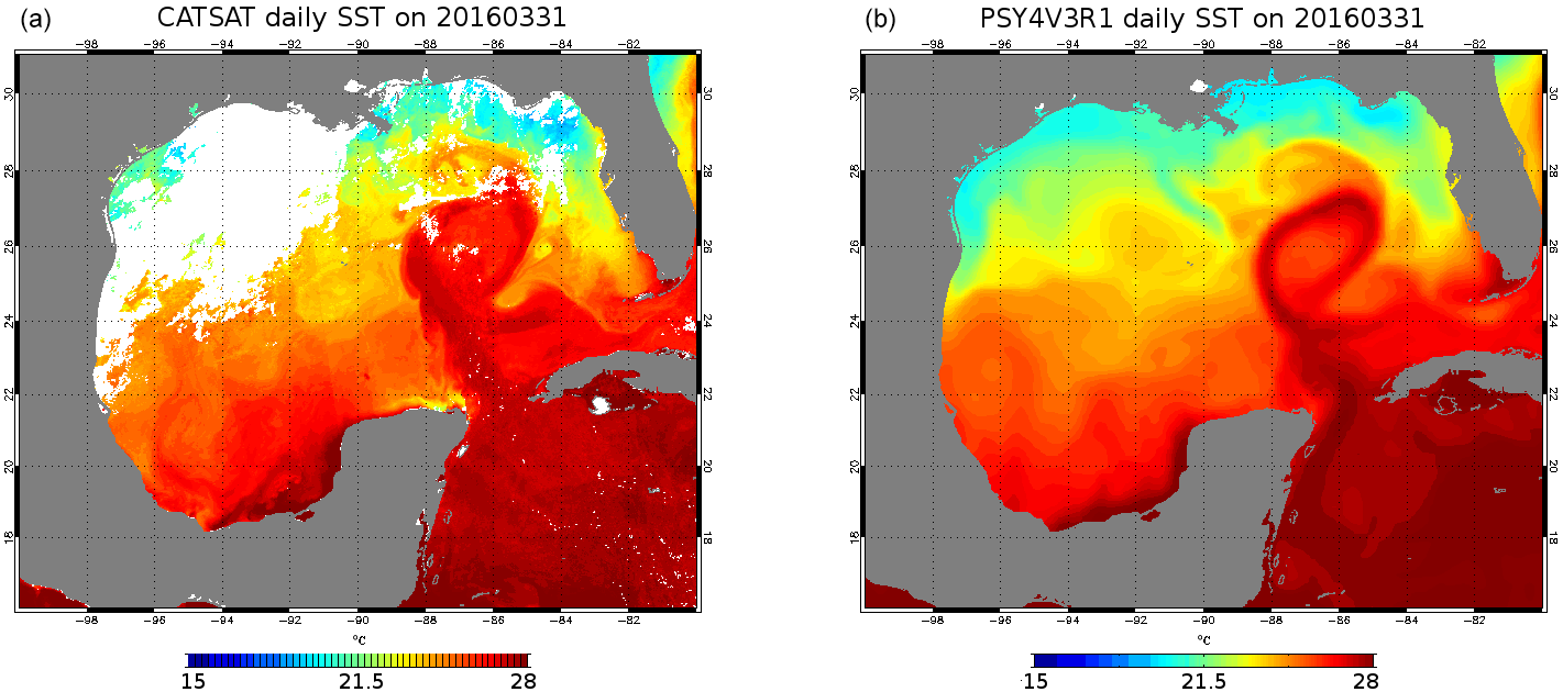
Figure 22High-resolution CATSAT SST from CLS (a) and PSY4V3 SST (b) on 31 March 2016. Unit is ∘C.
4.1.2 Comparison with a high-resolution SST external product
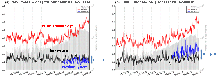
Figure 23Time series of the 0–5000 m RMS difference between the model analysis and the in situ observations for the previous system PSY4V2 (in blue), the new system PSY4V3 (in black) and the WOA13v2 climatology (in red). (a) Temperature (unit in ∘C), (b) salinity (unit in psu). Time series of the number of available observations appear in grey.
The CLS (Collecte Localisation Satellites) has operated a near-real-time oceanography data service named CATSAT since 2002 for scientific, institutional or private users (support to fishery management or to the offshore oil and gas industry). These data include satellite observations such as chlorophyll a, SST and altimetry. Maps of SST are computed from Aqua/MODIS, S-NPP/VIIRS and Metop/AVHRR infrared sensors at 2 km resolution using nighttime data only to avoid diurnal warming effects. We can then evaluate the system ability to produce mesoscale features by comparing with the CATSAT daily SST product. In Fig. 22, the CATSAT daily snapshot can be considered as an independent dataset since the OSTIA SST assimilated into the system has mostly seen microwave measurements during 2 weeks, as it was very cloudy in the Gulf of Mexico. 31 March 2016 is the first day clearly showing, from infrared measurements, the loop current and other structures in the western part of the Gulf of Mexico. The loop current is almost forming a closed meander. This is reproduced by the system PSY4V3, as are secondary structures like the filament in the north (Fig. 22). Visible limitations of this 1∕12∘ system concern the fine sub-mesoscale features that cannot be resolved and the lack of tidal mixing along Yucatan coasts (Kjerfve, 1981).
4.2 Temperature and salinity vertical profiles
For the T∕S vertical profiles, we checked time series of the RMS of the difference between the model analysis and the observations for temperature and salinity (Fig. 23a and b, respectively) in the whole water column. We compare observation and climatology (red line), the previous system PSY4V2 (blue line), and the new system PSY4V3 (black line).

Figure 24Mean residual errors (a, b) and RMS residual errors (c, d) of SLA in 2015 for the previous system PSY4V2 (a, c) and the new system PSY4V3 (b, d). Unit is centimeters.
On global average and compared to the previous system PSY4V2, the system PSY4V3 slightly degrades the temperature statistics (−0.03 ∘C) but greatly improves the salinity statistics by decreasing the 0–5000 m RMS salinity by 0.1 psu. This enables us to get a more accurate description of the water masses. This better balance arises from new in situ errors that give more weight to the salinity data (not shown). We can also notice that the systems are always better than the climatology. The comparison to climatology is a minimum performance indicator that the system must achieve. The differences with the climatology are worse from the beginning of the year 2013. It can be explained by the fact that six different decades of WOA13v2 monthly climatology can be found on the NODC website from 1955 to 2012. We chose the available 2005–2012 “truncated decade” (near our time period simulation) even if it is biased to cold given the strong La Niña event in 2010–2011. Previous decades (before 2005) are even colder and can no longer be used for recent dates. Moreover, the 2005–2012 truncated decade does not contain the period of transition towards El Niño events, in particular the strong one occurring in 2015. So, the in situ temperature and salinity vertical profiles we assimilated into the system and that see this transition are coherent with this WOA13v2 product until the end of the year 2012; this is no longer the case afterward.
Moreover, the system PSY4V3 experiences a slight warm bias (negative observation minus forecast difference) in the subsurface (25–500 m) on global average (not shown). For the year 2015, part of this signal comes from the strong interannual ENSO signals in the tropical Pacific where the near-surface bias is also warm, as well as in the ACC and the Gulf Stream. Seasonal cold surface biases appear in the midlatitudes, linked with a lack of stratification during summer. Summer warming is injected too deep, which results in subsurface spurious warming and a mixed layer that is too shallow. However, these biases remain small on global average.
4.3 Sea level
4.3.1 Assimilated SLA
The system PSY4V3 is closer to altimetric observations than the previous one with a global forecast RMS difference of around 6 cm instead of 7 cm for the system PSY4V2 (not shown). This RMS difference is consistent with the prescribed a priori observation errors (about 2 cm for altimeter instrumental error and 4 cm for MDT error on average). The statistics come from the data assimilation innovations computed from the forecast used as the background model trajectory and give an estimate of the skill of the optimal model forecast. These scores are averaged over all 7 days of the data assimilation window, which means the results are indicative of the average performance over the 7 days, with a lead time equal to 3.5 days.
More precisely, in the year 2015, the SLA mean and RMS errors are considerably reduced in the new system PSY4V3 compared to the previous one (Fig. 24). The mean bias is reduced by 0.3 cm (from −0.8 to 0.5 cm) and the RMS is reduced by 2.4 cm (from 7.9 to 5.5 cm). This is mainly due to the use of the Desroziers method to adapt the observation errors online, which yields more information from the observations being used (see Sect. 3.5). These improvements occur in nearly all regions of the ocean but are more pronounced in some regions (e.g., North Atlantic, Hudson Bay, Labrador Sea). In some others regions (e.g., Indonesian or west tropical Pacific), some errors in sea level remain and are linked to the uncertainty in the MDT or missing parameterizations in the model (interaction between wave and current, tides).
Figure 25Sea surface height RMS difference between tide gauge observations and the system PSY4V3 for the year 2015. Unit is centimeters.
4.3.2 Comparison to tide gauge data
The system PSY4V3 produces hourly outputs at the surface that can be compared with tide gauge measurements. For that, we used the BADOMAR product (Lefevre et al., 2005), which is a specific processed tide gauge database developed and maintained at CLS that consists of filtered tide gauge data from the GLOSS/CLIVAR (Global sea Level Observing System/Climate Variability and Predictability) “fast” sea level data tide gauge network (GLOSS Implementation Plan, 2012). These tide gauge data are corrected for inverse barometer effect and tides. High-frequency model SSH compares well with tide gauges in many places, with a slight improvement in PSY4V3 with respect to PSY4V2 (not shown). The best agreement between the system PSY4V3 and tide gauges is found in the tropical band, as can be seen in Fig. 25, while shelf regions and closed seas are less accurate. This confirms the latitude dependence of the correlation between tide gauges and satellite altimetry or modeled SSH discussed in Vinogradov and Ponte (2011) or Williams and Hugues (2013).
The improvements related to water masses and SLA lead to a correct global mean sea level (GMSL) trend. We checked the system GMSL by comparing the results with recent estimated trends from the paper of Chambers et al. (2017). We found for the model a trend of 3.2 mm yr−1 over the PSY4V3 simulation time period coherent with the DUACS value (3.17±0.67 mm yr−1). Moreover, the temporal evolution of the global mean model SSH is coherent and phased with the observations.
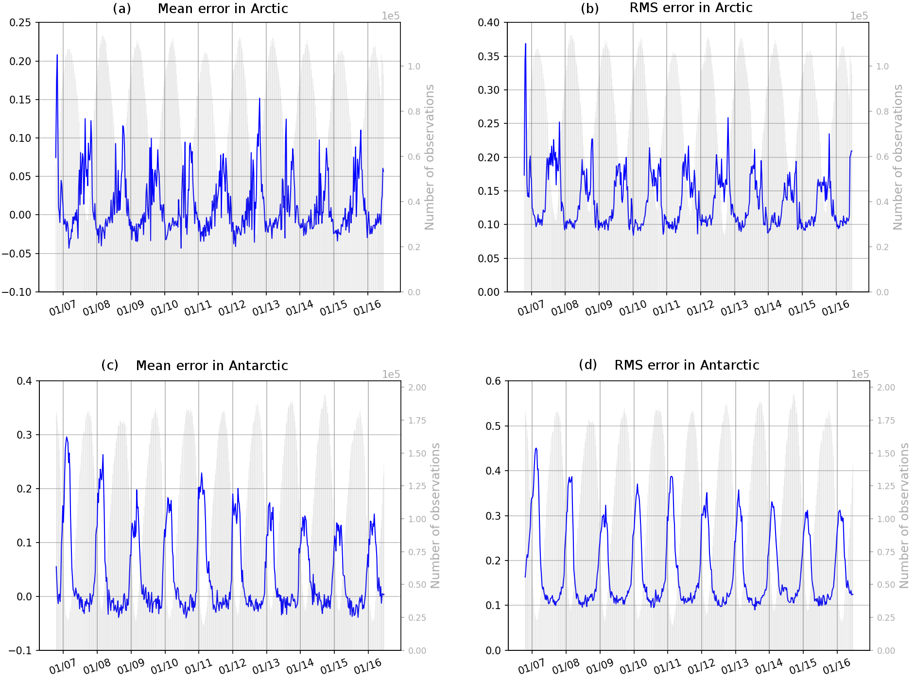
Figure 26Time series of (observation–forecast) mean (a, c) and RMS (b, d) differences of sea ice concentration (0 means no ice, 1 means 100 % ice cover) in the Arctic Ocean (a, b) and Antarctic Ocean (c, d). The assimilated observations are the sea ice concentrations from OSI TAC. Time series of the number of available observations appear in grey.
4.4 Sea ice concentration
4.4.1 Assimilated sea ice concentration
The system PSY4V3 assimilates OSI SAF sea ice concentration in both hemispheres with a monovariate–monodata scheme. As expected, PSY4V3 is closer to the observations than the previous system PSY4V2 (not shown), in which no sea ice observations had been assimilated. As illustrated by Fig. 26, the system PSY4V3 has a slight overestimation of ice during the melting season in summer (up to 3 % on average in both hemispheres). Conversely, the mean error is stronger on average during winter (10 % to 20 % underestimation, depending on the year). RMS errors are also larger during summer (up to 20 % in the Arctic and 30 % in the Antarctic with respect to OSI SAF observations), and they drop to less than 10 % in winter. These RMS errors quantify the capacity of the system to capture weekly time changes in the ice cover.
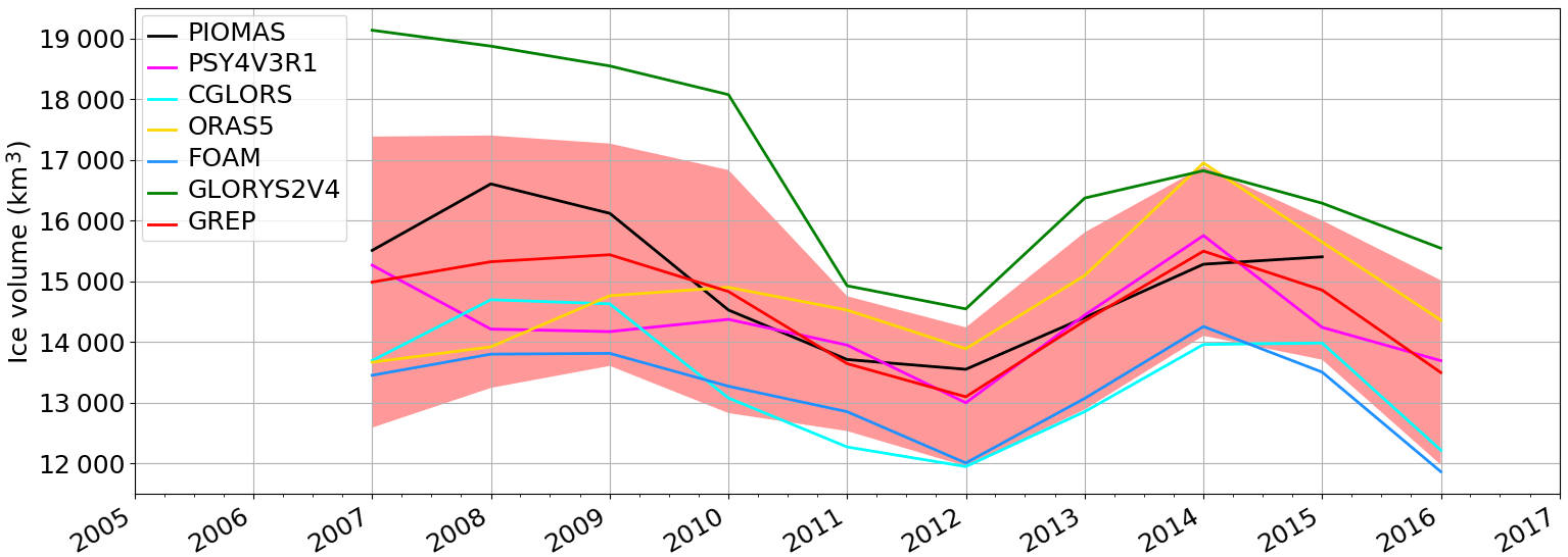
Figure 27Time series over the 2007–2016 period of sea ice volume in the Arctic for several systems: GREP composed of the four members GLORYS2V4 from Mercator Ocean (France), ORAS5 from ECMWF, FOAM/GloSea from the Met Office (UK) and C-GLORS from CMCC (Italy); PSY4V3 from Mercator Ocean (France); PIOMAS product. The spread of the GREP product is represented in light red. Unit is km3.
We have also checked the evolution of the sea ice volume diagnosed by the system PSY4V3. The data assimilation scheme SAM produces an increment of sea ice concentration, which is the unique sea ice correction applied in the model using the incremental analysis update (IAU) method described in Lellouche et al. (2013). The sea ice volume then adjusts to this correction considering a constant sea ice thickness. No sea ice thickness observations are assimilated in the system. The risk is therefore to obtain unrealistic drifts or trends of the unconstrained sea ice volume. Presently, sea ice volume retrievals from satellites are associated with large uncertainties (Zygmuntowska et al., 2014). Consequently, modeled sea ice volume is difficult to validate and one of the solutions is to compare modeled sea ice volume from several systems.
Figure 27 shows the 2007–2016 evolution of sea ice volume for the system PSY4V3, the PIOMAS modeled product (Schweiger et al., 2011) and the CMEMS GREP (Global Reanalysis Ensemble Product; http://marine.copernicus.eu/documents/QUID/CMEMS-GLO-QUID-001-026.pdf, last access: 20 September 2018) composed of four global 1∕4∘ reanalyses and the ensemble mean with the associated spread from the four members. All the modeled sea ice volumes present the same 2007–2016 interannual variability. PSY4V3 and PIOMAS are included in the spread whose range decreases over time from 4000 km3 in 2007 to 3000 km3 in 2012 and remains almost constant afterward. The GLORYS2V4 reanalysis is known to have a large sea ice volume compared to other reanalyses (Chevallier et al., 2017). Although we use the same method for the assimilation of sea ice concentration in GLORYS2V4 and PSY4V3, the sea ice volume diagnosed by PSY4V3 has values ranging between 13 000 and 15 800 km3, in better accordance with GREP and PIOMAS products.
4.4.2 Contingency table analysis
The contingency table analysis approach described in Smith et al. (2016) has been applied to evaluate sea ice extent as compared to observation. Satellite ice concentration coming from AMSR2 (L1B brightness with a NASA team 2 algorithm to compute sea ice concentration) has been used as an independent observation to provide a general assessment in the detection of false alarms for ice coverage. Although this type of evaluation is usually done on forecasts, we used hindcasts. For the computation of the statistics we have used a stereo-polar grid at a 20 km resolution. In each cell of that grid we have then computed binary values corresponding to ice–open water conditions for the model and the sea ice observations by using a 40 % concentration threshold. We have also restricted our study to the proportion correct total (PCT), following the conclusion of Smith et al. (2016) that it was more insightful to refer to the PCT rather than other proportions. The PCT quantity is defined as PCT = (hit ice + hit water) n−1 (see Table 3), where n is the total number of observations with a sea ice concentration greater than 15 %. A value of 1 corresponds to a perfect score.
Table 3Contingency table entries for sea ice verification of the PSY4V3 system compared to AMSR sea ice concentration observations.
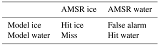
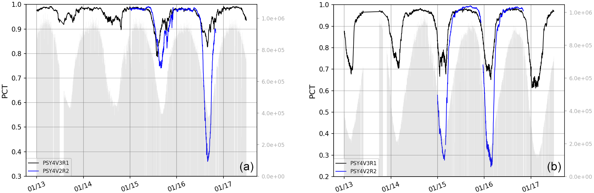
Figure 28Time series of the PCT quantity for PSY4V2 (in blue) and PSY4V3 (in black). (a) Corresponds to the Arctic and (b) to Antarctic. Time series of the number of available observations appear in grey.
Figure 28 shows times series of PCT for the PSY4V2 and PSY4V3 systems. The lower PCT values are mostly due to an excessive melt in spring and summer for both the Arctic and Antarctic. However, the assimilation of sea ice concentration significantly improves the total hit rate during these periods.
4.5 Currents
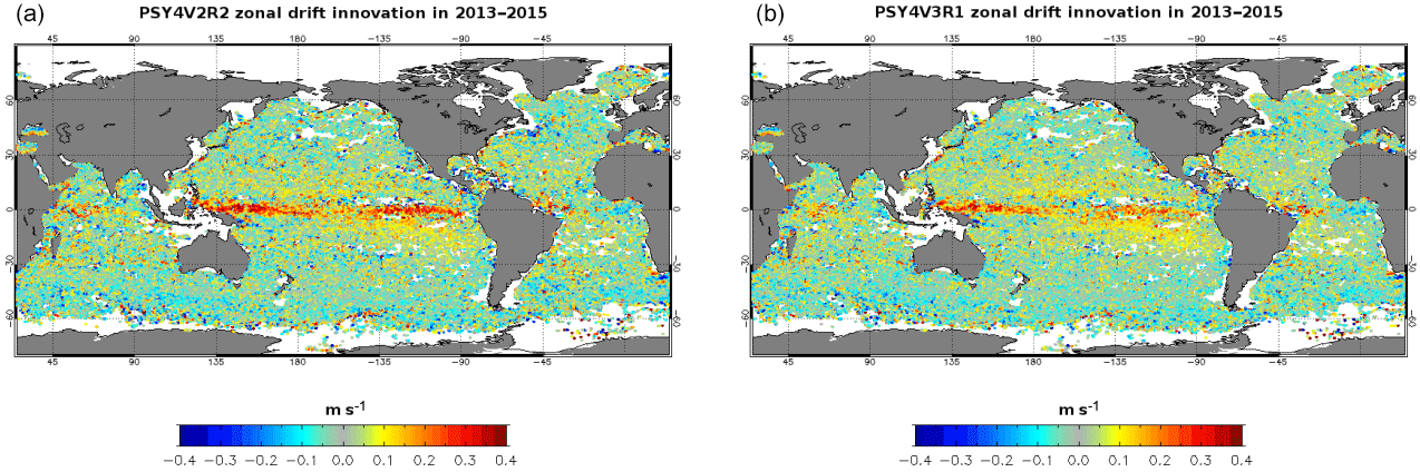
Figure 29Mean zonal drift innovation (m s−1) with PSY4V2 (a) and PSY4V3 (b) over the time period 2013–2015. Observations come from Argo surface floats and a surface-drifter-corrected dataset (Rio, 2012). Units are m s−1.
The aim of this section is to use velocity observations that were not assimilated into the system to assess the level of performance of PSY4V3 compared to the previous PSY4V2 system. The mean currents are checked by comparing the model to velocity observations coming from Argo floats when they drift at the surface and in situ Atlantic Oceanographic and Meteorological Laboratory (AOML) surface drifters. A paper by Grodsky et al. (2011) revealed that an anomaly in the drogue loss detection system of the Surface Velocity Program buoy had led to the presence of undetected undrogued data in the “drogued-only” dataset distributed by the Surface Drifter Data Assembly Center. Rio (2012) applied a simple procedure using altimeter and wind data to produce an updated dataset, including a drogue presence flag as well as a wind slippage correction. Therefore, we used this new drogued-only surface drifter dataset coming from CMEMS in situ TAC (Rio and Etienne, 2017) to check mean model currents.
Figure 29 represents zonal drift innovation for the PSY4V2 and PSY4V3 systems. Although some biases persist, mostly in the western tropical basins, significant improvements are obtained almost everywhere with the new system PSY4V3, particularly in the equatorial Pacific. The mean bias is reduced (from 0.1 to 0.08 m s−1), the South Equatorial Current is slower and there is also less noise in PSY4V3. Improvements are also obtained, to a lesser extent, for meridional drift (not shown). The velocities have been slightly improved in terms of velocity values but also in terms of current direction (angle between observed and modeled velocities). The mean angle difference is reduced from 9.1 to 7.2∘. These improvements can be attributed to the new MDT used and the more adapted filtering of anomalies. However, large biases persist in the western tropical Pacific (very strong in 2015 because of the strong El Niño event) with a spurious extension of the northern branch of the South Equatorial Current. This is probably linked to the uncertainty still present in the MDT and unresolved or missed parameterized physical processes.
More locally, a comparison of the 2007–2015 averaged drifts from the system PSY4V3 and the observations over the Indonesian region has been performed (not shown). Currents in this region are very difficult to resolve because of the many narrow straits and the strong tidal mixing. The retroflection of the westward South and North Equatorial Current (along Papua and near 12∘ N) into the eastward North Equatorial Countercurrent (near 4∘ N) are well-reproduced structures in the Pacific. The South Equatorial Current system is slightly too strong at the edge of the warm pool but this is the only significant weakness. The complex flow in the Sulawesi Sea, the Makassar Strait and the South China Sea is also reproduced well by the system. The correlation is 0.70 (0.64) for the zonal (meridional) velocity.
The Mercator Ocean system PSY4V3, in operational mode since 19 October 2016, benefits from many important updates. PSY4V3 has a quite good statistical behavior with an accurate representation of water masses, surface fields and mesoscale activity. Most of the components of the system PSY4V3 have been improved compared to the previous version: global mass balance, three-dimensional water masses, sea level, sea ice and currents. Major variables like sea level and surface temperature are hard to distinguish from the data.
In this paper, the updates showing the highest impact on the product quality and that do not result from routine system improvements have been illustrated and evaluated separately. Particular focus was therefore on the initialization, correction of precipitation, assimilation of climatological temperature and salinity in the deep ocean, construction of background error covariance and the adaptive tuning of observation error.
The initial climatological condition has been improved in order to be more consistent with the vertical profiles of temperature and salinity that have been assimilated thereafter. Rather than directly taking the climatological temperature and salinity of the month corresponding to the start of the simulation, we performed a point-wise linear regression, allowing us to obtain an initial condition at the appropriate time and based only on real observations; 1-year free simulations have been performed and show that biases are globally reduced.
Uncertainties inherent to atmospheric analyses and forecasts can induce large errors in ocean surface fluxes. For instance, a slight shift in the position of a storm can induce local errors in salinity, temperature and currents. In the tropical band, precipitation is systematically overestimated. Moreover, large-scale salinity biases can appear because the global average freshwater budget is not closed. For this reason, IFS ECMWF atmospheric analyzed and forecasted precipitation has been corrected at large scale using the satellite-based PMWC product. This correction is beneficial in many areas, reducing the magnitude of the near-surface salinity fresh mean bias in the tropics down to 0.5 psu. This surface fresh bias reduction in the tropics reaches 0.15 psu on average.
Due to misresolved processes, the model may also drift at depth. To keep some water mass properties, the DRAKKAR group restored modeled temperature and salinity toward the annual climatology of Gouretski and Koltermann (2004) in specific areas. This choice was driven by the Antarctic Bottom Water restoring zone where this climatology is recognized as more suitable. For Mercator systems that assimilate observations in a multivariate way, the problem can be more critical because of the deficiencies of the background errors for extrapolated and/or poorly observed variables. To overcome these deficiencies, vertical climatological T∕S profiles have been assimilated below 2000 m using a non-Gaussian error at depth, allowing the system to capture a potential climate drift in the deep ocean. In practice, the assimilation of climatological profiles below 2000 m in the system PSY4V3 concerns mostly some regions where the steep bathymetry might be an issue for the model (Kerguelen Plateau, Zapiola Ridge, and Atlantic ridge). This kind of assimilation reduces drifts below 2000 m and impacts the vertical repartition of the steric height without degrading the quality of the results compared to the profiles from the Argo network.
We have also proposed solutions to reduce some problems related to linearity and stationarity hypotheses in the assimilation schemes. The first one concerns the construction of background error covariance. Rather than calculating the anomalies from a free simulation, we chose to calculate them from a simulation benefiting only from the 3D-VAR large-scale bias correction in temperature and salinity and better representing the density fronts on the horizontal and on the vertical. Moreover, anomalies have been filtered in order to remove the scales beyond the effective resolution of the model. The second one concerns the tuning of the observation errors. Adaptive tuning of SLA and SST errors has been successfully implemented. It allows us to have more realistic and evolutive SLA and SST error maps.
All these scientific and technical choices have been validated and integrated into the system PSY4V3, which has been evaluated for the period 2007–2016 by means of a thorough procedure involving statistics of model departures from observations. The system PSY4V3 is close to SLA along-track observations with a forecast (range 1 to 7 days) RMS difference below 6 cm. Moreover, the correlation of the system PSY4V3 with tide gauges is significant at all frequencies; however, many high-frequency fluctuations of the SSH might not be captured by the system because tides or pressure effects are not yet included. The description of the ocean water masses is very accurate on average and departures from in situ observations rarely exceed 0.5 ∘C and 0.1 psu. In the thermocline, RMS errors reach 1 ∘C and 0.2 psu. In high-variability regions like the Gulf Stream, the Agulhas current or the eastern tropical Pacific, RMS errors reach more than 2 ∘C and 0.5 psu locally. A warm bias persists in the subsurface, with peaks in high-variability regions such as the eastern tropical Pacific, Gulf Stream or Zapiola. Most departures from observed SST products do not exceed the intrinsic error of these products (around 0.6 ∘C).
A global comparison with independent velocity measurements (surface drifters) shows that the location of the main currents is very well represented, as is their variability. However, surface currents of the midlatitudes are underestimated on average. The underestimation ranges from 20 % in strong currents to 60 % in weak currents. Some equatorial currents are overestimated, and the western tropical Pacific still suffers from biases in surface currents related to MDT biases. In contrast, the orientation of the current vectors is better represented.
Lastly, the system reproduces the sea ice seasonal cycle in a realistic manner. However, compared to assimilated data, sea ice concentration is slightly overestimated in winter seasons and underestimated during summer seasons. A contingency table analysis approach has also been used to evaluate sea ice extent compared to observations. This approach shows clear improvements due to the assimilation of sea ice concentration in the system PSY4V3.
Remarkable improvements have been achieved with the system PSY4V3 compared to the previous version. However, some biases have been highlighted in ocean surface features as well as three-dimensional ocean structure at basin, sub-basin and local scales. The simulation biases may be due to the initial state (especially in the deep layer for which historical observation data are rare), the atmospheric forcing uncertainties, the river runoff approximations, the efficiency of the assimilation scheme, and the model errors induced by unresolved or parameterized physical processes. Numerous projects have already been set up at Mercator Ocean to propose innovative solutions. The integration of the ingredients from these projects into the future CMEMS global high-resolution system is planned for 2019. The improvement of numerical simulations could thus be carried out based on sensitivity experiments on some model parameters (e.g., coastal runoffs, atmospheric forcing, high-frequency phenomena including tides, multi-category sea ice model, interaction and retroaction between ocean currents and waves, vertical mixing and advection scheme). Better algorithms and more sophisticated parameterizations already available in version 3.6 of the NEMO code should help in the future to resolve issues related to important ocean processes and to reduce model biases. It is also planned to assimilate new types of observations into the system (drifting buoys SST, higher-resolution SST (L3 products), satellite sea surface salinity, velocity observations from AOML surface drifters, deep-ocean observations from Argo surface floats) to better constrain the modeled variables and to overcome the deficiencies of the background errors, in particular for extrapolated and/or poorly observed variables. Another important issue is to use a shorter assimilation time window and a 4-D analysis in the assimilation scheme to better correct the fast-evolving processes. The next version of the global high-resolution system will also include seasonal errors for in situ vertical profiles already used in the CMEMS eddy-resolving 1992–2016 reanalysis GLORYS at 1∕12∘ horizontal resolution, which is based on the system PSY4V3 and appeared in the CMEMS catalogue in April 2018.
No datasets were used in this article.
JML designed and wrote the paper. JML and OLG performed the numerical simulations. JML and EG carried out most of the analyses, with contributions from OLG, CR, MD, FG, OH and BL. GG worked on the precipitation correction. MB and CET (RBB) contributed to the development of the data assimilation (modeling) component. Lastly, YD, ER and PYLT helped in reading and commenting on the paper.
The authors declare that they have no conflict of interest.
This article is part of the special issue “The Copernicus Marine Environment Monitoring Service (CMEMS): scientific advances”. It is not associated with a conference.
This study has been conducted using EU Copernicus Marine Service
information. The authors thank Luc Vandenbulcke and the anonymous reviewer
for their careful reading and for providing very constructive comments that
improved the paper. Special thanks to our Mercator Ocean colleague
Jerôme Chanut for his help answering questions regarding the
specifics of the NEMO code.
Edited by: Marilaure Grégoire
Reviewed by: Luc Vandenbulcke and one anonymous referee
Adcroft, A., Hill, C., and Marshall, J.: Representation of topography by shaved cells in a height coordinate ocean model, Mon. Wea. Rev., 125, 2293–2315, 1997.
Amante, C. and Eakins, B. W.: ETOPO1 1 Arc-minute global relief model: procedures, data sources and analysis, NOAA Technical Memorandum NESDIS NGDC-24, Marine Geology and Geophysics Division, Boulder, Colorado, 25 pp., https://doi.org/10.1594/PANGAEA.769615, 2009.
Arakawa, A. and Lamb, V. R.: A potential enstrophy and energy conserving scheme for the shallow water equations, Mon. Weather. Rev., 109, 18–36, 1981.
Artana, C., Lellouche, J.-M., Park, Y.-H., Garric, G., Koenig, Z., Sennéchael, N., Ferrari, R., Piola, A. R., Saraceno, M., and Provost, C.: Fronts of the Malvinas Current System: surface and subsurface expressions revealed by satellite altimetry, Argo floats, and Mercator operational model outputs, J. Geophys. Res.-Oceans, 123, 378–398, https://doi.org/10.1029/2018JC013887, 2018.
Barnier, B., Madec, G., Penduff, T., Molines, J. M., Treguier, A. M., Le Sommer, J., Beckmann, A., Biastoch, A., Böning, C., Dengg, J., Derval, C., Durand, E., Gulev, S., Remy, E., Talandier, C., Theetten, S., Maltrud, M., McClean, J., and De Cuevas, B.: Impact of partial steps and momentum advection schemes in a global circulation model at eddy permitting resolution, Ocean Dynam., 56, 543–567, 2006.
Becker, J. J., Sandwell, D. T., Smith, W. H. F., Braud, J., Binder, B., Depner, J., Fabre, D., Factor, J., Ingalls, S., Kim, S. H., Ladner, R., Marks, K., Nelson, S., Pharaoh, A., Trimmer, R., Von Rosenberg, J., Wallace, G., and Weatherall, P.: Global Bathymetry and Elevation Data at 30 Arc Seconds Resolution: SRTM30_PLUS, Mar. Geod., 32, 355–371, 2009.
Benkiran, M. and Greiner, E.: Impact of the Incremental Analysis Updates on a Real-Time System of the North Atlantic Ocean, J. Atmos. Ocean. Tech., 25, 2055–2073, 2008.
Bidlot, J.-R.: Impact of ocean surface currents on the ECMWF forecasting system for atmosphere circulation and ocean waves, GlobCurrent Preliminary User Consultation Meeting, available at: http://globcurrent.ifremer.fr/component/k2/itemlist/category/118?Itemid=960 (last access: 20 September 2018), Brest, 7–9 March 2012.
Blanke, B. and Delecluse, P.: Variability of the tropical Atlantic-Ocean simulated by a general-circulation model with 2 different mixed-layer physics, J. Phys. Oceanogr., 23, 1363–1388, 1993.
Brasseur, P. and Verron J.: The SEEK filter method for data assimilation in oceanography: a synthesis, J. Ocean Dynamics, 56, 650–661, https://doi.org/10.1007/s10236-006-0080-3, 2006.
Brasseur, P., Bahurel, P., Bertino, L., Birol, F., Brankart, J.-M., Ferry, N., Losa, S., Remy, E., Schröter, J., Skachro, S., Testut, C.-E., Tranchant, B., Van Leeuwen, P.-J., and Verron, J.: Data assimilation for marine monitoring and prediction: The MERCATOR operational assimilation systems and the MERSEA developments, Q. J. Roy. Meteor. Soc., 131, 3561–3582, https://doi.org/10.1256/qj.05.142, 2006.
Brodeau, L., Barnier, B., Treguier, A. M., Penduff, T., and Gulev, S.: An ERA40-based atmospheric forcing for global ocean circulation models, Ocean Model., 31, 88–104, https://doi.org/10.1016/j.ocemod.2009.10.005, 2010.
Bruinsma, S., Lemoine, J.-M., Biancale, R., and Vales, N.: CNES/GRGS 10-day gravity field models (release 02) and their evaluation, Adv. Space Res., 45, 587–601, https://doi.org/10.1016/j.asr.2009.10.012, 2010.
Chambers, D. P., Cazenave, A., Champollion, N., Dieng, H., Llovel, W., Forsberg, R., von Schuckmann, K., and Wada, Y.: Evaluation of the global mean sea level budget between 1993 and 2014, Surv. Geophys., 38, 309–327, https://doi.org/10.1007/s10712-016-9381-3, 2017.
Chelton, D. B., Wentz, F. J., Gentemann, C. L., De Szoeke, R. A., and Schlax, M. G.: Satellite microwave SST observations of transequatorial tropical instability waves, Geophys. Res. Lett., 27, 1239–1242, 2000.
Chen, J. L., Wilson, C. R., Tapley, B. D., Famiglietti, J. S., and Rodell, M.: Seasonal global mean sea level change from satellite altimeter, GRACE, and geophysical models, J. Geodesy, 79, 532–539, https://doi.org/10.1007/s00190-005-0005-9, 2005.
Chevallier, M., Smith, G. C., Lemieux, J.-F., Dupont, F., Forget, G., Fujii, Y., Hernandez, F., Msadek, R., Peterson, K. A., Storto, A., Toyoda, T., Valdivieso, M., Vernieres, G., Zuo, H., Balmaseda, M., Chang, Y.-S., Ferry, N., Garric, G., Haines, K., Keeley, S., Kovach, R. M., Kuragano, T., Masina, S., Tang, Y., Tsujino, H., and Wang, X.: Intercomparison of the Arctic sea ice cover in global ocean-sea ice reanalyses from the ORA-IP project, Clim. Dynam., 49, 1107–1136, https://doi.org/10.1007/s00382-016-2985-y, 2017.
Church, J. A., Clark, P. U., Cazenave, A., Gregory, J.-M., Jevrejeva, S., Levermann, A., Merrifield, M. A., Milne, G. A., Nerem, R. S., Nunn, P. D., Payne, A. J., Pfeffer, W. T., Stammer, D., and Unnikrishnan, A. S.: Sea Level Change, in: Climate Change 2013: The Physical Science Basis, Contribution of Working Group I to the Fifth Assessment Report of the Intergovernmental Panel on Climate Change, edited by: Stocker, T. F., Qin, D., Plattner, G.-K., Tignor, M., Allen, S. K., Boschung, J., Nauels, A., Xia, Y., Bex, V., and Midgley, P. M., Cambridge University Press, Cambridge, UK and New York, NY, USA, 2013.
Cravatte, S., Madec, G., Izumo, T., Menkes, C., and Bozec, A.: Progress in the 3-D circulation of the eastern equatorial Pacific in a climate, Ocean Model., 17, 28–48, 2007.
Dai, A. and Trenberth, K. E.: Estimates of freshwater discharge from continents: latitudinal and seasonal variations, J. Hydrometeorol., 3, 660–687, 2002.
Dai, A., Qian, T., Trenberth, K., and Milliman, J. D.: Changes in Continental Freshwater Discharge from 1948 to 2004, J. Climate, 22, 2773–2792, 2009.
Dee, D. P., Uppala, S. M., Simmons, A. J., Berrisford, P., Poli, P., Kobayashi, S., Andrae, U., Balmaseda, M. A., Balsamo, G., Bauer, P., Bechtold, P., Beljaars, A. C. M., van de Berg, L., Bidlot, J., Bormann, N., Delsol, C., Dragani, R., Fuentes, M., Geer, A. J., Haimberger, L., Healy, S. B., Hersbach, H., Hólm, E. V., Isaksen, L., Kållberg, P., Köhler, M., Matricardi, M., McNally, A. P., Monge-Sanz, B. M., Morcrette, J.-J., Park, B.-K., Peubey, C., de Rosnay, P., Tavolato, C., Thépaut, J.-N., and Vitart, F.: The ERA-interim reanalysis: Configuration and performance of the data assimilation system, Q. J. Roy. Meteor. Soc., 137, 553–597, https://doi.org/10.1002/qj.828, 2011.
De Lavergne, C., Madec, G., Le Sommer, J., Nurser, A. G., and Naveira-Garabato, A. C.: On the consumption of Antarctic Bottom Water in the abyssal ocean, J. Phys. Oceanogr., 46, 635–651, https://doi.org/10.1175/JPO-D-14-0201.1, 2016.
Desroziers, G., Berre, L., Chapnik, B., and Polli, P.: Diagnosis of observation, background and analysis-error statistics in observation space, Q. J. Roy. Meteor. Soc., 131, 3385–3396, https://doi.org/10.1256/qj.05.108, 2005.
Drevillon, M., Greiner, E., Paradis, D., Payan, C., Lellouche, J. M., Reffray, G., Durand, E., Law-Chune, S., and Cailleau, S.: A strategy for producing refined currents in the Equatorial Atlantic in the context of the search of the AF447 wreckage, Ocean Dynam., 63, 63–82, https://doi.org/10.1007/s10236-012-0580-2, 2013.
Drillet, Y., Lellouche, J. M., Levier, B., Drévillon, M., Le Galloudec, O., Reffray, G., Regnier, C., Greiner, E., and Clavier, M.: Forecasting the mixed-layer depth in the Northeast Atlantic: an ensemble approach, with uncertainties based on data from operational ocean forecasting systems, Ocean Sci., 10, 1013–1029, https://doi.org/10.5194/os-10-1013-2014, 2014.
Estournel, C., Testor, P., Damien, P., D'ortenzio, F., Marsaleix, P., Conan, P., Kessouri, F., Durrieu de Madron, X., Coppola, L., Lellouche, J.-M., Belamari, S., Mortier, L., Ulses, C., Bouin, M.-N., and Prieur, L.: High resolution modeling of dense water formation in the north-western Mediterranean during winter 2012–2013: Processes and budget, J. Geophys. Res., 121, 5367–5392, https://doi.org/10.1002/2016JC011935, 2016.
Fichefet, T. and Maqueda, M. A.: Sensitivity of a global sea ice model to the treatment of ice thermodynamics and dynamics, J. Geophys. Res., 102, 12609–12646, 1997.
Gasparin, F., Greiner, E., Lellouche, J.-M., Legalloudec, O., Garric, G., Drillet, Y., Bourdalle-Badie, R., Le Traon, P.-Y., Remy, E., and Drevillon, M.: A large-scale view of oceanic variability from 2007 to 2015 in the global high resolution monitoring and forecasting system at Mercator-Ocean, J. Marine Syst., 187, 260–276, https://doi.org/10.1016/j.jmarsys.2018.06.015, 2018.
Global Sea-Level Observing System (GLOSS): Implementation Plan – 2012, UNESCO/IOC Technical Series No.100, Intergovernmental Oceanographic Commission of the UNESCO, Paris, 48 pp., 2012.
Good, S. A., Martin, M. J., and Rayner, N. A.: EN4: quality controlled ocean temperature and salinity profiles and monthly objective analyses with uncertainty estimates, J. Geophys. Res., 118, 6704–6716, https://doi.org/10.1002/2013JC009067, 2013.
Gouretski, V. V. and Koltermann, K. P.: Woce global hydrographic climatology, Technical Report 35/2004, Berichte des Bundesamtes für Seeschifffahrt und Hydrographie, Hamburg, 52 pp., 2004.
Grasso, L. D.: The differentiation between grid spacing and resolution and their application to numerical modelling, B. Am. Meteorol. Soc., 81, 579–580, 2000.
Greatbatch, R. J.: A note on the representation of steric sea level in models that conserve volume rather than mass, J. Geophys. Res.-Oceans, 99, 12767–12771, https://doi.org/10.1029/94JC00847, 1994.
Greiner, E., Benkiran, M., Blayo, E., and Dibarboure, G.: MERA-11 general scientific paper, 1992–2002 PSY1V2 reanalysis, reference MOO-MR-431-37-MER Mercator-Ocean, Toulouse, France, 71 pp., 2006.
Grodsky, S. A., Lumpkin, R., and Carton, J. A.: Spurious trends in global surface drifter currents, Geophys. Res. Lett., 38, L10606, https://doi.org/10.1029/2011GL047393, 2011.
Hilburn, K. A.: The passive microwave water cycle product, Technical Report number 072409, Remote Sensing Systems, Santa Rosa, CA, 30 pp., available at: http://www.remss.com (last access: 20 September 2018), 2009.
Hilburn, K. A, Smith, D. K., and Mears, C. A.: Annual Validation report: Rain, Remote Sensing Systems, Santa Rosa, CA, 10 pp., available at: http://www.remss.com/ (last access: 20 September 2018, 2014.
Hoaglin, D., Mosteller, F., and Tukey, J. W.: Understanding Robust and Exploratory Data Analysis, Wiley Series in probability and mathematical statistics, New York, USA, 1983.
Hunke, E. C. and Dukowicz, J. K.: An elastic-viscous-plastic model for sea ice dynamics, J. Phys. Oceanogr., 27, 1849–1867, 1997.
Jackett, D. R. and Mcdougall, T. J.: Minimal Adjustment of Hydrographic Profiles to Achieve Static Stability, J. Atmos. Ocean. Technol., 12, 381–389, https://doi.org/10.1175/1520-0426(1995)012<0381:MAOHPT>2.0.CO;2, 1995.
Janowiak, J. E., Gruber, A., Kondragunta, C. R., Livezey, R. E., and Huffman, G. J.: A comparison of the NCEP-NCAR reanalysis precipitation and the GPCP rain gauge-satellite combined dataset with observational error considerations, J. Climate, 11, 2960–2979, 1998.
Janowiak, J. E., Bauer, P., Wang, W., Arkin, P. A., and Gottschalck, J.: An evaluation of precipitation forecasts from operational models and reanalysis including precipitations variations associated with MJO activity, Mon. Weather Rev., 138, 4542–4560, 2010.
Juza, M., Mourre, B., Lellouche, J.-M., Tonani, M., and Tintore, J.: From basin to sub-basin scale assessment and intercomparison of numerical simulations in the Western Mediterranean Sea, J. Marine Syst., 149, 36–49, https://doi.org/10.1016/j.jmarsys.2015.04.010, 2015.
Kidd, C., Dawkins, E., and Huffman, G.: Comparison of Precipitation Derived from the ECMWF Operational Forecast Model and Satellite Precipitation Datasets, J. Hydrometeorol., 14, 1463–1482, https://doi.org/10.1175/JHM-D-12-0182.1, 2013.
Kjerfve, B.: Tides of the Caribbean Sea, J. Geophys. Res., 86, 4243–4247, https://doi.org/10.1029/JC086iC05p04243, 1981.
Koch-Larrouy, A., Madec, G., Blanke, B., and Molcard, R.: Water mass transformation along the Indonesian throughflow in an OGCM, Ocean Dynam., 58, 289–309, https://doi.org/10.1007/s10236-008-0155-4, 2008.
Koenig, Z., Provost, C., Villacieros-Robineau, N., Sennechael, N., Meyer, A., Lellouche, J.-M., and Garric, G.: Atlantic waters inflow north of Svalbard: Insights from IAOOS observations and Mercator Ocean global operational system during N-ICE2015, J. Geophys. Res.-Oceans, 122, 1254–1273, https://doi.org/10.1002/2016JC012424, 2017.
Lagerloef, G., Schmitt, R., Schanze, J., and Kao, H. Y.: The Ocean and the global water cycle, Oceanography, 23, 82–93, https://doi.org/10.5670/oceanog.2010.07, 2010.
Large, W. G. and Yeager, S. G.: The global climatology of an interannually varying air-sea flux data set, Clim. Dynam., 33, 341–364, https://doi.org/10.1007/s00382-008-0441-3, 2009.
Lefevre, F., Sénant, E., and the Cal/Val team at CLS: BaDoMar: a tide gauge database used for altimeter calibration, Workshop on Sea Level Variations Towards an Operational European Sea Level Service, p. 63, 2005.
Lellouche, J.-M., Le Galloudec, O., Drévillon, M., Régnier, C., Greiner, E., Garric, G., Ferry, N., Desportes, C., Testut, C.-E., Bricaud, C., Bourdallé-Badie, R., Tranchant, B., Benkiran, M., Drillet, Y., Daudin, A., and De Nicola, C.: Evaluation of global monitoring and forecasting systems at Mercator Océan, Ocean Sci., 9, 57–81, https://doi.org/10.5194/os-9-57-2013, 2013.
Lengaigne, M., Menkes, C., Aumont, O., Gorgues, T., Bopp, L., Andre, J. M., and Madec, G.: Influence of the oceanic biology on the tropical Pacific climate in a coupled general circulation model, Clim. Dynam., 28, 503–507, https://doi.org/10.1007/s00382-006-0200-2, 2007.
Levy, M., Estublier, A., and Madec, G.: Choice of an advection scheme for biogeochemical models, Geophys. Res. Lett., 28, 3725–3728, https://doi.org/10.1029/2001GL012947, 2001.
Locarnini, R. A., Mishonov, A. V., Antonov, J. I., Boyer, T. P., Garcia, H. E., Baranova, O. K., Zweng, M. M., Paver, C. R., Reagan, J. R., Johnson, D. R., Hamilton, M., and Seidov, D.: World Ocean Atlas 2013, vol. 1: Temperature, edited by: Levitus, S. and Mishonov, A., NOAA Atlas NESDIS, 73, 40 pp., 2013.
Madec, G. and Imbard, M.: A global ocean mesh to overcome the North Pole singularity, Clim. Dynam., 12, 381–388, 1996.
Madec, G. and the NEMO team: NEMO ocean engine, Note du Pôle de modélisation, Institut Pierre-Simon Laplace (IPSL), France, 1288–1619, 2008.
Marchesiello, P., Debreu, L., and Coulevard, X.: Spurious diapycnal mixing in terrain-following coordinate models: The problem and a solution, Ocean Model., 26, 156–169, 2009.
Menemenlis, D., Fukumori, I., and Lee, T.: Atlantic to Mediterranean Sea level difference driven by winds near Gibraltar Strait, J. Phys. Oceanogr., 37, 359–376, 2007.
Pujol, M.-I., Faugére, Y., Taburet, G., Dupuy, S., Pelloquin, C., Ablain, M., and Picot, N.: DUACS DT2014: the new multi-mission altimeter data set reprocessed over 20 years, Ocean Sci., 12, 1067–1090, https://doi.org/10.5194/os-12-1067-2016, 2016.
Raynaud, L., Berre, L., and Desroziers, G.: Objective filtering of ensemble-based background-error variances, Q. J. Roy. Meteor. Soc., 135, 1177–1199, 2009.
Renault, L., Molemaker, M. J., McWilliams, J. C., Shchepetkin, A. F., Lemarie, F., Chelton, D., Illig, S., and Hall, A.: Modulation of wind work by oceanic current interaction with the atmosphere, J. Phys. Oceanogr., 46, 1685–1704, 2016.
Rio, M. H.: Use of altimeter and wind data to detect the anomalous loss of SVP-type drifter's drogue, J. Atmos. Ocean Tech., 29, 1663–1674, https://doi.org/10.1175/JTECH-D-12-00008.1, 2012.
Rio, M.-H. and Etienne, H.: For Global Ocean Delayed Mode in-situ Observations of Ocean Surface Currents, Copernicus Quality Information Document CMEMS-INS-QUID-013-044, Copernicus in situ TAC, Issue 1.2, 1–24, https://doi.org/10.13155/41256, 2017.
Rio, M. H., Guinehut, S., and Larnicol, G.: New CNES-CLS09 global mean dynamic topography computed from the combination of GRACE data, altimetry, and in situ measurements, J. Geophys. Res., 116, C07018, https://doi.org/10.1029/2010JC006505, 2011.
Rio, M.-H., Mulet, S., and Picot, N.: Beyond GOCE for the ocean circulation estimate: Synergetic use of altimetry, gravimetry, and in situ data provides new insight into geostrophic and Ekman currents, Geophys. Res. Lett., 41, 8918–8925, https://doi.org/10.1002/2014GL061773, 2014.
Roemmich, D. and Gilson, J.: The 2004–2008 mean and annual cycle of temperature, salinity, and steric height in the global ocean from the Argo Program, Prog. Oceanogr., 82, 81–100, https://doi.org/10.1016/j.pocean.2009.03.004, 2009.
Roquet, F., Charrassin, J. B., Marchand, S., Boehme, L., Fedak, M., Reverdin, G., and Guinet, C.: Delayed-Mode calibration of hydrographic data obtained from animal-borne satellite relay data loggers, J. Atmos. Ocean. Tech., 28, 787–801, 2011.
Roullet, G. and Madec, G.: Salt conservation, free surface, and varying levels: a new formulation for ocean general circulation models, J. Geophys. Res., 105, 23927–23942, 2000.
Schweiger, A., Lindsay, R., Zhang, J., Steele, M., Stern, H., and Kwok, R.: Uncertainty in modeled Arctic sea ice volume, J. Geophys. Res., 116, C00D06, 1–26, https://doi.org/10.1029/2011JC007084, 2011.
Scott, R., Ferry, N., Drevillon, M., Barron, C. N., Jourdain, N. C., Lellouche, J.-M., Metzger, E. J., Rio, M. H., and Smedstad, O. M.: Estimates of surface drifter trajectories in the Equatorial Atlantic: a multi-model ensemble approach, Ocean Dynam., 62, 1091–1109, https://doi.org/10.1007/s10236-012-0548-2, 2012.
Silva, T. A. M., Bigg, G. R., and Nicholls, K. W.: Contribution of giant icebergs to the Southern Ocean freshwater flux, J. Geophys. Res., 111, C03004, https://doi.org/10.1029/2004JC002843, 2006.
Smith, G. C., Roy, F., Reszka, M., Surcel Colan, D., He, Z., Deacu, D., Belanger, J.-M., Skachko, S., Liu, Y., Dupont, F., Lemieux, J-F., Beaudoin, C., Tranchant, B., Drevillon, M., Garric, G.,Testut, C.-E., Lellouche, J.-M., Pellerin, P., Ritchie, H., Lu, Y., Davidson, F., Buehner, M., Caya, A., and Lajoie, M.: Sea ice forecast verification in the Canadian Global Ice Ocean Prediction System, Q. J. Roy. Meteor. Soc., 142, 659–671, 2016.
Song, Y. T.: Estimation of interbasin transport using ocean bottom pressure: Theory and model for Asian marginal seas, J. Geophys. Res., 111, C11S19, https://doi.org/10.1029/2005JC003189, 2006.
Stephens, G. L., L'Ecuyer, T., Forbes, R., Gettlemen, A., Golaz, J. C., Bodas-Salcedo, A., Suzuki, K., Gabriel, P., and Haynes, J.: Dreary state of precipitation in global models, J. Geophys. Res., 115, D24211, https://doi.org/10.1029/2010JD014532, 2010.
Storto, A., Russo, I., and Masina, S.: Interannual response of global ocean hindcasts to a satellite-based correction of precipitation fluxes, Ocean Sci. Discuss., 9, 611–648, https://doi.org/10.5194/osd-9-611-2012, 2012.
Szekely, T., Gourrion, J., Pouliquen, S., and Reverdin, G.: CORA, Coriolis Ocean Dataset for Reanalysis, SEANOE, https://doi.org/10.17882/46219, 2016.
Talagrand, O.: A posteriori evaluation and verification of analysis and assimilation algorithms, Proc. of ECMWF Workshop on Diagnosis of Data Assimilation System (Reading), 17–28, 1998.
Tranchant, B., Reffray, G., Greiner, E., Nugroho, D., Koch-Larrouy, A., and Gaspar, P.: Evaluation of an operational ocean model configuration at 1∕12∘ spatial resolution for the Indonesian seas (NEMO2.3/INDO12) – Part 1: Ocean physics, Geosci. Model Dev., 9, 1037–1064, https://doi.org/10.5194/gmd-9-1037-2016, 2016.
Troccoli, A. and Kallberg, P.: Precipitation correction in the ERA-40 reanalysis, ERA-40 Project Report Series N∘ 13, 1–10, 2004.
J. Tournadre, J., Bouhier, N., Girard-Ardhuin, F., and Remy, F.: Antarctic icebergs distributions 1992–2014, J. Geophys. Res., 121, 327–349, https://doi.org/10.1002/2015JC011178, 2016.
Vinogradov, S. V. and Ponte, R. M.: Low frequency variability in coastal sea level from tide gauges and altimetry, J. Geophys. Res., 116, C07006, https://doi.org/10.1029/2011JC007034, 2011.
Willebrand, J., Barnier, B., Böning, C., Dieterich, C., Killworth, P. D., Le Provost, C., Jia, Y., Molines, J. M., and New, A. L.: Circulation characteristics in three eddy-permitting models of the North Atlantic, Prog. Oceanogr., 48, 123–161, 2001.
Williams, J. and Hughes, C. W.: The coherence of small island sea level with the wider ocean: a model study, Ocean Sci., 9, 111–119, https://doi.org/10.5194/os-9-111-2013, 2013.
Winton, M., Hallberg, R., and Gnanadesikan, A.: Simulation of Density-Driven Frictional Downslope Flow in Z-Coordinate Ocean Models, J. Phys. Oceanogr., 28, 2163–2174, 1998.
Zweng, M. M., Reagan, J. R., Antonov, J. I., Locarnini, R. A., Mishonov, A., Boyer, T. P., Garcia, H. E., Baranova, O. K., Paver, C. R., Johnson, D. R., Seidov, D., and Biddle, M.: World Ocean Atlas 2013, vol. 2: Salinity, edited by: Levitus, S. and Mishonov, A., NOAA Atlas NESDIS, 74, 40 pp., 2013.
Zygmuntowska, M., Rampal, P., Ivanova, N., and Smedsrud, L. H.: Uncertainties in Arctic sea ice thickness and volume: new estimates and implications for trends, The Cryosphere, 8, 705–720, https://doi.org/10.5194/tc-8-705-2014, 2014.
- Abstract
- Introduction
- Description of the current global high-resolution monitoring and forecasting system PSY4V3
- Impact of some sensitive updates
- Scientific assessment
- Summary and ways to improve the future system
- Data availability
- Author contributions
- Competing interests
- Special issue statement
- Acknowledgements
- References