Radiational tides: their double-counting in storm surge forecasts and contribution to the Highest Astronomical Tide

Tide predictions based on tide-gauge observations are not just the astronomical tides; they also contain radiational tides – periodic sea-level changes due to atmospheric conditions and solar forcing. This poses a problem of double-counting for operational forecasts of total water level during storm surges. In some surge forecasting, a regional model is run in two modes: tide only, with astronomic forcing alone; and tide and surge, forced additionally by surface winds and pressure. The surge residual is defined to be the difference between these configurations and is added to the local harmonic predictions from gauges. Here we use the Global Tide and Surge Model (GTSM) based on Delft-FM to investigate this in the UK and elsewhere, quantifying the weather-related tides that may be double-counted in operational forecasts. We show that the global S₂ atmospheric tide is captured by the tide-and-surge model and observe changes in other major constituents, including M₂. The Lowest and Highest Astronomical Tide levels, used in navigation datums and design heights, are derived from tide predictions based on observations. We use our findings on radiational tides to quantify the extent to which these levels may contain weather-related components.

1 Introduction

The operational forecast in several countries of storm surge still-water levels is based on a combination of a harmonic tidal prediction and a model-derived forecast of the meteorologically induced storm surge component. The forecast is based on the “non-tidal residual”, the difference of two model runs with and without weather effects. This is linearly added to the “astronomical prediction” derived from local tide-gauge harmonics (Flowerdew et al., 2010). This approach is taken in the UK because the complexity and large range of the tides is such that it has historically been difficult to model them to sufficient accuracy. The same method was applied in the Netherlands until 2015 when improvements to the local surge model DCSM-v6 made it unnecessary (Zijl et al., 2013). It is still in use operationally in the extratropical US, where results of the SLOSH surge model are added to local tidal predictions (National Weather Service, 2018). It is used similarly in Germany with the BSHsmod model (BSH, 2018) and is also used in the new aggregate sea-level forecasting under evaluation in Australia, which also incorporates sea-level anomalies from a global baroclinic model (Taylor and Brassington, 2017).

There are several possible sources of error in this procedure. The purpose of the combined tide-and-surge model is to capture the well-documented non-linear interactions of the tide and surge. (Proudman, 1955). Yet the forecasting procedure assumes that the non-tidal residual may be added linearly to a gauge-based tide prediction. There is also an assumption that the tide-only model and the harmonic prediction from the gauge are equivalent. In fact, the harmonics at the gauge will also be affected by the weather, so there is the potential for double-counting of radiational (weather-related) tidal constituents.

In Sect. 2, we show that the double-counting of radiational tides has a potential contribution to forecasting error not just on long timescales (through S_a, S_sa) but also on a fortnightly cycle due to variations in S₂ and in the phase of M₂. We also show that the assumption of non-linearity may introduce errors if phase predictions disagree between model and observations.

Specific radiational tides have been studied using response analysis, for example the solar-diurnal S₁ by Ray and Egbert (2004) and semi-diurnal S₂ by Dobslaw and Thomas (2005). In Sect. 3 we look at more constituents and demonstrate that the atmospheric tide at S₂ may be observed in the GTSM.

The Highest and Lowest Astronomical Tide (HAT and LAT) are important datums used for navigation and are calculated from tidal predictions. In Sect. 4 we use the model predictions to quantify to what extent HAT and LAT are influenced by weather-related tides and show that in many places several centimetres of what is reported as HAT is attributable to periodic weather patterns.

There are other contributors to water level, including steric effects and river flow, that will also create differences between the tide gauge and the forecast water levels, particularly seasonally, and which may be out of phase with the atmospheric contribution. The problem of double-counting of periodic changes does not arise if they are omitted from the surge model entirely, but they may contribute to HAT and LAT calculations. These effects are not included in this study.

2 Surge forecasting

The current procedure for forecasting total water level in the UK is as follows.

1. Run a barotropic shelf model (CS3X, currently transitioning to NEMO surge O'Neill and Saulter, 2017) in tide-and-surge mode forced by an ensemble of wind and pressure from the current weather forecast to give time series M_s(x,t) at each location x. Also run the shelf model in tide-only mode to get M_t(x,t). Get the residual from these models, $M_r=M_{\mathrm{s}}-M_{\mathrm{t}}$.

2. At individual tide-gauge locations, derive a tide harmonic prediction $\stackrel{\mathrm{̃}}{G}({\mathit{x}}_{\mathrm{g}},t)$ based on past records. This is assumed to be more accurate locally than the model tide.

3. Forecast the total water level F at each location as model residual plus gauge harmonic prediction, $F({\mathit{x}}_{\mathrm{g}},t)=M_r({\mathit{x}}_{\mathrm{g}},t)+\stackrel{\mathrm{̃}}{G}({\mathit{x}}_{\mathrm{g}},t)$.

4. Finally, it has been proposed (Hibbert et al., 2015) that the forecast could apply various “empirical corrections” to nudge the forecast towards the observed level G based on the mismatch of the peak tide over the last few days. However, no formal correction schemes have been implemented.

2.1 Tide-and-surge model

Similar procedures are implemented elsewhere in the world, so in this paper we replace the regional models with GTSM. This is the forward Global Tide and Surge Model developed at Deltares on the basis of Delft-FM (Flexible Mesh) (Irazoqui Apecechea et al., 2018; Verlaan et al., 2015). The version used in this paper has a resolution from around 50 km in the open ocean to around 5 km at the coast. We ran the model in two modes: tide only (M_t) and tide and surge (M_s). The atmospheric forcing used was the ECMWF (European Centre for Medium-Range Weather Forecasts) ERA-Interim 6-hourly reanalysis (Dee et al., 2011) downloaded at 0.25^∘ resolution but from a spherical harmonic equivalent to $\sim \mathrm{0.75}{}^{\circ }$. Validation of the major tidal coefficients has been favourable, and although the model under-predicts the effect of tropical cyclones due to coarse temporal and spatial resolution in the weather reanalysis, most surge events are captured. We make the assumption that tropical cyclones at any given location are sufficiently rare that the tidal coefficients fitted over a year should not be very different if those surges are underestimated. Due to limitations of data storage and post-processing, the output from the model was only saved at high frequency at all grid points for 1 month (January 2012) and a subset of coastal points for the year 2013. All runs were preceded by 11 days of spin-up.

2.2 Harmonic analysis and selection of tidal constituents

Harmonic analysis (Pugh and Woodworth, 2014) gives a tidal prediction $\stackrel{\mathrm{̃}}{G}$ as

$$\begin{array}{}\text{(1)}& \stackrel{\mathrm{̃}}{G}\left(t\right)=Z_{\mathrm{0}}+\sum _N{A}_n{f}_n\cos \left[{\mathit{\sigma }}_{n}t-g_n+(V_n+u_n)\right],\end{array}$$

where Z₀ is the mean of the gauge data, and the amplitudes A_n and phases g_n are associated with the tidal constituents with astronomically determined frequencies σ_n. f_n(t) and u_n(t) are nodal modulations to amplitude and phase applied in order to allow for the 18.61-year nodal cycle and 8.85-year longitude of the lunar perigee cycle. V_n represents the phases of the equilibrium tide, which we take as for Greenwich, using UTC for all times. Throughout this paper an overhead tilde indicates “time series derived from harmonics”, as the shape is reminiscent of a sine wave.

The choice and number of tidal constituents determined by harmonic analysis are typically chosen according to the length and frequency of data available. In this paper we use 62 harmonics for which there is 1 year of data, as listed in Table B1. To derive harmonics from the global model from only 1 month of data, we use 26 independent primary constituents and a further 8 related constituents. We will use ${\stackrel{\mathrm{̃}}{M}}_{\mathrm{s}}$ and ${\stackrel{\mathrm{̃}}{M}}_{\mathrm{t}}$ to indicate harmonic prediction time series from the tide-and-surge model and tide model respectively.

2.3 Quantifying the effect on forecast of double-counting radiational tides

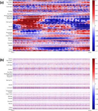
Figure 1 Time series (2013) of error (m) in 62-constituent harmonic prediction from (a) tide-and-surge ${\stackrel{\mathrm{̃}}{M}}_{\mathrm{s}}$ and (b) tide-only ${\stackrel{\mathrm{̃}}{M}}_{\mathrm{t}}$ models at estimating the tide-only model M_t. The vertical axis is a continuous line around the world coastline, starting and ending at Alaska via the eastern Pacific, Antarctica, western Atlantic, Arctic, eastern Atlantic, Indian Ocean, Australasia, and western Pacific. See Appendix A for a full explanation and reference map.

A significant source of error for this method is that a tide gauge is measuring the total water level, and hence the harmonic prediction $\stackrel{\mathrm{̃}}{G}$ includes all wave, steric, river levels, and surge effects. This is therefore not a prediction of the astronomical tide alone. Steric, wave, and river effects are omitted by the barotropic model, but M_s does include periodic radiational effects, which may be double-counted. We can test a minimum effect of this double-counting purely within the model by using ${\stackrel{\mathrm{̃}}{M}}_{\mathrm{s}}$, the harmonic prediction of the model including surge, as a proxy for the harmonics of the observations at gauges. Then the forecast procedure can be estimated as $M_r+{\stackrel{\mathrm{̃}}{M}}_{\mathrm{s}}$.

To estimate Δ, the error in this model forecast, we can once again use the model, assuming M_s≈G. Hence $\mathrm{\Delta }=M_{\mathrm{s}}-(M_r+{\stackrel{\mathrm{̃}}{M}}_{\mathrm{s}})=M_{\mathrm{t}}-{\stackrel{\mathrm{̃}}{M}}_{\mathrm{s}}$. That is, the minimum error from the current forecast procedure is equal to the error in the harmonic prediction from the model including surge at estimating the tide-only model; Fig. 1a. There are several striking features here, including annual cycles peaking around March in the Arctic, January in South East Asia, and June in Europe. Fortnightly cycles occur almost everywhere, with amplitudes of several centimetres. We will examine the causes of these below.

If it were possible to avoid the double-counting and provide astronomical tidal harmonics for the observations, the prediction would instead be equivalent to $M_r+{\stackrel{\mathrm{̃}}{M}}_{\mathrm{t}}$ and the error would become $\mathrm{\Delta }=M_{\mathrm{s}}-(M_r+{\stackrel{\mathrm{̃}}{M}}_{\mathrm{t}})$=$M_{\mathrm{t}}-{\stackrel{\mathrm{̃}}{M}}_{\mathrm{t}}$, as shown in Fig. 1b. Since we are using the model as a proxy for observations, if the harmonic prediction were an exact reproduction of the tide-only model then Δ=0. In practice Δ<5 cm at most UK sites and the monthly cycle has gone, but in the Bristol Channel there is still an error of around 50 cm, indicating that the 62 harmonic constituents are not capturing all of the model tide and further shallow-water constituents may be required. This is consistent with the conclusions of Flowerdew et al. (2010), who found an “average (across UK ports) RMS error (in harmonic prediction of a tide-only run) of 7 cm with a maximum value of 29 cm at Newport, in the Bristol Channel”, using 50 constituents on the CS3X model.

2.4 Fortnightly cycle arising from small changes to S₂ phase

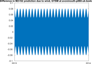
Figure 2 Fortnightly cycle of prediction change (metres) due to small changes in constituents M₂+S₂ alone based on Avonmouth. S₂ amplitude change 3.5 cm, phase change 3.5^∘, M₂ amplitude change 1 cm, phase change 0.2^∘.

M₂ has a period of 12.42 h and S₂ exactly 12 h. They move in and out of phase with each other twice in a lunar month, resulting in the spring–neap cycle. A small change in phase to the S₂ harmonic would result in a change of which days it is in phase with M₂ and hence a substantial change in total tidal amplitude at a given date. For example, near Avonmouth in the Bristol Channel, S₂ derived from M_s has an amplitude 3.5 cm greater than S₂ derived from M_t; however, there is a phase change of around 3.5^∘, so the tide arrives 7 min later. Figure 2 shows how this and smaller changes in M₂ account for differences between ${\stackrel{\mathrm{̃}}{M}}_{\mathrm{t}}$ and ${\stackrel{\mathrm{̃}}{M}}_{\mathrm{s}}$ of up to 5–8 cm on a fortnightly cycle between these limits. This can account for about half the error in forecasted high water at Avonmouth, which varies between 5 and 20 cm on a fortnightly cycle Byrne et al. (2017). Similar variation in error of the forecast was seen by Flowerdew et al. (2010).

2.5 Quantifying surge-forecasting error due to disregarding non-linearity

The forecasting approach of the linear addition of a non-linear model residual to a harmonic prediction, $F=M_r+\stackrel{\mathrm{̃}}{G}$, can also cause errors. Disagreements in phase between the model tide M_t and harmonic prediction from the gauge $\stackrel{\mathrm{̃}}{G}$ affect the forecast of an individual surge event.

Consider a simplified example in which the tide can be modelled by a single constituent, M_t=Acos(σt). Suppose there is a storm surge in which there is a uniform additional water level A_s and an advancement of the tide of t=δ, so the tide-and-surge model is $M_{\mathrm{s}}=A_{\mathrm{s}}+A\cos \left(\mathit{\sigma }\right(t+\mathit{\delta }\left)\right).$ As before, the model residual is given by $M_r=M_{\mathrm{s}}-M_{\mathrm{t}}$.

Suppose the harmonic prediction at the gauge agrees in amplitude to the tide-only model, but has slightly different phase: $\stackrel{\mathrm{̃}}{G}=A\cos \left(\mathit{\sigma }\right(t+\mathit{ϵ}\left)\right).$

The skew surge is defined as the difference between the maximum water level, here max(M_s), and $max\left(\stackrel{\mathrm{̃}}{G}\right)$. The error in the skew surge forecast is $E=max(M_r+\stackrel{\mathrm{̃}}{G})-max\left(M_{\mathrm{s}}\right)$. Substituting in and assuming phase changes are small, we find A_s cancels out and can show analytically that

$${\displaystyle }E\approx A\left(\cos \left(\mathit{\sigma }\mathit{ϵ}\right)-\cos \left(\mathit{\sigma }\right(\mathit{\delta }+\mathit{ϵ}\left)\right)+\cos \left(\mathit{\sigma }\mathit{\delta }\right)-\mathrm{1}\right).$$

This is illustrated in Fig. 3, with A=3 m, $\mathit{\sigma }=\mathrm{2}\mathit{\pi }/\mathrm{12.42}{\mathrm{h}}^{-\mathrm{1}}$ (M₂), and the surge advancing the tide by δ=30 min. The residual M_r is decreasing during high water due to the advanced tide. So if the observed harmonics have high water later than the model (ϵ=5 min), the forecast skew surge is underestimated by 3 cm. If the observed harmonics predict high water earlier than the model ($\mathit{ϵ}=-\mathrm{5}$ min), the forecast skew surge is overestimated by 3 cm.

Although in practice there are more constituents, a similar relationship will still hold in a small window about each high tide. Where there are frequent surges with a consistent effect on the tidal phase we would expect ϵ to have the same sign as δ, as the gauge registers water levels more like the tide-and-surge model than the tide-only model and the harmonic predictions would follow suit.

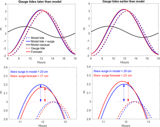
Figure 3 Suppose a surge adds a constant amplitude of 20 cm and also advances the underlying 3 m amplitude M₂ tide by a constant 30 min. If the harmonics of the observations differ in phase by 5 min from the model a forecast error of ±3 cm will result as shown. Lower panels are magnified to show high water.

3 The difference of specific harmonics

Figure 4 shows the vector difference in individual constituents between tide-and-surge and tide-only models run for 2013 along the coast globally. With some exceptions in the Arctic and Antarctic, the effect on S_a is around 5–20 cm, with around half that effect on S_sa, although in the Indian Ocean there is a change to S_a only. Since the model was only run for 1 year, S_a may not be representative of all years, but Fig. 4 indicates typical changes. In the Baltic, the seasonal change is wind forced, but elsewhere it is consistent with the annual and semi-annual cycles in sea-level atmospheric pressure (Chen et al., 2012).

MS_f is affected by the surge component, as a side effect of the interaction between M₂ and S₂. This is because MS_f is the fortnightly constituent which arises from the combination of M₂ and S₂, with a speed equal to the difference of their speeds. MS₄ is the counterpart to this, with a speed equal to the sum of the speeds of M₂ and S₂ (Pugh and Woodworth, 2014). Less explicable is the effect on M_m and M_f, but it may be due to insufficient separation with MS_f over a relatively short record. Another possibility is that non-tidal power in the tide-and-surge model is leaking into M_m and M_f estimates. Eliminating this would require a many-year model run.

The diurnal constituents K₁ and O₁ are affected by less than 5 cm and are only changed regionally in the Antarctic. S₁, however, is everywhere less than 0.1 cm in the tide-only model, but with the surge model peaks at 0.5 cm in northern Australia, the broadest regional effect being 0.2–0.3 cm in South East Asia, consistent with the findings of Ray and Egbert (2004).

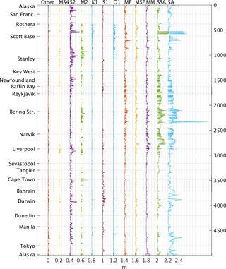
Figure 4 Vector difference (m, offset) between coefficients fitted to GTSM tide-and-surge (M_s) or tide-only (M_t) model. This is the breakdown into constituents of the difference between the panels of Fig. 1. The maximum effects for these harmonics and others are given in Table B1. See Fig. 1 and Appendix A for an explanation of coastal axis.

It may come as a surprise that constituents such as M₂, which has a purely lunar frequency, could possibly be affected by the weather. There is a very small atmospheric tide at M₂, peaking at the Equator at about 0.1 mbar (Schindelegger and Dobslaw, 2016). But more significant is the non-linear interaction of surge and tide. The surge may consistently advance the phase of the tide during low-pressure events and certain wind configurations. A high-pressure system could delay the phase of the tide, but there is asymmetry between these events, so there is a net bias on the phase when the weather is included.

The effect on higher-order constituents is everywhere less than 5 cm. The maximum difference in the UK and globally for each constituent is given in Appendix B. In the UK, the constituents affected the most by including the surge are S₂, S_sa, M₂, S_a, M_m, MS₄, MS_f, and M_f, with a maximum change of >2 cm, and a further 19 constituents change 1–2 cm. Globally, S_a and S_sa are far more significant, but S₂, M_f, M₂, M_m, MS_f, S₁, K₁, K₂, O₁, M_A2, and MS₄ all change more than 4 cm (somewhere on the global coast). A vector difference of 13 cm in S₂ is seen in north-west Australia.

We tested the stability of these results to the number of constituents fitted using the list of 115 harmonics usually associated with 18.6 years of data (see the Supplement) and found that the changes remain within 0.2 cm.

3.1 S₂ atmospheric tide

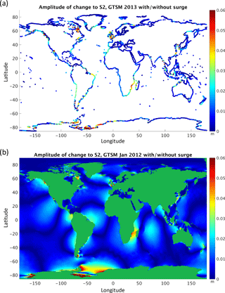
Some of the difference between the harmonics of surge and tide-only models is directly attributable to the atmospheric tides. The global atmospheric pressure field contains S₂ variations with an amplitude of about 1.25cos³ϕ mbar for latitude ϕ (Pugh and Woodworth, 2014). GTSM air pressure and wind forcing is taken from the ERA-Interim data set (Appendix A), and the ocean response to that forcing at S₂ is contained in the difference between the harmonic predictions of the M_s and M_t model runs (Fig. 5). It is consistent with response analysis based on the S₂ tides seen in ECMWF reanalysis data (Dobslaw and Thomas, 2005) and in a two-layer model forced by eight constituents (Arbic, 2005). The 6 h sampling prevents ERA-Interim forcing from capturing the S₂ atmospheric tide correctly (Dobslaw and Thomas, 2005), but the analysis in this paper is self-consistent with the forcing used.

Figure 5 Amplitude (m) of S₂ difference between coefficients fitted to the GTSM tide-and-surge (M_s) or tide-only (M_t) model. (a) Coastal data only, whole of 2013; (b) 26 primary coefficients fitted to January 2012 only.

4 Highest Astronomical Tide and Lowest Astronomical Tide

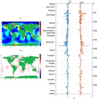
Figure 6 (a) Range calculated from maximum and minimum of 18.6-year prediction at 15 min intervals from 26 primary and 8 related constituents and nodal modulations derived from 1-month tide-only GTSM. (b) Difference between (a) and $\mathrm{2}({\mathbf{M}}_{\mathrm{2}}+{\mathbf{S}}_{\mathrm{2}}+{\mathbf{O}}_{\mathrm{1}}+{\mathbf{K}}_{\mathrm{1}})$ from the same run. (c)  Change in metres along the coast of predicted LAT (blue) and HAT (red, offset 1 m) between ${\stackrel{\mathrm{̃}}{M}}_{\mathrm{t}}$ and ${\stackrel{\mathrm{̃}}{M}}_{\mathrm{s}}$ (tide only or tide and surge). Tides derived from 62 constituents from GTSM 2013. See Appendix A for an explanation of coastal axis.

The Highest Astronomical Tide (HAT) is used internationally for flood-forecasting reference levels and in navigation for clearance under bridges. HAT can be used in structural design alongside skew surge as an independent variable for determining return-period water levels. The Lowest Astronomical Tide (LAT) is also an important parameter recommended for use as the datum on navigation charts (IHO, 2017). Once the phases and amplitudes A_n and g_n are known, $\stackrel{\mathrm{̃}}{G}\left(t\right)$ is fully determined by Eq. (1), and the future HAT and LAT are given by $\max \left(\stackrel{\mathrm{̃}}{G}\right(t\left)\right)$ and $\min \left(\stackrel{\mathrm{̃}}{G}\right(t\left)\right)$. But because of the overlap in phase of the forcing between the constituents and the f_n and u_n nodal modulations, it is not trivial to write HAT or LAT algebraically. They are therefore determined by inspection of the predicted tides, preferably over a 18.6-year nodal cycle. Figure 6a shows the range, HAT minus LAT, when we do this by synthesising a predicted tide at 15 min intervals over 18.6 years globally. Radiational effects are omitted from this figure, which is based on a tide-only run. Since the GTSM data were limited to 1 month, it uses only 34 constituents, therefore omitting S₁ and the long-period contributions to HAT and LAT.

An approximate calculation of range as $\mathrm{2}({\mathbf{M}}_{\mathrm{2}}+{\mathbf{S}}_{\mathrm{2}}+{\mathbf{O}}_{\mathrm{1}}+{\mathbf{K}}_{\mathrm{1}})$ is occasionally used (Yotsukuri et al., 2017), but the error due to this can be over 1 m (Fig. 6b). N₂ is a significant contributor, at about 20 % of M₂ in many sites worldwide. A few tens of centimetres are accounted for by the omission of the nodal modulations, and there are also the shallow-water constituents at the coast.

Figure 6c shows the effect on HAT and LAT of including surge in the GTSM. Coastal locations are shown and 62 constituents used. In many places around the world the HAT is higher when the tide-and-surge model is used. So the observation-based HAT has been raised by some radiational component. But in most of the UK, the HAT goes down when the tide-and-surge model is used to generate the tidal predictions. This is because the peak of the weather-related components does not coincide with the maximum astronomical effects alone. This implies that since the tide-gauge predictions include surge, the observation-based HAT in the UK is actually about 10 cm lower than true astronomical-only tidal height.

LAT tends to move the opposite way, so in most places the maximum tidal range is increased by using the tide-and-surge model. That is, the true astronomical-only tidal range is slightly less than that quoted from harmonics based on predictions. In Scotland (just above Liverpool in Fig. 6c) both LAT and HAT go down when the surge model is used to generate the tidal predictions, so the quoted LAT and HAT are actually about 10 cm lower than astronomical only.

The most extreme changes shown in Figure 6c are in the Arctic and Antarctic and should be interpreted with some caution as these areas are the least well represented in the model.

In places with small tide, seasonal signals may be dominant and they may be important to include for practical purposes. For example along the French–Italian coast from Mallorca to Sicily there is about a 7 cm increase in HAT and 3 cm decrease in LAT using the surge rather than tide-only model, so a highest “astronomical” tide based on predicted tide from observations actually contains about 7 cm due to seasonal winds.

5 Conclusions

There are substantial changes in tidal constituents fitted to tide-only and tide-and-surge model results. Even constituents with purely lunar frequencies, including M₂, may be affected by the surge, perhaps owing to asymmetry in phase changes of the tide under high- and low-pressure weather systems.

Some effects of the weather on tides are double-counted in the forecast procedure used in the UK, in which model residuals are added to gauge-based tide predictions. Even if the model were perfect, the minimum error from the current forecast procedure would be at least the error in the harmonic prediction including surge at estimating the tide-only model. If 62 constituents are fitted, this has a standard deviation of 20 cm at Avonmouth and 4–10 cm at most other UK gauges. 5–8 cm of the error at Avonmouth is due simply to a small change in phase of the S₂ harmonic. Further errors in total water level and skew surge arise directly from the linear addition of the harmonic prediction to the non-linear residual, particularly where there is a phase difference between model and gauge tidal harmonics.

Understanding and quantifying these errors is extremely important for forecasters, who will often need to advise or intervene on the expected surge risk, often based on a direct comparison between observed residuals and the forecast non-tidal residual. Where, for example, such a comparison may lead to the observed residual falling outside the bounds of an ensemble of forecast non-tidal residuals, forecasters may significantly (and potentially incorrectly) reduce their confidence in the model's estimate of surge if they are unaware of the additional errors associated with the harmonic tide and whether or not they have been addressed within the ensemble forecast's post-processing system. For comparison, across the UK tide-gauge network, short-range ensemble forecast RMS spread is of the order of 5–10 cm (Flowerdew et al., 2013). It is noted that, in the UK, the majority of coastal flood events occur around peak spring tides (Haigh et al., 2015), for which the sensitivity to any errors in the M₂–S₂ phase relationship is arguably at its highest.

The atmospheric tide at S₂ is present in the ERA-Interim forcing, and the ocean response to it, with an amplitude of about 1–5 cm, can be seen in the difference between the model results with and without surge. There is hence an argument for including an atmospheric tide forcing in a “tide-only” model, and this is being explored by Irazoqui Apecechea et al. (2018). In this case, care would need to be taken to omit the direct atmospheric tide forcing in the tide-and-surge version to avoid a different form of double-counting.

The estimates of the Highest and Lowest Astronomical Tide are influenced by radiational tides. HAT and LAT are most readily calculated by inspecting long time series of predicted tides, and if observation-based, these predictions will include weather-related components. In most places globally this results in HAT being calculated as higher than the strictly astronomical component and LAT being lower; however, the opposite is true in the UK. The effects are of the order of ∼10 cm.

For many practical purposes it is correct to include predictable seasonal and daily weather-related cycles in the HAT and LAT. However, the separate effects should be understood, as the radiational constituents may be subject to changing weather patterns due to climate change. It is also important not to double-count weather effects if HAT or LAT is used in combination with surge for estimating return-period water levels.

These considerations about HAT would also apply (proportionally less) to other key metrics such as mean high water.

Appendix A: Ordering of model sites around the coast

Figure A1 Sites used for analysis showing the order of coastal points (red to blue points shown above correspond to top to bottom in Figs. 1, 4, and 6).

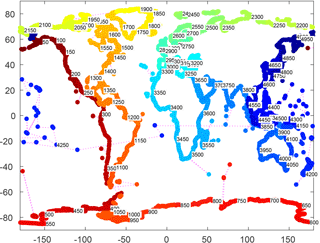
The coastal points in the model output are spaced roughly every 80 km and also wherever a tide gauge is situated, according to the GESLA data set (Woodworth et al., 2017). Due to automatic procedures to select output sites, a few may be incorrectly sited at model dry sites – these are clearly seen in plots as lacking sufficient high-frequency variability. The along-coast plots are ordered approximately from west to east around the world coastline, starting and ending at Alaska. The order is indicated in Fig. A1.

The algorithm for coastal order is as follows.

1. Define a single global coastline polygon.

   This is done using the GSHHG (Global Self-consistent, Hierarchical, High-resolution Geography) data set (Wessel and Smith, 1996) version gshhg2.3.6 (available at: https://www.ngdc.noaa.gov/, last access: 19 August 2016). We use the coarse resolution, with only Level 1 (coastline) and Level 6 (Antarctic Ice Shelf), although consistent results for this technique can be obtained including enclosed lakes. To merge the separate land masses and islands into a weakly simple polygon topologically equivalent to a disc, we start with a single land mass and add others in turn using pairs of identical edges as “bridges”. We start with the main land mass of Eurasia L₁ and find the closest vertex l to a vertex p from any of the remaining polygons [P₂,…P_N]. Suppose p belongs to polygon P_j. Then we add P_j to L₁ using two new edges $\overrightarrow{lp}$ and $\overrightarrow{pl}$ to give a new merged polygon L₂. The vertices of L₂ are then $\left[L_{\mathrm{1}}\right(\mathrm{1}:l),P_j(p:\mathrm{end},\mathrm{1}:p-\mathrm{1}),L_{\mathrm{1}}(l:\mathrm{end}\left)\right]$. Now repeat, searching for the nearest point in L₂ to any vertex in the remaining polygons $[P_{\mathrm{2}},\mathrm{\dots },P_{j-\mathrm{1}},P_{j+\mathrm{1}},\mathrm{\dots }{P}_N]$. It is necessary for all initial polygons to be defined in the same sense (anticlockwise). If inland seas (Level 2) are included, they should be defined clockwise. The GSHHG data are consistent with this definition. The distance for nearest points is defined as arc length on a sphere.

   This technique has the benefit of tending to group island chains together in a consistent order. It cannot produce crossing edges. Because polygons are added in distance order, islands near continents are added to their neighbouring coast, and remote mid-ocean islands tend to be clustered and attached to the nearest continent. The coasts of the Pacific, Atlantic and Indian, and Arctic Ocean are all treated clockwise. Antarctica is attached across the Drake Passage and ordered westward. Nearby locations across narrow islands (particularly Sumatra), isthmuses (Panama), and straits (Gibraltar) may be widely separated in the order. But neighbouring points in the order can be expected to have fairly smoothly varying oceanography, with the “bridges” often, although not necessarily, approximating shoals.

   As a final step we adjust the starting point of L₂ to be in Alaska for convenience of mapping.

2. Rank the coastal points according to the nearest point on the global polygon.

   Having defined this coastal order, we can apply it to any coastal data set, for example tide gauges. We number the vertices $[\mathrm{1},\mathrm{\dots },K]$. For each of the gauge locations T we find the nearest vertex k and then rank the gauges according to T_k. In the event of gauges being much closer than the resolution of the vertices, a quick method for refinement is to linearly interpolate with extra vertices along polygon edges. Some problems may also occur with islands not in the coarse-resolution data, which will tend to jump to the nearest coast.

   A further advantage here is that having defined the coastal polygon, the same order can be applied to different data sets and models, leading to closely comparable along-coast plots.

Appendix B: Tidal constituents

Table B1 lists the constituents used in this paper. For the 1-month model run, related constituents are used, and we fit 34 constituents with only 26 independent terms. 62 constituents are used for the 1-year run. The list of 115 usually applied to 18.6-year data is used only as a check on the stability of the result in Sect. 3 and is provided in the Supplement.

Table B1 Tidal harmonic constituents referred to in this paper and the maximum change constituents fitted to GTSM tide only (M_t) or with tide-and-surge forcing (M_s) at coastal locations, as from Fig. 4.