Comparative mesoscale eddy dynamics under geostrophic versus cyclogeostrophic balance from satellite altimetry

The curvature of streamlines plays a significant dynamical and structural role in meandering currents. At scales comparable to the deformation radius, the motion of eddies is governed by a balance between the pressure gradient force, the Coriolis force, and the centrifugal force. For mesoscale eddies, the nonlinear term induced by the local curvature of streamlines is non-negligible. This study compares the statistical and dynamical parameters of mesoscale eddies under geostrophic and cyclogeostrophic balances by examining five energetic North Pacific regions: the Aleutian Islands, Kuroshio Extension, South China Sea, California Coastal Current, and Hawaiian Islands. The comparison shows that cyclogeostrophic EKE is lower than geostrophic EKE for cyclonic eddies, whereas it is higher for anticyclonic eddies, particularly in energetic, low-latitude regions. The total number of eddies detected under the cyclogeostrophic balance is 35.65 % lower than under the geostrophic balance. However, the frequency distributions of eddy radii in both frameworks show a right-skewed normal distribution. Detection under the cyclogeostrophic balance tends to eddies with larger radii and shorter lifespans. The velocity difference between the two balances for eddies increases with decreasing latitude. Similarly, case studies indicate that anticyclonic eddies exhibit more pronounced variability in their energy evolution under the influence of streamline curvature, making them more prone to dissipation in low-latitude seas.

1 Introduction

Ocean currents serve as critical pathways for the transport of mass and energy in the global ocean, playing a central regulatory role in the Earth's climate system. Their variability is of fundamental importance to global climate change (Robert and Sebille, 2021). Curved flows are ubiquitous in the ocean. Centrifugal force arises in curved ocean flows due to curvature effects. Mesoscale and submesoscale meandering motions at the ocean surface satisfy cyclogeostrophic (CGEO) balance under the combined influence of centrifugal, pressure gradient, and Coriolis forces (Shakespeare, 2016; Cao et al., 2023). Eddies are a typical form of curved flow structure ubiquitous in the ocean. They play an indispensable role in oceanic circulation, heat budget, energy redistribution, biogeochemical transport, and global climate change (Dong et al., 2014). Furthermore, the generation mechanisms, and evolution of eddies are key to understanding changes in ocean stratification and circulation, providing crucial insights into the intrinsic dynamics of marine processes (Chelton et al., 2007; Dong et al., 2021; Yang et al., 2020). In each hemisphere of the Earth, cyclones rotate in the same direction as the planet's rotation (counterclockwise in the North, clockwise in the South), while anticyclones rotate in the opposite direction. Eddies cover a wide spectrum of horizontal scales, with radii ranging from several kilometers to hundreds of kilometers (Chelton et al., 2007; Chelton et al., 2011; Frenger et al., 2015; Tian et al., 2019). Those with a radius greater than or equal to the first baroclinic Rossby deformation radius (approximately 10–100 km) are classified as mesoscale eddies, while those with a radius smaller than 10 km but greater than the turbulent boundary layer scale (about 0.1–10 km) fall into the submesoscale category. Mesoscale eddies with coherent structures have longer lifespans and can persist in the ocean for several months to years, whereas smaller eddies are short-lived, typically lasting only from hours to a few days (Puillat et al., 2002; Ioannou et al., 2017; Laxenaire et al., 2018).

The North Pacific, with its complex circulation structure, is a region of highly active mesoscale eddies. It hosts intricate current systems such as the North Equatorial Current, the Kuroshio, and the North Pacific Current, where interactions between different flow systems generate a large number of mesoscale eddies. Previous studies have identified two zonal bands with high eddy kinetic energy in this region: one is the Kuroshio Extension, and the other is the North Pacific Subtropical Countercurrent region (Kang et al., 2010; Chang and Oey, 2014). In the Kuroshio Extension, eddy activity levels are modulated by the dynamical state of the Kuroshio and influenced by the wind stress curl in the eastern North Pacific. Both the Kuroshio and regional eddy intensity exhibit significant decadal oscillations (Qiu and Chen, 2005, 2013; Taguchi et al., 2010). The northern part of the Kuroshio Extension is dominated by anticyclonic eddies, while the southern part is predominantly cyclonic (Itoh and Yasuda, 2010). The North Pacific Subtropical Countercurrent region features complex circulation due to vertical shear with the North Equatorial Current, leading to intense mesoscale eddies. Previous studies have completed eddy identification (Hwang et al., 2004) and dataset construction (Liu et al., 2012) in this area, confirming that eddies intensify as they propagate westward and influence the Kuroshio. Eddy kinetic energy in this region also exhibits interannual scale characteristics (Qiu and Chen, 2010, 2013; Chow et al., 2017), with baroclinic instability being a key driver of its seasonal variability (Chang and Oey, 2014). Additionally, the spatiotemporal variability of eddies is regulated by baroclinic instability (Travis and Qiu, 2017; Rieck et al., 2018). The Hawaiian Islands region is recognized as an area of frequent eddy occurrence (Calil et al., 2008). Using available datasets of sea surface height, sea surface temperature, and surface wind stress, Yoshida et al. (2011) further investigated the interannual-to-decadal variability of eddies within the Hawaiian Lee Countercurrent (HLCC) band. The spatiotemporal resolution of northeasterly trade winds and regional wind forcing significantly influences the distribution of eddy kinetic energy in this area (Calil et al., 2008). In the California Current System, eddies frequently form near capes, islands, and regions with sharp topographic variations (Dong et al., 2012; Kurczyn et al., 2012).

Satellite altimetry has played an indispensable role in research areas such as the observation of mesoscale oceanic eddies (Chelton et al., 2007; Andres et al., 2008).The application of satellite altimetry data (e.g., AVISO/CMEMS) under the geostrophic (GEO) balance has enabled considerable progress in identifying and tracking eddies, as well as analyzing their dynamical characteristics. However, because geostrophic theory neglects the contribution of centrifugal forces in actual ocean flow, altimeter-derived sea surface velocities often exhibit biases in curved flow regions under the geostrophic balance assumption (Uchida et al., 1998; Fratantoni, 2001; Uchida and Imawaki, 2003; Douglass and Richman, 2015; Cao et al., 2023). These biases are distinct from the ageostrophic velocity components induced by surface wind stress, and it is mainly caused by the nonlinear term induced by the local curvature of the streamline. Cyclogeostrophic balance have demonstrated superior performance in characterizing eddy dynamics in certain regional seas, such as the Gulf Stream, the Kuroshio Extension, the intense eddy zone in the Mozambique Channel, and the Mediterranean Sea (Fratantoni, 2001; Uchida and Imawaki, 2003; Penven et al., 2014; Ioannou et al., 2019). Although a wealth of findings has been accumulated in previous studies, little has been reported regarding the practical implementation of this cyclogeostrophic framework in complex and variable current environments like the North Pacific. In terms of theoretical application, the limitations of geostrophic balance theory lead to distorted representations of eddy dynamic characteristics in the complex and variable flow environment of the North Pacific. Meanwhile, systematic studies on the application of cyclogeostrophic balance theory in this region remain scarce, particularly in comprehensively comparing different types of eddies under both balance regimes. Using the global surface cyclogeostrophic current dataset corrected by Cao et al., 2023 based on the latest version of AVISO satellite altimetry data, this study compares eddy characteristics in the North Pacific between this refined dataset and the original altimetry product. Through quantitative diagnostic analysis, we aim to clarify the mechanism by which curvature influences the dynamic processes of surface flow fields. The structure of this paper is as follows: Section 2 presents the methods and data employed in the study. In Sect. 3, we examine the statistical characteristics of kinematic parameters, the differences in dynamical parameters of mesoscale eddies under cyclogeostrophic and geostrophic balance, as well as the contrasting dynamical processes of individual eddies between the two balances, are summarized in Sect. 4.

2 Materials and Methods

2.1 Remote sensing data

The geostrophic current velocity fields were derived from the National Centre for Space Studies (CNES; French: Centre National D'Études Spatiales)'s Archiving Validation and Interpolation of Satellite Oceanographic (AVISO). This product synthesizes data from multiple satellite missions, including TOPEX/Poseidon, Jason-1, ERS, Envisat, and others, processed through the Data Unification and Altimeter Combination System (DUACS). This study utilizes the AVISO DT 2018 dataset, which has a daily temporal resolution and a spatial resolution of 0.25°×0.25°, covering the period from 1 January 1993–31 December 2018. The data URL is provided in the Code, data, or code and data availability section.

The cyclogeostrophic current data employed in this study were derived from the geostrophic currents calibrated by Cao et al. (2023). This dataset accounts for the influence of eddy curvature and was generated by applying an iterative method to perform cyclogeostrophic correction on 26 years of global surface geostrophic currents from the AVISO product.

2.2 Cyclogeostrophic balance equations

In the context of an horizontal, stationary, and inviscid flow, the momentum equation which links SSH and surface horizontal currents U is

$$\begin{array}{}\text{(1)}& U\cdot \mathrm{\nabla }U+f\mathit{k}\times U=-g\mathrm{\nabla }\mathit{\eta }\end{array}$$

where f is the Coriolis parameter, k is a vertical unit vector, η and g are the sea surface height and gravitational acceleration parameter, respectively. For Mesoscale curved ocean currents, the nonlinear term induced by the local curvature of the streamline cannot be ignored. Introducing the geostrophic velocities U_g from Eq. (1), this equation can be transformed to the form

$$\begin{array}{}\text{(2)}& \mathit{U}-{\displaystyle \frac{\mathit{k}}{f}}\times (\mathit{U}\cdot \mathrm{\nabla }\mathit{U})={\mathit{U}}_{\mathrm{g}}\end{array}$$

In cylindrical coordinates, this equation simplifies for the azimuthal velocities to the gradient wind equation (Knox and Ohmann, 2006):

$$\begin{array}{}\text{(3)}& {\displaystyle \frac{V^{\mathrm{2}}}{fR}}+V=V_{\mathrm{g}}\end{array}$$

where V is the azimuthal velocity, V_g is the geostrophic velocity derived from the pressure gradient, and R is the radius of curvature. This equation admits an analytical solution for V.

According to Eq. (3), the cyclogeostrophic Rossby number can be given by:

$$\begin{array}{}\text{(4)}& {\text{Ro}}_{\mathrm{c}}={\displaystyle \frac{V}{fR}}={\displaystyle \frac{V_{\mathrm{g}}-V}{V}}\end{array}$$

Analysis shows that the discrepancies between geostrophic and cyclogeostrophic currents are governed by curvature:

$$\begin{array}{}\text{(5)}& \mathit{\kappa }={\displaystyle \frac{f(V_{\mathrm{g}}-V)}{V^{\mathrm{2}}}}\end{array}$$

where, κ is the curvature.

2.3 Kinematic and dynamic parameters

The eddy kinetic energy (EKE) is computed at each point in space and time as

$$\begin{array}{}\text{(6)}& \text{EKE}={\displaystyle \frac{\mathrm{1}}{\mathrm{2}}}\times \left[\right(u^{\prime }{)}^{\mathrm{2}}+\left(v^{\prime }{)}^{\mathrm{2}}\right]\end{array}$$

where u^′ and v^′ are the surface velocity anomalies of zonal and meridional currents. The geostrophic eddy kinetic energy is obtained by the current components computed from the sea surface height anomalies (SSHA) of AVISO/DUCAS. For each component, the calculations are as follows:

$$\begin{array}{}\text{(7)}& {\displaystyle }& {\displaystyle }{u}^{\prime }=-{\displaystyle \frac{g}{f}}\left({\displaystyle \frac{\partial h^{\prime }}{\partial y}}\right)\text{(8)}& {\displaystyle }& {\displaystyle }{v}^{\prime }={\displaystyle \frac{g}{f}}\left({\displaystyle \frac{\partial h^{\prime }}{\partial x}}\right)\end{array}$$

where h^′ is the SSHA. The cyclogeostrophic eddy kinetic energy is obtained by the cyclogeostrophic surface currents.

The normalized difference between climatic mean geostrophic EKE and cyclogeostrophic EKE is given by:

$$\begin{array}{}\text{(9)}& \begin{array}{rl}{\displaystyle }& {\displaystyle }{a}_{\text{EKE}}={\displaystyle \frac{\stackrel{\mathrm{‾}}{{\text{EKE}}_i}-\stackrel{\mathrm{‾}}{{\text{EKE}}_{\mathrm{g}}}}{\stackrel{\mathrm{‾}}{{\text{EKE}}_{\mathrm{g}}}}}\\ {\displaystyle }& {\displaystyle }={\displaystyle \frac{{\sum }_{i=\mathrm{1}}^n\frac{\mathrm{1}}{\mathrm{2}}\left((u_i^{\prime }{)}^{\mathrm{2}}+(v_i^{\prime }{)}^{\mathrm{2}}\right)-{\sum }_{i=\mathrm{1}}^n\frac{\mathrm{1}}{\mathrm{2}}\left((u_{\mathrm{g}}^{\prime }{)}^{\mathrm{2}}+(v_{\mathrm{g}}^{\prime }{)}^{\mathrm{2}}\right)}{{\sum }_{i=\mathrm{1}}^n\frac{\mathrm{1}}{\mathrm{2}}\left((u_{\mathrm{g}}^{\prime }{)}^{\mathrm{2}}+(v_{\mathrm{g}}^{\prime }{)}^{\mathrm{2}}\right)}}\\ {\displaystyle }& {\displaystyle }\times \mathrm{100}\mathit{\%}\end{array}\end{array}$$

where EKE_i denotes the EKE of the cyclogeostrophic surface currents, EKE_g represents the EKE of the geostrophic surface currents. $u_i^{\prime }$, $v_i^{\prime }$ are the zonal and meridional velocity anomalies of the cyclogeostrophic surface currents, respectively, while ug^′ and vg^′ denote the corresponding velocity anomalies of the geostrophic surface currents.

Enstrophy is defined in fluid dynamics as half the square of the vorticity (Weiss, 1991). It serves as a key dynamical parameter that quantifies the local concentration of rotational intensity or eddy strength in the current. On each grid cell, the eddy enstrophy is given by:

$$\begin{array}{}\text{(10)}& \text{ENS}={\displaystyle \frac{\mathrm{1}}{\mathrm{2}}}{\left({\displaystyle \frac{\partial v^{\prime }}{\partial x}}-{\displaystyle \frac{\partial u^{\prime }}{\partial y}}\right)}^{\mathrm{2}}\end{array}$$

where the x and y axis represent the zonal and meridional lengths of the grid point.

Similarly, the strain rate, which characterizes the deformation of the flow field, manifests as stretching in one direction and compression in the perpendicular direction. This continuous stretching and contracting in horizontal space disrupts the geostrophic balance of the flow (McWilliams, 2006; Zhang et al., 2019). The strain rate S is composed of both shear $\mathit{\vartheta }=\partial v^{\prime }/\partial x+\partial u^{\prime }/\partial y$ and stretching deformation $\mathit{\varsigma }=\partial u^{\prime }/\partial x-\partial v^{\prime }/\partial y$ components and is expressed as:

$$\begin{array}{}\text{(11)}& S=\sqrt{{\mathit{\vartheta }}^{\mathrm{2}}+{\mathit{\varsigma }}^{\mathrm{2}}}\end{array}$$

The relative vorticity, which quantifies the rotational characteristics of an eddy, can be expressed as follows:

$$\begin{array}{}\text{(12)}& \mathit{\zeta }={\displaystyle \frac{\partial v^{\prime }}{\partial x}}-{\displaystyle \frac{\partial u^{\prime }}{\partial y}}\end{array}$$

The eddy Rossby number, which is related to the maximum eddy radius (R_max) and velocity (V_max), is calculated by:

$$\begin{array}{}\text{(13)}& Ro={\displaystyle \frac{V_{max}}{f{R}_{max}}},\end{array}$$

2.4 Eddy Automated Detection Algorithm

Eddies are defined as coherent fluid regions in which velocity vectors rotate cyclonically or anticyclonically about a central point. Automated eddy detection methods can be broadly categorized into Eulerian and Lagrangian approaches, depending on the type of underlying data (Nencioli et al., 2010). Within the Eulerian framework, eddies are typically identified from two- or three-dimensional flow field representations. In contrast, the Lagrangian approach detects eddies by tracking fluid particle trajectories. In this study, a Eulerian eddy-detection algorithm is employed, which has been successfully applied to eddy identification in global oceans (Dong et al., 2022). The center of an eddy is determined based on the geometry of velocity vectors through four constraints:

1. Along the east–west direction through the eddy center, the surface velocity anomalies of the meridional flow exhibit opposite signs on either side of the center and increase gradually away from it;

2. Along the north–south direction through the eddy center, the surface velocity anomalies of the zonal flow show opposite signs on either side of the center and increase gradually away from it;

3. The velocity magnitude reaches a local minimum in the vicinity of the eddy center;

4. Around the eddy center, the rotation of the velocity vectors is consistent. The directions of two adjacent velocity vectors must lie within the same or two adjacent quadrants.

The constraints require the specification of two parameters: parameter a applies to the first, second, and fourth constraints, while parameter b corresponds to the third constraint. Parameter a defines the spatial range, expressed in number of grid points, over which the increase in the magnitude of v along the east–west axis and of u along the north–south axis is examined. It also specifies the closed contour around the eddy center along which changes in the direction of velocity vectors are evaluated. Parameter b determines the size of the region, also measured in grid points, that is used to identify the local velocity minimum (Nencioli et al., 2010). To ensure global applicability, the parameters are set to a=4 and b=3 based on empirical optimization. Moreover, ,the minimum velocity detected by the first three constraints is not necessarily related to the eddy structure and cannot be directly defined as the eddy center. Therefore, the fourth constraint must be introduced to prevent false detection.

3 Results and Discussion

3.1 Eddy Kinetic Energy

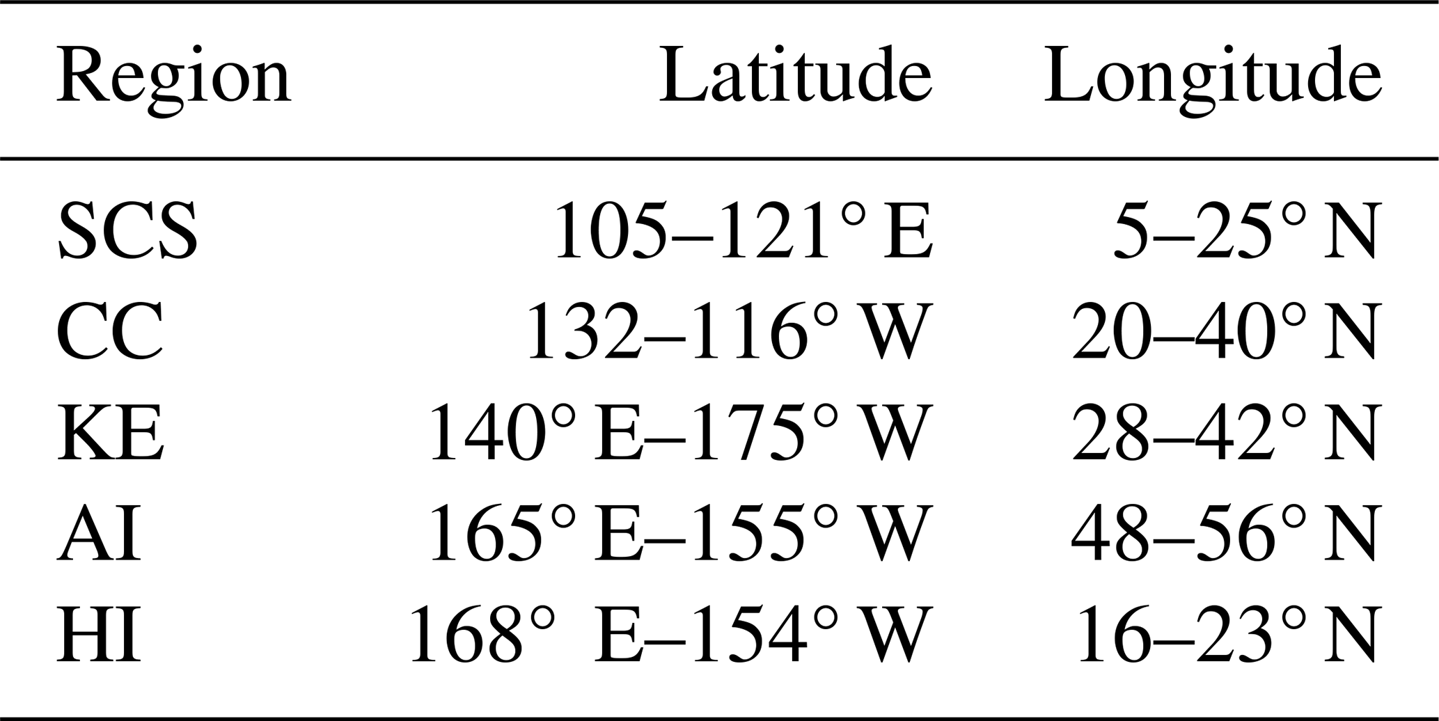
The EKE is an important parameter for characterizing eddy activity and serves as a key indicator for understanding the multi-scale dynamics of eddies. Cao et al. (2023) demonstrated that EKE after cyclogeostrophic adjustment exhibits marked differences across three distinct marine environments: low-latitude regions, eddy-rich zones with intense eddy-eddy interactions, and strongly curved frontal systems. Figure 1a depicts the spatial distribution of the normalized difference between the multi-year mean geostrophic and cyclogeostrophic EKE in the North Pacific from January 1993–December 2018. Based on this spatial pattern, five regions exhibiting the most pronounced differences were selected for detailed analysis: the South China Sea (SCS), the California Coastal Current (CC) region, the Kuroshio Extension (KE), the Aleutian Islands (AI), and the Hawaiian Islands (HI). The precise geographical boundaries of these regions are provided in Table 1.

Table 1 Location information of the selected research area.

The most pronounced differences occur in the KE and SCS regions. In the KE region, a significant difference in the EKE is observed across the main axis of the current. This is primarily attributed to western boundary intensification, which leads to higher velocities in this area. As shown in Eq. (5), the greater the velocity of the meandering current, the more pronounced the cyclogeostrophic effect becomes. In the SCS region, factors such as complex topography and Kuroshio intrusions contribute to abundant eddy activity (Lin et al., 2015; Zhang et al., 2016). Additionally, the weaker Coriolis force in this region leads, according to Eq. (5), to a more significant cyclogeostrophic correction effect. Driven by the combined effects of the Coriolis force and prevailing wind belts, the North Pacific Subtropical Gyre exhibits basin-wide cyclonic circulation. Within this gyre, the CC region shows a notable prevalence of cyclonic eddies among long-lived surface eddy populations (Kurian et al., 2011). Along its southern boundary, where currents flow southward, the EKE difference ratio is negative, notably reaching approximately −5 % in the CC region. In contrast, the Subpolar Gyre demonstrates anticyclonic circulation. Influenced by the Alaska Current, the AI region shows an EKE difference percentage around 10 %. In the HI region, due to wind stress curl and current shear in the eastern area (Dong et al., 2009), which enhance flow curvature and velocity gradients, the limitation of the geostrophic balance becomes more pronounced. Consequently, positive differences are distributed in the west while negative differences appear in the east, both with magnitudes around ±5 %.

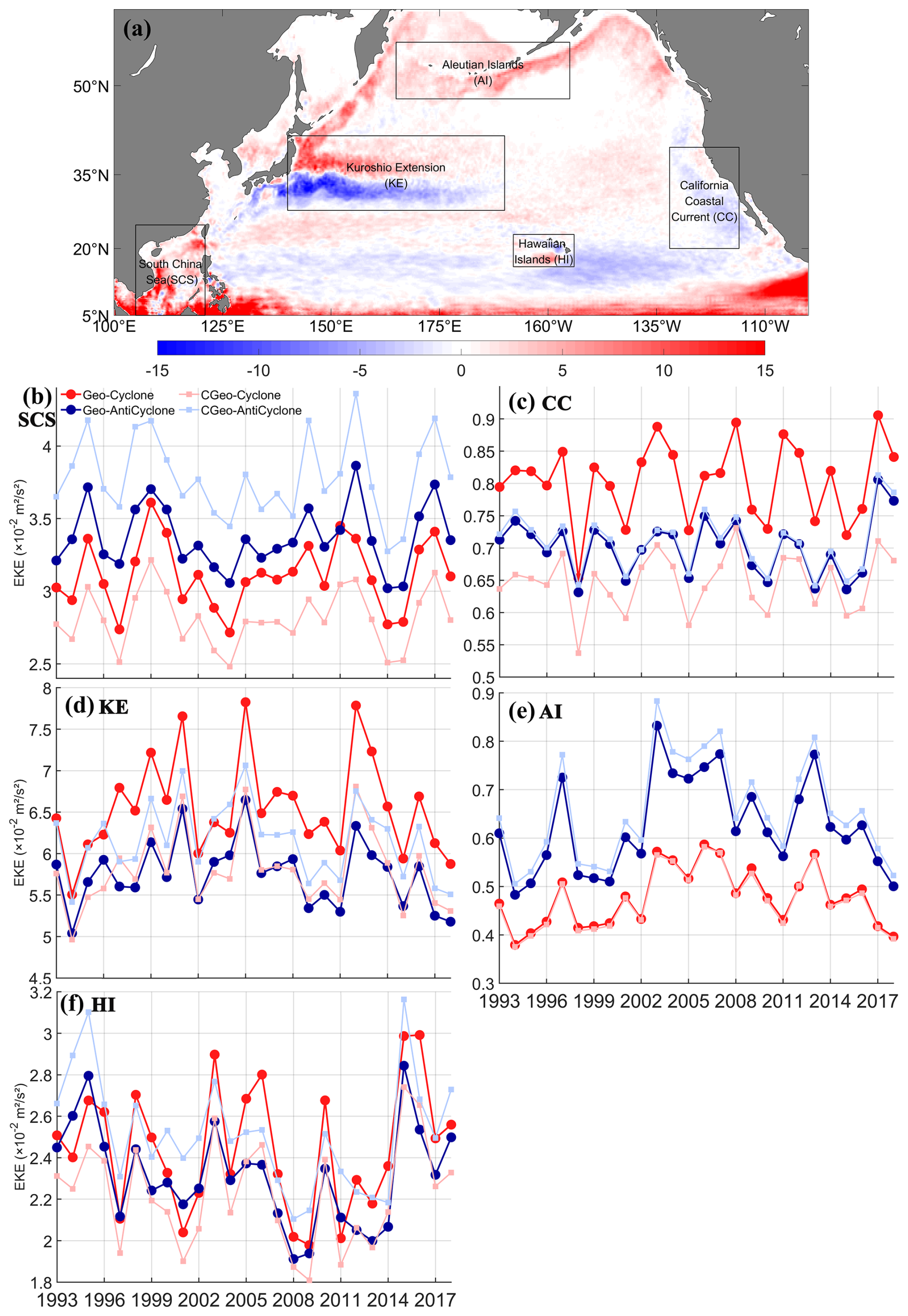
Figure 1 (a) Spatial distribution of normalized difference between multi-year average geostrophic EKE and cyclogeostrophic EKE over the period of January 1993–December 2018 in the North Pacific. Time series of interannual variation of area averaged EKE in the (b) South China Sea (SCS), (c) California Coastal Current (CC), (d) Kuroshio Extension (KE), (e) Aleutian Islands (AI), (f) Hawaii Islands (HI), the dotted solid blue and red lines represent geostrophic cyclonic and anticyclonic currents, respectively. The dotted solid light blue and red lines represent the cyclogeostrophic cyclonic and anticyclonic currents, respectively.

Figure 1b illustrates the interannual variability of EKE in the South China Sea (SCS) region. Geostrophic EKE derived from altimetry overestimates actual EKE in cyclonic eddies and underestimates it in anticyclonic eddies. Correspondingly, the geostrophic EKE exceeds the cyclogeostrophic value for cyclonic eddies by an annual mean of 9.69 %, while for anticyclonic eddies it is lower by 12.28 %. Temporally, the cyclogeostrophic correction proves more large for anticyclonic eddies. Spatially, the difference in this region are predominantly positive, indicating that the cyclogeostrophic current estimates exceed the geostrophic ones over most of the region. In the CC region (Fig. 1c), the average geostrophic EKE for cyclonic and anticyclonic eddies is 80.4 and 70.2 cm² s⁻², respectively, while the average cyclogeostrophic EKE values are 64.7 and 70.9 cm² s⁻². In the KE region (Fig. 1d), the geostrophic EKE of cyclonic eddies is higher than the cyclogeostrophic EKE, whereas the opposite is true for anticyclonic eddies. The annual mean difference is −11.47 % for cyclonic eddies and 7.21 % for anticyclonic eddies. In the AI region (Fig. 1e), differences in EKE between cyclonic and anticyclonic eddies under geostrophic and cyclogeostrophic balances are relatively small. This is primarily because the larger Coriolis force in high-latitude regions results in a smaller Rossby number under the cyclogeostrophic balance (Eq. 4), leading to an insignificant difference between the cyclogeostrophic and geostrophic flow velocities. The geostrophic EKE of cyclonic eddies exceeds the cyclogeostrophic EKE, with an annual mean difference of −0.93 %. For anticyclonic eddies, the geostrophic EKE is lower, yielding an annual mean difference of 5.10 %. Figure 1f presents the relative differences between cyclogeostrophic and geostrophic EKE over time in the HI region. The geostrophic EKE of cyclonic eddies is higher than the cyclogeostrophic EKE, while the reverse occurs for anticyclonic eddies. The mean difference is −9.17 % for cyclonic and 8.86 % for anticyclonic eddies.

To quantify the effect of the cyclogeostrophic correction on EKE, we normalized the average EKE and eddy lifetimes within eddy boundaries for two datasets in the study area. By applying this normalization, we can track how EKE changes over the eddy's full lifetime, as shown in Fig. 2. Across the five regions, the average normalized EKE exhibits a concave trend over the normalized eddy lifespan, first increasing and then decreasing. This reflects the typical evolution of energy during the development, maturity, and decay stages of eddies. However, differences exist among various regions and eddy types in terms of the amplitude of changes and the position of peaks. In the SCS region (Fig. 2a), the normalized cyclogeostrophic EKE of cyclonic eddies consistently exceeds the geostrophic EKE throughout their entire lifecycle, with opposing trends in growth and decay rates across different phases. For anticyclonic eddies, the variation in cyclogeostrophic EKE is smaller, and dissipation occurs more slowly during the decay phase. In the CC region (Fig. 2b), the differences in EKE between the two balances are relatively small during both the generation and decay stages. Under cyclogeostrophic balance, the EKE of cyclonic and anticyclonic eddies is more similar, and decay proceeds more gradually. In the KE region (Fig. 2c), the EKE of cyclonic eddies is comparable under both balances, whereas for anticyclonic eddies, the EKE difference is larger during the generation phase, and cyclogeostrophic EKE is better preserved during decay. Figure 2d shows that EKE in the AI region exhibits similar peaks and trends under the two balance frameworks, yet clear differences emerge during the decay phase. In the HI region (Fig. 2e), cyclonic eddies exhibit higher normalized cyclogeostrophic EKE in the generation phase, though the growth rate is lower, and the decline is faster during the mature and decay phases. During the formation and decay phases of eddies, when radii are often small, streamline curvature plays an enhanced role as described by the gradient-wind formula. However, the difference compared to eddies detected by the original altimeter data is not particularly pronounced. This could be influenced by the detection method inadvertently missing small radii eddies (You et al., 2022).

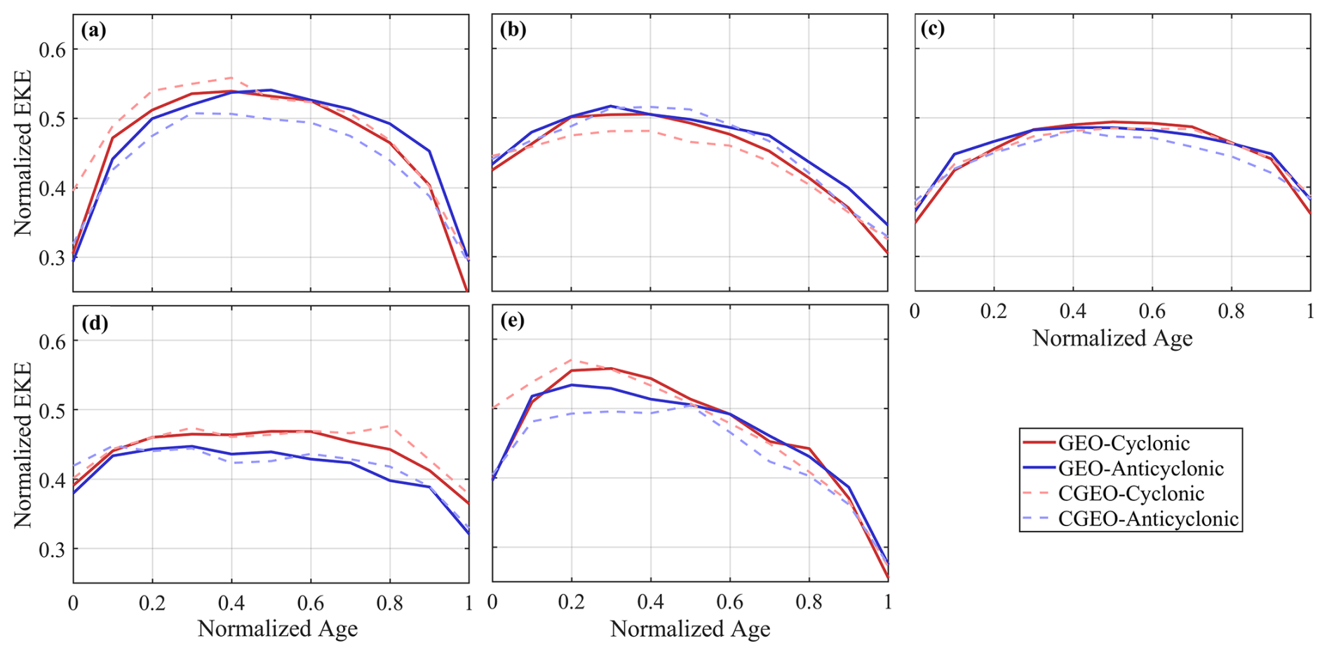
Figure 2 Temporal evolution of normalized eddy kinetic energy in (a) SCS, (b) CC, (c) KE, (d) AI, and (e) HI. Analysis restricted to eddies persisting>28 d. Solid red line represents geostrophic cyclonic eddies and dashed red line represents cyclogeostrophic cyclonic eddies. The solid and dashed blue lines indicate geostrophic and cyclogeostrophic anticyclonic eddies, respectively. Each life stage is defined by normalized age: generation ($\sim \mathrm{0}-\mathrm{0.1}$), intensification ($\sim \mathrm{0.1}-\mathrm{0.3}$), maturation ($\sim \mathrm{0.3}-\mathrm{0.8}$), and decay (>0.8).

3.2 Eddy Spatiotemporal Distributions, Sizes and Lifespan

An analysis and comparison of the number, radius, and lifespan of eddies (with lifespans exceeding 4 weeks) were carried out across five study regions in the North Pacific between 1993 and 2018. The Lagrangian method was applied to quantify eddy counts by treating each complete eddy lifecycle as a single unit. In terms of eddy numbers (Fig. 3a), the total under cyclogeostrophic balance is generally lower than that under geostrophic balance. Specifically, the geostrophic balance yields approximately 35.65 % more eddies than the cyclogeostrophic balance, which is far larger than the eddy count difference of about 8 % induced by different eddy detection algorithms (You et al., 2022). In the AI and KE regions, anticyclonic eddies predominate over cyclonic eddies, while in the CC and HI regions, cyclonic eddies are more prevalent than anticyclonic eddies. To gain a clearer understanding of the distribution of eddies in different regions, a 1°×1° grid was used to delineate the statistical areas. The counted eddies were confined to those with their entire lifecycle within the study area. Based on the center position of each eddy at each moment, all eddies within each grid point were counted. Compared to the geostrophic conditions (Fig. 3b and c), fewer eddies were detected under cyclogeostrophic conditions (Fig. 3d and e). Despite this difference, both frameworks show strong spatial correspondence across all regions. In the AI region, eddy occurrence is relatively sparse near the central coastal margin, whereas higher concentrations are observed in the northwestern and southeastern areas. The KE region exhibits a substantial number of eddies under both geostrophic and cyclogeostrophic conditions, with cyclonic eddies dominating the southern and eastern zones, and anticyclonic eddies more frequent in the northern and southwestern sectors. West of the Hawaiian Island, a localized area shows a notable density of eddies in both GEO and CGEO datasets. The CC is one of the most productive eastern boundary upwelling systems and exhibits frequent mesoscale activity. However, due to the predominance of cyclonic circulation in this region, the number of cyclogeostrophic eddies is relatively lower than that of geostrophic eddies.

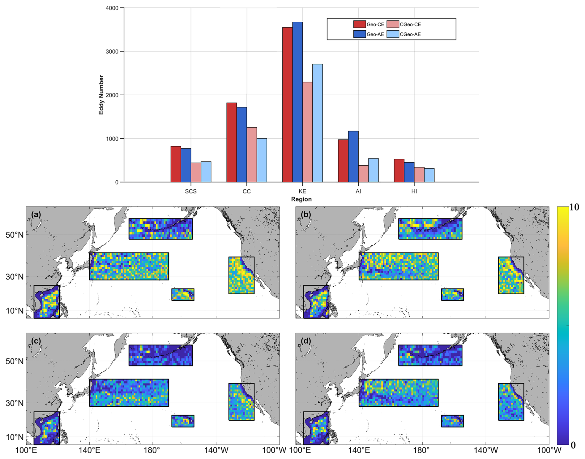
Figure 3 Comparison of eddy numbers. (a) Histograms of eddy numbers across the five study regions in the North Pacific. Geo-CE and Geo-AE denote geostrophic cyclonic and anticyclonic eddies, respectively; CGeo-CE and CGeo-AE indicate cyclogeostrophic cyclonic and anticyclonic eddies. (b–c) Spatial distributions of GEO-CE and GEO-AE. (d–e) Spatial distributions of CGEO-CE and CGEO-AE within the North Pacific study regions.

Regarding the average lifespan of eddies, the number of eddies with a lifespan of at least 4 weeks is shown in Fig. 4a. The average eddy lifespan under cyclogeostrophic conditions is shorter than under geostrophic conditions, with a difference of approximately 10 d in the Kuroshio Extension (KE) and California Current (CC) regions. The average lifespans under the two balance conditions are most similar in the South China Sea (SCS). Except in the CC region, the average lifespan of anticyclonic eddies is longer than that of cyclonic eddies in the other four regions. As for the average eddy radius (Fig. 4b), cyclogeostrophic eddies are generally larger than geostrophic eddies. A notable difference in average radius is observed between anticyclonic eddies (AE) and cyclonic eddies (CE) – under cyclogeostrophic conditions, both types exhibit a larger average radius compared to those under geostrophic conditions.

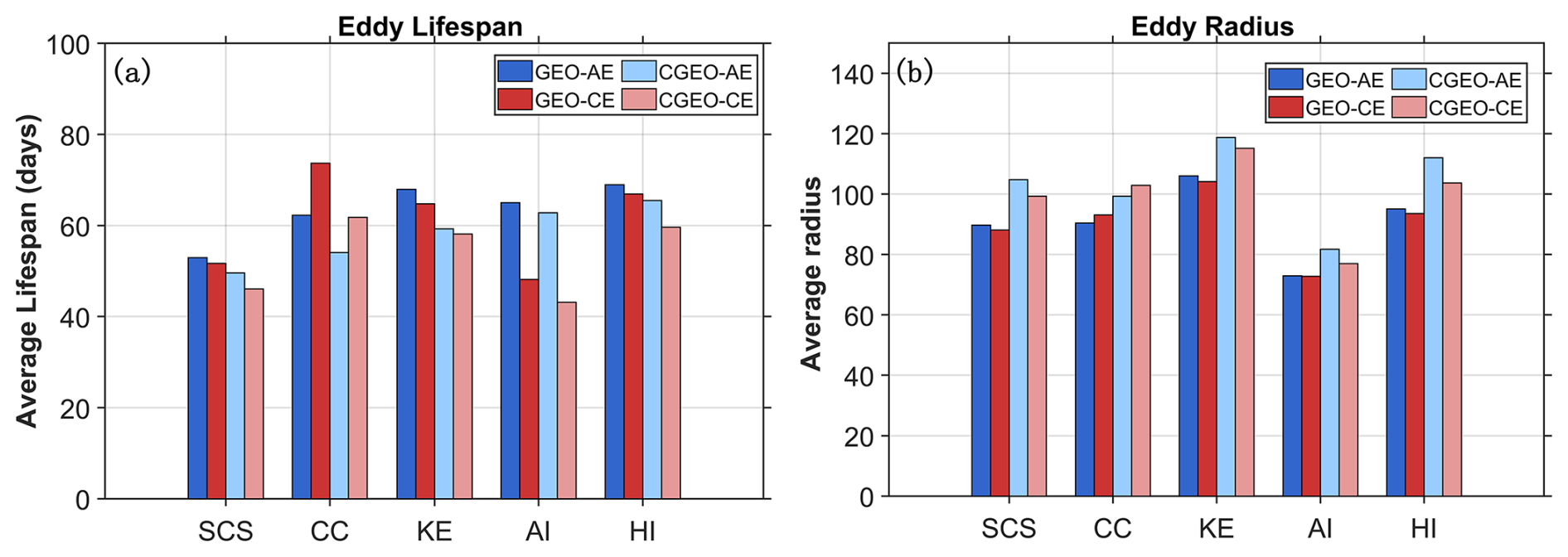
Figure 4 Statistics of (a) eddy lifespans (lifetime ≥ 4 weeks) and (b) radii across the five study regions in the North Pacific.

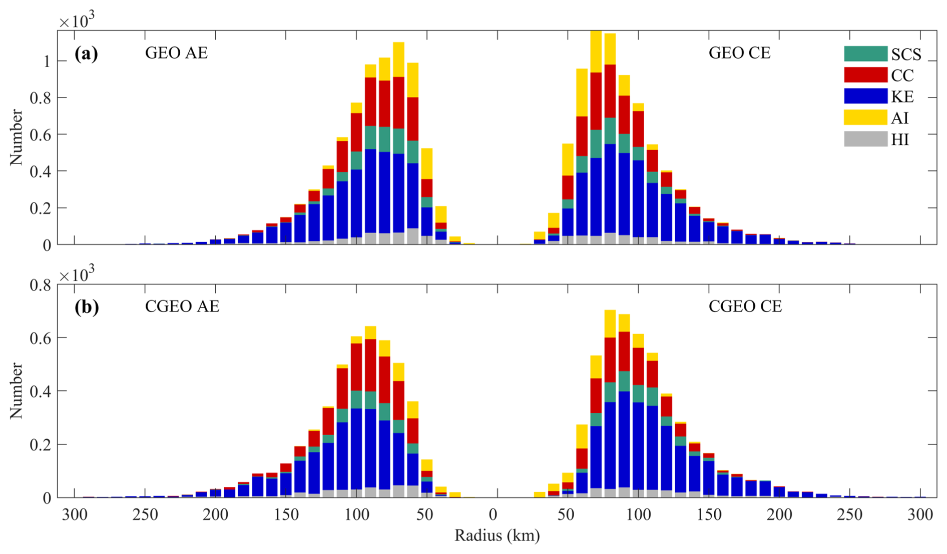
Figure 5 displays the distribution of eddy radii, showing a consistent right-skew across both datasets from the five regions. Eddy radii derived under the CGEO framework are generally larger than those under the GEO framework. In the CGEO dataset, cyclonic eddies (CE) with radii between 50–100 km comprise 57.5 % of the total, and anticyclonic eddies (AE) account for 56 %. In contrast, the GEO dataset shows higher proportions in this size range, with 65 % for CE and 63.2 % for AE, indicating a greater abundance of small-radius eddies. The presence of more larger and longer-lived eddies in the KE region is mainly caused by baroclinic instability, which induces meandering in the KE path (Ji et al., 2018).

Figure 5 Histograms of eddy radius for the (a) GEO and (b) CGEO datasets.

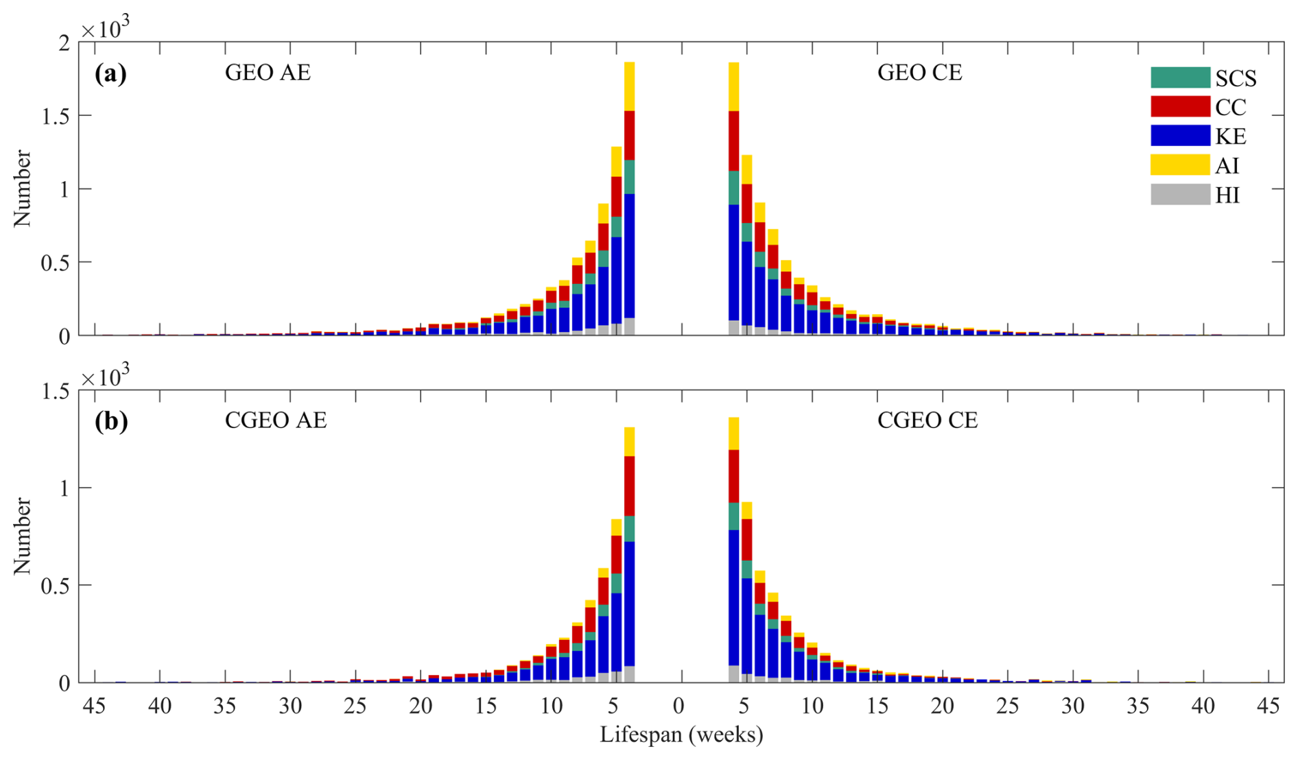
Statistical analysis of eddy lifespans (Fig. 6) reveals that short-lived eddies are more numerous than long-lived eddies in both datasets. As lifespans increase, the numbers of both anticyclonic eddies (AEs) and cyclonic eddies (CEs) decrease. This occurs because the rotational energy of an eddy gradually lost to the surrounding environment through various processes after its formation. Consequently, eddies with longer lifespans become increasingly difficult to maintain, ultimately leading to their dissipation. Figure 6 shows that eddies in the CGEO dataset generally have shorter lifespans than those in the GEO dataset. In the GEO dataset (Fig. 6a), eddies with lifespans of 4–10 weeks account for 77.5 % of AEs and 77.3 % of CEs. In contrast, the CGEO dataset shows higher proportions in this lifespan range: 82.9 % for AEs and 80.9 % for CEs (Fig. 6b). A notable difference between the two datasets is observed for eddies lasting longer than 20 weeks. Only 5.3 % of AEs and 5.2 % of CEs in the GEO dataset fall into this category, compared to 3.6 % of AEs and 4.2 % of CEs in the CGEO dataset. Among all eddies with lifespans exceeding 10 weeks, the GEO dataset contains 22.2 % AEs and 22.7 % CEs, whereas the CGEO dataset contains 17.1 % AEs and 19.1 % CEs. These results indicate that CEs generally have longer lifespans than AEs.

Figure 6 Histograms of eddy lifetimes, with (a) for GEO and (b) for CGEO.

To investigate the spatial variation of eddy radius, an Eulerian approach was employed to classify eddy radii. Consistent with previous studies, the research area was divided into 1°×1° bins, where the value of each bin represents the average eddy radius of the corresponding pixels. Overall, eddies near the coastline tend to have a smaller radius, while the radius gradually increases with increasing distance from land (Fig. 7). The corrected cyclogeostrophic eddy (Fig. 7c and d) radius data are more affected by land, resulting in more blank coastal areas compared to the geostrophic eddy (Fig. 7a and b) radius data. Additionally, eddies under cyclogeostrophic conditions have a larger radius than those under geostrophic conditions, and the eddy radius distribution patterns of the two datasets remain highly similar. In the KE and SCS regions, eddies in the central areas have larger radii, while those at the edges have smaller radii. In the CC and HI regions, eddy radius is small along the northeastern coast and increases toward the southwest. In the AI region, larger eddy radii are observed in the southwest, while smaller radii are found along the northeastern coast. In parts of the KE and HI regions, the maximum eddy radius reaches up to 140 km. In the KE region, the large curvature of the Kuroshio Extension's main axis causes instability, which often leads to the detachment of eddies with larger radii and longer lifespans from the jet stream (Ji et al., 2018). In the southwest of the HI region, multiple factors including topographically forced trailing effects, Ekman pumping from wind stress curl, and nonlinear background circulation modulation collectively lead to the formation of eddies with larger radii (Dong et al., 2007; Yoshida et al., 2010; Jia et al., 2011).

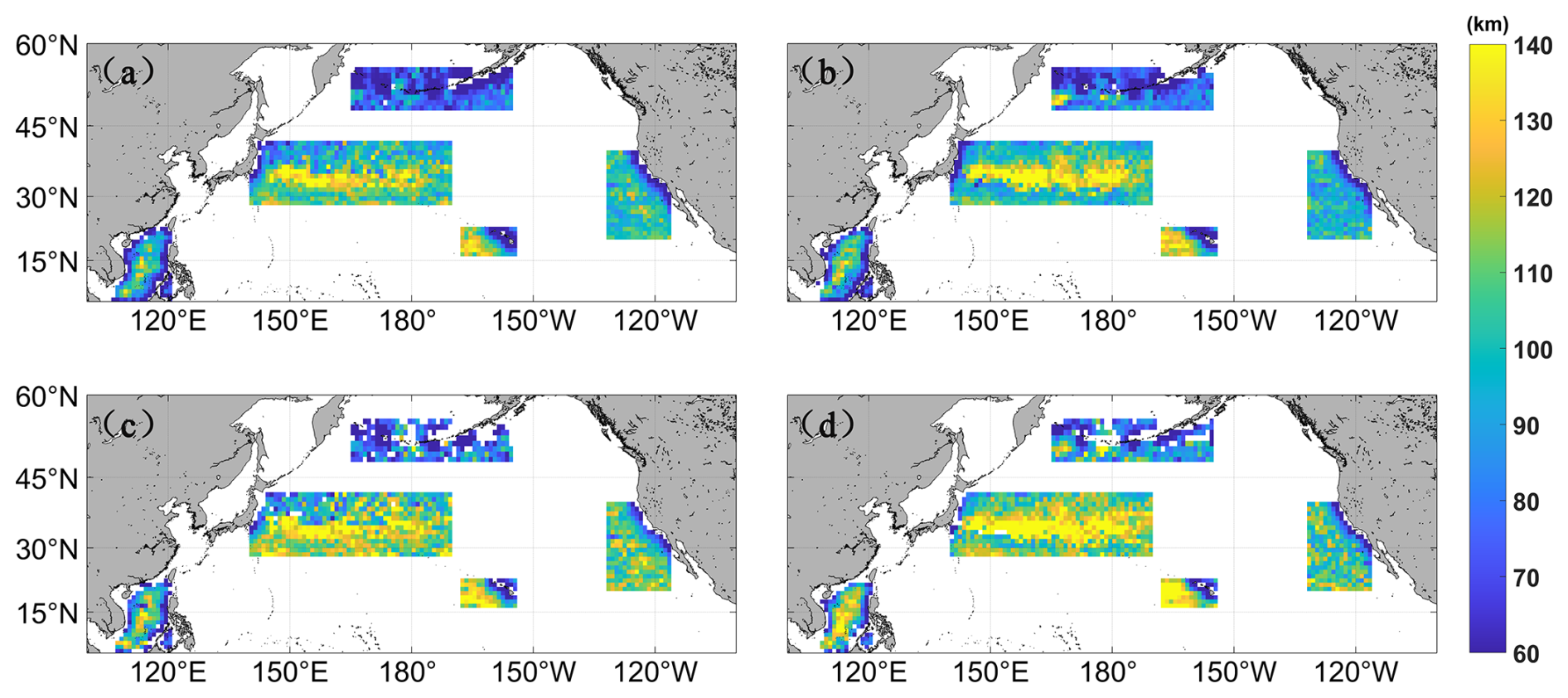
Figure 7 Spatial distributions of eddy radius for (a) CEs and (b) AEs identified under geostrophic balance conditions, and for (c) CEs and (d) AEs identified under cyclogeostrophic balance conditions.

We normalize the surface eddies that have a lifespan longer than 7 d. The X axis is divided by the lifespan of each individual eddy, while the Y axis variables are normalized by dividing each variable by its corresponding maximum value throughout the entire lifespan process.The average normalized eddy radius across the five regions exhibits a similar concave-up trend with the normalized eddy lifespan parameters and eddy kinetic energy (Fig. 8). The eddy radius of both CGEO and GEO shows a rapid increase during the formation phase, a slight growth slowdown during the development phase, stability during the mature phase, and a rapid decline during the dissipation phase.In the AI region (Fig. 8a), the normalized eddy radius curves of anticyclonic eddies are similar between the GEO and CGEO datasets during the eddy formation phase. For cyclonic eddies, however, the normalized radius of CGEO is significantly larger than that of GEO in the early formation stage. After correction of the CGEO data, the growth rate of CGEO eddies during the formation stage is lower than that of GEO eddies; during the mature phase, the normalized radius of CGEO eddies fluctuates more in both amplitude and frequency compared to GEO eddies. In the dissipation phase, the radius decay rate of GEO eddies is faster than that of CGEO eddies.In the KE region (Fig. 8b), the growth rate of CGEO eddies during the generation phase is lower than that of GEO eddies, while the radius decay rate of GEO eddies during the decay phase is higher than that of CGEO eddies. At both the initial generation and final decay stages, the radius of CGEO eddies is greater than that of GEO eddies; however, during the maturation phase, the maximum radius of CGEO eddies is smaller than that of GEO eddies.In the SCS region (Fig. 8c), the growth rate of CGEO eddies during the generation phase and the radius decay rate during the decay phase are both lower than those of GEO eddies. The radius of CGEO eddies is larger than that of GEO eddies at the initial generation and final decay stages. In the maturation phase, the peak radius of GEO-CE is slightly higher than that of CGEO-CE, while the peak radii of GEO-AE and CGEO-AE are similar.In the CC region (Fig. 8d), the growth rate of CGEO eddies during the generation phase and the radius decay rate during the decay phase are both lower than those of GEO eddies. At the initial generation stage, the radius of CGEO-AE is greater than that of GEO-AE, while the radii of CEs under the two balance conditions are similar. At the final decay stage, the radius of CGEO-CE is greater than that of GEO-CE, while the radii of AEs under the two balance conditions are similar. Additionally, during the generation phase, the growth rate of CGEO-CE radius is greater than that of GEO-CE, while the growth rates of CGEO-AE and GEO-AE are similar; the opposite trend is observed during the decay phase.n the HI region (Fig. 8e), the growth rate of CGEO eddies during the generation phase and the decay rate during the decay phase are both lower than those of GEO eddies. When eddies are initially generated, the radius of CGEO-CE is larger than that of GEO-CE, while the radii of AE under the two balance conditions are similar. At the final decay stage, the radius of CGEO eddies remains greater than that of GEO eddies.Overall, across the five regions, the radii of GEO eddies are comparable between the initial generation and final decay phases. For the modified CGEO dataset, the growth of AE during the generation phase is greater than that of CE, while the decay of AE during the decay phase is slower than that of CE. When CGEO eddies are initially generated, the radius of CE is larger than that of AE; however, by the final decay phase, the radius of CE becomes smaller than that of AE.Across the five regions, the growth rate of CGEO eddies during the generation phase is lower than that of GEO eddies, while during the decay phase, the radius decay rate of GEO eddies is faster than that of CGEO eddies. Additionally, AE in the modified CGEO dataset exhibits better radius retention characteristics.

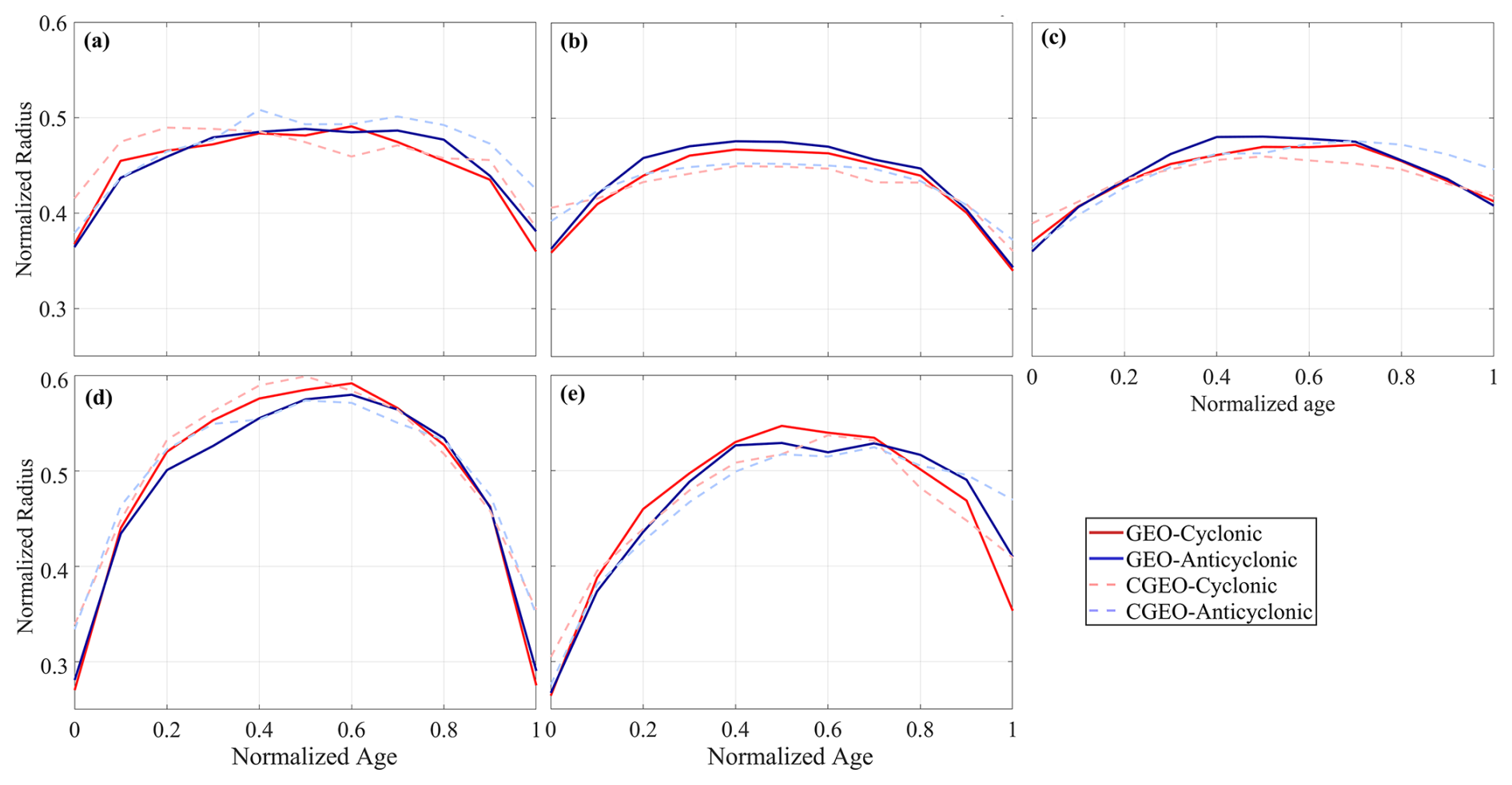
Figure 8 Temporal evolution of the mean normalized radius for the (a) SCS, (b) CC, (c) KE, (d) AI, and (e) HI. Each life stage is defined by normalized age: generation ($\sim \mathrm{0}-\mathrm{0.1}$), intensification ($\sim \mathrm{0.1}-\mathrm{0.3}$), maturation ($\sim \mathrm{0.3}-\mathrm{0.8}$), and decay (>0.8).

3.3 Eddy Generation and Dissipation

To examine the temporal patterns of eddy activity, formation and dissipation times were derived from the initial and final records of each tracked eddy. Across all five study regions (Fig. 9), the geostrophic framework consistently detects more eddy generation and dissipation events than the cyclogeostrophic framework, despite sharing similar interannual variability. The SCS (Fig. 9a and b) and CC (Fig. 9c and d) regions show significant reductions (averaging approximately 30 %–45 %), with the decrease for cyclonic eddies (CE) typically exceeding that for anticyclonic eddies (AE). In contrast, a greater number of eddies are identified in the KE region (Fig. 9e and f). However, it exhibits the smallest relative difference between the detection frameworks (averaging 20 %–33 %), a result that may be attributed to its strong background currents and eddy dynamics. The difference is most extreme in the AI region (Fig. 9g and h), where the average generation and dissipation counts under the CGEO framework are only about 40 %–50 % of those under the GEO framework (mean differences: AE about 60 %, CE about 50 %). This indicates that the cyclogeostrophic correction exerts a substantial impact on eddy detection outcomes in this high-latitude area. The case of the HI region is the most distinctive (Fig. 9i and j). It exhibits very high interannual variability and, in some years (e.g., 1994, 2002), shows negative differences (i.e., CGEO counts are higher than GEO counts). This can be attributed to the complex local dynamics in the HI region, which enhance the detectability of eddies after cyclogeostrophic correction.

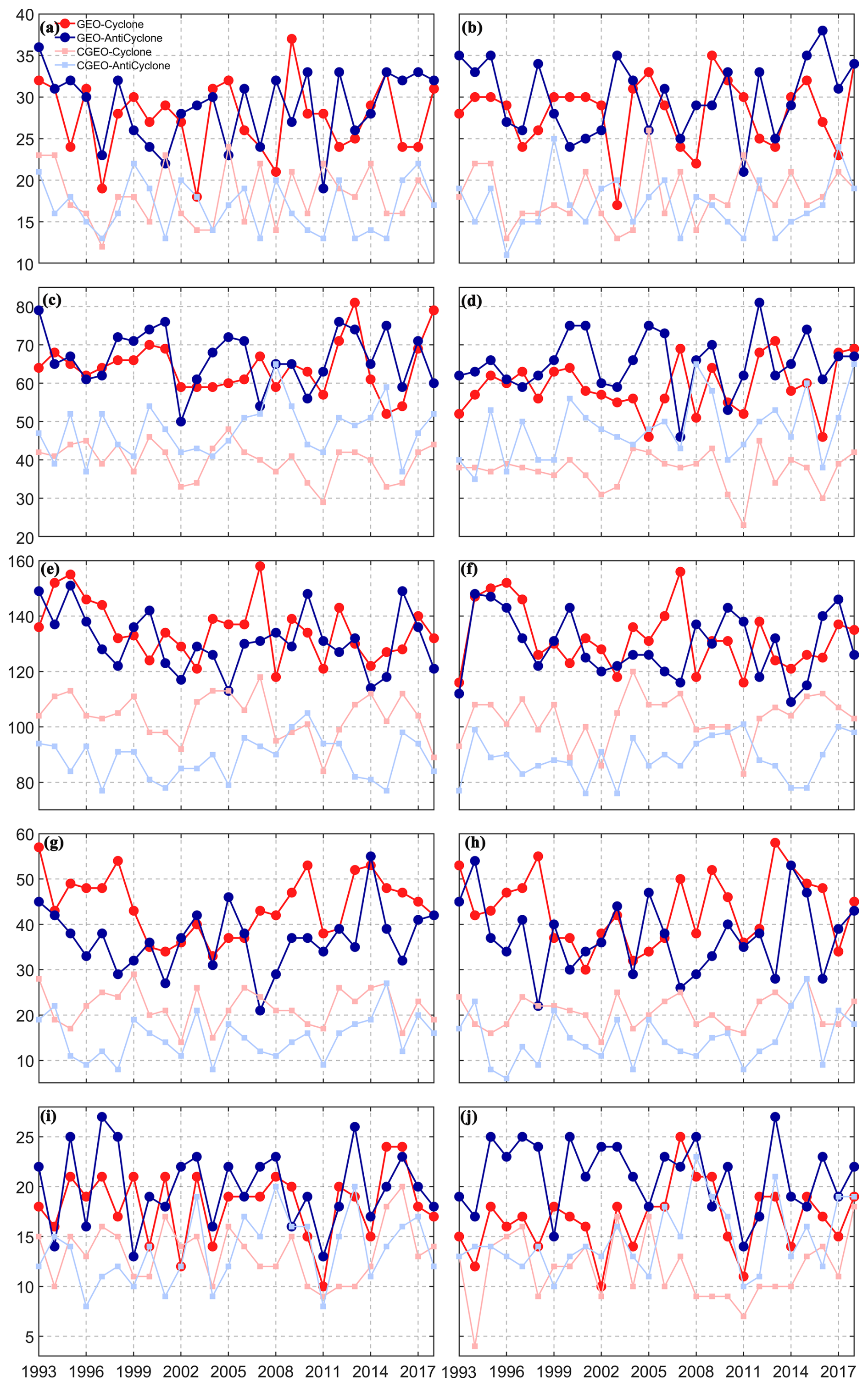
Figure 9 Interannual average time series of eddy generation and dissipation numbers (January 1993–December 2018). (a, b) SCS; (c, d) CC; (e, f) KE; (g, h) AI; (i, j) HI. The left column (a, c, e, g, i) shows eddy generation, and the right column (b, d, f, h, j) shows eddy dissipation. The dashed blue and red lines represent GEO-CE and GEO-AE, respectively. The dashed solid light blue and red lines represent CGEO-CE and CGEO-AE, respectively.

The spatial distributions of eddy generation and dissipation are presented in Figs. 10 and 11, respectively, with the analysis based on 1°×1° grids and including only eddies that persist for more than four weeks. Overall, the number of eddies generated and dissipated under cyclogeostrophic (CGEO) balance is lower than under geostrophic (GEO) balance; however, the spatial patterns of eddy distribution remain similar under both dynamical frameworks. In the AI region, GEO eddy abundance is higher in the northwestern and southeastern sectors, whereas CGEO eddies are more numerous in the eastern part of the region. Notably, the CE count surpasses that of AE in this region. In the KE region, the two datasets exhibit a notable consistency: fewer eddies are generated along the central axis of the Kuroshio Extension, while more AEs (to the north) and CEs (to the south) are produced. In the SCS region, eddy generation occurs more frequently in the eastern sector, including the Luzon Strait and west of the Philippines. In addition, markedly fewer CGEO eddies (Fig. 10c and d) are observed in the southern SCS compared to GEO eddies (Fig. 10a and b). In the CC region, eddy generation is predominantly concentrated in the eastern and southwestern coastal zones. In the HI region, eddies are clustered to the west of the Hawaiian Islands, and the number of CGEO-AEs (Fig. 10c) exceeds that of CGEO-CEs (Fig. 10d).

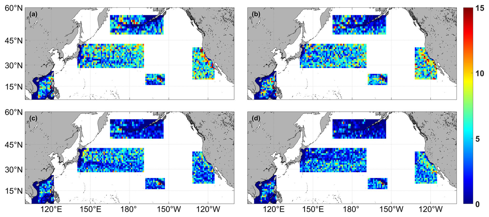
Figure 10 Spatial distribution of the number of eddies generated. The AEs and CEs detected by geostrophic currents are shown in (a, b), respectively. The AEs and CEs detected by cyclogeostrophic currents are shown in (c, d).

As shown in Fig. 11, in the KE region, cyclonic eddies (CEs) (Fig. 11b and d) are predominantly distributed south of the Kuroshio Extension axis, while anticyclonic eddies (AEs) (Fig. 11a and c) are concentrated to the north. In the CC region, eddy dissipation occurs mainly in the coastal areas, whereas in the HI region, it is distributed along the western coast of the Hawaiian Islands. In the AI region, the dissipation of GEO eddies is largely concentrated in the eastern and southwestern sectors, while that of CGEO eddies is focused primarily in the east. In the SCS region, the number of CGEO eddies generated in the southern part is notably lower than the number of GEO eddies in other areas of the basin.

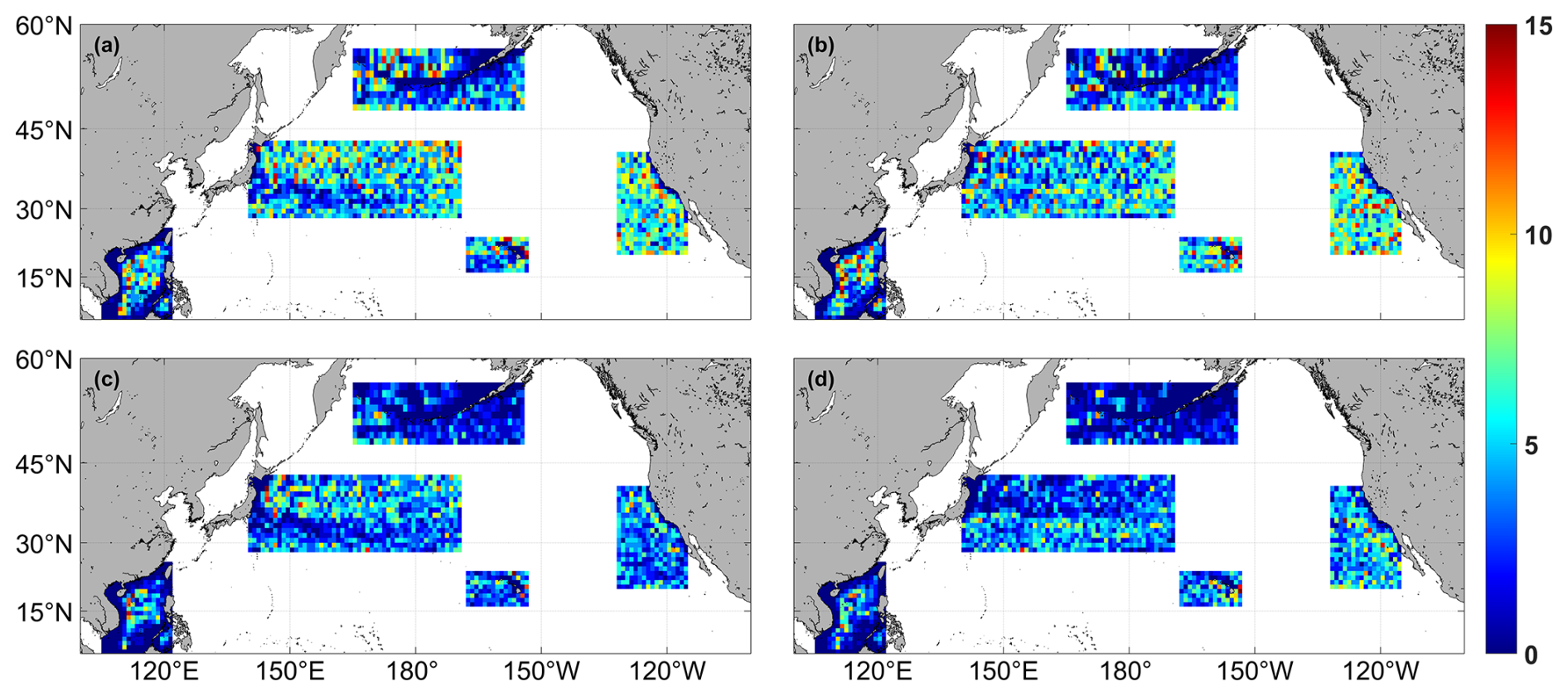
Figure 11 Same as Fig. 10, but for the number of eddy dissipations.

3.4 Movement and Propagation

As revealed by the statistical analysis of zonal velocity in Fig. 12, CEs and AEs generally exhibit similar translational speeds and directions in most regions, with the exception of certain areas within the SCS. The average difference in eddy translational speed is mostly below 0.5 cm s⁻¹, with CGEO eddies displaying greater speed variability than GEO eddies. Eddies in all five regions propagate westward. However, in all regions except HI, the westward speed decreases as latitude increases. Regional differences are also observed in the meridional movement: only in the CC region do both CEs and AEs move southward, with CEs propagating more slowly than AEs in that area. Further analysis of the relationship between westward speed and latitude indicates that in the AI and HI regions, the westward speed of CEs derived from CGEO data exceeds that from GEO data. Moreover, CGEO eddies exhibit more pronounced speed fluctuations than GEO eddies, generally following the pattern of increasing westward speed with decreasing latitude. The maximum westward speed occurs in the HI region around 20° N. A notable difference is that variations in westward speed have a stronger influence on CEs (Fig. 12a) than on AEs (Fig. 12c). Furthermore, for northward velocity (Fig. 12b and d), CGEO exhibits greater variability than GEO, with the SCS region showing the largest fluctuations overall. This can be attributed to a combination of high regional EKE, strong background flow interactions (Chen et al., 2011), and the low-latitude setting of the SCS, where the gradient wind balance dictates that centrifugal effects are amplified, significantly influencing eddy speeds (Shakespeare, 2016; Cao et al., 2023).

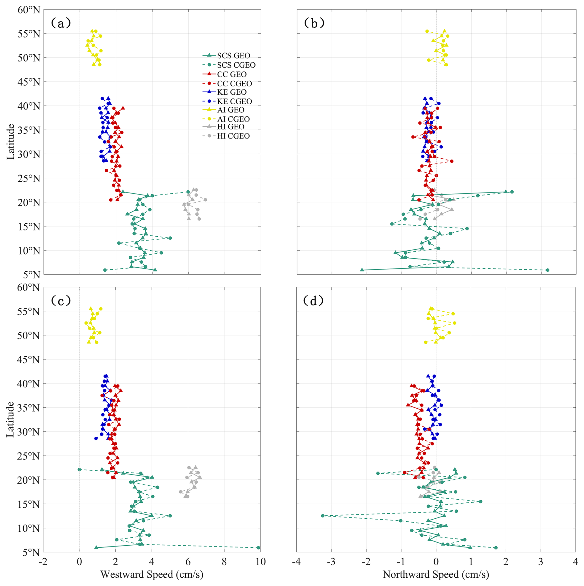
Figure 12 Latitudinal variations in the (a) zonal and (b) meridional speeds of CEs, and (c) zonal and (d) meridional speeds of AEs. Dashed and solid lines denote results from the CGEO and GEO balances, respectively.

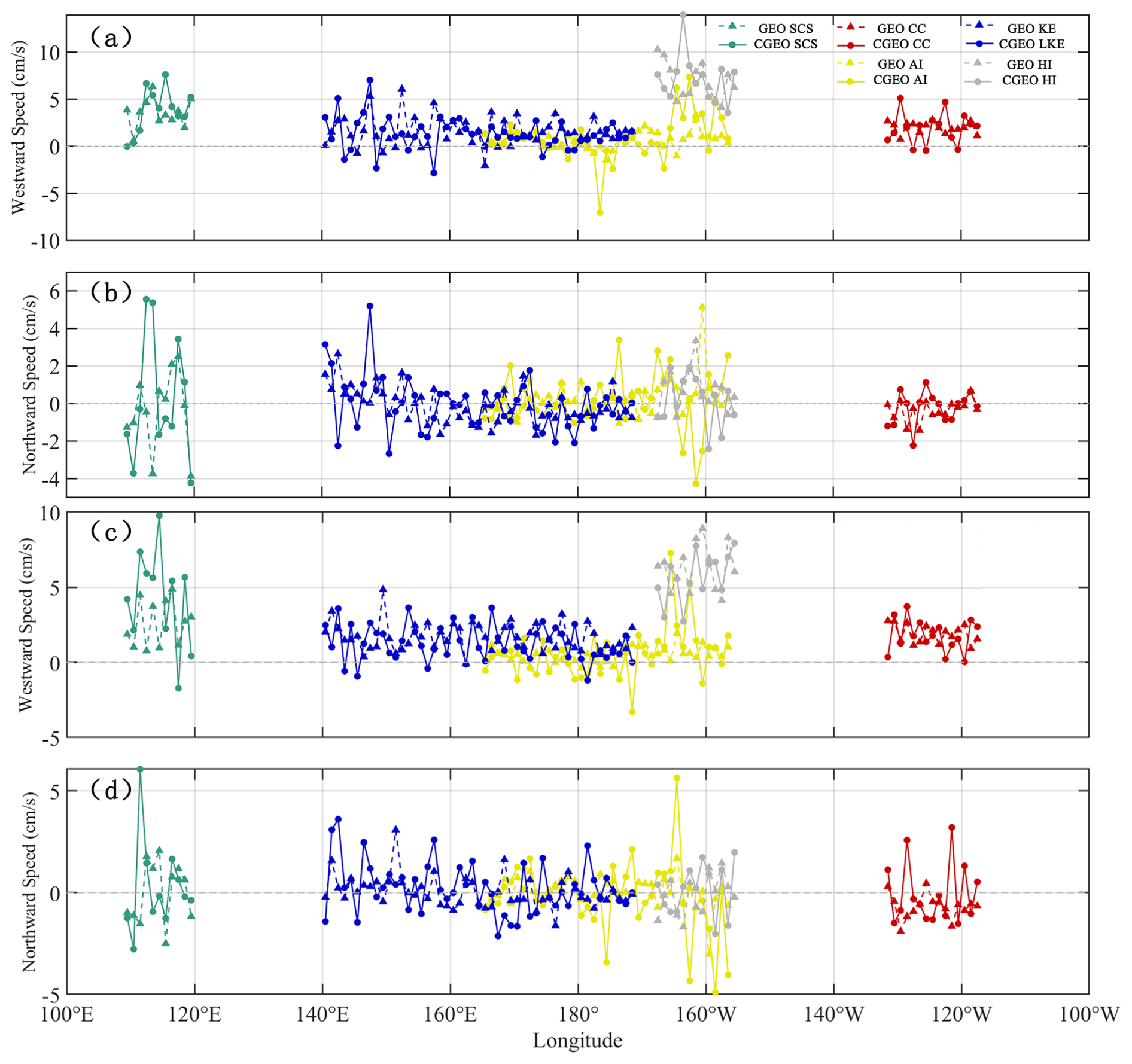
According to the meridional statistics, the speed variation of CGEO is more fluctuating than that of GEO (Fig. 13). Both CGEO and GEO eddies mainly move westward, with speeds ranging from 0–7 cm s⁻¹. In the HI region, the westward speed is faster, ranging from 4–14 cm s⁻¹, while AI, KE, and CC occasionally exhibit eastward fluctuations, with speeds under 3 cm s⁻¹. In the AI region, the CE (AE) moves eastward around 176° W (171° W) in CGEO data, with a speed of around 7 cm s⁻¹. The westward movement speed in the AI region around 165° W shows a large speed difference between the two datasets, with a difference greater than 5 cm s⁻¹. In the SCS, the speed difference between the two datasets is significant around 103° E, exceeding 7 cm s⁻¹. For CGEO-CE, the northward speed variation is large in the SCS region around 102° E, the western KE, and the eastern AI region, with northward and southward speeds reaching about 5 cm s⁻¹. In other regions, the speed fluctuations remain within the range of −2 to 2 cm s⁻¹. For CGEO-AE, the northward speed variation is also large in the SCS region around 102° E, the western KE, and the eastern AI region, but the maximum values in the SCS and AI regions are higher than those for CE, while the maximum value in KE is smaller than that for CE. The data correction has a greater impact on AE than on CE, with the speed difference in the northward movement for AE being noticeably larger than that for CE in both datasets.

Figure 13 Same as Fig. 12, but showing the variations by longitude.

3.5 Vorticity and Strain Rate

By definition, vorticity measures the local rotation rate of a fluid element. Given that rotation occurs about a specific axis, vorticity is therefore naturally represented as a vector. Theoretically, vorticity reaches its maximum at the eddy center and exhibits a radial decay, diminishing to zero at the eddy boundary. Therefore, the maximum vorticity value is adopted to represent the eddy's relative vorticity in subsequent analyses (Batchelor, 2000). The strain rate, in contrast, measures the eddy's capacity to deform and mix ambient fluid. It is a key parameter for understanding eddy-driven material transport, energy transfer, and the generation of secondary processes. In the SCS region, the normalized vorticity under GEO balance increases rapidly during eddy generation, significantly exceeding the CGEO values (Fig. 14a). For strain rate (Fig. 14b), CGEO maintains a higher overall magnitude than GEO, but exhibits a much lower rate of increase during the decay stage. In the CC region (Fig. 14c and d), the variation trends of GEO and CGEO are generally similar. Throughout the generation phase, the vorticity increase in GEO is relatively small. However, the normalized vorticity of GEO-AE rises more markedly than that of CGEO-AE, whereas the normalized vorticity of CGEO-CE begins to decay directly. Notably, CGEO-CE shows a slight increase during the dissipation phase. GEO and CGEO show comparable declining trends in strain rate, but the dissipative increase is markedly smaller for CGEO. The KE region (Fig. 14e and f) shows that CGEO vorticity decays slowly, yet remains higher than GEO during both the initial generation and final dissipation phases (Penven et al., 2014). The strain rate variations of GEO form a shallow concave shape, while those of CGEO remain stable initially before rising during dissipation. By comparison, the decline of CGEO is sharper and its recovery slower. As seen in the AI region (Fig. 14g and h), overall vorticity curves display more pronounced fluctuations. During generation, cyclonic eddy (CE) vorticity in both frameworks increases at comparable rates. For anticyclonic eddies (AE), GEO-AE shows a mild increase while CGEO-AE experiences a slight decrease, though GEO-AE retains a higher initial value. By the maturation phase, CGEO-AE undergoes noticeable growth that continues into dissipation, eventually resulting in a higher dissipation value than GEO-AE. Anticyclonic eddies also exhibit greater variability in strain rate compared to cyclonic eddies. Notably, CGEO strain rate falls faster but recovers more slowly than GEO. In the HI region (Fig. 14i and j), the vorticity increase of CGEO during generation is smaller than that of GEO, and its decay rate during dissipation is also lower. Although CGEO vorticity exceeds GEO at both initial and final stages, its peak value during maturation is lower (Shakespeare, 2016; Ioannou et al., 2019). The strain rate shows an approximately concave decline. The rates of decrease and increase during generation and dissipation are higher for GEO than for CGEO. Specifically, the strain rate of GEO-AE experiences an upward trend followed by a decline during the eddy maturation phase. As shown in the Fig. 14, vorticityand strain rate exhibit an inverse relationship for most of the time shown. In fluid dynamics, vorticity (describing local rotation) and strain rate (describing local stretching/shearing) collectively form the velocity gradient tensor, providing a complete kinematic description of a fluid parcel's motion (Kim, 2010). From an energy perspective, they jointly partition the kinetic energy of turbulence or disturbances. Under certain conditions, an increase in one quantity may occur at the expense of the other.

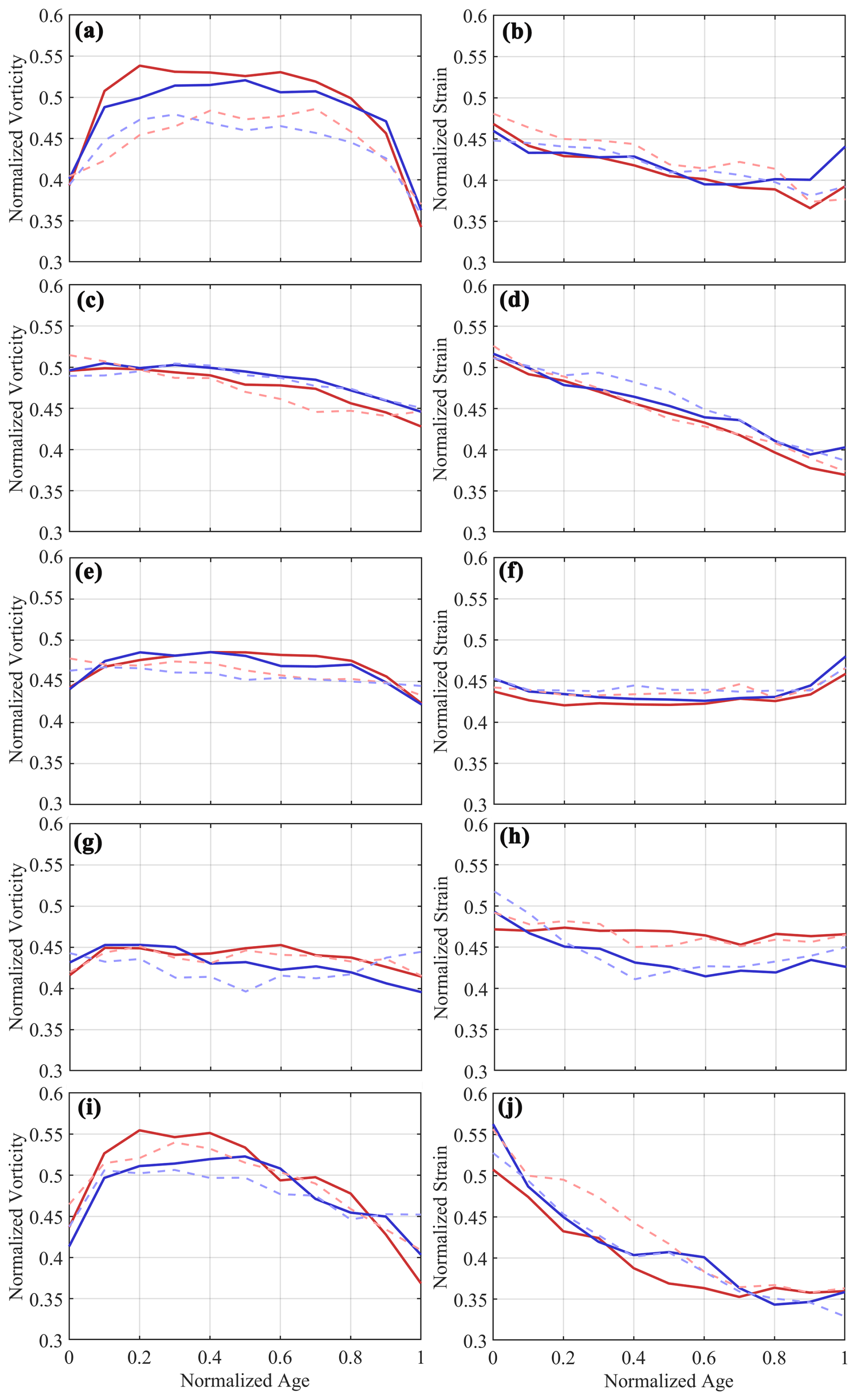
Figure 14 Time series of mean normalized relative vorticity (left) and strain rate (right) for five regions (1993–2018). Lines denote GEO (dashed) and CGEO (dash-dotted) frameworks for cyclonic (blue) and anticyclonic (red) eddies. (a, b) SCS; (c, d) CC; (e, f) KE; (g, h) AI; (i, j) HI.

3.6 Case Studies

Statistical analysis of eddies in five North Pacific regions exhibiting significant differences between cyclogeostrophic and geostrophic EKE differences shows that streamline curvature substantially influences both fundamental eddy characteristics (such as lifespan, radius, formation, and dissipation) and key eddy parameters, including intensity, strain rate, and effective EKE. This influence is particularly strong in high-energy and low-latitude areas. In order to further explore the impact of streamline curvature on the evolution process of eddies, a comprehensive analysis was conducted on selected individual cases of both cyclonic and anticyclonic eddies from the SCS, KE, and HI regions.

The South China Sea, located at the lowest latitude among the five study regions, has a relatively small Coriolis parameter of approximately $\mathrm{2.4}\times {\mathrm{10}}^{-\mathrm{5}}\mathrm{rad}{\mathrm{s}}^{-\mathrm{1}}$. To investigate the impact of cyclogeostrophic correction, a pair of dipole eddies in the SCS were analyzed for differences in its dynamics and evolution. The CE is characterized by maximum negative differences: −24.38 % (Fig. 15a) in velocity, −24.5 % (Fig. 15b) in enstrophy, and exceeding −50 % (Fig. 15c) in strain rate. The AE, meanwhile, displays maximum positive differences of 36.91 % (Fig. 15a) in velocity and 53.86 % (Fig. 15b) in enstrophy, with a CGEO strain rate more than 50 % greater than its GEO counterpart (Fig. 15c). This suggests that after correction, the AE is subject to increased deformation and enhanced dynamic intensity (Ioannou et al., 2019). Furthermore, Fig. 15e reveals that the decay rate of CGEO-EKE for the AE is substantially higher than that of its GEO counterpart, whereas the decay amplitudes of the CE under the two frameworks remain relatively similar (Fig. 15d). Both streamline curvature and the Rossby number act as key dynamical parameters that govern the stability of curved currents and jointly limit the intensity of anticyclonic eddies (Buckingham et al., 2021).

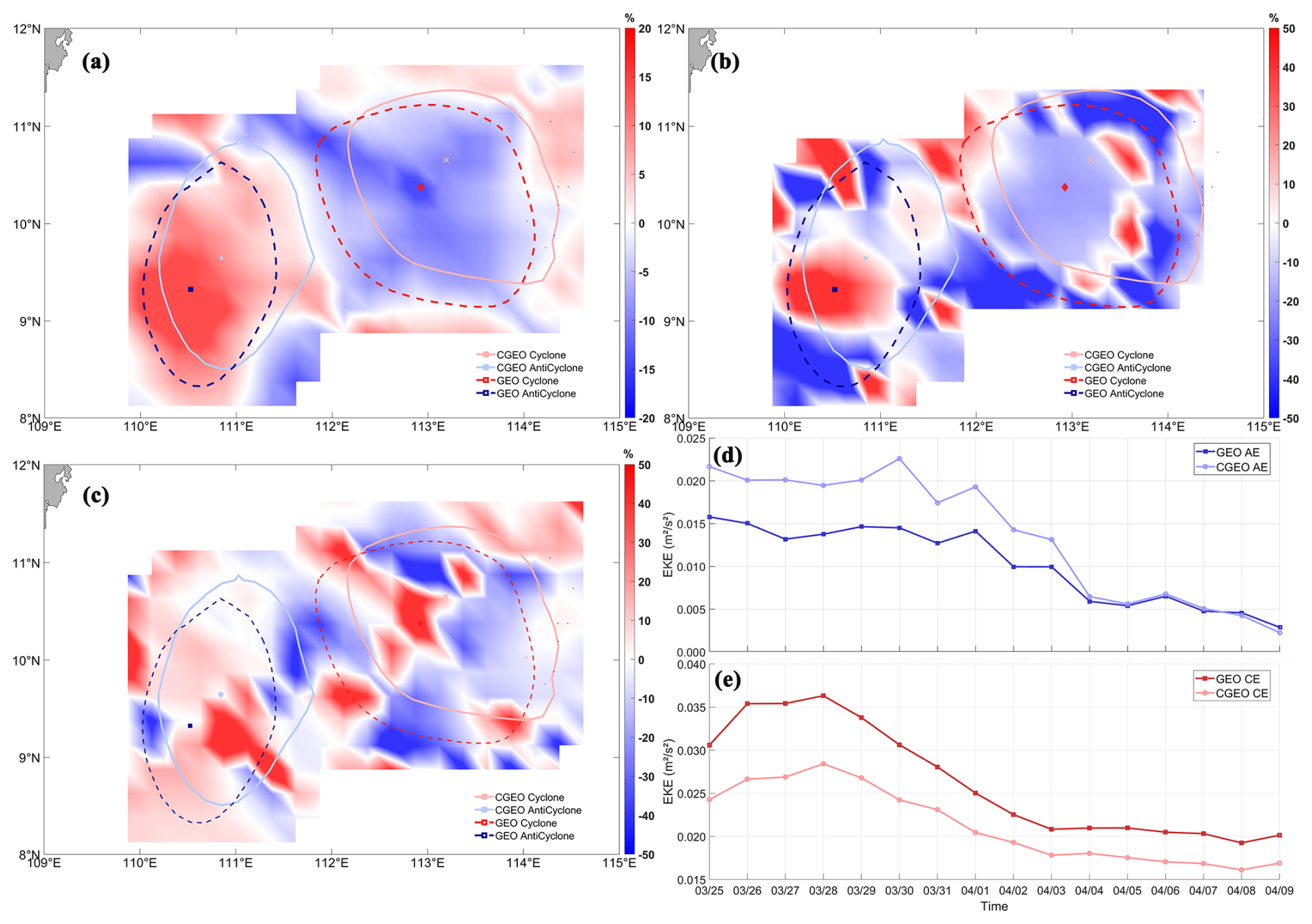
Figure 15 Snapshot of CE and AE cases in the SCS (25 March 2018): (a) Percentage difference between CGEO and GEO velocity; (b) Percentage difference between CGEO and GEO enstrophy; (c) Percentage difference between CGEO and GEO strain rate; (d) Evolution of EKE for a selected AE under CGEO and GEO balance (25 March–9 April 2018); (e) Evolution of EKE for a selected CE under CGEO and GEO balance (25 March–9 April 2018).

The Kuroshio Extension, as the western boundary current of the North Pacific subtropical gyre, is a highly unstable, strongly meandering and eddy-rich current. A cyclonic eddy (CE) and an anticyclonic eddy (AE) in this region were selected for case analysis. The CE is located between 33–34° N, with a Coriolis parameter of about $\mathrm{8}\times {\mathrm{10}}^{-\mathrm{5}}\mathrm{rad}{\mathrm{s}}^{-\mathrm{1}}$. After cyclogeostrophic correction, its maximum velocity decreased by approximately 20.67 % (Fig. 16a), the maximum eddy enstrophy dropped by about 31.36 % (Fig. 16b), and the strain rate was reduced by more than 50 % (Fig. 16c), while the Rossby number decreased from 0.133–0.105. In contrast, the AE is centered between 36–37° N, with a Coriolis parameter of approximately $\mathrm{8.7}\times {\mathrm{10}}^{-\mathrm{5}}\mathrm{rad}{\mathrm{s}}^{-\mathrm{1}}$. For the AE, the maximum velocity increased by about 23.57 % (Fig. 16a), the maximum eddy enstrophy rose by roughly 20.42 % (Fig. 16b), and the strain rate increased by more than 50 % (Fig. 16c). Chen and Han (2019) revealed a positive correlation between the kinetic energy of mesoscale eddies and their lifespan. They noted that variations in eddy kinetic energy reflect the length of the eddy life cycle. A comparison of the EKE evolution of the CE (Fig. 16d) and AE (Fig. 16e) under CGEO and GEO balance conditions shows that GEO balance overestimates the EKE of the CE while underestimating that of the AE. Compared to GEO balance, the CGEO-EKE of the AE decays more rapidly, whereas the decay amplitudes of the CE are similar under the two balance conditions.

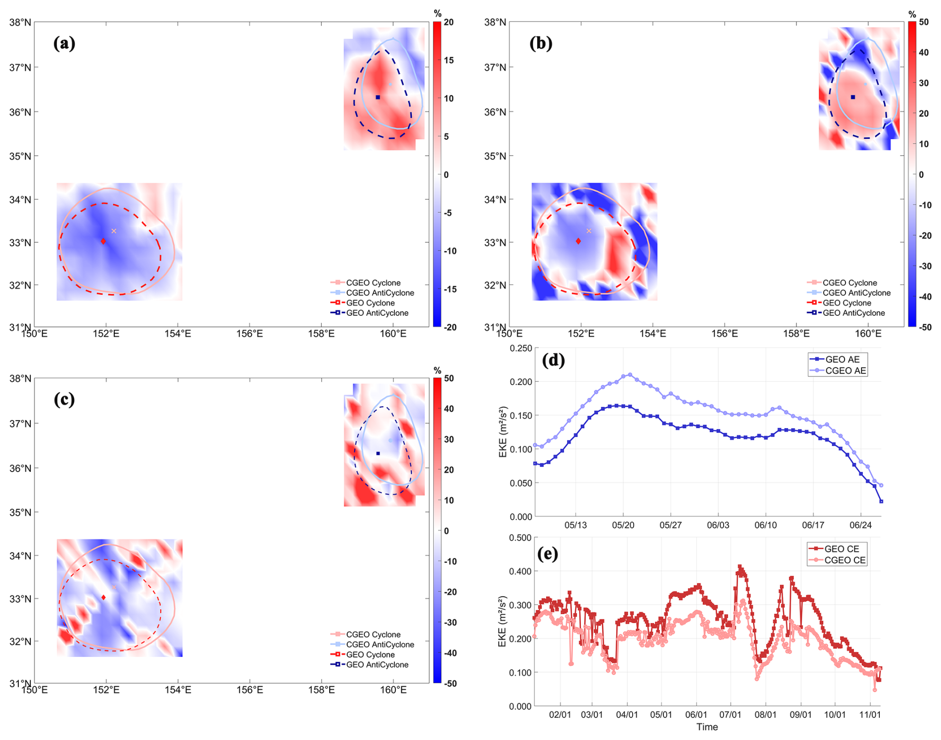
Figure 16 Snapshot of CE and AE cases in the KE region (25 May 2018): (a) Percentage difference between CGEO and GEO velocity, (b) Percentage difference between CGEO and GEO enstrophy, (c) Percentage difference between CGEO and GEO strain rate; (d) Evolution of EKE for a selected AE under CGEO and GEO balance (7 May–15 June 2018), (e) Evolution of EKE for a selected CE under CGEO and GEO balance (1 January–10 Novenmber 2018).

The HI region is a low-latitude oceanic area, with the selected eddies located between 18–19° N, where the Coriolis parameter is approximately $\mathrm{4.6}\times {\mathrm{10}}^{-\mathrm{5}}\mathrm{rad}{\mathrm{s}}^{-\mathrm{1}}$. For the CE, the Rossby numbers under GEO and CGEO balance are 0.118 and 0.114, respectively. Within the CE, the maximum velocity difference percentage (Fig. 17a) reaches 8.64 %, the maximum eddy enstrophy difference percentage (Fig. 17b) can reach −25.74 %, and the maximum strain rate difference percentage (Fig. 17c) is more than −50 %. For the AE the Rossby numbers under GEO and CGEO balance are 0.123 and 0.106, respectively. Within the AE, the maximum velocity difference percentage (Fig. 17a) reaches 26.42 %, the maximum eddy enstrophy difference percentage (Fig. 17b) is 43.37 %, and the maximum strain rate difference percentage (Fig. 17c) is greater than 50 %. This sensitivity of the cyclogeostrophic correction to the energy state of AEs highlights its fundamental importance in regulating their dynamical properties. A comparison of the CGEO and GEO evolution processes between the AE (Fig. 17d) and the CE (Fig. 17e) reveals distinct behavioral contrasts. In the AE, both the growth and decay rates of CGEO-EKE are higher than those under the GEO framework, and its peak EKE value also surpasses the GEO estimate. Conversely, the CE exhibits the opposite pattern, in which GEO-EKE shows higher growth and decay rates along with a larger peak value than its CGEO counterpart.

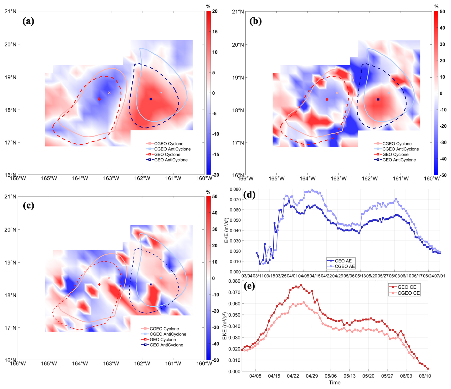
Figure 17 Snapshot of CE and AE cases in the HI region (25 May 2018): (a) Percentage difference between CGEO and GEO velocity, (b) Percentage difference between CGEO and GEO enstrophy, (c) Percentage difference between CGEO and GEO strain rate; (d) Evolution of EKE for a selected AE under CGEO and GEO balance (10 May–1 July 2018), (e) Evolution of EKE for a selected CE under CGEO and GEO balance (4 April–1 June 2018).

While Stegner and Dritschel (2000) noted that centrifugal force in shallow-water models stabilizes anticyclones but destabilizes cyclones, Shakespeare (2016) demonstrated that anticyclones sharpen more rapidly than cyclones under identical background strain. In a complementary finding, Buckingham et al. (2021) diagnostically showed that streamline curvature and the Rossby number together limit anticyclonic vortex intensity. Consequently, for altimeter-derived surface eddies, the action of centrifugal force leads to more pronounced differences in anticyclonic structures.

4 Conclusion

Mesoscale eddies are a key component of oceanic currents and a central focus in the study of ocean dynamic processes. The classical geostrophic balance neglects the nonlinear term arising from streamline curvature, which can introduce biases in sea surface velocities derived from altimeter data in curved currents. This is particularly relevant as Chelton et al. (2011) established that nearly all observed mesoscale features outside the 20° S–20° N tropical belt are nonlinear. Consequently, to quantify these biases, a statistical comparison of eddy characteristics across five North Pacific regions is conducted using both altimetry-based surface current velocities and their iteratively corrected cyclogeostrophic counterparts. This research compares the characteristics of cyclonic (CE) and anticyclonic (AE) eddies under geostrophic and cyclogeostrophic balances to evaluate how centrifugal forces modify eddy dynamics, with a focus on the systematic influence of correction on eddy energy, structure, and evolution.

A comparative analysis of the spatial distribution of EKE difference percentages and interannual evolution characteristics under the two balance conditions reveals that the difference patterns for eddies with negative and positive relative vorticity are completely opposite: after cyclogeostrophic correction, the EKE of CEs weakens, while that of AEs strengthens (Penven et al., 2014; Cao et al., 2023). On the temporal scale, cyclogeostrophic correction is more significant for the geostrophic flow field of AEs. Using the SCS as an example, the evolution of normalized EKE with the normalized eddy lifetime parameter shows that CGEO EKE increases faster during the growth stage, decays more slowly during the decay stage, and has higher energy retention (Ioannou et al., 2019). Meanwhile, the variation range of CGEO EKE is significantly smaller than that of GEO, confirming the regulatory role of cyclogeostrophic correction in balancing eddy energy distribution. From the perspective of lifecycle stages, the differences in energy evolution are distinct: during the generation and decay stages, the energy increase and decrease rates of CGEO eddies are generally lower than those of GEO estimates; in the mature stage, the two tend to converge. For AEs, cyclogeostrophic correction significantly accelerates energy decay, and the streamline curvature effect intensifies their instability, thereby promoting the dissipation process (Lazar et al., 2013).

Comparative analysis of eddy statistics shows a 35.65 % higher eddy census in the GEO framework compared to CGEO, despite strong agreement in their spatial distributions. The CGEO framework yields eddies with a larger mean radius but shorter lifetimes. We also find that cyclonic eddies (CEs) typically have longer lifetimes than anticyclonic eddies (AEs). This divergence in eddy longevity and scale suggests that streamline curvature effects promote deformation and energy dissipation, disproportionately affecting AEs. This aligns with the conclusion of Chen et al. (2019) that shorter eddy lifespans are associated with greater instability. The spatial distribution patterns of eddy radius are highly similar between the two datasets. The evolution of radius normalized by eddy lifetime follows the same trend as EKE evolution, showing an upward convex curve. During the generation phase, CGEO eddy radius increases more slowly than GEO eddy radius. During the decay phase, GEO eddy radius decays faster than CGEO eddy radius. In addition, GEO identify more eddies than CGEO during both generation and dissipation phases, but their interannual variations and spatial distribution characteristics are similar. In most regions, eddy westward propagation speed decreases with increasing latitude. The speed variation curve of CGEO eddies fluctuates more significantly than that of GEO eddies. Cyclogeostrophic correction generally has a stronger effect on CEs than on AEs. Differences in eddy enstrophy and strain rate further confirm that anticyclonic eddies are more sensitive to curvature, with enhanced dynamical characteristics after correction (Shakespeare, 2016).

An analysis of regional eddy case differences reveals the latitudinal dependence of streamline curvature effects: cyclogeostrophic correction has a particularly significant impact in low-latitude regions (such as the SCS and HI) and strong current regions (such as the KE). This indicates that regions with small Coriolis parameters and high Rossby numbers are affected more strongly by streamline curvature effects (Cao et al., 2023). From the perspective of eddy types, cyclogeostrophic correction plays a more critical role in shaping the dynamical properties of AEs. However, for CEs, the streamline curvature effect slows their propagation, which weakens eddy kinetic energy, enstrophy, and strain, thus rendering them more stable (Shakespeare et al., 2016).

This study provides a systematic comparison of sea surface eddy characteristics under two dynamical frameworks. First, it reveals the operational constraints of the geostrophic approximation in strongly curved flows, suggesting that adopting the cyclogeostrophic balance in high Rossby number regions (e.g., low latitudes, western boundary currents) can yield more accurate kinetic energy estimates and eddy censuses. Second, the relative stabilization of cyclonic eddy evolution compared to anticyclonic eddies following cyclogeostrophic correction indicates a significant influence of centrifugal force on eddy instability mechanisms, a theory corroborated by Buckingham et al. (2021). In summary, this work offers methodological implications for future altimetry-based studies: to better quantify eddy-mediated energy transfer, particularly in dynamic oceanic hotspots, explicit inclusion of centrifugal forces is needed to mitigate systematic biases. Ultimately, integrating cyclogeostrophic dynamics can refine the framework for observing and interpreting the energetic complexity of mesoscale ocean turbulence.