Evaluation of Extreme Sea-Levels and Flood Return Period using Tidal Day Maxima at Coastal Locations in the United Kingdom

Tidal storm surges can result in significant inundation and damage if sea defences are insufficiently robust. Coastal planners need to know the risk of flooding so that sea defences and coastal developments can be specified and located appropriately. Since the original work on extreme value statistics by Gumbel (1954), several alternatives have been proposed for evaluating the risk of tidal inundation, with the Skew Surge Joint Probability Method (SSJPM) gaining popularity. However, SSJPM is complex and cannot always be applied generally. Guided by the search for a general method having wide application and amenable to automation, this paper re-examines the original approach of Gumbel and proposes a simple modification for combined peak selection and declustering; it is termed here TMAX, since it selects one maximum per tidal day. In comparison with the method of Gumbel (1954) using annual maxima (later termed AMAX), the TMAX method offers more efficient use of extreme data events and in addition, simpler handling of missing data. The results of the TMAX method are compared with those of a recent UK study using the SSJPM method at the same United Kingdom coastal locations. The broadly applicable TMAX method has the potential to offer more widespread calculation of flood return period, thereby improving strategies regarding coastal management and resilience.

1 Introduction

Coastal planners and developers require estimates of coastal flood risk for planning, design and siting of sea defences, coastal buildings, harbours, nuclear power stations, and other critical infrastructure. Estimating flood risk is especially challenging for low-lying coastal areas, including parts of the United Kingdom (UK), (Williams et al., 2016). Coastal floods generally occur when a significant storm surge occurs at or near the time of a spring high tide.

The required height of sea defences can vary quite rapidly along the coastline. This is because the coastal seabed topography can locally magnify or diminish the effects of tidal and surge effects. Tide gauge data provides a statistical snapshot relevant to its location; whether it is sited in an exposed coastal location or in a sheltered harbour, the recorded information can serve as a vital local source for estimating flood probability and return period. Tide gauge data is traditionally used for the establishment of tidal levels such as the Highest Astronomical Tide (HAT), see Doodson and Warburg (1941) and for tidal harmonic analysis where it finds use in tidal prediction and in the determination of boundary conditions for tidal modelling and in their numerical validation (Zhang et al., 2003). However, extreme sea-level analysis can leverage the same tide-gauge data to predict the flood return probability. It is important here to distinguish between HAT and extreme flood height. HAT assumes average conditions for the meteorological component, whereas the conditions leading to extreme flooding include the effects of the meteorological component. Throughout this paper, the term tide refers to the total fluctuating sea level, while the astronomical tide refers to the deterministic predicted component caused by tidal forces generated by the earth-solar and lunar-earth orbits. The difference between the two is termed the residual. The residual, especially when large, may be caused by a storm surge but this is not necessarily the case. Similarly, although the residual may often result from meteorological effects and may appear as noise it may contain a deterministic component, and the terms noise and storm surge are generally best avoided in this context. The term “ESLs” is used, throughout this paper and within the relevant literature to mean “estimates of the exceedance probabilities of Extreme Sea-Levels” (Batstone et al., 2013). Several statistical methods have been developed to assess Extreme Sea Levels (ESL) from sea level measurements, these are now briefly reviewed.

The original work by Gumbel (1954) describes a method for the conversion of maxima into ESLs, with the majority of cases being based upon the analysis of annual maxima; this later became known as the AMAX method. Since AMAX uses annual maxima, significant events that rank second or lower each year are not utilised. However, in his original work, Gumbel also examined some extreme events without using annualized data, such as the breaking point of yarn and the breakdown voltage of electrical capacitors. Subsequently an approach based upon threshold rather than grouping has become known as the “Peaks over Threshold” (POT) method, see Coles (2001), while an approach based upon selection of the largest, r, peaks within each time block has become known as the “r-largest” method (Smith, 1986; Tawn, 1988).

A different approach by Pugh and Vassie (1978) splits the total sea level into two components which sum to the total tide: these are the deterministic astronomical tide component and the residual component. Each component is converted into separate probability distributions which are then combined by convolution to produce a joint probability distribution function (PDF). The method is known as the joint probability method (JPM). Its main advantage lies in its efficient use of source data; all values of the residual contribute to the final probability distribution function (PDF), even if they are not at or near high tide. However, there are two notable drawbacks to the JPM. First, the conversion of the PDF into design risk is challenging, as it can depend on sampling period (Middleton and Thompson, 1986; Tawn et al., 1989). Second, in practice the timing of actual high tide is often shifted in relation to the underlying predicted astronomical tide; this introduces correlation between two components, undermining the convolution (Tawn, 1992). Nevertheless, the JPM is widely used (Pirazzoli and Tomasin, 2007; McInnes et al., 2013), despite these known deficiencies (Batstone et al., 2013).

The skew surge joint probability method, SSJPM, aims to overcome the shortcomings of the JPM, by replacing the residual (i.e. the instantaneous difference of measured and predicted water level) in JPM with the height difference between the maxima of the measured and predicted water level for each tidal cycle. This new height difference, referred to as the “skew surge height”, is claimed to have minimal correlation with tidal height at most locations and is therefore considered an ideal parameter for characterizing surge statistics (Williams et al., 2016). To accurately extrapolate the tail of the probability curve, an extreme value probability distribution, such as the generalized Pareto distribution (GPD), is used. The SSJPM method was used in the UK Environment Agency Study (2011); as described by Batstone et al. (2013), (referred to from here onwards as EA2011) which was based upon source data from the UK National Tide Gauge Network (UKNTGN). However, Batstone et al. (2013) reported: ”The ESL's values derived from the SSJPM were compared with the AMAX time series of sea-level.”, ”At approximately one-quarter of the UKNTGN sites, it became clear that the GPD fitted on the skew surge distribution was leading to a seemingly implausible representation of the most extreme sea levels.”..”Adjustments to the GPD shape parameter were performed by averaging the value with four immediate neighbours weighted by the length of data at each site”. The problem was attributed to correlation between skew surge and predicted tide. Williams et al. (2016), reported that when “seasonal relationships between tides and the storm season were removed, then skew surge and associated HW are completely independent at 68 of our 77 study sites”. Thus, even after removing seasonal effects, skew surge and associated HW were not completely independent at a minority, but significant number, of locations. Here is the dilemma of the SSJPM method. It works well when the skew surge is independent of the tide but how can we know in advance when this is the case? As we have seen, in EA2011, approximately one-quarter of the locations in that study had to be re-examined and re-calculated using other adjustments. Since EA2011 a further modification known as the quasi-nonstationary skew surge joint-probability method (qn-SSJPM) method has evolved which treats long term tidal constituents separately. See Baranes et al. (2020); Enríquez et al. (2022).

The above situation indicates that it may be useful to return to a simple, generally applicable method of estimating ESL's, rather than using extended methods which are intended to be maximally accurate but are manually intensive. Such a tool may facilitate broad regional and global studies of coastal flood hazard risk (e.g. Hunter et al., 2017; Martín et al., 2024; Zhang and Convertino, 2026). This paper pursues such a goal by re-examining the method of Gumbel (1954) and incorporating a relatively simple modification within it. The results of this approach, called here TMAX, are compared with the EA2011 study which used the SSJPM method. Unlike in EA2011, the TMAX method did not require manual intervention, and used an identical algorithm for each location. The primary purpose of this study is to examine the suitability of the TMAX technique, by comparing its results with those of the AMAX and SSJPM methods using the results of EA2011. Although it would be useful to extend this comparison beyond the UK, at the time of writing this study was constrained by the availability of data and is therefore limited to a comparison to data from a previous study at 41 UK locations as described in Batstone et al. (2013), and in EA2011. Across these UK locations, the tidal ranges are largest in the South West, with spring tides being over 12 m in the Severn Estuary. The UK region also suffers generally from weather induced tidal surges, with over 2 m excess surge having been recorded in the North Sea in 1953 and 2013. The purpose of this study is to examine the proof of concept for the described TMAX method, rather than being an attempt to redefine UK ESL flood defence heights.

2 Background

Fuller (1914) claimed that, on a purely empirical basis, the size of floods increases proportionately to the logarithm of observation time. Some 40 years later Gumbel, in his seminal 1954 paper “Statistical Theory of Extreme Values and Some Practical Applications”, theoretically justified Fuller's claim, provided the extreme values are derived from a stationary series, i.e. one whose mean did not drift uniformly with time, and have a probability distribution of an exponential type. This latter condition, later known as a Gumbel/Fisher-Tippett Type I distribution, applies but is not limited to exponential, normal, chi-squared, logistical and log-normal distributions (See also Leadbetter, 1983; Tawn, 1988). Gumbel gave many practical examples ranging from floods, radioactive decay, human life expectation, electrical capacitor breakdown, the strength of yarn, and the stock market share value. In Gumbel's original description (see his Eq. (2.17)), a number, N, of observed peak values (generally annual), were ranked in ascending order with each ranked value i, being converted into the cumulative probability of a value not exceeding the ranked value, F_i by the formula

$$\begin{array}{}\text{(1)}& F_i=i/(N+\mathrm{1})\end{array}$$

The probability F_i is related to the return period T (generally in years) by Gumbel's Eq. (2.8), i.e.

$$\begin{array}{}\text{(2)}& T_i=\mathrm{1}/(\mathrm{1}-F_i)\end{array}$$

Gumbel showed that for a Type I distribution, the probability of the value being below a given value can be written as

$$\begin{array}{}\text{(3)}& F=\exp (-\exp \left(-y\right))\end{array}$$

The reduced variate, y exhibits a linear relationship with observed extreme value x, via a scale factor α and location factor, μ being given by

$$\begin{array}{}\text{(4)}& y=\mathit{\alpha }(x-\mathit{\mu })\end{array}$$

Therefore, in a plot of observed extreme height x, versus reduced variate y, each extreme value falls approximately in a straight line. In Gumbel's time, each ranked value was physically plotted on probability paper, where the horizontal scale had been marked out according to Eq. (3), in terms of either return period or reduced variate or both, depending upon the manufacturer of the paper. A straight line was fitted to the points, and extrapolation of the line gave the probability of a value not exceeding a given value x, without explicitly requiring the calculation of the scale factor, α or location factor, μ.

Returning now to Eq. (1), Gringorten (1963) proposed a widely accepted correction to improve the plotting accuracy as

$$\begin{array}{}\text{(5)}& F_i=(i-\mathrm{0.44})/(N+\mathrm{0.12})\end{array}$$

3 TMAX Method

The method described in this study named TMAX, differs from the method described by Gumbel in three main ways. Firstly, the ascending order of maxima used by Gumbel is replaced by a descending rank of maxima. Secondly, only one maximum is detected within each tide. Finally, only a subset of the total number of peak values are selected and used to fit the straight line in the probability plot. These differences are now considered in more detail.

3.1 Descending Rank

There are advantages in reversing the rank order as compared with Gumbel's original scheme, see Harris (1996), and this reversal is used here. Since the largest most extreme value is known it can readily be indexed as 1 while successively smaller values are indexed with rising integers (2, 3, etc). We consider here F(x) to be the probability of the tide exceeding a height value x (i.e. to be the flood probability), rather than the opposite as in Gumbel's original formulation. Adding a prime to those equations of Gumbel i.e. F in Eqs. (2) and (3) and noting that $F^{\prime }=\mathrm{1}-F$, Eqs. (2) and (3) now become

$$\begin{array}{}\text{(6)}& {\displaystyle }T=\mathrm{1}/(\mathrm{1}-F{}^{\prime })=\mathrm{1}/F\text{(7)}& {\displaystyle }T=\mathrm{1}-\exp (-\exp \left(-y\right))\end{array}$$

where y is the reduced variate. Making y the subject of Eq. (7) gives

$$\begin{array}{}\text{(8)}& y=-{\log }_e(-{\log }_e\left(\mathrm{1}-F\right))\end{array}$$

We note that F is very much less than 1, hence the right-hand logarithm can be represented by −F, and since F and T are inversely related we obtain y=log (T), confirming Fuller's original claim that maximum flood height varies with the logarithm of time. Writing Gumbel's descending rank, as i^′, the ascending rank, i, is given by $i=N+\mathrm{1}-i^{\prime }$ and substituting this into Eq. (1) we obtain

$$\begin{array}{}\text{(9)}& F_i=\mathrm{1}-Fi{}^{\prime }=\mathrm{1}-i^{\prime }/(N+\mathrm{1})=i/(N+\mathrm{1})\end{array}$$

and applying Gringorten's correction we obtain

$$\begin{array}{}\text{(10)}& \begin{array}{rl}{F}_i& =\mathrm{1}-Fi{}^{\prime }=\mathrm{1}-\left(i{}^{\prime }-\mathrm{0.44}\right)/\left(N+\mathrm{0.12}\right)\\ & =(i-\mathrm{0.44})/(N+\mathrm{0.12})\end{array}\end{array}$$

Since Eq. (10) is identical in form to Eq. (5) the reversal of rank order does not affect Gumbel's original plotting formulae, nor Gringorten's correction to it. The Gringorten formula, rather than Eq. (1), was used in all of the relevant calculations from hereon. The design risk D(x), i.e. the probability that a given value of x will be exceeded during a design life consisting of n durations (usually years), is given by.

$$\begin{array}{}\text{(11)}& D\left(x\right)=\mathrm{1}-(\mathrm{1}-F\left(x\right){)}^n\end{array}$$

3.2 Tide Peak Detection Algorithm

Most but not all of the examples given by Gumbel use the annual maxima. However, Gumbel stated in his conclusion, “If the number of observed extremes N is not excessive, do not group the observations”. Therefore, although extrema are generally grouped into annual time blocks, it is not necessary to do so. In the TMAX method described here, maxima are not explicitly grouped. The largest peaks in the tide gauge record are identified as follows. The data is initially scanned and the mean sea-level height value, m.s.l., is found. The data is again re-scanned, and when the height value transitions above m.s.l. a search flag is set and the date and time of the upwards transition is stored. Once the search flag is set, the highest value is determined until the sequence transitions downwards below the m.s.l. At this point the search flag is unset and the date and height of the highest value found during the period when the tide is above m.s.l. Provided that the date-time of the downwards transition minus the date-time of the upwards transition is less than a tidal day the event is stored in a list as a maximum. This latter condition avoids counting transitions when the data has large gaps. Furthermore, this strategy also prevents the selection of multiple peaks from within the same storm event, thereby providing a degree of declustering (see below).

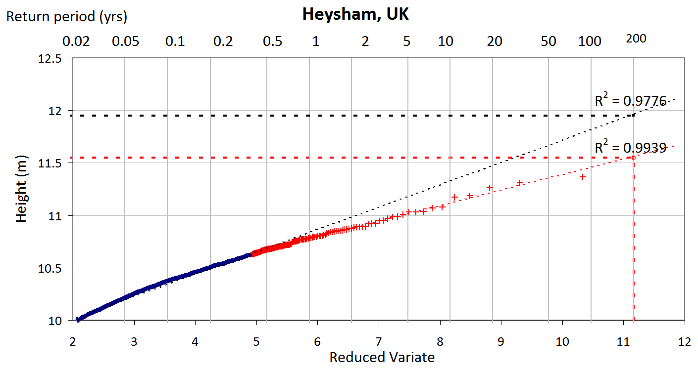
Figure 1 Probability extreme tide plot showing its curvature in a 54-year record. Setting a threshold of 50 greatest extremes tides per year (2439 total), the LSQ intercept is 11.95 m ±0.02 m R²=0.9776 (black). At 5 greatest extreme tides per year (242 points) the straighter red section gives an improved LSQ intercept of 11.6 m (red) ±0.009 m R²=0.9939. Location Heysham UK See Sect. 4.1 and Figs. 2 and 3.

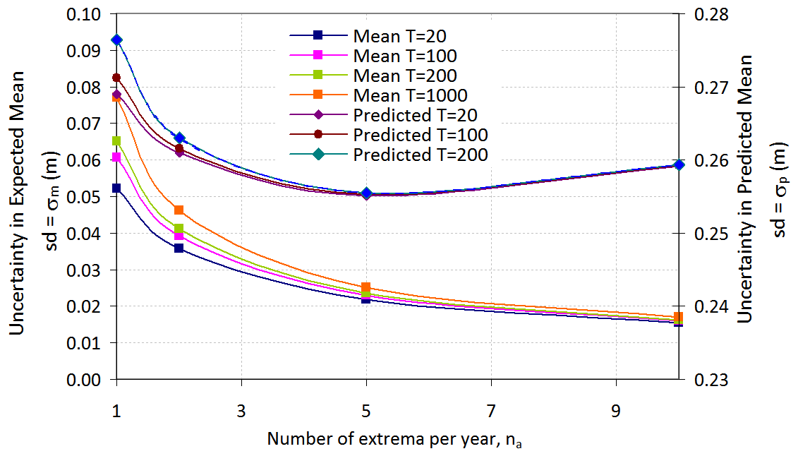
Figure 2 The uncertainty in the expected mean value σ_m and of the predicted new point σ_p plotted against the number of extrema per year n_a for the TMAX method as determined from the tidal data.

3.3 Tide Peak Selection

Clearly, for a duration of tidal data of many decades, the algorithm described above will produce many thousands of peak values. However, only the largest are used because the plot of peak height against the logarithm of return period often deviates away from straight line at lower values of height, such curvature probably being related to shallow water effects during the neap of a spring-neap cycle. Figure 1 demonstrates how such curvature adversely affects the straight line fit. Hence, we use a fit of only the largest n values, since these fall, more or less, in a straight line, where n is calculated from an average number per year, n_A multiplied by the tide gauge record duration in years n_y, i.e. $n=n_{\mathrm{A}}\times n_y$. The optimization of n_A is discussed in Sect. 4.1 and a value of 5 per year seems appropriate. This method is much more convenient than employing a threshold, because the number of maxima selected corresponds directly to the rank number which, as it has been counted with i=1 for the largest, is already known. The above methods for peak detection and peak selection also provide a form of declustering as is now described. We assume here surge durations are generally between a few hours and days (See Batstone et al., 2013; Williams et al., 2016). Firstly, the method selects a single peak in a tidal day, ruling out multiple clusters within the same period. Secondly, surges shapes generally have a single peak with a significant fall from this value within a tidal day (see UK Environment Agency, 2011, Design Surge Profiles). It is therefore extremely unlikely that more than one high tide will coincide with the same surge event and yet still produce a significant extreme value peak. Indeed, as a further check it was tested and verified that none of the final maxima selected (using the given number n_A per year) were found to occur within the same day or on adjacent dates.

The reader may also wish to consider here the similarities between TMAX and the other peak selection methods known as r-largest, AMAX and Peaks Over Threshold (POT). In r-largest, a fixed number of the largest extreme events are selected for each time unit, as opposed to in TMAX where the selection process applies to all of the data. In AMAX, the annual maxima are used. Hence TMAX could be viewed as being similar to AMAX but rather than using an block time of one year, it has a block time of a tidal day. However, unlike AMAX, TMAX incorporates further selections, using the n largest values. The greatest similarity is perhaps with POT, the difference here being that whereas in POT peaks selection is based upon a threshold, in TMAX selection is based upon a given number n, of the largest values. One other general difference is that in the version of TMAX currently described, a simple linear regression is fitted to a logarithmic plot using least squares difference, as opposed to employing generalised Pareto distribution (GPD) as in the other methods.

But what should be the value of N within the TMAX algorithm? If TMAX is considered as a modified form of AMAX, but with a block time of a tidal day, T_D, then N in Eq. (9), rather than representing the number of years of data, becomes the number of tidal days of data. The return period, T_i (in tidal days) then becomes the inverse of Eq. (9), hence

$$\begin{array}{}\text{(12)}& T_i=(N+\mathrm{1})/i\end{array}$$

Incorporating Gringorten's Correction Eq. (10) into Eq. (12) where leads to (in tidal days)

$$\begin{array}{}\text{(13)}& T_i=(N+\mathrm{0.12})/(i-\mathrm{0.44})\end{array}$$

In tests of TMAX, eliminating Gringorten's correction altogether, i.e. using Eq. (12) rather than Eq. (13), was found on average to increase the ESL values by a few centimetres, and increased the 95 % confidence limits slightly by a few millimetres; with AMAX the results were similar, except the 95 % confidence limits were also increases by centimetres. Accordingly, this study utilised Eq. (13) with N specified in tidal days (the block time being one tidal day) and the results being converted to units of years for text and graphical output.

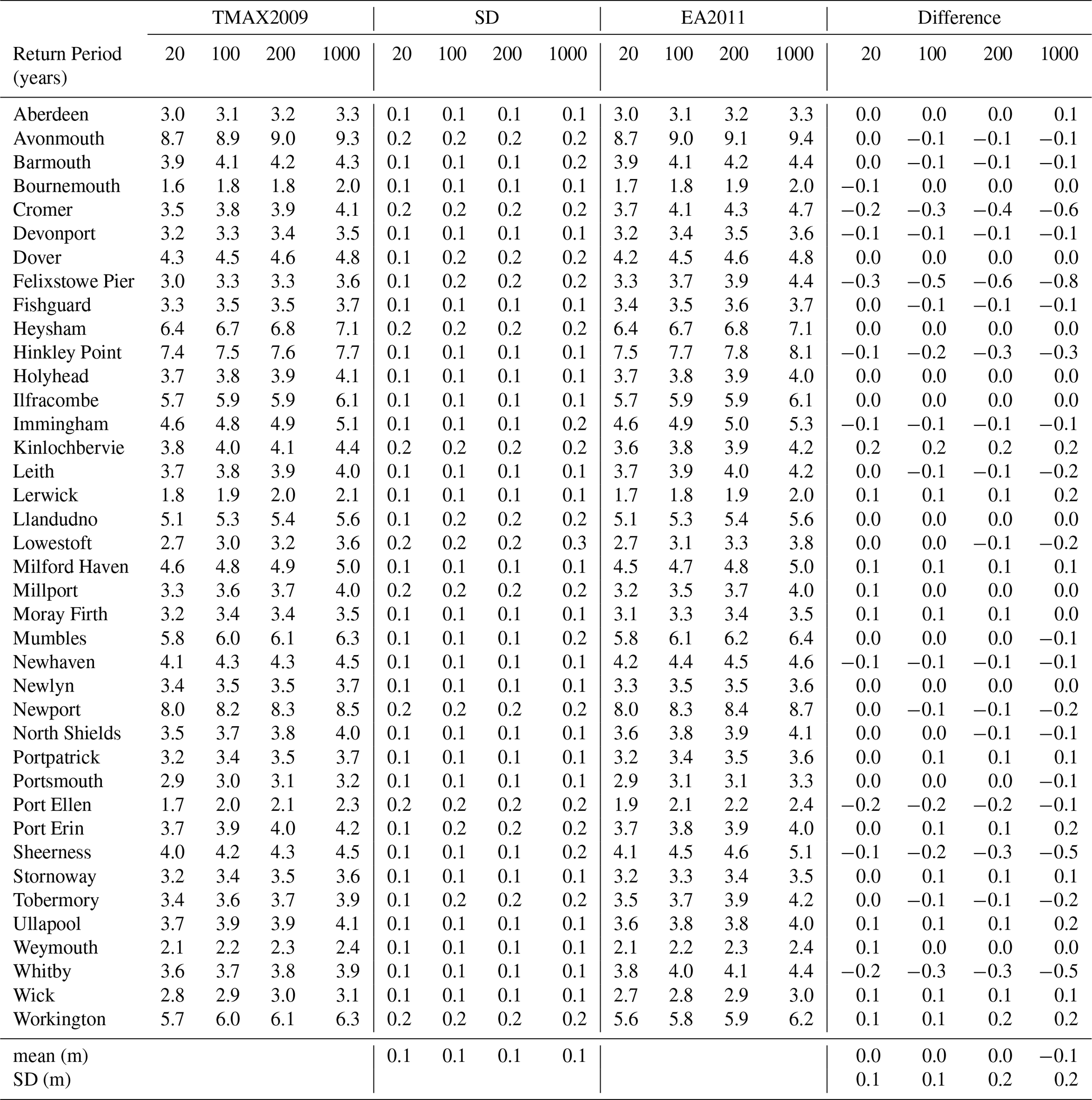
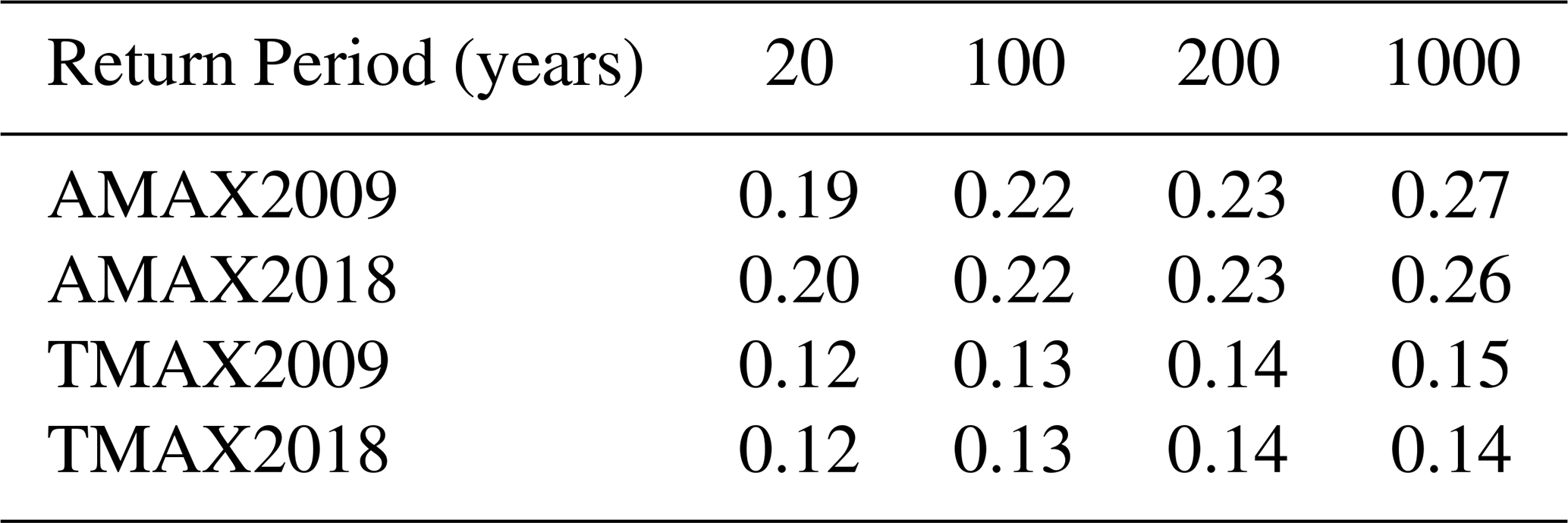
Table 1 ESLs (m) above ODN relative to MSL2008. Results of TMAX2009, Standard Deviation of LSQ fit, Values of EA2011, and Difference TMAX2009-EA2011.

3.4 Straight Line Fit

As discussed above, the ordinary least squares (LSQ) fit, also known as linear regression, was used to determine the line fit (Morrison, 2020). This is despite the existence of many other more complex methods including the Weighted Least Square Rank Regression, method of maximum likelihood estimation (MME), method of moments (MOM), method of L-moments (MLM), method of probability-weighted moments (PWM), the generalized least-squares methods GLSM/V (Coles and Dixon, 1999; Hong et al., 2013; Van Zyl and Schall, 2012). Consideration of these other fitting methods in conjunction with TMAX is viewed as a potential refinement for future research. With both AMAX and TMAX methods, the expected value of a predicted new point (i.e. a flood) is the mean y value of the intersection of the extrapolated regression line with the ordinate corresponding to the required return period. Morrison gives expressions for the mean slope m_m, the mean intercept c_m, the variance of the expected mean ${\mathit{\sigma }}_{\mathrm{m}}^{\mathrm{2}}$ and the variance of the new predicted mean ${\mathit{\sigma }}_{\mathrm{p}}^{\mathrm{2}}$, where n represents the number of data points, x_m, and y_m are the mean x and y values respectively, as

$$\begin{array}{}\text{(14)}& \begin{array}{rl}& {\mathrm{SS}}_{xy}=\sum (x_i-x_{\mathrm{m}})(y_i-y_{\mathrm{m}})\\ & {\mathrm{SS}}_{xx}=\sum {\left(x_i-x_{\mathrm{m}}\right)}^{\mathrm{2}}\\ & m_{\mathrm{m}}={\mathrm{SS}}_{xy}/{\mathrm{SS}}_{xx}\\ & c_{\mathrm{m}}={\displaystyle \frac{(\mathrm{\Sigma }{x}_i{)}^{\mathrm{2}}\mathrm{\Sigma }{y}_i-\mathrm{\Sigma }{x}_i{y}_i\mathrm{\Sigma }{x}_i}{n\mathrm{\Sigma }{x}_i^{\mathrm{2}}-(\mathrm{\Sigma }{x}_i{)}^{\mathrm{2}}}}\\ & s_{y,x}^{\mathrm{2}}=\left(\mathrm{1}/(n-\mathrm{2})\right)\sum {\left(y_i-y_{\mathrm{m}}\right)}^{\mathrm{2}}\end{array}\end{array}$$

$$\begin{array}{}\text{(15)}& {\displaystyle }{\mathit{\sigma }}_{\mathrm{m}}^{\mathrm{2}}=s_{y,x}^{\mathrm{2}}(\left(\mathrm{1}/n\right)+{\left(x_p-x_{\mathrm{m}}\right)}^{\mathrm{2}}/{\mathrm{SS}}_{xx})\text{(16)}& {\displaystyle }{\mathit{\sigma }}_p^{\mathrm{2}}=s_{y,x}^{\mathrm{2}}(\mathrm{1}+\left(\mathrm{1}/n\right)+{\left(x_p-x_{\mathrm{m}}\right)}^{\mathrm{2}}/{\mathrm{SS}}_{xx})\text{(17)}& {\displaystyle }{s}_{\mathrm{d}}={\mathit{\sigma }}_{\mathrm{p}}\end{array}$$

Given the standard deviation, s_d, the predicted value of y at a given value of x_p is given by

$$y=m_{\mathrm{m}}{x}_p+c_{\mathrm{m}}\pm t_{\mathit{\alpha }/\mathrm{2},n-\mathrm{2}}{s}_{\mathrm{d}}$$

where 95 % confidence interval, $t_{\mathit{\alpha }/\mathrm{2},n-\mathrm{2}}$ signifies the t distribution and is commonly taken as approximately two. The variance in the expected mean value is subject only to the distribution of data points, and tends to zero as the number of points increases; whereas the variance in a new estimated point is subjected also to variation in the process under examination, and does not tend to zero as n increases, hence σ_m <σ_p see Eqs. (14) and (15).

3.5 Missing Data

Tide gauge records often contain temporal data gaps due to faulty instrumentation, or damage to the gauge installation. Using the TMAX method, files containing missing tidal data can be accommodated by simply reducing the value of N in Eq. (13) to correspond to the actual number of tidal days of valid data. By contrast, it is not so straightforward in the AMAX or r-largest methods to accommodate missing data, since either synthetic data must be provided to fill the gaps, as was discussed by Gumbel, or whole years of data must be rejected if a significant portion of the annual data content is missing.

4 Comparative Study

The AMAX and TMAX methods were applied to calculate the ESLs for 39 of the 41 UK stations used in the EA2011 study; the difference in number of ports arises because the two stations, Hilbre Island and Exmouth, were not included in the available BODC download. After downloading the tide gauge data, it was first concatenated for each port to form a single data file for each port; these were then imported and manually inspected. Most of the data before 1993 had been recorded at hourly intervals whereas subsequently, data was at 15 min intervals. Although a spline fit had been considered as a strategy to artificially fill-in at 15 min intervals the hourly measurements, it was considered advantageous to use the data directly, especially bearing in mind that the spline fit could itself result in artificial high tide values which had not actually been recorded. Bearing in mind that the TMAX method is dependent upon the height of the recorded peaks rather than their exact timing, the advantage of using much longer records could easily outweigh the potential small inaccuracies induced due to the change in sample rate. In addition, a down-sampling experiment was carried out, by degrading the 15 min periods to hourly sampling. It changed the 200-year ESL by less than 1 cm and the 95 % confidence level by only 1–2 mm. Therefore, to obtain the longest data duration possible, both 15 min and one-hourly data were used within a single file if necessary. Each file was examined for tide gauge malfunctions; any data suspected of being faulty was deleted. Such malfunctions are apparent in the data in a number of ways. Firstly, isolated non-contiguous points consisting of one or more data points, significantly away from the main trend were removed. Secondly, any steady drift of values lasting periods of hours or days e.g. gauge drifts and gauge slips, were removed. Thirdly, sequences of fixed values consisting of several points of exactly the same value were removed, Finally the maximum 5 values in each file were re-checked to verify that the peaks represented a surge and not intermittent tide gauge faults.

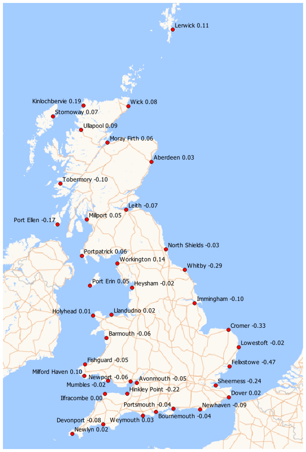
Figure 3 Difference (m) between EA2011 and TMAX2018 for 100 Year ESL.

4.1 Optimising the average number of peaks per year

As discussed above, selecting only the highest peaks avoids the graph curvature of Fig. 1, improving its accuracy. Therefore, although larger sample values are generally associated with a decrease in variance, in this case the opposite may be true. Figure 2 shows the variation of, the uncertainty of the mean, σ_m, and uncertainty of a predicted new point, σ_p , as determined using Eqs. (14) and (15), with n_A, the average number of extremes selected per year, indicating σ_p attains a minimum at a value of n_a of around five extremes per year. This concurs with the value of five per year found by Robson and Reed (2008) for extreme river flow studies and used by Smith (1986), although this may be coincidental. Nevertheless, since we obtain a minimum variance at the value of n_a=5, this was adopted for all subsequent results.

4.2 Analysis

For compatibility with Batstone et al. (2013), all data was sea-level rise de-trended, using the constant value and date origin adopted in that study of 2 mm yr⁻¹, with zero being applied on 1 January 2008. The final date of the data used for the UK Environment Agency study was listed in Table A.1.3 of EA2011 as 1 January 2009. Therefore this comparison study was carried out using tidal data records which were truncated to 1 January 2009. This was repeated for both AMAX and TMAX methods which are referred to here as AMAX2009 and TMAX2009. During the analysis the peak selection algorithm as described above was used. The number of valid days of data was determined and only those in the top rank corresponding to a total number, n, corresponding to n_a of 5 per year were used. The peaks were ranked and plotted using Gringorten's formula. The LSQ regression analysis was then used to give an intercept for the required return periods. The entire analysis was repeated using the complete data set to 1 May 2018, being referenced as AMAX2018 and TMAX2018. Unfortunately, a later update was not available at the time of carrying out this study. The periods from tidal days to years were converted as required. The results were derived solely from the tide gauge data and have not been re-processed in any other way. Comparisons with the results from EA2011 are indicated where appropriate.

Table 2 Mean of Standard Deviation (m) for AMAX and TMAX based upon variance in predicted level, σ_p of the LSQ fit.

4.3 Results

Table 1 compares the results of TMAX2009 with EA2011, displaying ESLs in metres above ODN relative to MSL2008 for all 39 ports. The results are shown for each of the return periods of 20, 100, 200, and 1000 years. The column headed SD shows standard deviation for the TMAX2009 ESLs as obtained from the Least Squares Fit using Eq. (16). The column headed “Difference” shows the values returned from TMAX2009 minus those from EA2011. The lower two rows show the mean values and their standard deviations. The mean differences were of the order of centimetres while the standard deviations were of the order of 10 to 20 cm, with both rising for the longer return periods. Figure 3 shows the estimated ESL values for a 100-year return period at 39 UK sites on a map as derived from TMAX2018 rather than from TMAX2009, utilising all of the tidal data examined. The results are discussed in the error analysis in the following section.

4.4 Error Analysis

Table 2 shows the standard deviation for each given return period as calculated from the best fit to the source “n” maxima, plotted using Eqs. (8) and (13) and evaluated from those equations listed in Sect. 3.4. The standard deviation is calculated from the expected variance in a new forecast point σ_p Eq. (15) rather than the smaller variance in the mean σ_m Eq. (14), as indicated in Sect. 3.5. It can be seen that there is a significant difference between the standard deviation for the two methods AMAX and TMAX, with TMAX significantly outperforming AMAX, reflecting the larger number of points involved in the TMAX method. On average the standard deviations for TMAX were approximately 60 % of those of AMAX which suggest a useful margin of improvement in accuracy. The level of agreement between AMAX and TMAX with the results of EA2011 are now described.

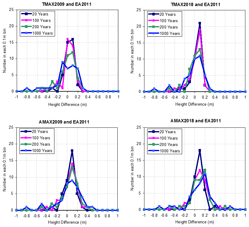
Figure 4 Differences in ESL between TMAX and EA2011 and between AMAX and EA2011 using data to 2009 and 2018.

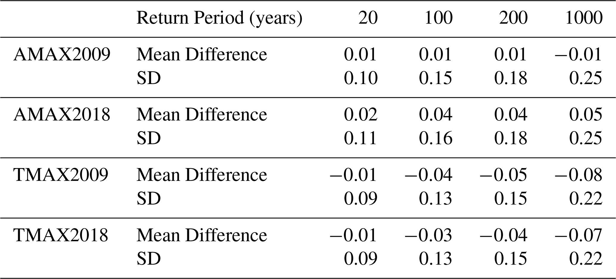
Table 3 shows the mean differences in ESL, and standard deviations of the differences between TMAX and EA2011 and between AMAX and EA2011, while Fig. 4 shows the differences as histograms. With AMAX the mean of the differences was generally slightly positive, indicating marginally higher ESLs as compared to EA2011, whereas with TMAX the ESLs were generally lower, indicating a slight reduction in sea-defence requirements. For AMAX the mean differences were slightly smaller than TMAX, indicating marginally better agreement, perhaps reflecting the use of AMAX in EA2011 at those locations where SSJPM was not used. However, the standard deviation of the difference was much greater than the mean difference, for all return periods listed. The standard deviation of the difference ranged from 0.09 m for the 20-year return period with TMAX2009/2018 to 0.25 m for the 1000 years return period with AMAX. The Students “t” test was used establish the significance of the mean difference values, (α=0.05, 39 pairs, df=38 tails =2), giving a critical value at a 95 % confidence level of t_crit=2.02. Out of sixteen comparisons made, fifteen determined “t” to be considerably smaller than this critical value, the exception being AMAX09 at a 1000-year return period where only a marginal significance was found. Thus, according to the paired t-test the values of the mean difference is not significant. Across all studies for TMAX2009, TMAX2018, AMAX2009 and AMAX2018 and their comparison with EA2011 there were no consistent positive outliers exceeding two standard deviations above the mean. However, there were consistently significant negative outliers, with over two standard deviations below the mean; these were Cromer, Felixstowe and Sheerness. Significantly, these ports had been singled out for discussion of levels in the EA2011 study. The port of Felixstowe consistently gave return levels having the largest significant difference from those of EA2011. A further study using TMAX of tidal records for the nearby port of Harwich, at a distance of only 3 nautical miles from Felixstowe, gave a considerably improved level of agreement of ESLs with the results of EA2011 for Felixstowe, although the implication of this are not clear.

Table 3 Standard Deviation in Mean and Mean Difference between AMAX and EA2011 and between TMAX and EA2011 (m).

5 Conclusions

The paper describes a method named here as “TMAX”, which is designed to derive extreme sea level statistics (ESLs) from tide gauge data, based upon a modification of Gumbel's method of 1954. When compared with the AMAX method, TMAX confidence bounds are approximately 40 % smaller than those for AMAX, suggesting a significant margin of improvement in accuracy. Further, it is shown that TMAX generates estimates of ESLs which are in broad agreement when compared with those published by UK Environment Agency 2011 (EA, 2011) at all 39 locations, and good agreement at 36 locations, with agreement at 3 locations in the southern North Sea, in particular at the port of Felixstowe, being outliers. Overall mean differences between the two methods were of the order of centimetres and standard deviation of the order of decimetres. However, the TMAX method is much simpler than the SSJPM used in EA2011. Unlike in the EA2011 study, where one quarter of sites were singled out for special attention, the same algorithm was used at each location without “manual intervention”. Also, unlike the SSJPM, the TMAX assumes a Gumbel Type 1 statistic and does not split the tide into two components, i.e. the predicted tide and skew tide. Hence it does require (a) harmonic tidal analysis, (b) the use of a probability density function, or (c) the fit of a generalized Pareto distribution (GPD) and therefore does not suffer from any errors induced by these processes, which may, in a minority of cases, significantly influence the accuracy of the result. A further advantage of the TMAX method is that missing data, quite common in tide gauge records, is handled in a simple, efficient and elegant way. This study of 39 UK locations indicates that the TMAX method shows promise as a general screening method for extreme sea level analysis. It is hoped to extend this study to provide a world-wide comparison as new databases become available. The approach has the potential to facilitate the generation of ESLs directly from tide gauge data, thereby informing and improving strategies for coastal management and resilience.