Monsoons, plumes, and blooms: intraseasonal variability of subsurface primary productivity in the Bay of Bengal

During the southwest monsoon, seasonal storms bring torrential rainfall to the South Asian subcontinent and the northern Indian Ocean. Dense cloud cover limits the amount of sunlight that reaches the ocean surface, and sediment-laden river runoff limits the depths to which light can penetrate. Changing light availability should affect phytoplankton primary productivity and its dependent biogeochemical processes, yet little is known about how subtropical weather is linked to ecosystem processes below the ocean’s surface. Here, using novel physical and bio-optical measurements from an array of free-drifting, autonomous systems in the Bay of Bengal, we show that the onset of cloudy conditions associated with “active” monsoon conditions led to >50 % reduction in gross chlorophyll productivity (GCP) near the subsurface chlorophyll maximum (SCM) relative to sunny “break” conditions. Optical backscatter measurements confirm chlorophyll fluorescence fluctuations correspond to biomass variability of a similar scale. Simultaneous bioacoustic measurements collected onboard the autonomous platforms suggest this intraseasonal variability in SCM chlorophyll and biomass generated a response in higher trophic levels. Long-term measurements from biogeochemical (BGC) Argo floats in the bay confirm the presence of intraseasonal oscillations in chlorophyll a concentration with days-to-weeks variability in magnitude similar to the regional annual cycle in the region. Our findings demonstrate that intraseasonal subtropical air-sea variability modulates important regional biogeochemical ocean processes in the Northern Indian Ocean with implications for the Indian Ocean carbon cycle.

1 Introduction

The ocean contributes roughly 50 % of total global autotrophic carbon fixation, with more than 40 % of ocean primary productivity occurring in vast but relatively low biomass oligotrophic seas (Antoine et al., 1996). Our current understanding is that net primary productivity in the subtropical oligotrophic ocean is limited by nutrient supply and not light availability (Mignot et al., 2014), but recently developed autonomous long-duration measurements of subsurface processes allow a more comprehensive analysis of the subsurface variability than has previously been possible (Johnson and Bif, 2021). Less is known about how subtropical primary productivity varies on small time- and space-scales, or its response to the rapidly changing subtropical weather patterns.

Current generation coupled atmosphere-ocean numerical models lack fidelity on 10–90 d timescales in the tropics and subtropics (Gadgil et al., 2005; Mandke et al., 2020; Shroyer et al., 2021). This so-called intraseasonal variability is a major component of global weather and is fundamental to predicting climate phenomena like the South Asian monsoon (Shroyer et al., 2021). How intraseasonal fluctuations impact biogeochemical processes in the subtropical ocean is poorly understood (Hansell, 2009). Since coupled ocean-atmosphere models struggle to accurately represent the magnitude or the timing of intraseasonal fluctuations (Gadgil et al., 2005; Mandke et al., 2020; Shroyer et al., 2021), these fluctuations must also be inaccurately represented in coupled biogeochemical models. Intraseasonal oscillations like the Madden-Julian Oscillation or the Monsoon Intraseasonal Oscillation impact much of the subtropical ocean, so the potential impact on biogeochemical processes may be significant.

Satellite observations reveal the decrease in surface productivity during the southwest monsoon (approximately June to September) in the Bay of Bengal due to the impact of monsoon weather on light availability at monthly scales (Kumar et al., 2010a, b). Light availability at the surface decreases via a reduction in shortwave radiation during the southwest monsoon (Weller et al., 2016), which oscillates at 10–90 d timescales, categorized as the sunny “break” period and rainy and cloudy “active” periods of the monsoon (e.g., Shroyer et al., 2021). Subsurface light availability additionally decreases due to the increasing diffuse attenuation following river run-off, where monsoon rain events inject high concentrations of sediments into the bay, even 𝒪(100 km) from the coastline (Kumar et al., 2010a). The weather systems that reduce shortwave radiation also impact ocean color satellite measurements, so satellite measurements cannot observe biogeochemical processes over the entire intraseasonal oscillation. The subsurface impacts of intraseasonal varying light availability are generally unknown, contributing to the uncertainty in our understanding of the Indian Ocean carbon cycle. In particular, stratification, vertical salinity gradients and barrier layers have a dominating influence on subsurface biomass in the Bay of Bengal (Prasanth et al., 2023).

Autonomous technology to measure biogeochemical variability in the ocean – such as the BGC-Argo float program (Argo, 2000) – has provided new opportunities to quantify the variability of the ocean carbon system (Mignot et al., 2014; Johnson and Bif, 2021). These platforms provide information about biogeochemical transformations below the ocean's surface that are largely invisible to satellite remote sensing (Mishra et al., 2005). Although only recently deployed at scale, autonomous biogeochemical measurements have demonstrated that our capacity to make future predictions of the state of the climate depends sensitively on constraining biogeochemical ocean processes (Gray et al., 2018; Johnson and Bif, 2021).

The BGC-Argo float program typically samples at weekly time scales, which is sufficient to describe the intraseasonal biogeochemical variability but not diel processes, such as nonphotochemical quenching (NPQ) and the diel cycle in phytoplankton biomass. Near the surface, NPQ results in a non-biomass-related diel reduction in chlorophyll a (Chl) fluorescence under high light conditions (Müller et al., 2001). In contrast, the diel cycle is distinct from NPQ in that concentrations of Chl (Marra, 1997; Prasanth et al., 2023), dissolved oxygen (Nicholson et al., 2015; Barone et al., 2019), and particulate carbon (White et al., 2017) increase with increasing irradiance. The diel cycle results from the competing processes of day-time gross primary production (GPP) and day- and night-time respiration and grazing losses (Marra, 1997). The tight coupling between the diel cycle and the solar cycle (i.e., sunrise and sunset) has allowed the development of robust methodologies for estimating GPP and loss rate for a range of biological variables (Marra, 1997; Nicholson et al., 2015). Although the diel cycle directly results from the diel variability in subsurface irradiance, the sensitivity of the diel cycle to the short-term cloud- or turbidity-driven changes in irradiance remains under-explored.

An improved understanding of the Indian Ocean carbon cycle and its sensitivity to intraseasonal oscillations not only requires a better understanding of primary productivity but also the effect on higher trophic levels. Currently, most autonomous platforms like BGC-Argo deployed long-term do not observe grazers due to the difficulty in making accurate observations, either directly or indirectly. Acoustic backscatter measurements at high frequencies (i.e., 1 MHz) are sensitive to smaller zooplankton species, including grazers, as compared to lower frequency measurements of acoustic backscatter traditionally used to identify fish and larger marine organisms (Lavery et al., 2007; Ohman et al., 2019; Gastauer et al., 2022). However, without confirming net or video observations (e.g., Lavery et al., 2007), these bioacoustic or high-frequency acoustic backscatter observations (as we present here) remain a relatively uncertain representation of grazer variability.

Here we report on physical, bio-optical, and bio-acoustic measurements gathered in the Bay of Bengal during the 2019 monsoon season, described in the next section. We then quantify the impact of ocean clarity and passing monsoon storms on subsurface irradiance, and we statistically relate fluctuations in gross production to the subsurface irradiance. We contextualized our observations with an analysis of longer-term BGC-Argo measurements. Finally, we conclude by discussing some of the wider implications of our results, including regional patterns in subsurface productivity we may infer from our results, and evidence of higher trophic level variability. Taken together, our results demonstrate the variability in biogeochemical quantities on intraseasonal time scales, and show how increased autonomous observational capacity can contribute to our understanding of the processes that shape the ocean climate system.

2 Materials and methods

2.1 Field campaign

As part of a campaign to study intraseasonal oscillations in monsoon weather, we deployed an array of three densely instrumented buoys and ocean-wave-powered Wirewalker profiling vehicles (Pinkel et al., 2011) that gathered physical, bio-optical, and irradiance measurements in July 2019 in the Bay of Bengal. Each Drogued Buoy Air-Sea Interaction System (DBASIS) was deployed for ∼19 d (Fig. 1): M1 on 9 July, M2 on 10 July, and M3 on 11 July, generally following the mesoscale flow. Each profiler had a metocean buoy on the surface, a vertically profiling Wirewalker over the upper 100 m (Pinkel et al., 2011), and six X-wings (1 m² drag elements) over 200 to 210 m depth so that the system drifted with the subsurface currents at 200 m. They collected approximately 200 profiles per day spanning the upper 100 m of the water column with sub-meter vertical resolution.

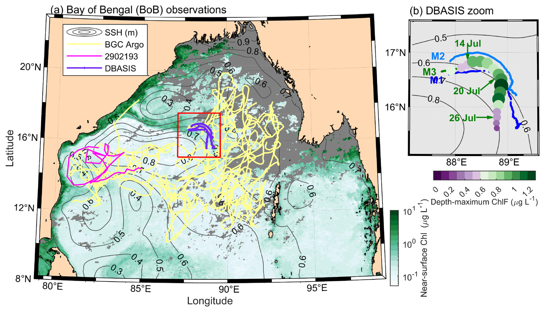
Figure 1 Overview of observations. (a) Bay of Bengal with the study region (red square), location of analyzed biogeochemical (BGC) Argo profilers deployed from 2013 to 2018 (yellow, WMO ID: 2902086, 2902087, 2902114, 2902158, 2902160, 2902161, 2902189, 2902196, 2902217, 2902264), with a further analyzed 2016 profile highlighted (pink, WMO ID: 2902193; Argo, 2000), location of DBASIS profilers (purple), 5 d averaged (10–15 July 2019) satellite chlorophyll (Chl, background color; Sathyendranath et al., 2019, 2023), and gray contours of the EU Copernicus Marine Service global ocean $\mathrm{1}/\mathrm{12}$° sea surface height (SSH, 4 July 2019; https://doi.org/10.48670/moi-00021). (b) Position and date for the three high-resolution DBASIS floats: M1 (dark blue), M2 (light blue), and M3 (green), with the depth-maximum chlorophyll a fluorescence (ChlF) shown for M3 at noon each day. Gray contours show SSH (m). DBASIS floats were located in depths ∼2600 m deep and ∼400 km southeast of the nearest coastline.

The buoy's meteorological package measured wind (2.9 m a.m.s.l. – above mean sea level), air temperature (2.6 m a.m.s.l.), humidity (2.6 m a.m.s.l.), precipitation (2.9 m a.m.s.l.), barometric pressure (2.3 m a.m.s.l.), sea surface temperature (0.3 and 1.5 m b.m.s.l. – below mean sea level), and downwelling solar and infrared radiation (3.2 m a.m.s.l.). The metocean buoys were equipped with Kipp and Zonen SMP21 shortwave radiation sensors that measure downwelling radiation over wavelengths of 285 to 2800 nm (50 % points). These measurements were used to estimate the surface photosynthetically available radiation (PAR).

We equipped the Wirewalker profilers with RBR Inc. conductivity, temperature, and depth (CTD) sensors augmented by SBE Wetlabs Ecopucks measuring Chl fluorescence (ChlF, a proxy for Chl biomass), optical backscatter at 532 nm, and chromophoric dissolved organic material (CDOM; not used in the analysis presented here). We measured subsurface downwelling irradiance onboard the Wirewalkers using a Satlantic OCR-504 multi-spectral radiometer at four bands, 380, 412, 490, and 532 nm. All parameters were collected continuously at 6 Hz and telemetered at that resolution in real-time via RUDICS Iridium modems on the surface buoy. Using the factory calibration, we convert the optical backscatter to Nephelometric Turbidity Unit, τ (NTU). The median time between profiles was 10 min at M2 and M3 and 20 min at M1. For all quantities, we only use measurements during the smooth upward ascent of the profiler.

To estimate the diffuse attenuation averaged by depth, K_d (m⁻¹), the raw measurements of downward irradiance were grouped in time and depth into 3 h and 4 m bins, respectively, and then least-squares fitted to an exponential curve. Irradiance was then interpolated back to the original 𝒪(10 min) time resolution (see Supplement for further details).

We also equipped the profilers with a downward-looking Nortek Signature with a frequency of 1 MHz, from which we show only the acoustic backscatter (Zheng et al., 2022). For each profiler's upcast, we averaged the acoustic amplitudes of each of the four beams over the first 20 bins (2.5 m depth range) closest to the transducer. We then interpolated range-averaged beam amplitudes onto a 0.25 m uniform depth grid before averaging all four beams. The 1 MHz backscatter was similar to the R/V Sally Ride acoustic backscatter that had a frequency of 150 kHz, with differences between frequencies as expected from literature (Lavery et al., 2007; Ohman et al., 2019; Gastauer et al., 2022).

All three DBASIS floats had the same bio-optical instrumentation and generally collected comparable measurements. We present time series from only M3 here, which collected continuous (unlike M1) and high resolution (10 min) data, and show M1 and M2 observations in the Supplement. Our key results and findings were similar for all floats.

2.2 Chlorophyll a fluorescence

The primary objective of the field campaign was to investigate air-sea interactions and the underlying physical variability in the BoB. As such, while biogeochemical observations were collected autonomously, we did not sample water in order to field calibrate the chlorophyll sensors. Instead, using laboratory calibration carried out just prior to the experiment, we converted the observed ChlF in relative fluorescence units (RFU) to real units (µg L⁻¹) via $\mathrm{ChlF}=\mathrm{0.012}\times (\mathrm{RFU}-\mathrm{50})$. This conversion has an unknown uncertainty that linearly scales for all values (i.e., percentage error). For context, the observed surface ChlF from the drifting systems and MODIS-Aqua surface Chl from July 2019 were 0.17 and 0.33 µg L⁻¹, respectively, with these points located an average of 54 km apart. The focus of our work is not on the absolute quantities of ChlF but rather on their response to surface and penetrative solar radiation, so we focus on the robust trends in co-variability rather than absolute values.

Chlorophyll pigment concentration, ChlF, and phytoplankton biomass (i.e., carbon content) are highly variable under changing light conditions as phytoplankton adapt to changing light environments by adjusting their light-harvesting pigments (Cullen, 1982, 2015). Due to this, estimates of biomass from backscatter observations are typically a more robust estimate of carbon biomass than ChlF. However, in the situation encountered here, non-algal sources of backscatter at-times confounded measure of algal concentrations, for example in the high-sediment coastal waters we observed at M3 before 15 July (Fig. 2d). Focusing only on times when the backscatter signal was due to algal diel variability, ChlF and backscatter variability was similar. This analysis showed that ChlF was a good proxy for phytoplankton biomass at the depth of the subsurface chlorophyll maximum (SCM), which we discuss throughout the manuscript.

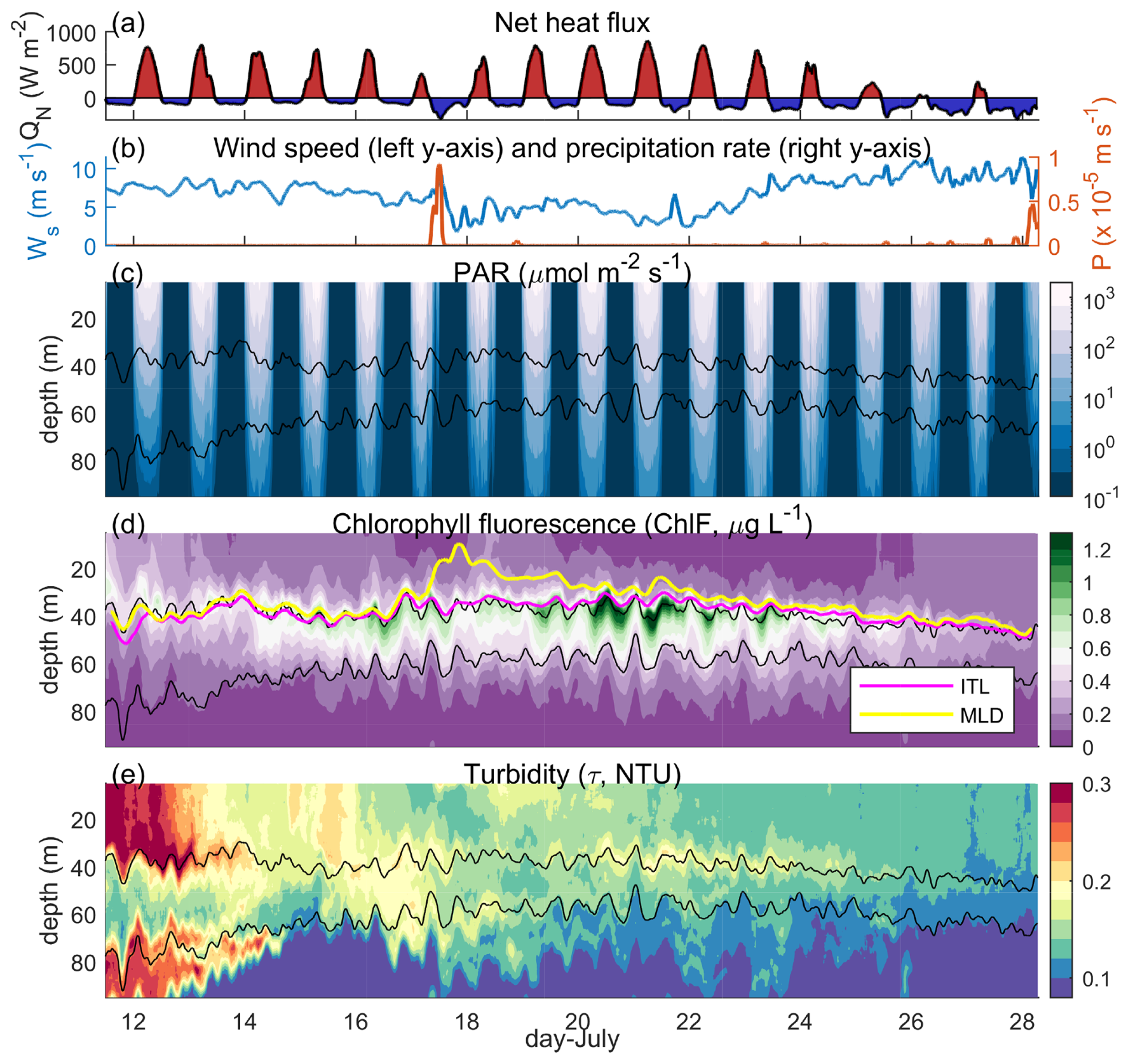
Figure 2 Observations at M3. (a) The net heat flux (Q_N), (b) wind speed (blue left y axis, W_s) and precipitation rate (orange right y axis, P), (c) photosynthetically available radiation (PAR), (d) ChlF, and (e) turbidity (τ). In (c) to (e), two isopycnals (1021.5 and 1023 kg m⁻³) are contoured (black), and in (d) the depth of the isothermal layer (ITL, pink) and mixed layer depth (MLD, yellow) are shown.

Near the surface, non-photochemical quenching (NPQ) results in a non-biomass-related diel reduction in fluorescence under high light conditions (Müller et al., 2001). To correct for NPQ in the ChlF measurements, we follow methods established for other rapidly profiling platforms (Davis et al., 2008; Todd et al., 2009; Schlosser et al., 2022). We least-squares fit irradiance at 490 nm to ChlF over the upper 20 m over 1 d windows, stepping in time every 0.1 d and averaging overlapping time steps. We set a maximum correlation coefficient of −0.1, ensuring we only modify ChlF if ChlF decreased when irradiance increased. Although we used only ChlF over the upper 20 m for the least-squares fitting, we corrected ChlF for all depths with non-zero irradiance. The NPQ correction to ChlF was small, with a 95th percentile of 0.016 µg L⁻¹. Further details are available in the Supplement.

At all profilers, the depth of maximum ChlF was identified within a narrow density range. Excluding the initial 2 d observed at M1 (see Supplement), the SCM and the 1021.5 kg m⁻³ isopycnal were significantly correlated (r²=0.85, p<0.001) with a mean absolute error of 1.65 m. By defining the SCM as the depth of the 1021.5 kg m⁻³ isopycnal ±1 m, the SCM can be matched to an along-isopycnal reference frame. Given the internal wave fluctuations (∼15 m) observed during the campaign, employing an along-isopycnal reference frame was convenient for isolating the impact of changing surface irradiance and diffuse attenuation on ChlF at the SCM (denoted ChlF_SCM). The 1021.5 kg m⁻³ isopycnal had an average depth of 39 m at M3 (Fig. 2) that deepened to 50 m at M1.

2.3 Diel cycle method

ChlF and integrated ChlF reflects the standing stock of chlorophyll, and therefore integrates pigment concentration over days to weeks. To understand the rate at which ChlF is produced and lost due to the local conditions at the SCM, we applied the diel cycle method (Nicholson et al., 2015; Barone et al., 2019). We identify the rate of gross ChlF production (GCP_SCM) and ChlF loss (code available at https://github.com/duebi/dielFit, last access: February 2020) to the NPQ corrected ChlF_SCM. This loss term describes all processes resulting in a reduction of ChlF_SCM, including grazing, mortality, and downward export.

The diel cycle method linearly fits three terms via ordinary least-squares fitting to ChlF_SCM. This allows us to directly evaluate the response of SCM production to intraseasonally modulated PAR, rather than relying on changes in the accumulated concentration. We note that when deciding the depth region to vertically average ChlF_SCM over (2 m), averaging a larger depth range decreased the effectiveness of the diel cycle fit (i.e., the correlation coefficient decreased and mean absolute error increased). The three fitted terms in the diel cycle method included a constant, a constant loss rate for both day and night, and a variable in time GCP_SCM rate similar to the clear-skies PAR, with day-time growth maximum at noon and a zero rate of change at night.

Since we collected radiation measurements, we did not need to simulate the solar cycle. We modified the code to optionally include the observed PAR at the SCM (denoted PAR_SCM) to model growth (henceforward referred to as the PAR_SCM method). The PAR_SCM method is similar to the sinusoidal growth model but accounts for the impact of cloudiness, changes in diffuse attenuation, or perturbations of the SCM depth on growth. Before fitting to ChlF_SCM, we integrated each growth scheme in time. For all three profilers and days sampled, we fit each 26 h period (starting at 23:00 LT), overlapping each day by 1 h. We additionally modified the diel cycle methodology so that the fitted GCP_SCM and loss is always positive.

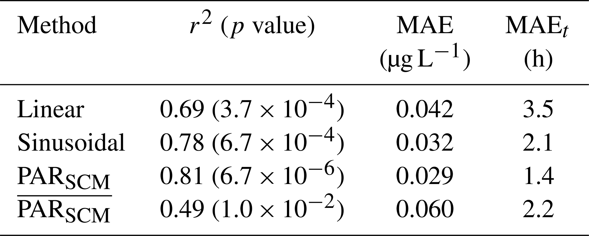
The performance of the fit was assessed by estimating the correlation coefficient and the mean absolute error, $\mathrm{MAE}=\mathrm{1}/n\sum \left|\right|{\mathrm{ChlF}}_{\mathrm{SCM}}-{\mathrm{ChlF}}_{\mathrm{fit}}\left|\right|$, where ChlF_SCM is the observed ChlF at the SCM, ChlF_fit is the diel cycle fit, and n is the number of samples. Of the tested linear, sinusoidal, and PAR_SCM schemes for GCP_SCM, the PAR_SCM method consistently returned the smallest MAE and better predicted the timing of the observed ChlF_SCM maxima by 45 min on average across all floats (Table 1). The sinusoid method also returned a good fit, with a larger MAE, but the linear method was relatively poor in describing the observed ChlF_SCM variability. The fitted mean absolute error doubled when fitting ChlF at a constant depth rather than along-isopycnal due to the vertical heaving of the SCM by passing internal waves (i.e., ChlF_SCM; Table 1). The fitting routine was also effective at M1 and M2. At M1, the timing of peak afternoon ChlF_SCM was more variable, particularly when large-amplitude internal waves deepened the SCM during the day (see Supplement). We also applied the above diel cycle fitting methodology to turbidity to estimate gross turbidity production (GTP_SCM) and turbidity loss. We computed the confidence intervals of the model by bootstrapping the residuals with 200 iterations (Nicholson et al., 2015; Barone et al., 2019).

Table 1 The performance of the diel cycle fit averaged over all three profilers and days fitted. We tested three methods of estimating the gross chlorophyll production (GCP) along an isopycnal (1021.5 kg m⁻³) estimated as the subsurface chlorophyll maximum (SCM): linear, sinusoidal and from the observed PAR_SCM. We also applied this method at a fixed depth corresponding to the average depth of the SCM at each profiler, labeled $\stackrel{\mathrm{‾}}{{\mathrm{PAR}}_{\mathrm{SCM}}}$ where $\left(\stackrel{\mathrm{‾}}{\cdot }\right)$ indicates an average in time. We show the estimated correlation coefficient (r²) and mean absolute error (MAE) from fitting ChlF, and we estimate the MAE in the timing of maximum ChlF (MAE_t).

2.4 BGC-Argo analysis

To contextualize our observations and investigate the frequency of light-limited productivity at the SCM in the bay, we analyzed 12 BGC-Argo floats deployed in the BoB, obtained via the OneArgo-Mat routine (Frenzel et al., 2020). These floats were equipped with a CTD and bio-optical sensors (WET Labs ECO-FLBB AP2 or MCOMS, see  Johnson et al., 2017) measuring temperature, salinity, pressure, chlorophyll fluorescence (ChlF), optical backscatter coefficient at 700 nm (at ∼124°), as well as other sensors not used here. The data were quality controlled using standard Argo protocols (Wong et al., 2022) and processed following Uchida et al. (2019). Quality-controlled data was used when available (quality flags 1, 2, 5 or 8), else visual inspection and simple outlier removal was performed (quality flags 0 or 3).

The raw signals were converted to ChlF (µg L⁻¹) and particulate backscattering coefficient (m⁻¹) following BGC-Argo procedures (Schmechtig et al., 2018). To account for variations between sensors, we standardized the minimum ChlF and backscatter value by removing the median “dark” or background value at pressure > 600 dbar for each float (Uchida et al., 2019). BGC-Argo floats vary in their temporal and vertical sampling frequencies, so following Uchida et al. (2019) we interpolated the quality-controlled float data onto uniform temporal grids with time steps equal to the minimum temporal sampling rate, which is 10 d for most floats. We standardized the vertical grid from 4 to 1000 m. It had 2 m resolution in the upper 300 and 10 m resolution below that. This interpolation was performed using a hermite polynomial scheme (pchip in Matlab), but depths outside the observed range were excluded (i.e., no extrapolation). We applied a 3-point moving-median in the vertical to remove measurement noise and aggregates.

The BGC-Argo subsurface ChlF was also maximum near a consistent isopycnal, like the DBASIS observations, except ChlF was maximum near the 1022 kg m⁻³ isopycnal, so we defined this isopycnal as the SCM depth. Individual months could have enhanced ChlF near a slightly different isopycnal, like the 1021.5 kg m⁻³ isopycnal used when analyzing the DBASIS floats, but we simply use the same isopycnal year-round. To estimate the ChlF_SCM, we averaged ChlF over the 10 m above and below this depth. Since the floats profile once every 10 d, and there are too few floats to apply more advanced statistical techniques (Johnson and Bif, 2021), we cannot estimate GCP_SCM from diel cycles for the BGC-Argo data. Instead, we examined the floats for any evidence of a correlation between ChlF_SCM and PAR at the surface and SCM (described below). We note the diel cycle in ChlF_SCM is prevalent in the Bay of Bengal (Lucas et al., 2016) and has the potential to alias multi-day trends in ChlF if measurements of ChlF are taken at different local times, as is the case for BGC-Argo measurements. To avoid this aliasing, in regions with diel cycles, ChlF and other biological or bio-optical variables should be measured at similar times of the day.

2.5 Satellite and reanalysis data

To understand the co-variance of light and BGC-Argo observed ChlF, we considered both MODIS Aqua PAR (NASA Goddard Space Flight Center and Ocean Ecology Laboratory, 2018) and the atmospheric reanalysis ECMWF Reanalysis v5 (ERA5) product (Hersbach et al., 2018). On average, the PAR estimated at M3 was less than the satellite derived estimate but similar to the ERA5 estimate. We thereby estimated surface PAR from the ERA5 shortwave radiation, by dividing shortwave radiation by 2.114 (Britton and Dodd, 1976). Then, to estimate PAR at the SCM, we utilized the 490 nm diffuse attenuation (K_d490) from the monthly averaged MODIS-Aqua (Goddard Space Flight Center and Ocean Ecology Laboratory, 2018a) and converted to a PAR equivalent using the relation in Morel et al. (2007). If this data was missing due to cloud cover, we took the monthly climatology value instead. For a short-term estimate of 490 nm diffuse attenuation (K_d490) at the start of our DBASIS time series, we analyzed the Ocean Color CCI (OC-CCI) merged satellite product, which had a spatial resolution of 4 km and was averaged over the 5 d period of 10 to 15 July 2019 (Sathyendranath et al., 2019, 2023).

3 Results

3.1 Southwest monsoon campaign

The 2019 field campaign enabled a detailed investigation of the co-variability of subsurface physical and bio-optical properties on an hour-by-hour basis over a nearly 3-week deployment (Figs. 1 and 2). Conditions at deployment were consistent with the southwest monsoon “break” period with weak winds (∼7.5 m s⁻¹), large net heat fluxes into the ocean (Q_N, daily average Q_N of 180 W m⁻²), and no precipitation (Fig. 2).

The DBASIS array was deployed at the intersection of two eddies, as inferred from sea surface height (SSH, Fig. 1). Low-SSH (SSH < 0.5 m) and high-SSH (SSH > 0.5 m) eddies were present to the northwest and southwest, respectively. Between these two eddies, a plume of elevated surface chlorophyll was advected more than 400 km from the coast toward the DBASIS array (Fig. 1a). This coastal plume exhibited elevated turbidity (τ) and surface chlorophyll a fluorescence (ChlF), both of which reduced light penetration into the upper ocean (Fig. 2). Similar coastal plumes have been observed elsewhere at the intersection of cyclonic and anticyclonic eddies (i.e., eddy dipole, Malan et al., 2020).

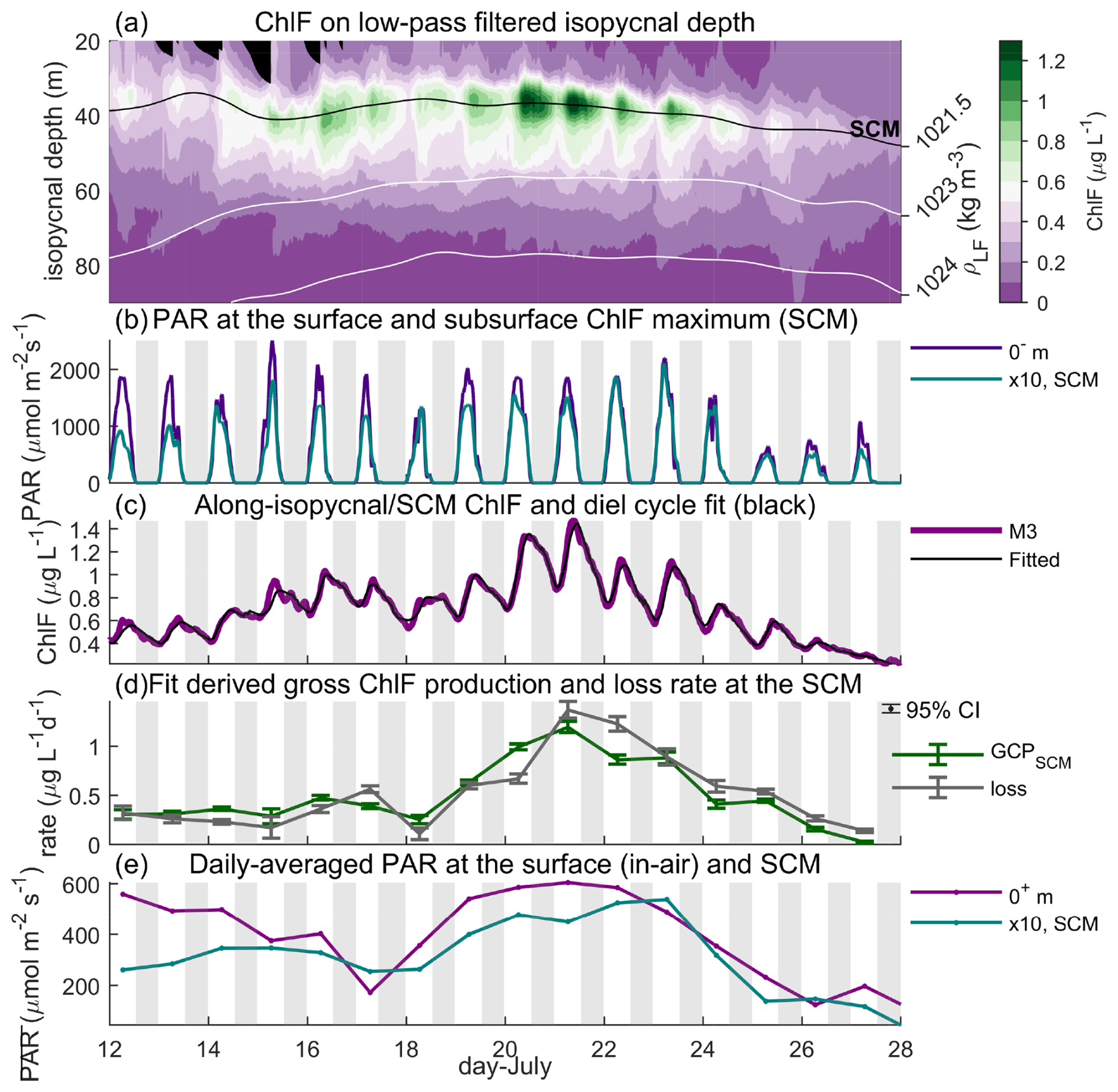
Figure 3 Co-varying light and chlorophyll. At M3, (a) on isopycnal ChlF, with depth representing the 48 h low-pass filtered isopycnal depth (white contour, right y axis) and the SCM depth labeled (black contour). (b) PAR at the surface (purple, PAR₀) and subsurface chlorophyll maximum (SCM, teal, PAR_SCM) multiplied by 10. (c) ChlF_SCM (purple) and the diel cycle fit (black, see “Methods”). (d) Rate of gross ChlF production (GCP_SCM, green) and loss (grey) at the SCM, with the 95 % confidence interval labeled (error bars). (e) Similar to panel (b) but daily averaged (denoted by the over-bar). Note 0⁺ and 0⁻ m indicate surface measurements in air and water, respectively, and we denote a conversion from shortwave radiation to PAR with ($\cdot {)}^{*}$.

Over the 19 d deployment, the array drifted southeastward and sampled two distinct regimes – one influenced by a coastal plume and one outside its influence. Surface turbidity and ChlF decreased after 5 d, following the profiler exiting the coastal plume. Below the surface, the pattern was reversed. ChlF at the subsurface chlorophyll maximum (SCM, ChlF_SCM) was initially relatively low and then approximately doubled after the drifting platforms left the plume (14 to 20 July). Meanwhile, turbidity near the SCM (τ_SCM) initially decreased and subsequently increased as ChlF_SCM increased (Fig. 2d and e). Outside the plume, turbidity is expected to primarily reflect algal biomass. The observed turbidity outside the plume, especially with its co-variability with ChlF near the SCM, indicates that variability in ChlF reflects changes in biomass and not just pigment concentrations.

Diffuse attenuation was strongly influenced by turbidity and was enhanced within the plume, limiting PAR_SCM (±1 m of 1021.5 kg m⁻³ isopycnal, Fig. 3b). After the drifting buoys left the plume, however, turbidity and diffuse attenuation decreased, leading to a doubling of maximum day-time PAR_SCM, even though surface PAR was relatively steady. This increase in PAR_SCM was coincident with increasing ChlF_SCM (Fig. 3a). From 18 to 23 July, wind speeds decreased to an average of 4.4 m s⁻¹, net heat fluxes were consistently large at a daily average of 139 W m⁻², and the total rainfall measured 4.4 mm (Fig. 2). Subsequently, the atmospheric conditions transitioned from mostly sunny conditions to mostly cloudy conditions around 23 July with the onset of the “active” phase of the southwest Monsoon (Fig. 2a). From 23 to 28 July, surface-buoy-measured shortwave radiation and net heat fluxes decreased, with a daily average Q_N of −39 W m⁻², winds increased to an average of 8.8 m s⁻¹, and rainfall remained low, totaling 28 mm (Fig. 2). During this time, PAR_SCM dropped significantly and ChlF_SCM decreased, even though near-surface turbidity and K_d were at a minimum.

3.2 Gross ChlF production from diel cycles

The rapid vertical profiling of the Wirewalkers allowed the assessment of bio-optical variability from a time-varying, along-isopycnal frame of reference (Fig. 2d vs. Fig. 3a). We use the observed density to convert ChlF to an along-isopycnal reference frame. This approach moderates the effect of passing internal waves that confound measurements taken at discrete depths and highlighted the variability of ChlF at diel timescales (Fig. 3). Due to high variability in surface densities, we omit the upper 20 m in the along-isopycnal figure (Fig. 3a). We also note that due to the relatively dense surface densities from 12 to 18 July, the along-isopycnal figure has missing data (black regions) to up to 30 m depth (≤1021.3 kg m⁻³ isopycnal), as no ChlF observations were made at these densities. The diel cycle at the SCM showed peak concentrations around 3 h after local noon and minimum concentrations at dawn (Fig. 3a and c). The noon maximum in PAR_SCM (Fig. 3b teal) coincided with a rapid increase in ChlF_SCM, as found previously in the bay (Lucas et al., 2016). All records were corrected for NPQ, which had a fairly small effect on ChlF variability.

The consistent timing of irradiance and the diel cycle (e.g., maximum in ChlF rate of change at noon, not shown) has been used to estimate gross production and loss from dissolved oxygen and other biological variables (Marra, 1997; Nicholson et al., 2015; Barone et al., 2019; Johnson and Bif, 2021). Here we adapt these diel models to estimate the gross ChlF production (GCP) and the rate of ChlF loss from the on-isopycnal variability of ChlF and co-located PAR at the SCM. By modeling growth from the co-located PAR (PAR_SCM), the impact of variable cloud cover, changes in ocean clarity, or passing internal waves on growth can be accounted for, improving the performance of the model.

The observed diel periodicity and the multi-day trend in ChlF_SCM were effectively emulated by the model for each DBASIS platform (Fig. 3c and Supplement). The fitted rate of ChlF_SCM growth was closely coupled to ChlF_SCM loss (Fig. 3d), reflecting strong recycling in this oligotrophic setting. When the rate of ChlF_SCM loss exceeded GCP_SCM, daily-averaged ChlF_SCM decreased even when GCP_SCM and the diel variability in ChlF_SCM remained large (from 21 July, Fig. 3c and d).

The observed GCP_SCM increased and decreased following respective changes in PAR_SCM. PAR_SCM was a function of shortwave radiation at the surface (largest effect, e.g., 22 July onwards, Fig. 3), diffuse attenuation (K_d) in the water column (e.g., 12 to 15 July), and the SCM depth (e.g., 20 to 21 July at M1, see Supplement). Over the deployment, GCP_SCM linearly scaled with the daily averaged shortwave radiation and PAR_SCM (Fig. 4a and c), with a significant positive correlation (r²≥0.34, p<0.001, and n=40). From this linear regression, as shortwave radiation decreased by 80 % following the transition from the break to active monsoon conditions (21 to 26 July), GCP_SCM decreased by 82 %. Similarly, as the drifting systems left the coastal plume, PAR_SCM and the regression-estimated GCP_SCM increased by 58 % (12 to 21 July). The fit with in situ PAR_SCM was superior to the fit with shortwave radiation due to the influence of the time-variable diffuse attenuation reflected in that measurement, with days with $K_{\mathrm{d}}^{-\mathrm{1}}\le$15 m decreasing the performance of the shortwave radiation fit. These findings suggest that spatial variability in diffuse attenuation, due to ocean clarity, and surface irradiance, due to intraseasonal oscillations in monsoon weather, act together to influence subsurface productivity in the northern Bay of Bengal.

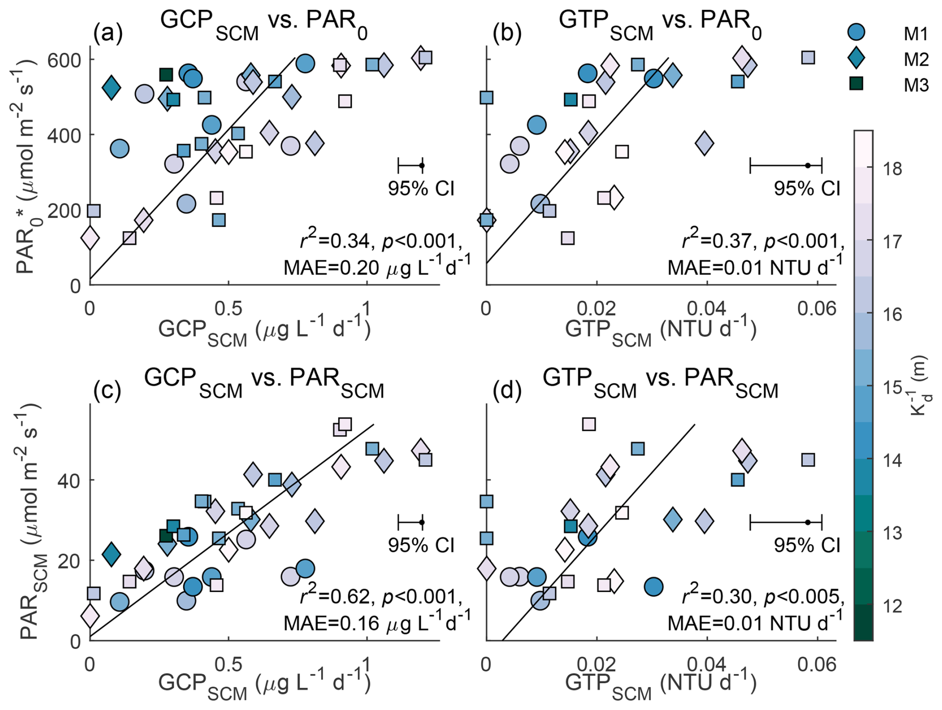
Figure 4 Light-limited productivity. Daily averaged PAR₀ (y axis, converted from shortwave radiation) vs. (a) GCP_SCM and (b) gross turbidity production (GTP_SCM) for all profilers and sample days with a good diel cycle fit (r²≥0.4), colored corresponding to the inverse diffuse attenuation ($K_{\mathrm{d}}^{-\mathrm{1}}$). (c, d) Similar to the above panel, but with PAR_SCM. We least-squares linear fit each panels gross production and light variable, labeling the resulting linear regression (black), r², p value, and mean absolute error (MAE).

We also note that due to the SCM depth being approximately 10 m deeper at M1 compared to the other profilers, PAR_SCM was lowest, on average, at this profiler. We can slightly improve the fit (MAE decreased by 12 %) of GCP_SCM to PAR_SCM (Fig. 4b) by accounting for phytoplankton light adaption by relating GCP_SCM to ${\mathrm{PAR}}_{\mathrm{SCM}}/\stackrel{\mathrm{‾}}{{\mathrm{PAR}}_{\mathrm{SCM}}}$ instead of PAR_SCM, where $\stackrel{\mathrm{‾}}{{\mathrm{PAR}}_{\mathrm{SCM}}}$ is the along-isopycnal average of the PAR_SCM at each profiler. This suggests phytoplankton were adapted to a lower irradiance (i.e., isolume) at M1 than the other profilers, but regardless, GCP_SCM similarly increased for larger PAR_SCM.

Despite the occasional non-algal sources of high turbidity, especially at M3, we estimated a good diel cycle fit (r²≥0.4) in turbidity for 28 d in total across the three profilers. The estimated gross turbidity production at the SCM (GTP_SCM) linearly varied with PAR at the surface and SCM, similar to GCP_SCM variability (Fig. 4b and d). This indicates the co-variability of ChlF_SCM and light availability is not limited to pigment concentration (e.g., photo-acclimation) but also corresponds to changes in biomass.

Our findings of light-limited ChlF could additionally be found by analyzing the instantaneous ChlF_SCM and depth-integrated ChlF, but the relationships were much weaker. We compared depth-integrated ChlF over the upper 80 m to depth-integrated PAR, and ChlF_SCM to PAR_SCM. Both linear regressions returned weak correlations (r²≤0.13) that remained significant (p<0.001, not shown). The instantaneous and depth-integrated ChlF was additionally influenced by ChlF loss and represents the accumulated biomass rather than just growth. Despite this, the strong influence of light availability on ChlF variability remained evident in both instantaneous ChlF_SCM and GCP_SCM.

3.3 Barrier layer stability

In the southern BoB, SCM productivity was linked to barrier layer thickness, defined as the depth-region between the mixed layer depth (MLD) base and the isothermal layer (ITL, Prasanth et al., 2023). Here, we define the ITL depth as the shallowest depth where the temperature was at least 1 °C cooler than the sea surface temperature (ΔT≤1 °C), and the MLD as the shallowest depth where the density increase from the surface value corresponds to a temperature decrease of 1 °C. The ITL was on-average within 1.5 m of the SCM depth at M3 and the barrier layer thickness was highly dependent on salinity variations (Fig. 5a–c).

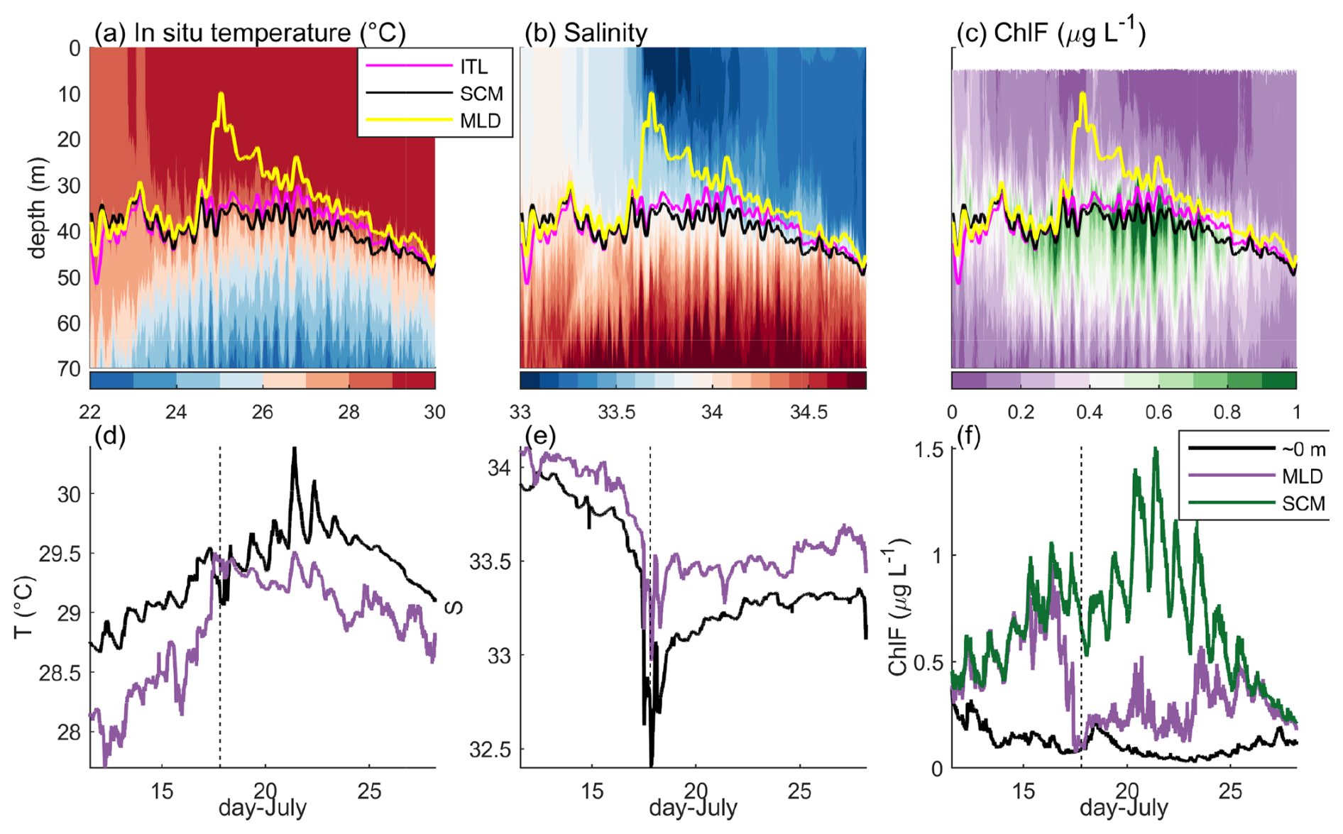
Figure 5 Barrier layer vs. the SCM. At M3, (a, d) in situ temperature, (b, e) salinity on the practical salinity scale, and (c, f) ChlF, over the upper 70 m (a–c) and at specific depths (d–f). (a–c) Depth of the isothermal layer (ITL, pink), SCM (black), and mixed layer depth (MLD, yellow). (d–f) Variability at near-surface (black), and mixed layer depth (purple). (f) Variability at the SCM (green).

While M3 was within the coastal plume (before 15 July), the MLD approximately equaled the SCM depth, which continued till 17 July (Fig. 5a and b). While within the plume, water temperature and salinity at the surface and MLD were different, indicating a very thin barrier layer was present, but ChlF was the same (Fig. 5d–f). A passing storm resulted in a shallow rain-layer forming around 17 July, the rapid shoaling of the MLD, diverging surface and MLD temperature and salinity (see Kerhalkar et al., 2025), and a rapid decrease in ChlF at the MLD base (Fig. 5). Over the remaining observation period, the MLD deepened until it reached the SCM around July 25. ChlF at the MLD and SCM then converged, and surface ChlF increased despite the transition to active monsoon conditions and decrease in light availability. The thick barrier layer that formed from the rain event should theoretically isolate upper ocean mixing from the SCM. The observed increase in ChlF_SCM and GCP_SCM from 18 July may therefore be due to both the sustained sunny break conditions and a decrease in SCM mixing from the barrier layer formation (Fig. 3d).

3.4 Regional and seasonal context

To determine whether our observations of co-varying PAR_SCM and GCP_SCM in the central Bay of Bengal were representative of the region and season, we analyzed the BGC-Argo subsurface ChlF, ERA5 estimated PAR and MODIS-Aqua diffuse attenuation climatology (see Sect. 2.4 and 2.5). To illustrate, we show one example of positively correlated PAR_SCM and ChlF_SCM over 12 months (WMO ID: 2902193; r²=0.58, p<0.001, and n=70; Fig. 6). At the seasonal time scale, trends in PAR_SCM were more similar to SCM depth than the incident surface PAR, where PAR exponentially decays with depth and so SCM depth can largely control PAR_SCM. In contrast, during the monsoon months of June to September, temporal variability was comparable between surface PAR and ChlF_SCM. This intraseasonal signal was sufficiently strong such that during the southwest monsoon period, surface PAR and subsurface ChlF (averaged over the upper 140 m) were significantly positively correlated (r²=0.26, p<0.01, and n=27), even without accounting for changes in SCM depth.

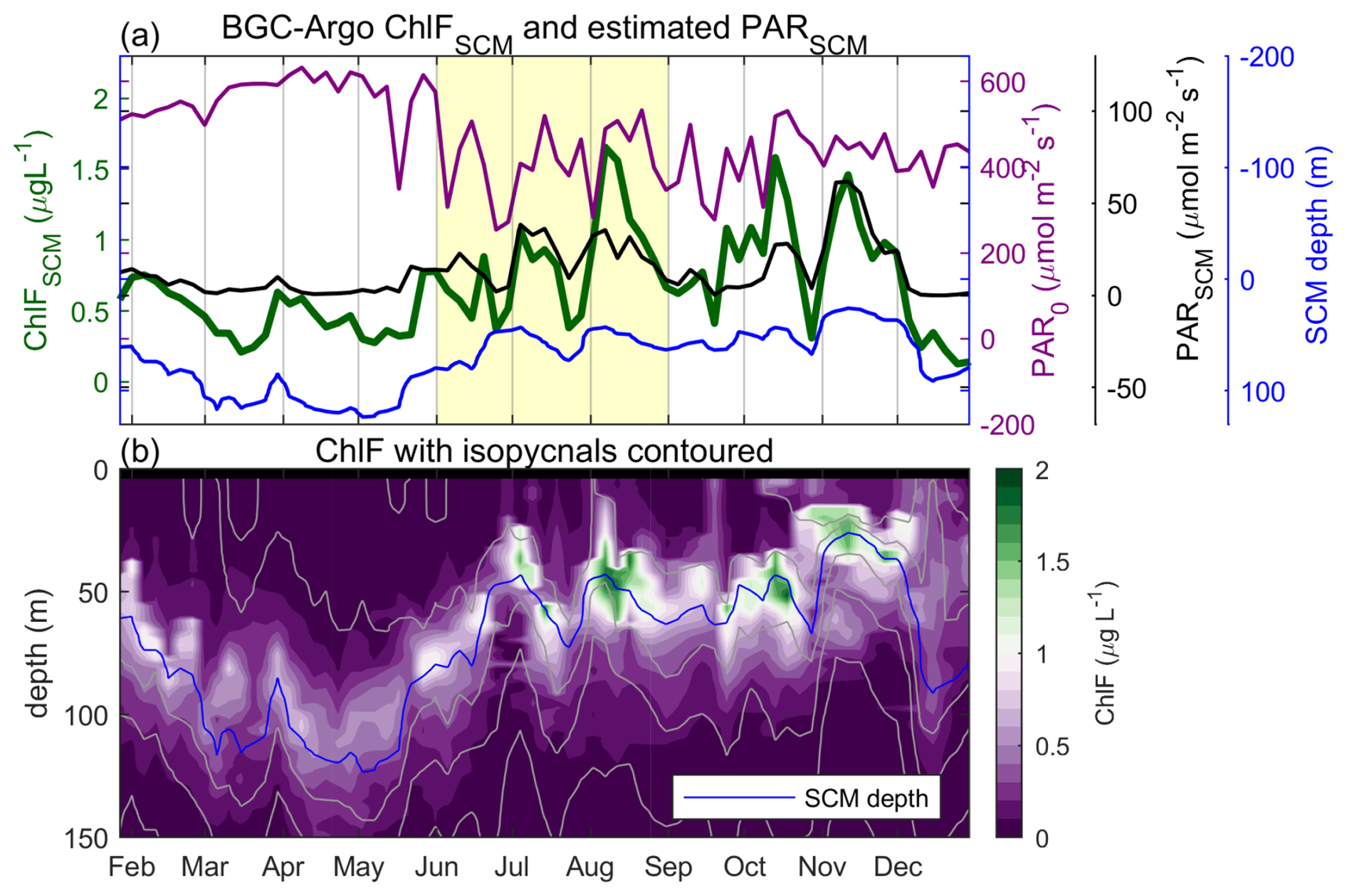
Figure 6 Co-varying light and ChlF from a 2016 BGC-Argo deployment (WMO ID: 2902193, Fig. 1a). ChlF concentrations (a) depth-averaged over the 20 m centered on the 1022 kg m⁻³ isopycnal we designate as the SCM (green, left y axis) and (b) contoured over depth. Also on panel (a), for each BGC-Argo profile we find the closest ERA5 surface PAR (purple, right y axis; Hersbach et al., 2018) and MODIS-Aqua 490 nm diffuse attenuation (Goddard Space Flight Center and Ocean Ecology Laboratory, 2018a), converted to a PAR equivalent (Morel et al., 2007), to estimate PAR_SCM (black, right y axis). Yellow shading in panel (a) indicates the southwest monsoon period. In panel (b), isopycnals are contoured in gray every 1 kg m⁻³, with the SCM plotted in blue.

The BGC-Argo float observed the largest change in ChlF_SCM during the southwest monsoon between the end of July and start of August. The minimum and maximum PAR_SCM around this time were on 23 July and 6 August, with observed ChlF_SCM on these days of 0.38 and 1.65 µg L⁻¹, respectively (Fig. 6). The time of observation will also impact ChlF_SCM in this region of strong diel cycles. We note the time of sampling of the minimum and maximum PAR_SCM was at 16:12 and 03:08 LT, respectively, where the DBASIS float observed daily maximum ChlF_SCM at 15:00 LT and minimum at 07:00 LT, on average (Fig. 3c). The over 300 % increase in ChlF_SCM observed by BGC-Argo was not only due to the transition from active to break monsoon conditions (Fig. 6), but also the shoaling of the SCM that further increased light availability.

If we contrast to the DBASIS platform observations, at M3 ChlF_SCM decreased from 0.96 to 0.58 µg L⁻¹ on 21 to 25 July, and at the same local time as the minimum and maximum BGC-Argo sample (Fig. 3c). This equates to a 40 % difference at M3, compared to the 77 % difference in the BGC-Argo float. We note the change in gross ChlF production at the SCM at the DBASIS platform was double the ChlF_SCM change, at an ≥80 % decrease, where this number is independent of sampling time (Fig. 3e). This may suggest changes in gross ChlF production due to intraseasonal oscillations at the BGC-Argo exceeded what we observed at M3, given variability in ChlF_SCM was larger at the BGC-Argo float than at M3.

4 Discussion

4.1 Primary productivity during the southwest monsoon

During the 2019 monsoon in the central Bay of Bengal and away from the coastal plume, ChlF and turbidity had a subsurface maximum, denoted the subsurface chlorophyll maximum (SCM, Fig. 2), and the SCM almost always coincided with the 1021.5 kg m⁻³ isopycnal. Both ChlF and turbidity also had a diel periodicity at the SCM, further suggesting that variations in ChlF at the SCM represent similar changes in biomass, as has been previously shown in the Indian Ocean waters (Cornec et al., 2021; Prasanth et al., 2023). The diel periodicity in ChlF has been observed elsewhere in the BoB (Lucas et al., 2016; Prasanth et al., 2023), and highlights a tight coupling between phytoplankton growth and loss in these oligotrophic waters. At the SCM, the gross production derived from both ChlF and turbidity varied with PAR_SCM (Fig. 4). Estimated gross ChlF production at the SCM (GCP_SCM) responded to variations in light from passing monsoon storms and changing ocean clarity (Fig. 4b and Supplement). GCP_SCM, estimated from the diel cycle in ChlF_SCM, linearly scaled with surface shortwave radiation at each DBASIS system, but the fit was sensitive to changing ocean color and turbidity. By accounting for variations in diffuse attenuation by linearly scaling GCP_SCM with PAR_SCM rather than PAR at the surface (PAR₀), we improved the linear fit (Fig. 4). We conclude we observed light limited SCM growth, contrary to prior studies showing the subtropical oligotrophic waters were typically nutrient limited (e.g., Mignot et al., 2014).

The estimated GCP_SCM rapidly decreased following the transition from sunny “break” to cloudy “active” monsoon conditions by ≥80 % in the northern BoB (Fig. 3d and e). This intraseasonal signal in ChlF gross production was also evident in BGC-Argo ChlF measurements from central BoB, with a similar difference in ChlF_SCM levels during the active vs. break periods as that observed by our measurements (e.g., 24 July to 8 August in Fig. 6a). Due to the southwest monsoon, surface PAR fluctuates on timescales of days to months over the entire bay (Gadgil et al., 2005; Mandke et al., 2020; Shroyer et al., 2021). Average surface PAR increased from 20 to 8° N, while the monthly standard deviation in surface PAR decreases from north to south (Fig. 7). This indicates that the southern BoB waters have higher and more consistent surface PAR, and towards the north, intraseasonal oscillations have a larger impact on surface PAR. We hence predict our observed ≥80 % difference in SCM productivity due to intraseasonal oscillations was representative of northern and perhaps central BoB variability during the southwest monsoon, confirmed by the BGC-Argo observations from central BoB (Fig. 6). From the surface PAR fluctuations, we expect weaker but still prevalent oscillations in productivity to occur in more southern waters.

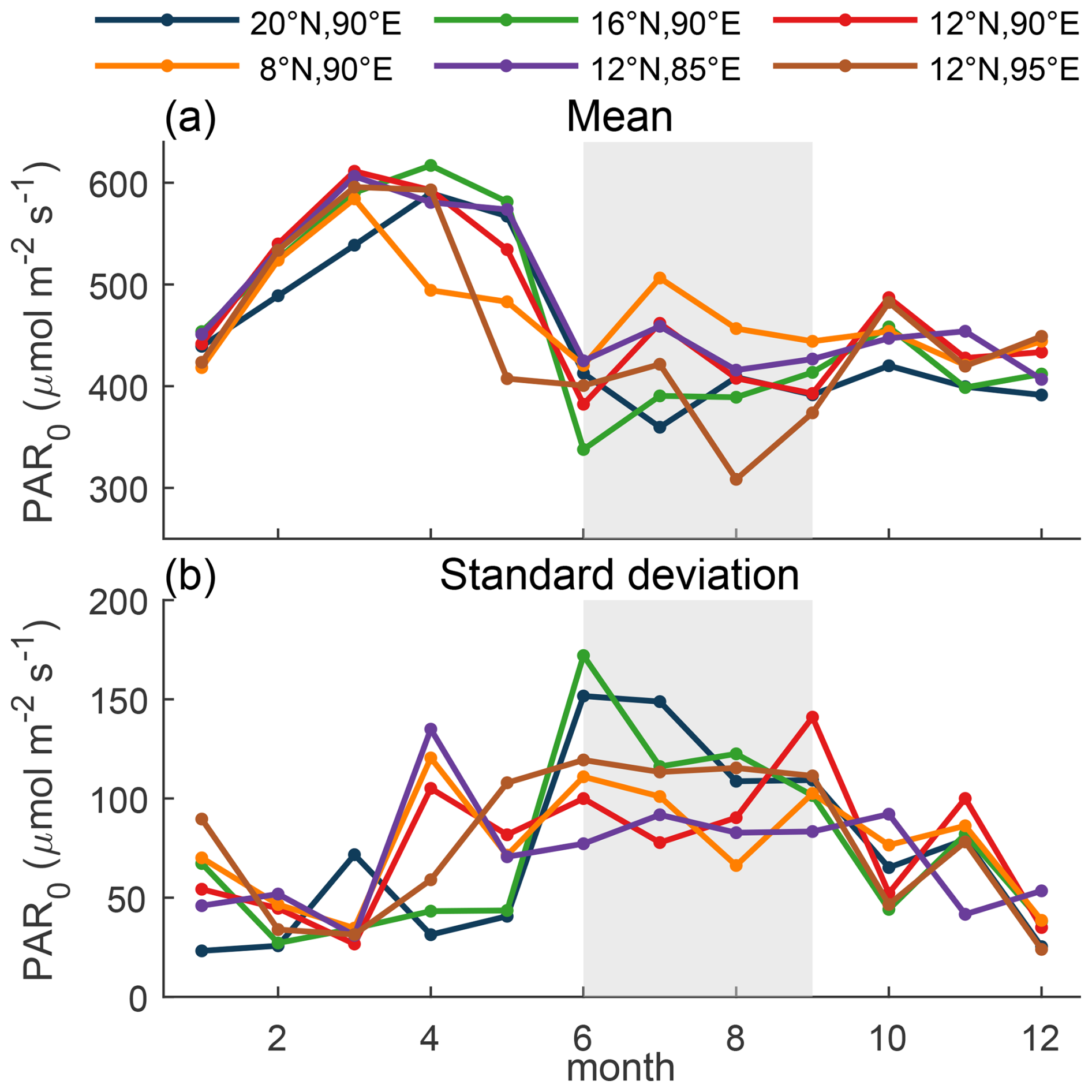
Figure 7 ERA5 derived monthly climatology (2012–2022) of surface PAR (PAR₀). ERA5 PAR₀ at fixed locations around the bay (color), (a) monthly averaged and (b) monthly standard deviation. Gray shading indicates the southwest summer monsoon period.

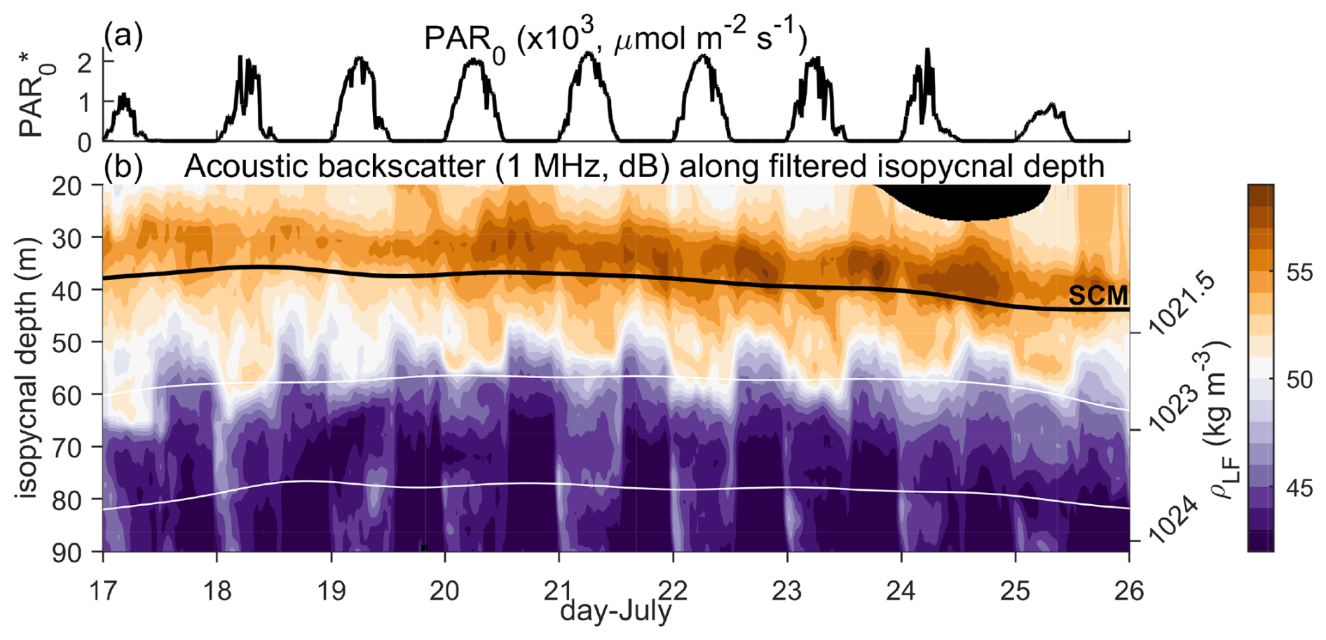
Figure 8 Diel vertical migration to the SCM. (a) PAR₀ (converted from shortwave radiation), and (b) on isopycnal acoustic backscatter at 1 MHz (depth as Fig. 3a).

Observations from the southern BoB have highlighted the importance of the barrier layer in supporting SCM productivity by impeding the mixing of the SCM into the mixed layer (Prasanth et al., 2023). Our observations deviated from the southern BoB observation but still confirmed the importance of the barrier layer. The formation of a shallow rain-layer rapidly shoaled the mixed layer, increasing the barrier layer thickness, and isolating the SCM from being eroded by upper ocean mixing (Fig. 5). Had the sunny break conditions not followed after a storm event, we expect observed intraseasonal oscillations in ChlF_SCM and GCP_SCM would have decreased. At M3, the erosion of the barrier layer co-occurred with minimum ChlF_SCM rather than when ChlF_SCM was enhanced, like observations by Prasanth et al. (2023). The erosion of the barrier hence had minimal impact on the already decreased SCM productivity, but likely contributed to the observed decrease in ChlF_SCM. We also note that at M3, the bulk of the SCM productivity was below the barrier layer, while Prasanth et al. (2023) observed enhanced ChlF within the barrier layer when it was present. As the SCM is typically located at the deepest depth where PAR is sufficient for growth and the shallowest depth where nutrients are available, our observations may suggest a relatively deeper nutricline than in the southern BoB. The barrier layer still separated the SCM from upper ocean mixing, and hence will influence SCM productivity, as found in the southern BoB (Prasanth et al., 2023).

Both the DBASIS and BGC-Argo observations indicate the intraseasonal variability in surface light project onto the SCM primary productivity. These observations suggest propagating coupled ocean-atmosphere intraseasonal weather patterns may leave a biological footprint of time- and space-variable primary productivity within the Bay of Bengal. Barrier layer formation is additionally impacted by intraseasonal oscillations (Thadathil et al., 2007; Girishkumar et al., 2011; Prasanth et al., 2023), and will impact ChlF vertical distributions (Prasanth et al., 2023) and hence SCM productivity. Other biogeochemical properties may also be dependent on intraseasonal weather patterns, since primary productivity modulates dissolved oxygen, particulate organic carbon, and dissolved inorganic carbon concentrations (Sarma et al., 2012). Similar patterns could also be evident in other tropical and subtropical oceans subject to intraseasonal atmospheric variability.

4.2 Higher trophic levels

Although we focus on the light limitation on primary productivity in this manuscript, grazing by higher trophic levels can also constrain phytoplankton variability. To provide some information on this component of the food web, we used acoustic backscatter measurements from 1 MHz Acoustic Doppler Current Profilers onboard the Wirewalkers (Fig. 8, Ohman et al., 2019). The backscatter measurements showed enhanced values at night in shallow waters with depths less than 50 m and density of 1022 kg m⁻³ or less (Fig. 8). Then during the day, backscatter measurements were enhanced in deeper waters at around 60 m depth. These observations are consistent with a shallow diel migration of zooplankton between around 60 m at daytime to near the SCM at nighttime. Although we do not have observations to confirm the size and species present, as highlighted in the “Introduction”, previous analysis with a 1 MHz acoustic backscatter confirms its sensitivity to smaller zooplankton species, including grazers (Lavery et al., 2007; Ohman et al., 2019; Gastauer et al., 2022). These smaller species tend to have slower and shallower vertical migrations than larger species (Gastauer et al., 2022), so the shallow diel migration in Fig. 8b is consistent with a small zooplankton species.

The acoustic backscatter strength near the SCM increased over time and reached a maximum on 24 July (Fig. 8b). During this period of increasing acoustic backscatter, the rate of ChlF_SCM loss began to exceed that of GCP_SCM (Fig. 3d), leading to a decrease in Chl_SCM from 21 July. This suggests that grazing could have contributed to the increased loss rate and might provide a link between intraseasonal variability in primary production and higher trophic levels. Prasanth et al. (2023) highlighted that a better understanding of barrier layer formation under variable phytoplankton growth rates and zooplankton grazing is required. Here, we reveal important linkages between these processes and additionally highlight the importance of the intraseasonal oscillations in imparting periodicity to phytoplankton growth at the SCM.

5 Conclusions

The coupled bio-optical and physical observations collected from the DBASIS drifting buoy-profiler systems allowed concurrent measurements of the subsurface irradiance and the diel cycles of subsurface chlorophyll fluorescence during the southwest monsoon (Fig. 3a). These observations showed that changes in subsurface irradiance in the northern Bay of Bengal were coupled with intraseasonal variability in monsoon weather and spatial variability in the turbidity of surface waters, and led to major changes in subsurface primary productivity.

Coupled ocean-atmosphere global forecasting models are challenged to accurately represent intraseasonal variability in the tropical and subtropical ocean. Here we have shown that intraseasonal variability extends to the subsurface biogeochemical properties of the Northern Indian Ocean. Representing this variability correctly in climate predictions is necessary to reduce forecast uncertainty since it impacts both the ocean carbon system and the optical characteristics of the upper ocean, which modulate ocean heat content. Continued advances in autonomous measurement techniques, and widespread deployment of those platforms, is necessary to improve our understanding of the contribution of intraseasonal biogeochemical variability to the ocean ecosystem.