Internal tides on the Al-Batinah shelf: evolution, structure and predictability

Internal tides are a key mechanism of energy transfer on continental shelves. We present observations of internal tides on the northern Oman shelf based on moored temperature and velocity records collected during 2021–2022. The regional shelf exhibits strong shallow summer stratification ($N_{\mathrm{peak}}^{\mathrm{2}}\sim {\mathrm{10}}^{-\mathrm{2}}{\mathrm{s}}^{-\mathrm{2}}$), supporting shoreward-propagating internal tides with pronounced fortnightly modulation in amplitude and energy fluxes. Despite semidiurnal dominance in barotropic forcing, the internal tides appear predominantly in the diurnal band. During summer, the incoming internal tide energy flux at our mooring on the central shelf (23 m depth, 10 km from shore), ranges around $F_{\mathrm{E}}^{\mathrm{in}}\sim \mathrm{5}$–15 W m⁻¹ and we estimate that the onset of main internal-tide dissipation occurs further inshore over the shallow inner shelf. As the thermocline deepens in fall, the onset of the saturation zone migrates seaward from its summer location to reach our central-shelf mooring by early October. There, waveform structures undergo seasonal transition from quasi-linear depression waves in summer to increasingly nonlinear features in fall, including steepening, asymmetry, polarity reversal and a shift toward first-mode dominance . In October $F_{\mathrm{E}}^{\mathrm{in}}$ increases to ∼ 30 W m⁻¹ primarily driven by the increasing nonlinearity as the internal tides reach their finite-depth shoaling regime over the central shelf. Cross-shelf coherence and phase-speed estimates also confirm that the observed internal tides maintain spatial coherence from the shelf edge inshore beyond the typical internal surf zone. Skill scores indicate that the predictability of the local internal tides decreases by 50 % after around 18 d, which is comparable to high-predictability sites globally. Inshore-directed energy flux, diurnal dominance and multi day phase lags to barotropic forcing still indicate remote generation. For the local barotropic tidal currents, variability in bulk KE and predictability-scores suggest seasonal modulation by the internal tides.

1 Introduction

Internal tides (ITs) are internal gravity waves generated by the interaction of barotropic tidal currents with topography in a stratified ocean (Vlasenko et al., 2005). These waves can propagate long distances, transferring energy from generation sites into the open ocean and onto continental shelves (Garrett and Kunze, 2007). As ITs shoal onto continental shelves, they undergo transformation through nonlinear steepening, dispersion, modal scattering, and dissipation (Kelly and Nash, 2010; Lauton et al., 2021). When remotely generated low-mode tides enter the shelf they often evolve into incoherent bores and boluses nearshore, driving turbulence and cross-shelf transport (Walter et al., 2014). Most energy dissipates before reaching shallow depths, with turbulent dissipation matching the flux divergence (Becherer et al., 2021a, b). Shoaling dynamics vary regionally with stratification, slope, and background currents (Masunaga et al., 2024), and energy partitioning among reflection, scattering, and transmission is spatially variable (Inall et al., 2011; Siyanbola et al., 2024). Their propagation is modulated by mesoscale variability and evolving stratification, resulting in both coherent and incoherent components (Kelly et al., 2015; Rayson et al., 2021). While harmonic and response-based models can predict some aspects – especially the coherent fraction – remote forcing and nonlinear interactions contribute to substantial unpredictability (Nash et al., 2012).

The Gulf of Oman (GoO, also known as the Sea of Oman) connects the Arabian Sea and Persian Gulf. The Al-Batinah shelf along northern Oman (between Sohar and Barka) is relatively shallow (∼ 30 m) and wide (∼20 km) compared to steeper margins elsewhere within the GoO. Regional circulation and water mass structure have been described by Johns et al. (1999) and Pous et al. (2004), with later studies expanding on mesoscale eddies (L'Hégaret et al., 2013, 2016), the role of Persian Gulf Water (Font et al., 2024; Queste et al., 2018), and monsoon-driven variability (DiMarco et al., 2023). Seasonal SST patterns and the influence of the summer monsoon on the Al-Batinah shelf are documented by Al-Hashmi et al. (2019) and DiBattista et al. (2022), while regional warming and stratification trends have been noted by Bordbar et al. (2024) and Piontkovski and Chiffings (2014). The vertical structure over the slope of the local shelf has been studied using gliders showing a shallow mixed layer above a sharp thermocline (TC) in summer, with the TC retreating offshore by November and a new mixed layer reestablishing over winter mode water by April (Font et al., 2022, 2024). Claereboudt (2018) and Chitrakar et al. (2020) provide the few available in situ vertical profiles from the northern Omani shelf, showing strong summer stratification and intermittent disturbances. Coles (1997), the earliest local dataset, reported temperature oscillations at sub-diurnal (tidal) frequencies from bottom-mounted thermistors near Fahal Island.

Regional observations of internal waves and tides in the GoO remain sparse. At the Strait of Hormuz, Pous et al. (2004) identified internal wave signatures linked to tidal intensification near the pycnocline. Small and Martin (2002) used SAR imagery and modeling to reveal nonlinear IT packets propagating onto the western shelf. Subeesh et al. (2025) documented seasonally modulated ITs in the western Strait of Hormuz, with enhanced generation during summer. Koohestani et al. (2023) mapped solitary wave hotspots across the basin, linking them among others to barotropic tidal forcing. Despite these advances, the generation, propagation, and impacts of ITs across much of the GoO remain poorly understood, limiting our ability to assess their broader ecological and biogeochemical significance.

Internal tides may have important regional implications. They can enhance vertical mixing and transport low-oxygen water from regional oxygen minimum zones onto the shelf, contributing to seasonal hypoxia, harmful algal blooms, and fish kill events. Additionally, they may provide thermal relief to coral reefs by delivering cooler subsurface waters, thereby protecting corals from heat stress (Storlazzi et al., 2020). Understanding these processes is crucial for predicting ecosystem responses to climate change, managing coastal resources, and improving forecasts of biogeochemical variability linked to internal wave-driven cross-shelf exchange.

Here, we present new observations of internal tides on the Al-Batinah Shelf based on moored velocity and temperature records. The study aims to characterize their temporal variability and vertical structure, quantify energy fluxes and waveform evolution, and assess spatial coherence and predictability in comparison to global observations. These results provide the first detailed view of internal tides in this region and their potential role in local shelf dynamics.

2 Methods

2.1 Study area

The Al-Batinah shelf lies in the southwest of the GoO in front of the Oman coast between Sohar and Seeb. The average shelf width to the shelf break at 100 m is around 25 km, after which there is a short steep slope followed by a more gradual descent from about 250 m to 3 km (Fig. 1). Within the study area between Al Kaburah and the Sawadi headland, isobaths shallower than 200 m are approximately oriented along the 285–105° (WNW–ESE) axis. The study area lies at a latitude of around 24° with an inertial period of ∼ 29.5 h (f≈0.81 cpd) and is thus subcritical for the diurnal tidal band. The critical latitudes of the main diurnal harmonics are 30° for K₁ and 27.6° for O₁. The locations of the two mooring stations at Raqqat As Suwayq (RAS) and Inshore Suwayq (ISQ) are indicated on the map in Fig. 1.

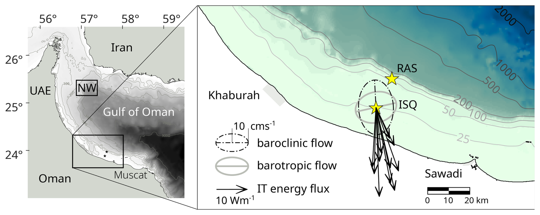
Figure 1 Map of study area and field sampling locations. Bathymetry is from GEBCO (2024). The locations of the on-shelf moorings are shown by yellow markers. Vectors at ISQ represent the energy flux of the diurnal ITs from 15 August to 10 October. Baroclinic and barotropic flow components are indicated by best-fit ellipses.

2.2 Data and basic diagnostics

On the crest of the small seamount Raqqat As-Suwayq (RAS, Fig. 1), near the shelf edge, temperature at approximately 18 m depth and currents were recorded with an Acoustic Doppler Current Profiler (ADCP) over a 22-month period from January 2021 to October 2022. Depth-averaged on-shelf stratification was derived by comparing temperatures recorded by near-bottom sensors at RAS with satellite-derived sea surface temperature (SST). To resolve the vertical thermal structure of the oscillations observed in the bottom temperature, a full-depth mooring was deployed at ISQ in 23 m water depth (Fig. 1).

At the ISQ mooring, current profiles were recorded at 5 min intervals using a bottom-mounted, upward-looking ADCP (AWAC 600 kHz, with 0.5 m bin size) for approximately four months in winter 2021/2022 (October–January) and three months in summer 2022 (mid July–mid October). Concurrently, during the summer deployment, a time series of the temperature profiles was recorded at the same station using a vertical thermistor chain of HOBO loggers with ∼ 2 m vertical and 15 min temporal resolution. High sensor drift in conductivity probes, primarily due to strong biofouling on the shallow shelf, prevented reliable long-term salinity measurements at similar vertical and temporal resolution. Salinity data are therefore limited to discrete CTD casts. For calculations requiring density (e.g., N² or potential energy anomaly), a constant salinity value was used. This value represents the mean salinity from all available CTD casts near the ISQ mooring location during four summer periods between 2021 and 2024 (cf. Fig. 2).

Seawater potential density ρ_θ and buoyancy frequency $N^{\mathrm{2}}=-\frac{g}{{\mathit{\rho }}_{\mathrm{0}}}\frac{\mathrm{d}{\mathit{\rho }}_{\mathit{\theta }}}{\mathrm{d}z}$ were calculated using the GSW Oceanographic Toolbox according to TEOS-10 (McDougall and Barker, 2011) and we also calculate vertical shear $S^{\mathrm{2}}={\left(\mathrm{d}\mathit{u}/\mathrm{d}z\right)}^{\mathrm{2}}$ and Richardson number $Ri=N^{\mathrm{2}}/S^{\mathrm{2}}$. To define the depth of the mixed layer we use conventional definitions and define thermocline elevation z_TC as the depth at which the temperature θ falls below a certain threshold relative to the surface temperature: $z_{\mathrm{TC}}\left(t\right):\mathit{\theta }(z,t)={\mathit{\theta }}_{\mathrm{surf}}\left(t\right)-\mathrm{\Delta }\mathit{\theta }$. Surface temperature here refers to the uppermost temperature from the mooring, which is ∼3 m below the actual surface (Fig. 3b) but practically always within the upper (well) mixed layer. The value of Δθ is determined by fitting the variation of z_TC over the record period to match the variation of the vertical level of the upper N² peak. For the data from ISQ Δθ=2 °C which is larger than commonly used threshold values around 1 °C.

Information on the barotropic tide was derived from the pressure sensor of the ADCP as well as from the TPXO regional tidal model solution for the Persian Gulf/Gulf of Oman (Egbert and Erofeeva, 2002). Satellite-derived SST was obtained from the OSTIA dataset (Good et al., 2020).

2.3 Background conditions and tidal-band decomposition

To estimate background conditions, except for vertical N² profiles, we apply a low-pass filter in the frequency domain with a tapered cutoff at 50 h and denote background (low-pass filtered) quantities with a tilde. To determine background stratification (N² profiles) we do not average the available temperature profiles over a tidal cycle as this would diffuse z_TC over a wider depth range, thus reducing the N² peak. We rather consider background conditions at the times when the instantaneous z_TC crosses the low-pass filtered z_TC (see Sect. 3.1).

To further isolate variability in the diurnal (D-band) and semidiurnal (SD-band) frequency bands, we apply wavelet-based decomposition to the baroclinic signals using the maximal overlap discrete wavelet transform (MODWT) with a Symmlet-4 wavelet. Reconstruction within the 8–16 h (SD-band) and 16–32 h (D-band) bands is used to extract time-localized tidal variability. Note that the D-band also contains energy near the local inertial frequency (∼ 28 h period).

The barotropic tidal transport from the TPXO model is decomposed as the sum of predicted contributions from tidal constituents in each band: D-band ($K_{\mathrm{1}},O_{\mathrm{1}},P_{\mathrm{1}},Q_{\mathrm{1}}$) and SD-band ($M_{\mathrm{2}},S_{\mathrm{2}},N_{\mathrm{2}},K_{\mathrm{2}}$). Amplitude spectra are computed using standard FFT-based methods to characterize the stationary (phase-locked) components of the signal, and tidal harmonic analysis is performed using the UTide package (Codiga, 2011).

2.4 Properties of Internal Tides

Individual internal tides are defined between upward crossings of the instantaneous z_TC through the low-pass filtered z_TC. Individual tides were identified from the original signal as well as for the decomposed D- and SD-bands. All individual tides identified by the automatic zero-crossing detection were visually verified. Periods where individual ITs could not be clearly identified were omitted from further analysis and appear as gaps in the respective figures. Variables like the root mean square of the thermocline displacement ξ_rms, phase speed c_p, wavelength L, energy flux F_E and wave asymmetry/polarity are determined by integrating over each of the individual ITs.

As ITs shoal on the inner shelf, they steepen and become increasingly nonlinear, ultimately forming sharp bore fronts (McSweeney et al., 2020; Becherer et al., 2021a). Wave asymmetry is quantified by the skewness of the temporal gradient $\mathrm{d}\mathit{\xi }/\mathrm{d}t$, computed within each wave. Positive skewness indicates a steeper leading edge relative to the trailing face. The polarity of an internal wave distinguishes between waves of depression and waves of elevation. Although this concept is more commonly applied to internal solitary waves (ISWs), we also assess a simplified polarity metric defined as the ratio of the maximum upward to downward displacement.

2.5 Spatial coherence

To assess the relationship between the recorded baroclinic signals at ISQ and the local surface tide, we analyze the barotropic tidal transport from the TPXO model over the local shelf slope. We examine the phase relationship between the fortnightly amplitude modulation of the barotropic transport and that of the internal tides. This analysis is performed in both the D- and SD-bands by extracting the amplitude envelope using the Hilbert transform of the complex velocity time series (u+iv).

Time lags between signals at RAS and ISQ are determined from three months of temperature records at both stations at 18 m depth. Tidal events within the extended tidal band (6–36 h) are isolated, and time lags are estimated by cross-correlating each ISQ event with the RAS record. Both signals are locally normalized prior to correlation. Phase speeds are then computed by projecting the RAS–ISQ separation onto the direction of the corresponding IT energy flux.

Another simple phase speed estimation of long internal waves in a two-layer, non-rotating, inviscid fluid system is given by the classical shallow-water approximation, which depends on the density contrast between layers, gravitational acceleration, and the harmonic mean of the layer depths: $c_{\mathrm{p}}=\sqrt{g^{\prime }\frac{h_{\mathrm{1}}{h}_{\mathrm{2}}}{h_{\mathrm{1}}+h_{\mathrm{2}}}}$, where $g^{\prime }=g\mathrm{\Delta }\mathit{\rho }/\mathit{\rho }$ and Δρ is the density difference between the two layers, ρ is a reference density (typically the lower layer), g is the gravitational acceleration, and h₁, h₂ are the layer thicknesses. Phase speeds determined via these two methods are compared to estimates obtained from modal analysis.

2.6 Internal tide energy flux, PEA and KE

We decompose flow and pressure and determine internal wave energy flux following Kunze et al. (2002) and Kelly and Nash (2010). The baroclinic component of the flow u^′ is obtained by ${\mathit{u}}^{\mathbf{\prime }}(z,t)=\mathit{u}(z,t)-\stackrel{\mathrm{̃}}{\mathit{u}}(z,t)-{\mathit{u}}_{\mathrm{0}}\left(t\right)$ in which u is the instantaneous (measured) current, $\stackrel{\mathrm{̃}}{\mathit{u}}$ is the low-pass filtered flow and u₀ is determined via the baroclinicity condition $\frac{\mathrm{1}}{H}{\int }_{-H}^{\mathrm{0}}{\mathit{u}}^{\mathbf{\prime }}(z,t)\mathrm{d}z=\mathrm{0}$ which requires that u^′ vanishes when integrated over the water column (e.g. Kunze et al., 2002). The removal of the low-frequency component $\stackrel{\mathrm{̃}}{\mathit{u}}$ isolates the internal wave motions, particularly those at super-inertial frequencies (e.g., D- and SD-bands). Because the background conditions vary gradually and significantly over the long record, all-time means are unsuitable here. Removal of the low-frequency component is furthermore important since the background flow is also baroclinic.

The energy flux of the internal waves is calculated as $F_{\mathrm{E}}=〈{\mathit{u}}^{\mathbf{\prime }}{p}^{\prime }〉$. The brackets 〈⋅〉 denote a time average, typically over a certain fixed window or over one phase of the internal tide. The pressure perturbation p^′ due to the internal waves is obtained by vertical integration of the density anomaly $p^{\prime }(z,t)={\int }_z^{\mathrm{0}}{\mathit{\rho }}^{\prime }(z^{\prime },t)g\mathrm{d}{z}^{\prime }+p_{\mathrm{surf}}\left(t\right)$. The surface pressure p_surf results again from applying the baroclinicity condition (i.e. the pressure perturbation must vanish when integrated over the depth). The density anomaly ${\mathit{\rho }}^{\prime }(z,t)$ is estimated from the vertical displacement of isotherms ξ(z,t) using the linearized equation of state under the Boussinesq approximation: ${\mathit{\rho }}^{\prime }(z,t)=\left(\stackrel{\mathrm{̃}}{\mathit{\rho }}\right(z)/g)N^{\mathrm{2}}\left(z\right)\mathit{\xi }(z,t)$. We use the displacement of isotherms rather than isopycnals due to the lack of high-resolution salinity data as described above. Isotherm displacement is calculated as: $\mathit{\xi }(z,t)=-{\mathit{\theta }}^{\prime }(z,t)\left(\partial z/\partial \stackrel{\mathrm{̃}}{\mathit{\theta }}\right)$ where θ^′ and $\stackrel{\mathrm{̃}}{\mathit{\theta }}$ denote baroclinic and low-pass filtered temperature respectively.

We use Potential Energy Anomaly (PEA) as a measure for the overall strength of the water column stratification. We use the definition of PEA that was first proposed by Simpson (1981):

$$\begin{array}{}\text{(1)}& \mathrm{PEA}\left(t\right)={\displaystyle \frac{\mathrm{1}}{D}}\underset{-H}{\overset{\mathit{\eta }}{\int }}\left(\stackrel{\mathrm{‾}}{\mathit{\rho }}\right(t)-\mathit{\rho }(z,t\left)\right)gz\mathrm{d}z\end{array}$$

where D is the total water depth from the sea floor at −H to the free surface η and $\stackrel{\mathrm{‾}}{\mathit{\rho }}$ is the depth-averaged density.

PEA quantifies the energy required to fully mix a vertically stratified water column to a state of uniform density. In this study, we focus on the low-frequency variability of PEA and therefore neglect the effects of tidal deformation of the water column, which can be significant when tidal amplitude is comparable to the water column thickness (Hamada and Kim, 2021). We compute PEA at the full temporal resolution of our dataset and subsequently derive daily (Fig. 3b) and IT phase-averaged values (Fig. 5). Kinetic energy KE $=\frac{\mathrm{1}}{\mathrm{2}}{\mathit{\rho }}_{\mathrm{0}}〈\stackrel{\mathrm{‾}}{(u^{\mathrm{2}}+v^{\mathrm{2}})}〉$ is computed for unfiltered flow, band-pass filtered components, and for barotropic and baroclinic currents. Bulk values are obtained by averaging over depth ($\stackrel{\mathrm{‾}}{\cdot }$) and over specified periods (〈⋅〉) for summer and winter (cf. Fig. 2).

2.7 Dynamic modes

We determine vertical dynamic modes by solving the vertical structure eigenvalue problem. The governing equation for vertical displacement or vertical velocity amplitude is derived from the linearized, hydrostatic, Boussinesq primitive equations (Cushman-Roisin and Beckers, 2011), resulting in a Sturm–Liouville eigenvalue problem of the form:

$$\begin{array}{}\text{(2)}& {\displaystyle \frac{{\mathrm{d}}^{\mathrm{2}}}{\mathrm{d}{z}^{\mathrm{2}}}}\mathrm{\Phi }\left(z\right)+{\displaystyle \frac{N^{\mathrm{2}}\left(z\right)}{c_{\mathrm{e}}^{\mathrm{2}}}}\mathrm{\Phi }\left(z\right)=\mathrm{0}\end{array}$$

which we solve for the boundary conditions $\mathrm{\Phi }(-H)=\mathrm{\Phi }\left(\mathrm{0}\right)=\mathrm{0}$. To quantify modal energy partitioning, we project the observed baroclinic velocity fields onto the horizontal modes $p\left(z\right)\propto \mathrm{d}\mathrm{\Phi }\left(z\right)/\mathrm{d}z$ which are L² normalized such that ${\int }_{-H}^{\mathrm{0}}{p}^{\mathrm{2}}\left(z\right)\mathrm{d}z=\mathrm{1}$. Modal amplitudes are then computed as:

$$\begin{array}{}\text{(3)}& A_n\left(t\right)=\underset{-H}{\overset{\mathrm{0}}{\int }}{\mathit{u}}^{\mathbf{\prime }}(z,t)p_n(z,t)\mathrm{d}z\end{array}$$

where u^′ is the observed baroclinic cross-shelf current. The normalization ensures that $A_n^{\mathrm{2}}$ is proportional to the energy content in mode n, enabling consistent comparison of relative energy between modes and across time segments. The vertical modes shown in Fig. 4 are scaled with these modal amplitudes. From the eigenspeeds c_e we determine phase speed under the influence of rotation via the dispersion relation as in Rainville and Pinkel (2006):

$$\begin{array}{}\text{(4)}& c_{\mathrm{p}}\equiv {\displaystyle \frac{\mathit{\omega }}{({\mathit{\omega }}^{\mathrm{2}}-f^{\mathrm{2}}{)}^{\frac{\mathrm{1}}{\mathrm{2}}}}}{c}_{\mathrm{e}}\end{array}$$

2.8 Predictability

In order to determine the predictability of the internal tides we apply the methods following Nash et al. (2012) (based on the skill score by Murphy, 1988). Predictability is quantified through the analysis of a skill score (SS, Eq. 5) that measures how much of the variance of the signal (Ψ, currents or temperature) is captured by harmonic analysis in moving windows H_T with different window size T. We perform tidal harmonic analysis with the UTide package (Codiga, 2011).

$$\begin{array}{}\text{(5)}& {\mathrm{SS}}_T=\mathrm{100}\mathit{\%}\times \left[\mathrm{1}-{\displaystyle \frac{〈(\mathrm{\Psi }-H_T(\mathrm{\Psi }){)}^{\mathrm{2}}〉}{〈{\mathrm{\Psi }}^{\mathrm{2}}〉}}\right]\end{array}$$

To enable direct comparison with the global predictability estimates reported by Nash et al. (2012), we applied harmonic fits using the same six tidal constituents ($M_{\mathrm{2}},S_{\mathrm{2}},N_{\mathrm{2}},K_{\mathrm{1}},O_{\mathrm{1}}\mathrm{and}{J}_{\mathrm{1}}$), even for short time windows (as short as 5 d). While individual constituents are not spectrally resolvable over such durations, their combined fit offers a consistent measure of variance within the broadened tidal band. A predictability timescale T_50 % is defined as the window length at which the variance explained by the harmonic fit declines to halfway between its maximum (at short durations) and its asymptotic long-term value, approximated by the fit at T=180 d. This metric reflects the temporal coherence of the internal tide and captures the rate at which phase and amplitude relationships decorrelate under evolving background conditions. While the two summer temperature records at RAS span 180 d, the ISQ records are shorter (October 2021–January 2022 (winter), and July–October 2022 (summer)). For these shorter records, we fit a power-law decay of the form SS$\left(T\right)=a/T^b$ to estimate the Skill Score at 180 d, acknowledging the associated limitations.

3 Results and Discussion

The 22-month temperature record from the shelf-break mooring at RAS (Fig. 2a) shows that during winter (December–March), the temperature at 18 m depth approximately matches the remotely sensed daily averages of foundation sea surface temperature (SST), indicating fully mixed conditions and small variations in the tidal band. The lowest temperatures, around 23 °C, occur in February. Restratification begins in March, marked by a simultaneous increase in both SST and bottom temperature, accompanied by a growing divergence between them. During summer, high surface temperatures exceeding 32 °C appear in early June in both years. Stratification then breaks down beginning in October, as SST decreases while bottom temperature rises, leading to temperature homogenization by December.

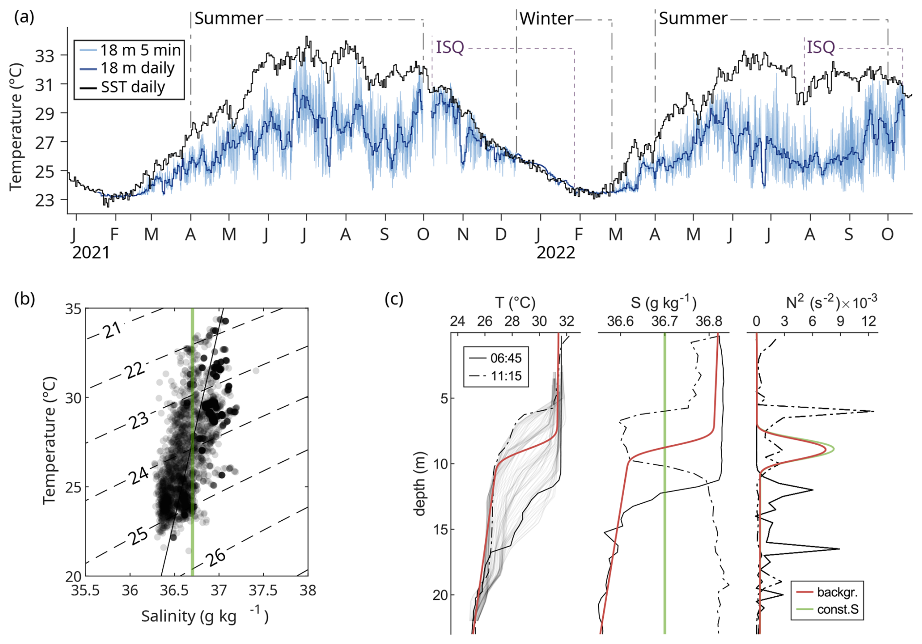
Figure 2 Temperature, salinity, and stratification in the study area. (a) Twenty-two-month temperature record from the RAS mooring at 18 m depth (5 min and daily averages) and satellite-derived daily SST. (b) T–S diagram of all available on-shelf CTD casts from four summer periods (2021–2024) near the ISQ station. Contour lines indicate isopycnals; the green vertical line marks the approximate average salinity used in this study. (c) Vertical profiles of temperature (T), salinity (S), and buoyancy frequency (N²). Solid and dashed black lines represent CTD casts taken 4.5 h apart during the flood phase of the internal tide on 25 August 2022. Thin grey lines in the temperature panel show profiles from the vertical thermistor chain. Green lines indicate constant salinity; the red line shows background stratification.

The main differences between the two recorded years stem from interannual variability in the local influence of the Southwest Monsoon over the Arabian Sea between June and September. In 2022, persistent easterly winds from June to October sustained offshore surface transport, resulting in prolonged low-frequency upwelling. The lowest water temperatures occurred in early August, followed by a gradual warming as the winds weakened. Similar dynamics have been described by DiMarco et al. (2023) for the shelf off Sohar, 150 km to the northwest.

Shorter, more intense summer upwelling events occasionally reached the surface (e.g., in July 2021), although a vertical temperature gradient was typically retained. Because the in situ temperature record at RAS generally reflects conditions below the shallow thermocline, the temperature difference between surface and bottom serves as an indicator of upper-water-column stratification strength. Between the two years, summer stratification was stronger in 2022, when the daily averaged vertical temperature difference from the surface to 18 m ranged between 4–7 °C, peaking at 9.3 °C on 25 June 2022. Daily variations in bottom temperature at RAS during summer averaged around 4 °C, with maxima up to 8 °C. A spectral analysis of the RAS record is presented in Sect. 3.4.

From CTD casts, we frequently observe a salinity inversion in summer, with higher salinity above z_TC. Figure 2b shows data from 47 CTD casts near the ISQ mooring location during four summer periods between 2021 and 2024. The salinity inversion is reflected in the positive slope of the linear fit in the T–S diagram and is attributed to surface evaporation combined with limited vertical mixing across the thermocline. This inversion reduces the vertical density gradient, thereby weakening the actual pycnocline (N² peak). Consequently, variables derived from stratification, such as IT energy flux or potential energy anomaly (PEA) estimates, may be slightly overestimated if calculated solely from thermal stratification. We assess this effect to be small (see below). Despite the salinity inversion, salinity variability is relatively low compared with temperature, both vertically and spatially across the shelf and over the years surveyed. To calculate density in the absence of high-resolution salinity measurements for the ISQ summer data, we therefore use an average salinity from all CTD casts. The green vertical line in the T–S diagram indicates this average salinity value.

Two CTD casts at the ISQ station on 25 August 2022 (Fig. 2c) illustrate short-term variability during rising internal tides. Offshore bottom flow produced a temporary three-layer structure, with a 6 m uplift of the thermocline and corresponding halocline displacement (Fig. 4). Salinity increased in the lower layer during the flood phase, likely reflecting either intrusion of Persian Gulf Water or subduction and offshore transport of high-salinity inner-shelf water by cascading, downwelling, or internal tides (Shapiro et al., 2003). A shallow diurnal warm layer of 0.8 °C can be seen in the upper 1.4 m of the second profile accompanied by a small rise in surface salinity. Only two salinity profiles are available for this day. We retain the upper halocline gradient as background stratification and approximate the deeper profile from the earlier cast, excluding the bottom anomaly. The resulting N² profiles show that including the observed salinity inversion reduces the stratification peak by <5 % relative to constant salinity. This small effect supports the use of temperature-based density estimates for the 11-week energy flux calculations.

3.1 Evolution of Internal Tides

Figure 3 presents the two main observed variables (temperature and horizontal currents, Fig. 3b–c) from the ISQ mooring, together with derived properties of the internal tides. The dataset spans 11 weeks towards the end of summer, covering both summer conditions and the autumnal transition of stratification. For a short period at the beginning of the record, stratification is weak due to a preceding wind-driven upwelling event (not shown). During the first week of August, stratification is re-established, with a shallow z_TC at approximately 8 m below the surface (15 m above the bottom), and surface temperatures exceeding 32 °C (Fig. 3b).

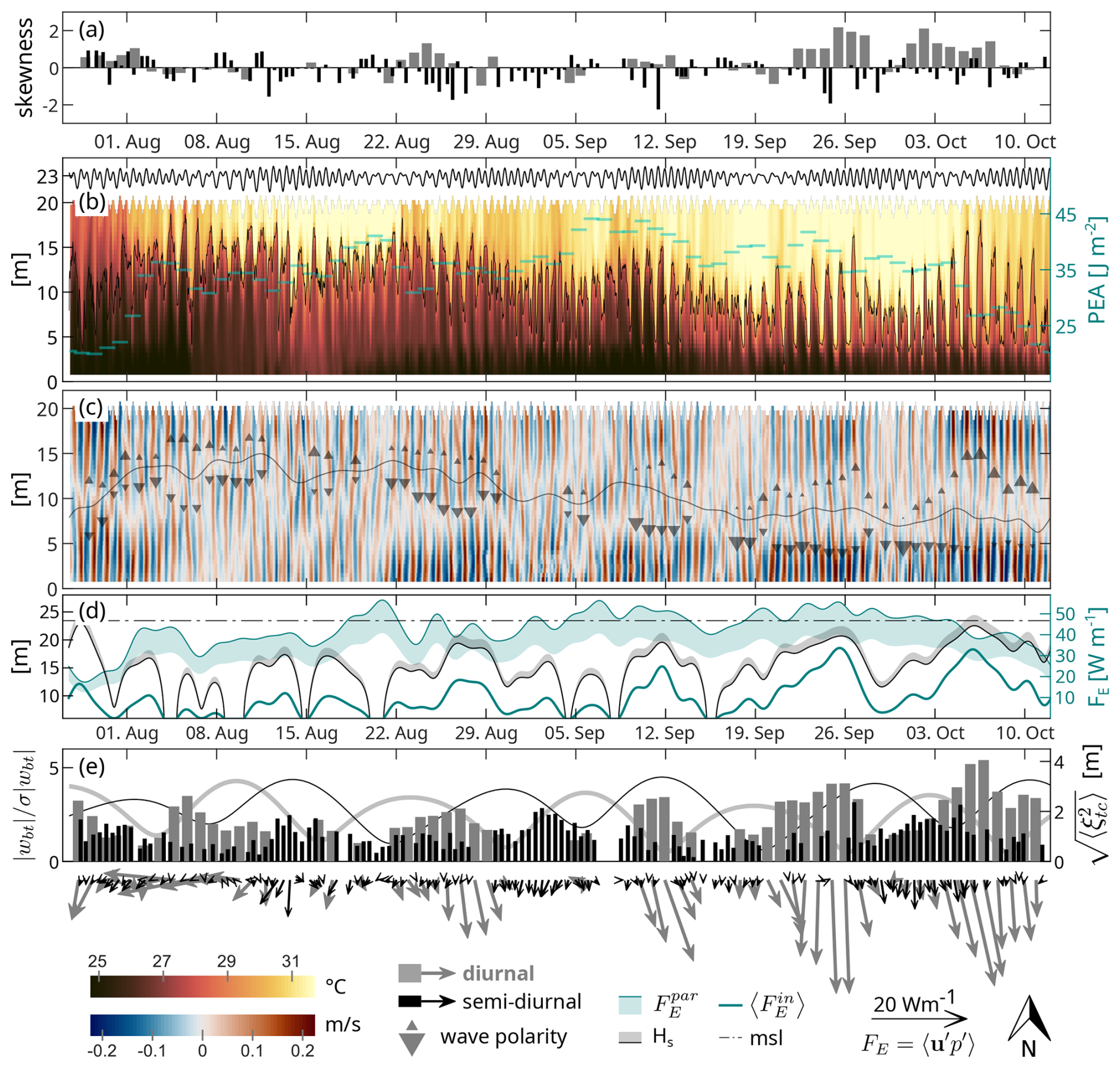
Figure 3 Mooring data during summer 2022 at station ISQ. (a) Skewness of $\mathrm{d}\mathit{\xi }/\mathrm{d}t$ (positive indicates steeper leading edges, negative indicates steeper trailing edges). (b) Sea level (from ADCP pressure sensor), vertical temperature profile, instantaneous z_TC (grey line), and daily averaged Potential Energy Anomaly (PEA, cyan). (c) Baroclinic cross-shelf currents (coloured) with low-pass filtered z_TC (grey line) and triangles at local extrema of the diurnal band-passed thermocline (troughs are indicated pointing down, scaled by the ratio trough/crest and crests pointing up, scaled by the ratio crest/trough). The two triangles of one IT indicate polarity and its magnitude. (d) Total low-passed incoming energy flux at ISQ together with ranges for parameterized energy flux and saturation depth H_s calculated after (Becherer et al., 2021b). (e) RMS of ξ (bars) and vectors representing baroclinic energy flux in geographic orientation; background lines show normalized amplitude modulation (K₁+O₁, gray and M₂+S₂, black) of the barotropic tidal transport converted to vertical velocity w_bt at the local shelf slope. Variables in panels (a) and (d) are decomposed into D- (grey) and SD- (black) components, y axes in panels (b)–(d) indicate height above ground.

After mid-August, the mean z_TC gradually deepens. During this period, the Potential Energy Anomaly (PEA) remains, on average, around 35 J m⁻², until stratification declines towards winter conditions in early October. The peak and depth-averaged values of the buoyancy frequency N² are typically of order 10⁻² and ${\mathrm{10}}^{-\mathrm{3}}{\mathrm{s}}^{-\mathrm{2}}$, respectively (Fig. 2c). Similar summer values of $N^{\mathrm{2}}\sim {\mathrm{10}}^{-\mathrm{2}}{\mathrm{s}}^{-\mathrm{2}}$ have been reported by Font et al. (2022) for the regional shelf slope, and in WOA climatological fields for the central GoO (Koohestani et al., 2023). Compared to other regions (e.g., compiled in Becherer et al., 2021b), the Al-Batinah shelf lies at the high end of global stratification intensity (in the absence of river plumes). With ADCP-derived shear typically of order $S^{\mathrm{2}}\sim \mathrm{5}\times {\mathrm{10}}^{-\mathrm{4}}{\mathrm{s}}^{-\mathrm{2}}$ and Richardson numbers $Ri>\mathrm{1}/\mathrm{4}$ during ∼ 90 % of the time, conditions across the thermocline remain predominantly stable.

In the tidal band (8–30 h), the cross-shelf baroclinic currents covary in intensity with the displacement of the thermocline (Fig. 3c), which reaches up to 14.5 m towards the end of the record. The recorded ITs displace between 40 % (25 August) and 60 % (5 October) of the water column. Both the root mean square of the thermocline displacement (ξ_rms) and, even more clearly, the energy flux F_E reveal the dominance of the D-band in the ITs (Fig. 3e). F_E in the SD-band is small compared to $F_{\mathrm{E}}^{\mathrm{D}}$ with $F_{\mathrm{E}}^{\mathrm{SD}}<\mathrm{5}\mathrm{W}{\mathrm{m}}^{-\mathrm{1}}$. ξ_rms and F_E, in both the D- and SD-bands, exhibit distinct fortnightly patterns (spring–neap cycles in the SD-band), with increasing intensity towards the end of the record. In ξ_rms, SD ITs appear particularly when their spring tides coincide with periods of low intensity in the D-band.

To represent local forcing, the amplitude modulation of the barotropic tidal transport, converted to vertical velocities at the local shelf slope $w={\mathit{u}}_H\cdot \mathrm{\nabla }h$, is shown separately for the D- and SD-bands, each normalized by its standard deviation (lines in Fig. 3e). The beat periods of the main tidal constituents are K₁+O₁: 13.7 d, and M₂+S₂: 14.8 d. As a result, the two fortnightly peaks shift their relative phase and during the record period, the two cycles are roughly out of phase. The fortnightly cycles of the ITs are less uniform than the astronomical forcing and exhibit delays of several days relative to the local barotropic forcing (Fig. 3e). The long time lags we observe between fortnightly peaks of local barotropic forcing and baroclinic signals point to remote generation. However, Gerkema (2002) demonstrates that frequency-dependent ray geometry (e.g., M₂ vs. S₂ beam angles) can produce strong spatial variations in baroclinic spring–neap phase, and that modest stratification changes can likewise induce large phase shifts. Horizontal interference, from separated generation locations, can furthermore produce spatially variable phase shifts in baroclinic fortnightly cycles.

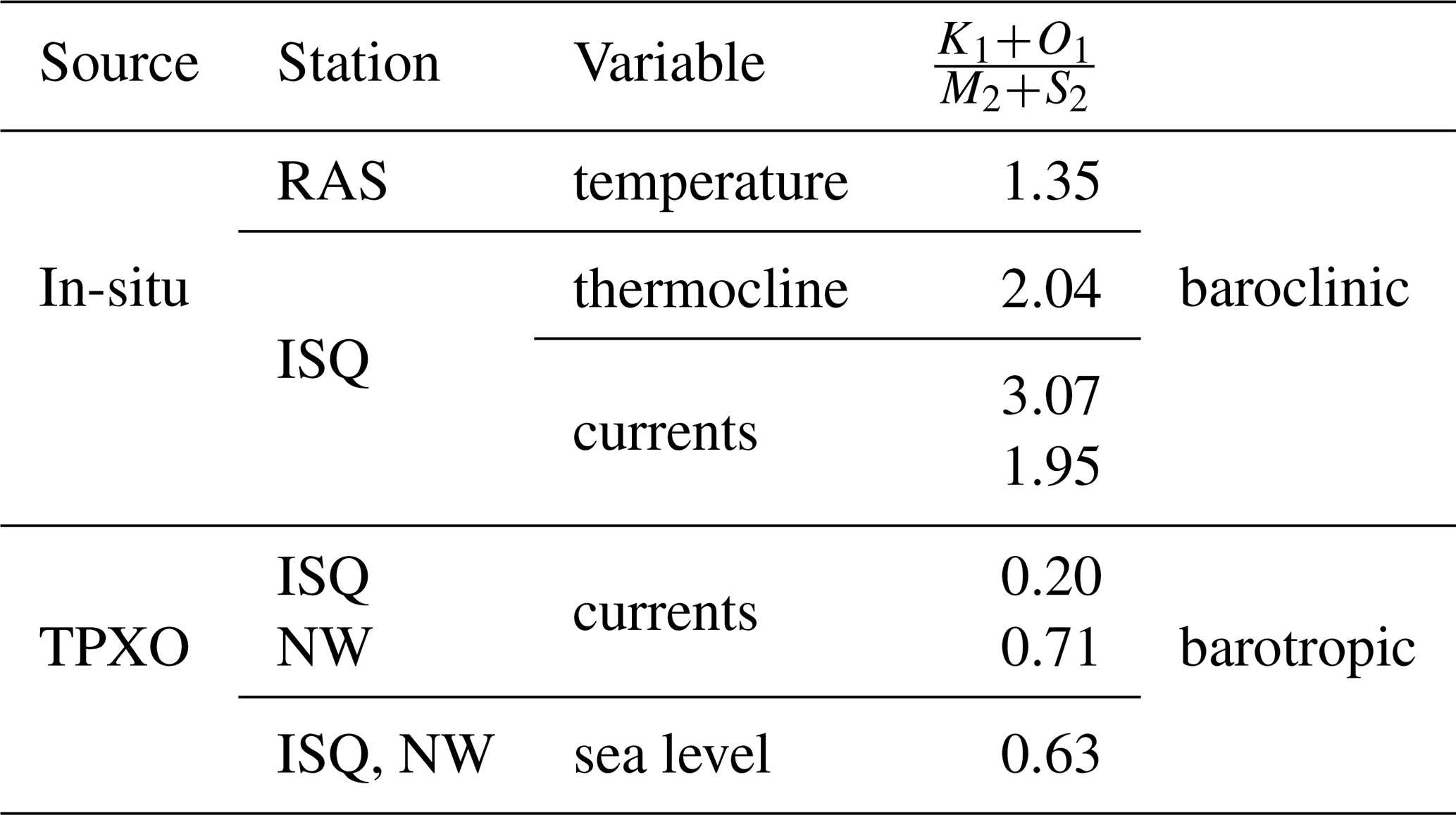
For the local barotropic transport at the Al-Batinah shelf slope, the SD-band is, in absolute terms, ∼ 4.5 times stronger than the D-band, marking a clear contrast with the observed ITs, where the D-band dominates (Table 1). Despite this discrepancy which could again be taken as indication for remote generation, local generation cannot be definitely ruled out from the data presented here as local shelf-slope topography could favor energy conversion in the diurnal band.

Table 1 Form number $\frac{K_{\mathrm{1}}+O_{\mathrm{1}}}{M_{\mathrm{2}}+S_{\mathrm{2}}}$ for temperature, thermocline displacement, and currents at stations RAS and ISQ from in situ measurements, and currents and sea level from TPXO tidal predictions at ISQ and NW locations. Values greater than 1 indicate D dominance, while values less than 1 indicate SD dominance.

Following restratification after the early August mixing/upwelling event, and from mid-August onwards, the IT energy flux is directed onshore. According to Siyanbola et al. (2024), this is again strong evidence for remote generation. The observed variability in the direction of the incoming diurnal IT energy flux (Fig. 1) further suggests remote generation and propagation effects, rather than purely local forcing. The variability we observe may result from multipath propagation, refraction by spatially and temporally varying stratification or mesoscale currents, and possible interference between remotely generated ITs. Gong et al. (2019) showed that remotely generated ITs can dominate and modulate local energy conversion on a shelf, altering both magnitude and direction of energy flux. Ansong et al. (2017) reported substantial temporal variability in SD IT energy fluxes driven by remote generation and propagation pathways. Therefore, the evolving flux directions in our data likely reflect remote IT sources, which are being refracted and temporally modulated before reaching the ISQ mooring. As mentioned above, from our data alone the question of remote vs. local generation can however not conclusively be answered and further analysis including the assessment of slope criticality, energy conversion and ray-beam modeling (which are beyond the scope of this study) will be necessary.

Several studies have reported the transformations long ITs undergo as they shoal on the inner shelf (e.g., Holloway et al., 2003; Colosi et al., 2018). Upon interacting with the seafloor, they develop increasingly steep waveforms, resulting in sharp bore fronts (McSweeney et al., 2020) and/or the generation of higher-frequency wave trains of ISWs/NLIWs. As ITs shoal on the sloping shelf, their amplitude eventually approaches the local water depth (Becherer et al., 2021b). In our data, we observe only the onset of bore-like features towards the end of the record, as ITs become increasingly asymmetric (slope skew) and eventually reverse their displacement polarity to waves of elevation in October. Low frequency variation of PEA is visible at approximately fortnightly periods with reduced stratification following periods of increased IT energy possibly suggesting mixing feedback. During typical summer conditions on the Al-Batinah Shelf, before z_TC starts to descend, onshore-directed F_E, generally stable stratification ($Ri>\mathrm{1}/\mathrm{4}$) and displacement amplitudes that remain small relative to the water depth at the ISQ mooring , however suggest that the primary dissipation of IT energy occurs shoreward from the 25 m isobath.

In order to quantitatively assess saturation of the ITs at the ISQ mooring, we calculate the parameterized energy flux $F_{\mathrm{E}}^{\mathrm{par}}$ and the saturation depth H_s as follows:

$$\begin{array}{}\text{(6)}& {\displaystyle }{F}_{\mathrm{E}}^{\mathrm{par}}={\displaystyle \frac{C_F{C}_A}{\mathrm{6}\mathit{\pi }}}{\mathit{\rho }}_{\mathrm{0}}{〈{\stackrel{\mathrm{‾}}{N}}^{\mathrm{2}}〉}^{\mathrm{3}/\mathrm{2}}{H}^{\mathrm{4}},\text{(7)}& {\displaystyle }{H}_{\mathrm{s}}={\left[{\displaystyle \frac{\mathrm{6}\mathit{\pi }}{C_A{C}_F{\mathit{\rho }}_{\mathrm{0}}}}\right]}^{\mathrm{1}/\mathrm{4}}\langle {\stackrel{\mathrm{‾}}{N}}^{\mathrm{2}}{\rangle }^{-\mathrm{3}/\mathrm{8}}\langle F_{\mathrm{E}}^{\mathrm{in}}{\rangle }^{\mathrm{1}/\mathrm{4}},\end{array}$$

according to Eqs. (10) and (15), respectively, in Becherer et al. (2021b). We use 36 h low-pass-filtered series of depth-averaged stratification $〈{\stackrel{\mathrm{‾}}{N}}^{\mathrm{2}}〉$ and total incoming energy flux $\langle F_{\mathrm{E}}^{\mathrm{in}}\rangle$ from our data, and the mean value of $C_A{C}_F=\mathrm{0.07}\times \mathrm{1.23}=\mathrm{0.083}$ for the coefficient product from Table 1 in Becherer et al. (2021b). To account for uncertainty, and because our local depth is at the shallow end of the range, we further use $C_A{C}_F=\mathrm{0.1}\times \mathrm{0.7}$ as bounding values.

Figure 3d shows the variation of $F_{\mathrm{E}}^{\mathrm{in}}$ versus $F_{\mathrm{E}}^{\mathrm{par}}$ and H_s in relation to the mean depth of 23.5 m. $F_{\mathrm{E}}^{\mathrm{in}}$ remains well below $F_{\mathrm{E}}^{\mathrm{par}}$ until the end of the record, when fortnightly peaks reach $F_{\mathrm{E}}^{\mathrm{in}}\approx \mathrm{30}\mathrm{W}{\mathrm{m}}^{-\mathrm{1}}$ and approach $F_{\mathrm{E}}^{\mathrm{par}}$, which by then has started to decrease with the relaxation of stratification. This indicates that the ITs remain mostly outside the saturation zone, and that the saturation depth H_s can be calculated reliably from the ISQ data.

The calculated H_s places the beginning of the IT surf zone at depths of around 15–20 m (4–7 km from shore), before increasing during the last two fortnightly peaks and approaching the local water depth at ISQ in October (Fig. 3d). Stratification and the z_TC level appear as primary constraints on the cross-shelf transport of IT energy. When stratification is weak and/or z_TC is low, dissipation occurs farther offshore; whereas under strong and shallow stratification, a greater fraction of energy reaches shallower sites. The strong summer stratification on the Al-Batinah Shelf appears to reduce displacement amplitudes sufficiently and provide a sufficiently strong waveguide (McSweeney et al., 2020) to allow ITs to propagate farther inshore than in other regions. For the shelf off central California, Becherer et al. (2021a) observe that the IT energy flux had decreased by at least an order of magnitude at the 25 m isobath, and conditions were inside the saturation regime. At comparable depths, both stratification and energy flux are lower on the California shelf compared to the Al-Batinah shelf.

During the final two recorded fortnightly packets in the diurnal band, both F_E and ξ_rms increase strongly. This rise does not follow the evolution of PEA, which is already decreasing, but coincides with the deepening of z_TC toward the seabed and with calculated H_s values approaching the local water depth, indicating that the ITs are entering a finite-depth shoaling regime. At the same time, the diurnal waves develop pronounced positive skewness and progress toward elevation polarity (Fig. 3a, c), which is characteristic of nonlinear steepening during IT shoaling on continental shelves (McSweeney et al., 2020; Becherer et al., 2021a, b). The simultaneous increase in ξ_rms and F_E is therefore consistent with the onset of shoaling-induced nonlinearity rather than with changes in stratification.

3.2 Waveform Structure

To characterize the waveform structure, we detail the baroclinic currents and isotherms for five periods with pronounced IT activity (Fig. 4). Both fields are band-passed over the entire tidal band (D- and SD-bands). The waveforms all deviate to varying extent from a purely sinusoidal shape expected under linear theory. Around 26 August when the mixed layer is shallow and the diurnal ITs are dominant, the peak isotherm displacement is larger downward with intensified near-bottom currents and the waveform has a steeper leading face (Fig. 4a). Around 3 September when ITs are pronounced semidiurnal, the waveform still resembles a depression wave but the slope asymmetry is sometimes reversed, with the steeper gradient now on the trailing face. Despite the clear SD signal in the displacement, the D-band is still prominently visible in the baroclinic currents. While the mean z_TC around 10 September is slightly lower, the diurnal wave patterns are still similar to the ones in late August. Around 25 September the mean z_TC further descended to below 10 m height and the downward displacement of the ITs extends close to the seafloor, increasing bottom influence on wave structure. The wave trough is flattened and the rising phase is further steepened. Eventually in October the polarity has reversed to higher upward displacements and a steepening of the falling phase.

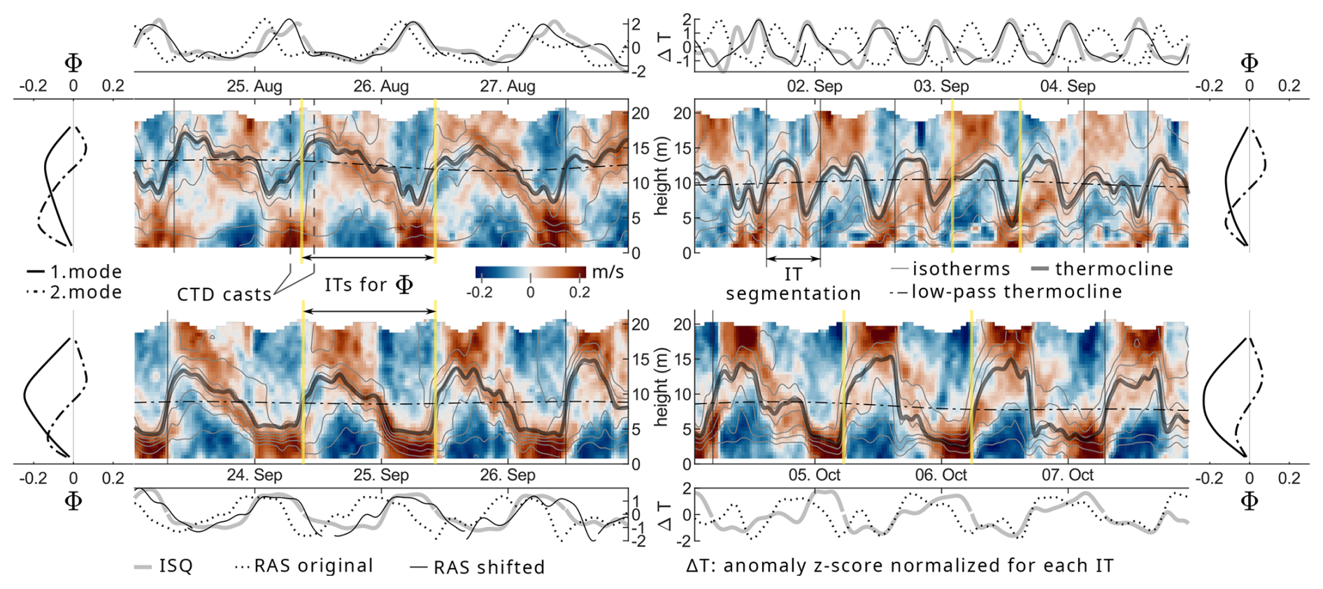
Figure 4 Baroclinic cross-shelf currents in the tidal frequency band (D + SD) for four selected ∼ 4 d intervals. Time of day is aligned across all time-series panels. Colours indicate currents (scale as in Fig. 3); thin grey lines are isotherms, thick grey lines represent instantaneous z_TC and dash-dotted lines show low-pass filtered z_TC. Vertical yellow lines mark one specific tidal phase used to determine the vertical modes. Outer panels show the first two vertical modes, scaled by the energy of currents projected onto pressure modes. Top and bottom panel rows show temperature anomalies of records at RAS and ISQ normalized for each wave segment. Dotted and solid lines indicate original and time shifted signals at RAS respectively.

Shroyer et al. (2009) describe polarity reversal of NLIWs with a shift to elevation waves when the pycnocline, which initially supports depression waves, becomes closer to the bottom than the surface. For shoaling depression waves that undergo polarity reversal, the trailing face can steepen. Similar to our observations, Cai et al. (2012) observe that with the mixed layer depth changing over the seasons, both elevation and depression waves may occur in the same region.

On 25 August, the phase relationship between the cross-shelf currents and the displacement is close to quadrature as would correspond to linear wave dynamics (e.g. Cushman-Roisin and Beckers, 2011). This phase relation is however restricted to the currents within a few meters around z_TC. Currents in lower layers are phase shifted indicating the influence of higher modes. At the end of September and the beginning of October, isotherm displacement and currents across the whole water column are in phase. This is consistent with the transformation of the ITs into bore-like shapes. Duda et al. (2004) assesses phase relation between baroclinic currents and displacement and links deviations from quadrature to increasing nonlinearity during the shoaling of D-band ITs. Similar to our observations, Becherer et al. (2021b) describe peaks in near-bottom currents as part of steep mode-1 internal tidal bores.

The dynamic vertical modes shown in the right column of each panel were derived from N²(z) profiles at z_TC zero-crossings, normalized and scaled by the energy of baroclinic currents projected onto each mode. These mode shapes represent the vertical energy distribution within the tidal band for each period. In late August and early September, energy is distributed between the first and second modes, corresponding to observed vertical shear and phase shifts indicating higher-mode contributions. In contrast, from late September onward, the first mode increasingly dominates, with second-mode contributions diminished. The shift toward dominance of the first mode in late September and October coincides with the observed deepening of the thermocline (cf. Fig. 3), suggesting that stratification weakening favors lower-mode vertical structures. This evolution toward first-mode dominance, waveform steepening, and coherent vertical structure is consistent with increasing nonlinearity during IT shoaling. McSweeney et al. (2020) similarly observe steepening and vertical structure evolution tied to stratification and bore feedback on the Central California Shelf. Duda and Rainville (2008) observe that as diurnal ITs propagate upslope, they exhibit current minima near the center of the water column, indicating that the energy organizes predominantly into mode-1. They observe nonlinear steepening during upslope propagation, particularly at shallower mooring sites, with sawtooth-like waveforms and bore-like fronts reported as signatures of nonlinear deformation.

The increased mode-1 dominance and waveform steepening we observe in early October align closely with increases in IT amplitude and skewness identified earlier (Fig. 3), highlighting nonlinearity as a primary factor shaping wave evolution. The observed onset of bore-like structures and first-mode intensification may enhance near-bottom mixing, consistent with the transient reductions in PEA (cf. Figs. 3b and 5c).

In the absence of spatial data, we do not apply KdV models to our IT observations. However, others have done so successfully; for example, Holloway et al. (2003) used a modified KdV framework to model IT propagation on the NW Australian shelf. The nonlinear features we observe, such as wave steepening, polarity reversal, and changes in vertical structure, are consistent with established nonlinear internal wave dynamics (e.g., Shroyer et al., 2009; Cai et al., 2012), suggesting that a KdV-type framework could be appropriate for future spatially resolved analyses.

3.3 Cross-shelf Coherence

Cross-shelf coherence measures how consistently IT signals are preserved between offshore and inshore locations, offering insight into their propagation pathways and the degree of energy loss or transformation across the shelf. Figure 5 shows the temperature recorded at the shelf-edge mooring (RAS) together with a temperature time series taken at the same vertical level (18 m depth) from the thermistor chain at the inshore station (ISQ). At the beginning of the period, the influence of the ITs at 18 m is small (though still clearly distinguishable), until the thermocline descends in late August (cf. Fig. 3b, c) and the isotherm displacement more prominently reflects in the fixed-depth temperatures.

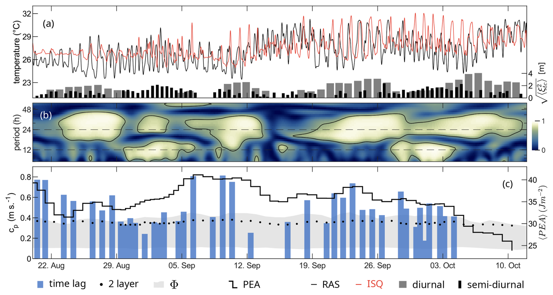
Figure 5 Cross-shelf coherence analysis. (a) Temperature time series at 18 m depth from stations RAS (black) and ISQ (red). Bars represent ξ_rms for the D- (grey) and SD- (black) components, as shown in Fig. 3e. (b) Wavelet coherence between the two temperature series, emphasizing the tidal frequency band (D- and SD-periods are marked by dashed lines). (c) Phase speed based on time lags between RAS and ISQ (blue bars), derived from modal analysis (shaded grey area) and two-layer model (points). Phase-averaged PEA (solid black line) is shown on the right y axis.

The pattern of high wavelet coherence between the two temperature time series matches with the periods of high IT energy in each of the tidal bands (bars of ξ_rms, Fig. 5a) which indicates that the propagation of the ITs can coherently be tracked from the shelf edge to the 12 km distant mid-shelf location at ISQ until the end of September. This confirms that dissipation and the corresponding discoherencing of the ITs happens inshore of ISQ. High coherence generally suggests near-linear wave propagation and the dominance of a single propagation direction during the event (not necessarily constant over longer periods).

The time lag between RAS and ISQ was determined through cross-correlation for individual waves identified in the extended tidal band (6–36 h; examples in top and bottom panels of Fig. 4). As before for the IT segmentation and F_E, only clearly identifiable waves and periods with high coherence were included in the analysis. The observed time lags range from 2 up to 8 h with lower time differences for the D-band. Phase speeds were determined from the time lags and the effective distance between the stations projected on the direction of the corresponding IT energy flux (cf. vectors in Fig. 3). We assume that the horizontal direction of the energy flux coincides with the horizontal phase propagation direction, which holds for linear internal waves in a horizontally homogeneous, weakly dissipative medium without significant background shear or refraction (Cushman-Roisin and Beckers, 2011). While both the time lags and the direction of the energy flux vary over the observed period, the estimated phase speeds exhibit an interpretable pattern.

On average, the phase speed from the time-lag method ranges around 0.5 m s⁻¹ which is slightly above the high end from modal analysis (diurnal mode-1, Fig. 5c). The c_p from SD ITs (29 August–6 September and before 3 October) are only marginally lower on average compared to the D ITs. The long-wavelength speed for an idealised two-layer system (see Sect. 2.5) ranges slightly below the highest mode speed (Fig. 5c).

The c_p we observe via the time-lag method exceed the mode-1 values at certain times while during other periods the differences are small. McSweeney et al. (2020) show that internal bores can deviate from linear speed estimates in the shoaling zone, relating to nonlinearity and waveguide modification. Martini et al. (2013) and Duda et al. (2004) similarly derived speeds of ITs from signal lags between moorings over the slopes of the Oregon and South China Sea shelves, respectively. While the observed M₂ speeds in depth >1000 m over the Oregon slope only match the lower speeds of mode-3, which Martini et al. (2013) attributed to mode scattering, the O₁ phase velocities of 1.14 m s⁻¹ observed between 80–350 m by Duda et al. (2004) are comparable to mode-1 c_p estimates. The high phase speeds we observe appear mostly during periods of enhanced stratification as indicated by PEA. Underestimation of stratification sharpness during these periods could be a potential cause for smaller modal speeds. Other potential reasons for the higher-than-mode-1 c_p we observe are advection by background flow (Xie et al., 2015), interactions with the barotropic tide (Stephenson et al., 2016), or cross-shelf flow due to the regionally pronounced land–sea breeze in the D-band.

Before 3 October, peaks in internal wave c_p coincide with periods of increased stratification, as indicated by higher PEA, while reduced stratification (low PEA) corresponds to lower c_p. Until the end of September, waveforms are similar in the temperature records of the two stations, and time lags are estimated by cross-correlation over entire individual wave phases. During the last recorded fortnightly IT pulse around 5 October, such time-lag estimation is no longer possible. The rising phase of temperature (i.e., isotherm depression) appears approximately in phase between the two stations (cf. lower right panel of Fig. 4), while the cooling phase is delayed inshore. This coincides with nonlinear steepening into bore-like structures, characterized by increased amplitude and polarity reversal of the incoming ITs. At this time, the vertical level used (18 m depth, 5 m above bottom at ISQ) is no longer suitable for tracking time lags.

Wavelengths were derived from the time-lag phase speeds and the individual periods of the identified IT waves. Wavelengths in the SD- and D-bands are concentrated between 15 to 25 and 40–50 km respectively, which falls within the range of other observations on shelves for comparable latitudes (Holloway et al., 2003; Wang et al., 2022). The distance between RAS and ISQ is around 20 km and thus smaller than the wavelength which likely explains the high coherence. Duda et al. (2004) consider the ratio of particle velocity to phase velocity $u_{\mathrm{r}}/c_{\mathrm{p}}$ as a measure of nonlinearity. In our case the ratios range up to ∼ 0.5 and while these values are below unity, they are nonetheless sufficiently large (and substantially larger than reported by Duda et al., 2004) to be associated with nonlinear effects as discussed in previous sections.

3.4 Spectral analysis

Figure 6 displays amplitude spectra for temperature, vertical displacement, and currents. As we have identified remote generation as likely scenario for the local ITs, we include here for comparison TPXO tides from a location at the entrance to the Strait of Hormuz (NW; see Fig. 1) where IT activity has been observed (Pous et al., 2004; Small and Martin, 2002; Subeesh et al., 2025). It should be noted that remote here refers to a distance of only around 180 km away from the local shelf. Amplitude spectra (rather than power spectral densities) are used to allow direct comparison with amplitudes of astronomical tidal constituents from the TPXO model at ISQ and NW. The spectra represent the sum of FFT amplitudes from positive and negative frequencies. For the complex velocity time series (u+iv), this corresponds to the combined rotary components and is directly comparable to the major axis amplitude from tidal harmonic analysis. Clockwise motion is consistently dominant in the currents. For real-valued data, the spectrum is symmetric, and the same summation ensures consistency with constituent amplitudes from tidal harmonic analysis.

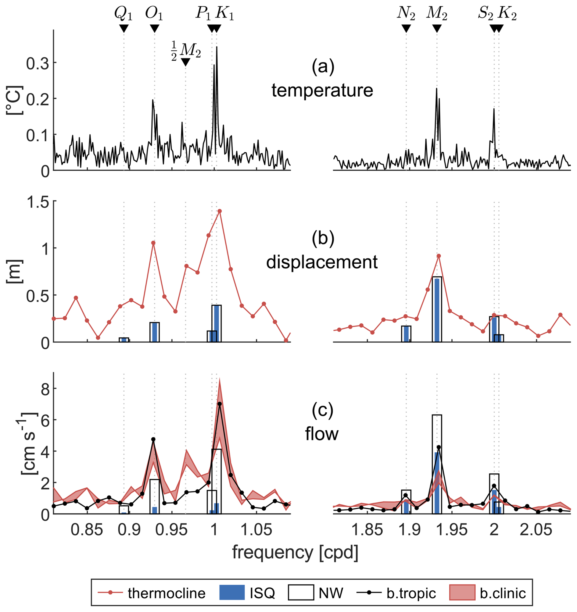
Figure 6 Amplitude spectra for (a) bottom temperature at station RAS, (b) thermocline displacement at ISQ (red line), and sea-level amplitudes of tidal constituents from the TPXO model at ISQ (blue bars) and at NW (white bars). (c) Barotropic (black line) and baroclinic (red shaded area indicates surface-to-bottom range) currents at ISQ, with major-axis tidal current amplitudes from the TPXO model (blue and white bars for ISQ and NW, respectively).

The spectrum of the 22-month bottom-temperature record at the shelf-edge station in RAS resolves distinct peaks at the main tidal frequencies and a smaller peak close to the $\mathrm{1}/\mathrm{2}{M}_{\mathrm{2}}$ frequency (Fig. 6a). Both lower resolution spectra from the 3-month data at ISQ, the thermocline displacement and the baroclinic currents, follow the general patterns of the temperature with dominant peaks at K₁ (and O₁) and a lower peak at $\mathrm{1}/\mathrm{2}{M}_{\mathrm{2}}$ (Fig. 6b–c).

The amplitudes of the sea-level constituents from TPXO are nearly identical between the local station ISQ and the remote location at NW, both dominated by M₂ (Fig. 6b). The major-axis amplitudes of tidal current ellipses derived from TPXO show that local astronomical tidal currents at ISQ are strongly dominated by M₂, even stronger than the sea level, with only weak energy in the D-band (Fig. 6c). In contrast, the D constituents at NW are comparatively strong, though still weaker than M₂. While the observed barotropic currents match with the local TPXO estimates at ISQ in the SD-band, the observations are much larger in the D-band.

Table 1 summarizes the predominantly diurnal variability in all in situ data whereas all data from TPXO exhibit form numbers <1, indicating SD dominance. This reflects a shift toward D dominance in internal tidal motions compared to the barotropic tide. Local TPXO currents are distinctly SD, and the measured barotropic currents appear influenced by ITs. Only at the remote NW site do TPXO currents show comparatively stronger D components.

Few studies report diurnal dominance in ITs which can only propagate equatorward of the critical latitude (∼ 30°); poleward of this limit, the diurnal tidal frequency is lower than the local inertial frequency, violating the dispersion relation ($f\le \mathit{\omega }\le N$) and causing the waves to become evanescent rather than freely propagating. Duda et al. (2004) report prominent diurnal ITs with a fortnightly cycle with an $O_{\mathrm{1}}/M_{\mathrm{2}}$ ratio increasing from 1 to 3 while propagating into shallow water at 22° N in the South China Sea. Rayson et al. (2021) observe K₁ dominance in ITs contrasting M₂ dominance in the barotropic tides at 18° S on the Australian North West Shelf in the Timor Sea. They explain the contrast as a result of seasonal stratification changes and standing wave interference that locally suppress M₂ and enhance diurnal constituents.

While the surface tide (sea level) within the western GoO is largely homogeneous, the barotropic transport has a constituent-dependent structure particularly near the entrance to the Strait of Hormuz where the $K_{\mathrm{1}}/M_{\mathrm{2}}$ co-range lines become perpendicular and diurnal tidal transport is enhanced (Small and Martin, 2002). Both Pous et al. (2004) and Subeesh et al. (2025) report strong K₁ energy and IT activity in the vicinity of the Strait of Hormuz near the NW location, pointing towards a potential remote generation site for the ITs we observe on the Al-Batinah Shelf. The distinct spectral peaks near the $\mathrm{1}/\mathrm{2}{M}_{\mathrm{2}}$ frequency that we observe might, on the other hand, be an indication of subharmonic resonance in local M₂ generation which can occur equatorward of 28.8° latitude (Gerkema et al., 2006).

3.5 Kinetic Energy

The ellipses shown in Fig. 1 were determined by least-squares fitting to the two decomposed components of baroclinic (all depths) and barotropic currents. The orientation of the major axis of the baroclinic component approximately corresponds to the general direction of the IT energy flux and is roughly orthogonal to the primarily alongshore orientation of the barotropic currents.

Figure 7a shows kinetic energy (KE) at ISQ, with the depth-averaged (barotropic) and baroclinic components derived from the tidal band signal 6–30 h as defined in Nash et al. (2012). Within the tidal band, baroclinic KE is pronounced in summer and retains approximately 10 % of the summer energy during winter. Barotropic KE is larger in winter and comparable in magnitude to the baroclinic KE observed in summer. The ∼ 20 % reduction of barotropic KE in summer is substantial enough to suggest seasonal modulation of the local barotropic tides, at least in terms of current strength. Potential causes for seasonality in barotropic tides include seasonal changes in barotropic energy loss during conversion to baroclinic tides (Li et al., 2012), stratification-induced changes in barotropic tidal transport (Müller, 2012) or tidal ranges (Li et al., 2012), and nonlinear barotropic–baroclinic coupling (Duda and Rainville, 2008). This seasonality has implications for harmonic analysis of the local barotropic tide, which we briefly address below in the context of predictability.

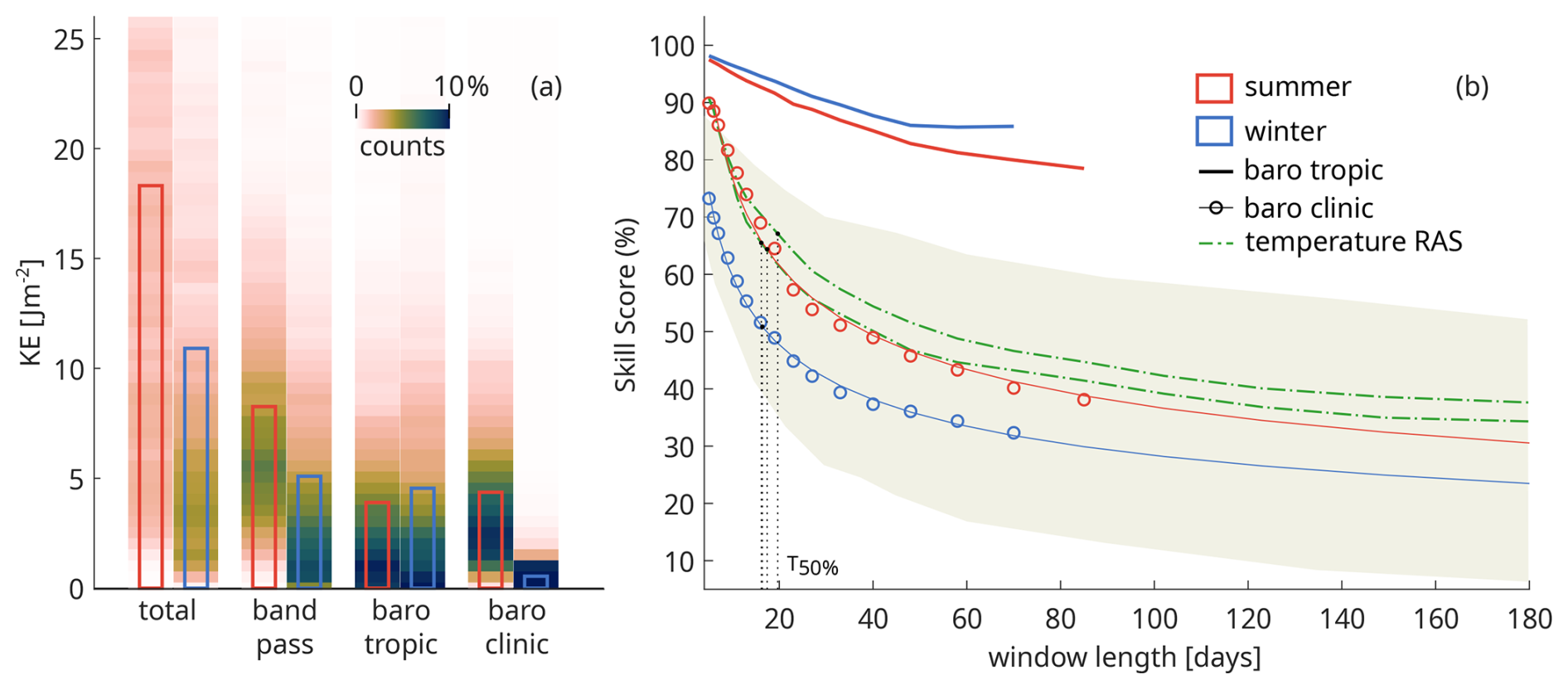
Figure 7 KE and IT predictability. (a) Depth-averaged KE at ISQ. Qualitative histograms of the temporal variation are shown color-coded, bars represent temporal means. Shown are total (unfiltered) currents as well as band-pass filtered (6–30 h) and decomposed components. Summer/winter periods are marked in Fig. 2. (b) Skill score (SS) for tidal prediction versus analysis window length. Thick lines represent barotropic flow, while markers represent baroclinic flow with power-law fits (thin lines). Blue tones correspond to winter, red tones to summer. Dashed green lines indicate bottom temperature at station RAS during two summer periods 2021 and 2022. Shaded area depicts the SS range from Nash et al. (2012) at 16 global sites.

The raw (total) summer KE is highly variable and, on average, significantly stronger than in winter (Fig. 7a). A longshore flow is observed in summer, which is vertically decoupled by stratification. The regional monsoon influence, as described by DiMarco et al. (2023) and Al-Al-Hashmi et al. (2019), induces a persistent low-frequency westward current over the local shelf. The high variability in the summer KE results from the background flow that elevates the mainly longshore barotropic tidal oscillations away from zero, thereby distributing KE over a wider range compared to similar currents in winter oscillating around zero.

3.6 Predictability

Predictability reflects how well IT phase and amplitude are maintained over time, and SS express this as the fraction of tidal-band variance captured by a harmonic fit, providing a basis for anticipating their effects on coastal mixing and transport. Figure 7b displays the SS as a function of the window length in days following the method described in Nash et al. (2012). SS variations for baroclinic conditions (currents at ISQ and temperature at RAS) in summer (April–October) and winter (December–February) can be directly compared to the range from Nash et al. (2012). We also show the same analysis applied to barotropic currents at ISQ in both seasons.

SS variations of all baroclinic signals exhibit similar shapes, albeit at different absolute levels. The two summer temperature records at the shelf break show the highest SS values, exceeding the upper end of the global range at short window lengths. In contrast, the SS of the baroclinic currents fall within the mid (summer) to lower (winter) part of the global range (Fig. 7b). Owing to the similar shapes of all SS curves, the derived T_50 % values are comparable across signals, supporting the robustness of the estimation. We find T_50 % between 16 and 19 d on the Al-Batinah shelf, which lies at the upper end of the 14 global sites for which Nash et al. (2012) report T_50 % values.

The region with the highest IT predictability in Nash et al. (2012), comparable to our observations on the Al-Batinah shelf, is the Timor slope of the northwest Australian shelf. Rayson et al. (2021) analyzed the ITs in this area using a Seasonal Harmonic Model. Similar to our results, they observe diurnal IT dominance at most stations despite M₂ dominance in the local barotropic tides, and attribute IT variability to seasonal changes in stratification and the presence of both local and remote generation. On the Al-Batinah shelf, our data also suggest a significant contribution from remote generation, which contrasts with the high SS. The two regions share general geographic features: both are semi-enclosed marginal seas located at similar latitudes. These parallels, and the similarity in the observed ITs, suggest that elevated IT predictability can persist under remote forcing in certain geographic configurations when supported by stable and coherent seasonal stratification.

We apply the same methodology to our barotropic currents at ISQ. For stationary barotropic tides, the SS curve is expected to remain high and nearly flat, with reductions arising mainly from unresolved constituents or short-term non-tidal variability (e.g., sea breezes) not represented in the harmonic fit. The SS of the barotropic tidal fits begins around 98 % for short windows but declines markedly with increasing record length (Fig. 7b). Harmonic analysis of a 2.5-month summer record yields a SS of approximately 85 %, while the shorter winter record levels off somewhat higher, at around 90 %.

The seasonal decline in barotropic predictability, particularly during summer, contrasts with the stationarity of unmodulated astronomical tides. This reduction likely reflects the influence of enhanced stratification, the presence of ITs, and possible observational cross-contamination in the summer records. These findings underscore the importance of accounting for IT activity and vertical structure when conducting harmonic tidal analyses of regional barotropic currents. Depth-averaged numerical models applied to this area have limited capability to reproduce realistic summer dynamics on the Al-Batinah shelf.

4 Conclusions

This study presents a detailed characterization of IT dynamics on the Al-Batinah Shelf, based on an 11-week mooring dataset encompassing the late summer stratification regime and its autumnal decline. A shallow summer thermocline with N² peaks up to $\mathrm{1}\times {\mathrm{10}}^{-\mathrm{2}}{\mathrm{s}}^{-\mathrm{2}}$ characterizes a highly stratified shelf environment that supports the shoreward propagation of coherent ITs beyond the typical internal surf zone. Parameterized comparisons following Becherer et al. (2021b) show that ITs remain largely below saturation at ISQ through late summer, with the surf-zone onset further onshore near 15–20 m depth.

Cross-shelf coherence and event-based phase speed estimates between 0.3 and 0.8 m s⁻¹ and wavelengths of 40–50 km (D) and 15–25 km (SD) demonstrate that ITs maintain coherence into the inner shelf, with observed phase speeds occasionally exceeding linear modal predictions. This discrepancy is attributed to nonlinear effects, stratification variability, and possible background advection.

In September, as z_TC deepens toward the seabed and H_s approaches the local depth, the ITs enter a finite-depth shoaling regime that enhances nonlinear steepening. Waveform structures indicate a transition from quasi-linear, depression-type waves to increasingly nonlinear waveforms, including steepening, skewness, and eventual polarity reversal – features consistent with bore-like evolution. Vertical modal analysis further confirms a shift from mixed-mode to first-mode dominance as the thermocline deepens and stratification weakens. This increase in nonlinearity is the primary driver of the late-season rise in local IT energy: during the final two diurnal fortnightly packets, both F_E and ξ_rms increase despite the onset of autumnal stratification decline.

The analyses of KE and predictability show seasonally modulated baroclinic activity and a 50 % reduction in predictability scores after T_50 %≈18 d, which is comparable to the higher end of global sites (Nash et al., 2012). Summer barotropic currents also show a marked reduction in longer-window predictability, potentially due to contamination by ITs and stratification-induced variability.

Spectral analysis confirms the diurnal dominance in IT variability and reveals a subharmonic peak near $\mathrm{1}/\mathrm{2}{M}_{\mathrm{2}}$, suggestive of local nonlinear interactions. The strong D-band dominance in the baroclinic tide contrasts with the locally M₂-dominated barotropic tide, and – together with multi-day lags between fortnightly IT amplitude modulation and barotropic transport over the shelf slope, as well as onshore-directed energy fluxes with ±10° variability in approach direction – points to a significant remote contribution to the local IT signal, though local generation cannot be conclusively excluded.

Together, these findings offer a coherent picture of IT evolution in a stratified marginal shelf setting and highlight the importance of nonlinear dynamics and remote forcing. Future work incorporating spatial observations and modeling will be necessary to fully resolve the propagation pathways and energy dissipation zones of the observed ITs.