Overlapping turbulent boundary layers in an energetic coastal sea

Turbulent mixing properties were directly observed to understand the interactions and overlapping events of wind-forced and tidally forced boundary layers in a deep, weakly stratified coastal sea. Te-Moana-o-Raukawa / Cook Strait of Aotearoa / New Zealand is an 𝒪(200 m) deep, energetic strait, known to experience both strong tidal currents and high wind speeds. More than 𝒪(40 000) quality-controlled turbulence observations were obtained from an ocean glider equipped with a microstructure profiler and a current speed through water sensor. Tidal flows of 𝒪(1 m s⁻¹) and wind speeds of 𝒪(10 m s⁻¹) independently enhanced turbulent dissipation to $\mathit{ϵ}=\mathcal{O}\left({\mathrm{10}}^{-\mathrm{5}}\mathrm{W}{\mathrm{kg}}^{-\mathrm{1}}\right)$ in bottom and surface mixed layers. Over a 4 d period, boundary-generated turbulence was evident in the interior water column on 10 occasions, enhancing interior diapycnal diffusivity levels by 5–35-fold, reaching K_z=𝒪(0.1–1 m² s⁻¹). In three instances, the surface and bottom mixed layers overlapped. These overlapping boundary layers were present in water depths 5-fold deeper than previously observed, which has implications for the vertical extent of material fluxes from the surface or seafloor. Interior stratification was transient, emerging from far-field advection of low-density surface water, and supported by vertical buoyancy fluxes that were episodically eroded by boundary-generated turbulence. Combining observations with one-dimensional General Ocean Turbulence Model (GOTM) outputs, turbulence interactions in the interior were found to be modulated by wind, tides, and transient stratification fields, in turn influencing the vertical structure of sinks and sources of turbulent kinetic energy. Enhanced vertical transport toward the interior of the near-boundary shear-produced turbulence was found to erode interior stratification. The interplay between antecedent stratification, turbulence generation, and vertical transport allows boundary layers to interact and modulate the vertical structure of seawater properties in deep coastal passages.

1 Introduction

Turbulent mixing regulates stratification, air–sea exchanges, and nutrient fluxes in the coastal ocean (Sharples et al., 2001; MacKinnon and Gregg, 2005; Bianchi et al., 2005). Variability in vertical and horizontal mixing patterns and mechanics has regional and global implications for biological productivity and the uptake of atmospheric carbon dioxide (Thomas et al., 2004; Borges et al., 2005; Simpson and Sharples, 2012; Becherer et al., 2022). Ocean turbulence is primarily focused in the surface and bottom boundary layers, where wind stress and tidal currents, respectively, generate turbulent kinetic energy (TKE) through shear-driven instabilities and wave breaking, leading to mixing (Waterhouse et al., 2014; Wang et al., 2014; Callaghan et al., 2014; Esters et al., 2018; Trowbridge and Lentz, 2018). Turbulence can be confined to each boundary layer independently but can also extend into the water column, leading to an interaction between the two boundaries. Surface and bottom boundary layers can overlap in shallow <𝒪(40 m) coastal waters (Gargett and Wells, 2007; Nimmo Smith et al., 1999; Schultze et al., 2020), but it is uncommon in the deeper ocean (Yan et al., 2022). Vertical separation of the boundary layers and/or inhibition by stratification within the water column interior are typically sufficient to prevent overlaps. Studying the stratification configuration and vertical turbulent exchanges that allow turbulent boundary layers to interact in deep passages is essential for understanding the extent to which mixing controls biophysical processes in all coastal ocean regions.

At the ocean surface, the boundary layer expands in relation to competing processes that either actively mix water properties (e.g. wind-driven shear instabilities, wave breaking) or increase stratification (e.g. solar heating, buoyancy fluxes). The balance of processes ultimately controls the transport of heat, gases, and mass across the air–sea boundary and into the ocean interior (Sutherland et al., 2014; Esters et al., 2018; Giunta and Ward, 2022). Near the seafloor, the bottom boundary layer originates from the complex interactions between oscillatory tidal currents, stratification, and seabed topography (Gayen et al., 2010). Each layer is characterised by elevated TKE dissipation rates (ϵ [W kg⁻¹]) and weak background stratification (N [s⁻¹]), termed the surface mixed layer (SML) and the bottom mixed layer (BML), respectively. In the SML and BML, quasi-homogeneous tracer concentrations illustrate the outcome of past mixing (Esters et al., 2018; Giunta and Ward, 2022). Representing actively mixing turbulence, ϵ is highest near the boundary, where TKE production is dominated by shear-driven processes, and usually decreases with distance to the boundary in each layer (MacKinnon and Gregg, 2005; Sutherland et al., 2014; Milne et al., 2017).

Based on the assumption that irreversible mixing rates and turbulent fluxes are dominated by large-scale turbulent kinetic energy production and eddy motions (Bouffard and Boegman, 2013; Osborn, 1980), diapycnal diffusivity (K_z [m² s⁻¹]), the measure of turbulence-driven diffusive fluxes across isopycnals, can be estimated from measurements of ϵ and N as

$$\begin{array}{}\text{(1)}& {\displaystyle }{\displaystyle }{K}_z\le \mathrm{\Gamma }{\displaystyle \frac{\mathit{ϵ}}{N^{\mathrm{2}}}},\end{array}$$

with Γ the efficiency coefficient for irreversible mixing, generally taken as 0.2, its canonical value, when direct estimates are not available (Gregg et al., 2018). Nevertheless, variation in Γ has been observed in numerical simulations, as well as in field and laboratory measurements. The cause of variability, particularly near surface and bottom boundaries, remains unresolved (see Monismith et al., 2018, for a comprehensive review). Fully developed isotropic turbulence is expected for $K_z>\mathrm{100}\times \mathit{\nu }\mathrm{\Gamma }\sim \mathrm{3}\times {\mathrm{10}}^{-\mathrm{5}}{\mathrm{m}}^{\mathrm{2}}{\mathrm{s}}^{-\mathrm{1}}$ (i.e. a buoyancy Reynolds number Re_b>100), with ν [m² s⁻¹] the kinematic viscosity (Schultze et al., 2017; Bouffard and Boegman, 2013; Shih et al., 2005). In the ocean interior, overlapping of boundary layers likely elevates ϵ and K_z from otherwise quiescent levels (Schultze et al., 2020; Yan et al., 2022), in proportions similar to those observed when e.g. internal waves break (e.g. interactions between boundary-produced turbulence and interior stratification) or when turbulence bursts are ejected from the boundary layers (Thorpe et al., 2008; Gayen et al., 2010; Zhang and Tian, 2014; Wang et al., 2014).

Using a large-eddy simulation (LES) of a 45 m-deep water column, Yan et al. (2022) concluded that in “intermediate-depth” ocean systems where surface and bottom boundary layers coexist, boundary layer overlapping can occur when interior stratification is weak and water depths are shallow. We employ a well-tested turbulence model (General Ocean Turbulence Model, GOTM, Burchard et al., 1999; Umlauf and Burchard, 2005) to isolate features of overlapping boundary layers in a deep, energetic system.

Directly observing turbulent dynamics of ocean boundary layers remains a challenge (Jabbari and Boegman, 2021). In recent years, ocean gliders have proven to be a robust platform for expanding understanding of ocean turbulence, largely due to the increased quantities of data. Gliders are autonomous underwater vehicles (AUVs) that use a buoyancy engine for locomotion and power-efficient remote sampling (Jones et al., 2005; Rudnick, 2016). The buoyancy propulsion engine means that gliders are relatively quiet platforms, well suited to turbulence sampling in a range of weather conditions, including strong winds (Fer et al., 2014; Peterson and Fer, 2014; Schultze et al., 2020). Sensors mounted on gliders allow for direct measurements of mean flow properties and turbulence-driven mixing dynamics.

Here, we present direct ocean glider observations and model evaluation of the dynamics of overlapping wind-forced and tidally forced boundary layers in an energetic coastal sea. The overarching objective of this work is to understand turbulent mixing dynamics when wind and tide-driven boundary turbulence interact in the interior, and the mixed layers overlap, raising the following questions: (1) what are the in situ turbulence characteristics of mixed layer overlapping? (2) What is the sensitivity of these characteristics to observing methods? (3) What is the vertical partition of turbulence sources and sinks when mixed layers overlap? (4) Finally, what are the implications of enhanced mixing driven by overlapping boundary layers for coastal ocean processes? The datasets and methodology are introduced in Sect. 2, and the observations and model results are presented in Sect. 3. In Sect. 4, the in situ observations and 1-D model outputs are discussed. Concluding remarks are provided in Sect. 5.

2 Methods

Overlapping boundary layers were examined using the following field and modelling approaches: (1) turbulence from an ocean microstructure glider (OMG), (2) flow conditions from a moored acoustic Doppler current profiler (ADCP), (3) wind forcing from an automatic weather station, and (4) turbulence balance terms calculated using the General Ocean Turbulence Model (GOTM), set up using observations from Te-Moana-o-Raukawa / Cook Strait.

The study site is a deep, wide, topographically complex passage that separates the two main islands of Aotearoa / New Zealand, Te-Moana-o-Raukawa / Cook Strait (Fig. 1). The central constriction, the Narrows Basin, is on average 210 m deep, 22 km wide, and 20 km long. It is a natural laboratory to study overlapping boundary layers, as it experiences both fast tidally driven flows with maximum $U\sim \mathrm{3.4}\mathrm{m}{\mathrm{s}}^{-\mathrm{1}}$ during spring tides and routinely has strong winds, exceeding 20 m s⁻¹ (Vennell and Collins, 1991; Stevens et al., 2012; Turner et al., 2019).

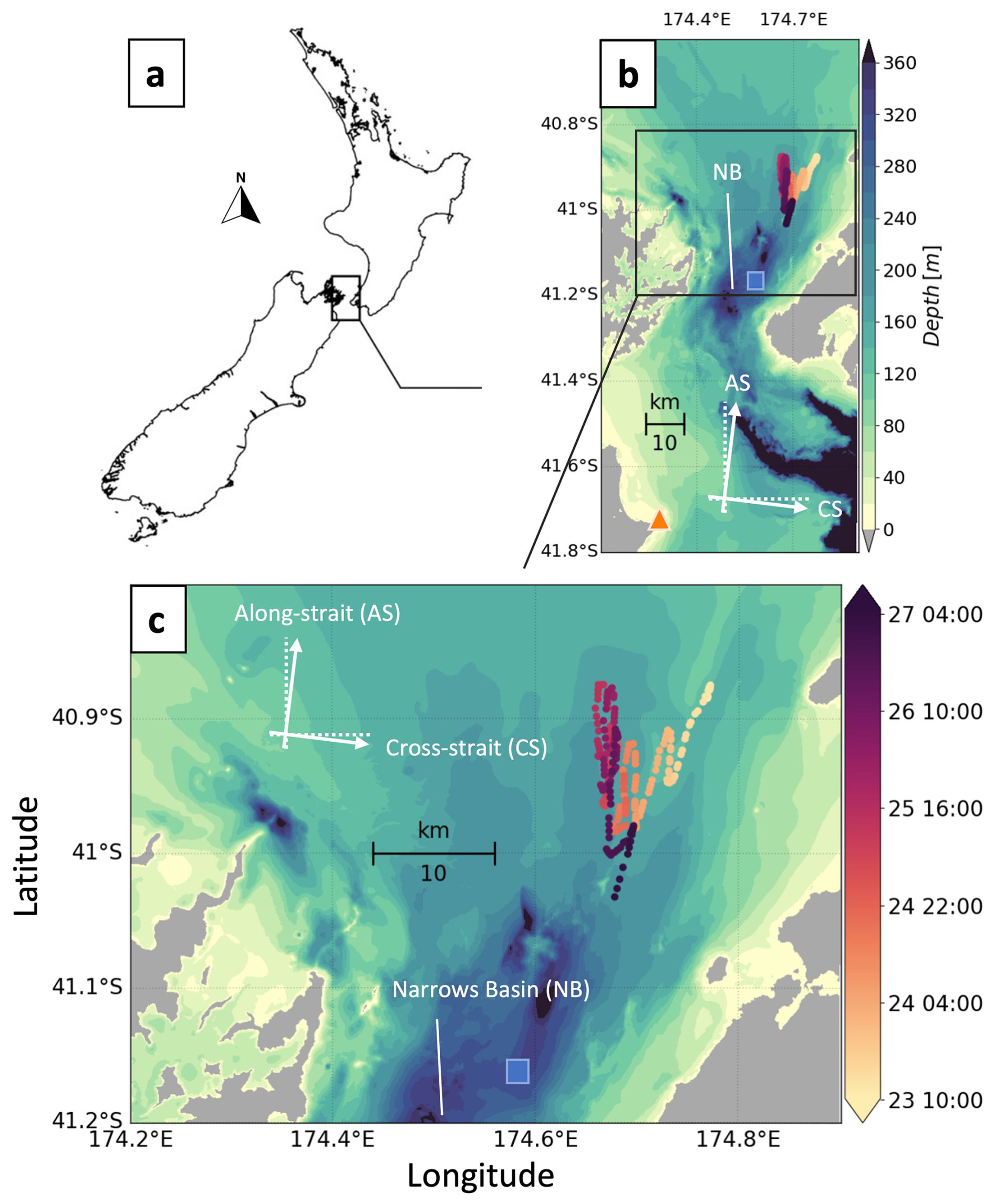
Figure 1 Maps showing (a) Aotearoa / New Zealand and (b) location of the ADCP (blue square marker), the Cape Campbell atmospheric sampling station (orange triangle marker), and the glider surfacing locations (coloured circular markers) and the topography of Te-Moana-o-Raukawa / Cook Strait (colour bar). (c) A zoomed-in window showing the current profiler and the glider surfacing tracks, coloured per time of the sampling window. In panels (b) and (c), the Narrows Basin and the along- and cross-strait directions are indicated in white.

Tidal currents in the Te-Moana-o-Raukawa / Cook Strait field region are primarily hydraulically driven by a 140° phase difference of the M₂ constituent across Greater Te-Moana-o-Raukawa / Cook Strait (Heath, 1986; Vennell and Collins, 1991; Vennell, 1998a, b). In addition, strong winds funnel through the strait, predominantly along the north–south axis, due to the narrow oceanic gap between mountain ranges on the Te Ika-a-Māui / North Island and Te Waipounamu / South Island (Vennell and Collins, 1991; Zeldis et al., 2013; Stevens, 2014). Stevens (2018) sampled turbulent mixing in the region over a 3 d period using a loose-tethered vertical microstructure profiler (VMP) and showed high levels of dissipation rates (linear average of $\mathit{ϵ}=\mathrm{2}\times {\mathrm{10}}^{-\mathrm{6}}\mathrm{W}{\mathrm{kg}}^{-\mathrm{1}}$) in a low stratification (${\mathrm{10}}^{-\mathrm{7}}<N^{\mathrm{2}}<{\mathrm{10}}^{-\mathrm{4}}{\mathrm{s}}^{-\mathrm{2}}$) environment. Environmental conditions of $<\mathrm{10}\mathrm{m}{\mathrm{s}}^{-\mathrm{1}}$ winds and $<\mathrm{1.5}\mathrm{m}{\mathrm{s}}^{-\mathrm{1}}$ mid water-column currents caused elevated diapycnal diffusivity (K_z) peaking close to 1 m² s⁻¹. Nevertheless, weak vertical stratification was found to persist in the strait (Stevens, 2014, 2018; Jhugroo et al., 2020), and boundary-driven mixing was not explicitly observed (Stevens, 2018).

2.1 In situ observations

Ocean glider and ADCP mooring observations (O'Callaghan and Elliott, 2022; Valcarcel et al., 2022) were obtained during June 2020 for Project CookieMonster (Cook Strait Internal Energetics MONitoring and SynThEsis Research), using the research vessel RV Kaharoa. The OMG completed a 20 d mission spanning 23 June–13 July. The moored ADCP was deployed at 41.1651° S, 174.5813° E for 6 d spanning 22–27 June. Herein, we focus on the 23–27 June 2020 period of concurrent OMG and ADCP sampling, when wind-forced and tidally generated boundary layers overlapped.

2.1.1 Glider-based turbulent microstructure

A Teledyne Webb Research Slocum glider was equipped with a MicroRider-1000EM turbulence profiler (Rockland Scientific Instruments) and a CTD (Sea-Bird Electronics), mounted on the top and side of the glider body, respectively. A relatively novel electromagnetic (EM) sensor was attached close to the shear probes on the nose of the MicroRider that directly measured flow past the sensors, providing an independent estimate of vehicle speed. A total of 257 co-located profiles of microstructure shear and temperature are presented here. Both up- and downcasts of microstructure were obtained; however, CTD profiles were only collected downward to conserve vehicle power. Each upward salinity profile (n) is estimated from the upward microstructure temperature profile (n) and the T–S relationship from the preceding downward profile (n−1).

High-frequency (512 Hz) measurements of the ∼5 mm-scale orthogonal ($\partial w/\partial x$, $\partial v/\partial x$) components of velocity shear in the reference frame of the glider, where the x coordinate is the glider path, were obtained using the two orthogonally mounted airfoil shear probes of the MicroRider (O'Callaghan and Elliott, 2022). Estimates of turbulent kinetic energy dissipation rates ϵ and kinematic viscosity ν were computed using the MATLAB codes developed by Rockland Scientific Instruments, the MicroRider manufacturer (RSI Odas library version 4.3.08, Lueck, 2016). Initially, isotropy of turbulence is assumed and implies that, for each probe, the dissipation rate of turbulent kinetic energy ϵ can be estimated from the shear spectra following Oakey (1982):

$$\begin{array}{}\text{(2)}& {\displaystyle }{\displaystyle }\mathit{ϵ}={\displaystyle \frac{\mathrm{15}}{\mathrm{2}}}\mathit{\nu }\stackrel{\mathrm{‾}}{{\left({\displaystyle \frac{\partial u_i}{\partial x}}\right)}^{\mathrm{2}}}={\displaystyle \frac{\mathrm{15}}{\mathrm{2}}}\mathit{\nu }\underset{\mathrm{0}}{\overset{\mathrm{\infty }}{\int }}\mathrm{\Phi }\left(k\right)\mathrm{d}k\left[\mathrm{W}{\mathrm{kg}}^{-\mathrm{1}}\right],\end{array}$$

where $u_i=\mathit{\{}v;w\mathit{\}}$ denotes the velocity components orthogonal to the path of the glider, and Φ is the shear spectra in wave number (k) space. Integration of shear spectra was computed in segments of 8 s with 4 s overlap and a 2 s fast Fourier transform segment length, yielding 54 300 ϵ estimates, with, on average, an estimate every 0.61 m.

Quantifying glider-based microstructure is a challenge, as the vehicle axial speed through the water, U, is generally computed using a glider flight model based on the pressure gradient and angle of attack of the vehicle (Merckelbach et al., 2010, 2019).

The use of in situ electromagnetic current metre data has been shown to improve shear-based ϵ estimates by 10 % in accuracy, where most U differences were attributed to flow variability (Merckelbach et al., 2019). To maximise confidence in the turbulence data for an energetic system like Te-Moana-o-Raukawa / Cook Strait, we collected direct electromagnetic current (EMC) measurements of speed past the sensors to quantify U. The EMC sensor (AEM1-G, JFE Advantech Co., Ltd) measured flow speed by electromagnetic induction (Hall effect) at an accuracy of 0.5 cm s⁻¹, assuming a 1 cm s⁻¹ reading uncertainty (Rockland Scientific, 2017; Merckelbach et al., 2019). The EMC measurements permitted raw counts to be converted into physical units of shear and frequency into wave number (k) for spectral analysis. The glider speed sensor estimates ranged from 0.05–0.55 m s⁻¹, averaging (±1 standard deviation) 0.34 (±0.04) m s⁻¹.

Unreliable ϵ estimates were removed from the analysis using the following criteria:

1. A minimum threshold for glider speeds of $U=\mathrm{0.20}\mathrm{m}{\mathrm{s}}^{-\mathrm{1}}$ filters out periods when the glider is not ascending/descending at a stable rate, removing sharp speed changes and inflexion points. This removed 14.8 % of total points.

2. If simultaneous ϵ estimates differ by an order of magnitude or more, the greater estimate is disregarded; otherwise, the average value of estimates is used (Scheifele et al., 2018). This removed 1.5 % of total points.

3. If glider speeds $U<\mathrm{5}(\mathit{ϵ}/N{)}^{\mathrm{1}/\mathrm{2}}$, i.e. lower than 5 times the turbulent flow velocities, Taylor's frozen field hypothesis is likely invalid (Fer et al., 2014), and ϵ is disregarded (Scheifele et al., 2018). This procedure removed 2.3 % of total estimates.

A total of 43 300 reliable ϵ estimates were used herein to examine overlapping boundary layers.

2.1.2 ADCP mooring and ancillary observations

The seabed mooring comprised an upward-facing ADCP (Nortek Instruments) and an SBE 37 conductivity–temperature–depth sensor (CTD, Sea-Bird Electronics). ADCP current velocities were sampled at 1 Hz, in 5 m bins between 35 and 295 m in water depth. Surface bins were discarded due to side-lobe interference. Velocities were filtered using an hourly first-order low-pass filter and decomposed into along- and cross-strait components (semi-major axis rotated 7° clockwise from true north, Fig. 1). Vertical shear was computed using the along- and cross-strait velocity components.

Hourly meteorological measurements from the Cape Campbell automatic weather station, ∼50 km away from the area of interest, were included in this analysis (Valcarcel et al., 2022). Along- and cross-strait components of wind speeds at 10 m above the water surface were then estimated using the Hellmann power law (Hellmann, 1919; Haas et al., 2021). Daily satellite averages of sea surface temperature (SST), with a 0.01° resolution (JPL MUR MEaSUREs Project, 2015), were also used to provide context to subsurface temperature patterns in the glider observations.

2.2 Mixing analysis

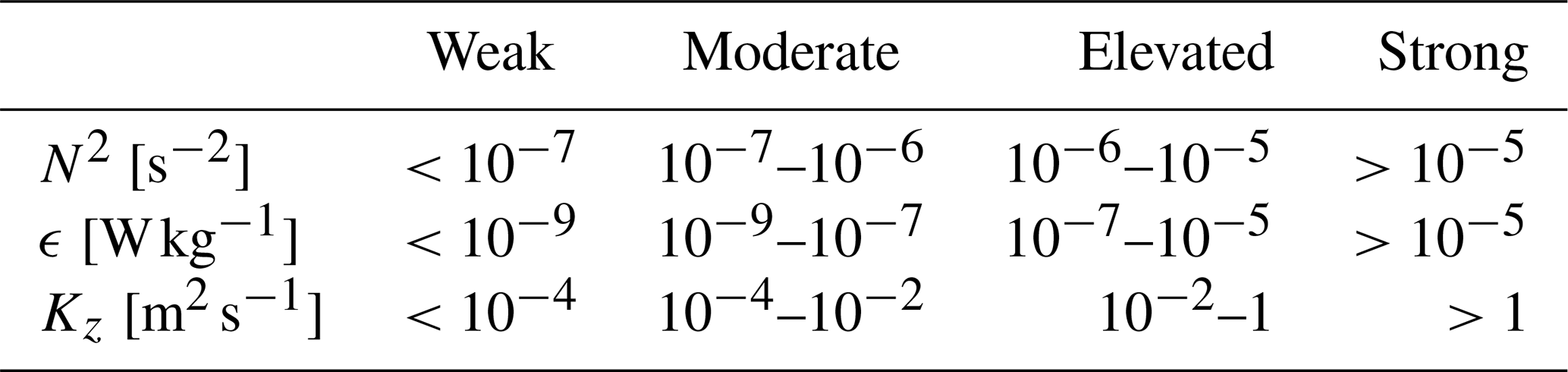
Potential temperature θ and density σ were computed from in situ measurements of temperature and practical salinity using the Gibbs SeaWater TEOS-10 formulation (IOC et al., 2010). Potential density profiles were re-ordered (σ^⋆) to be monotonically increasing with depth and used to compute the buoyancy frequency squared $N^{\mathrm{2}}=-g/{\mathit{\sigma }}_{\mathrm{0}}^{\star }\cdot {\partial }_z{\mathit{\sigma }}^{\star }$ [s⁻²] (Thorpe and Deacon, 1977; Mater et al., 2015), with g the gravitation constant and ${\mathit{\sigma }}_{\mathrm{0}}^{\star }$ the sorted potential density at a reference depth. For each profile, we identify the depths of the surface (SML) and bottom (BML) mixed layers, i.e. the top and bottom edges of the stratified interior layer, using a potential temperature threshold of Δθ=0.05 °C, assuming that it is a reliable proxy for homogeneity within a layer (Inall et al., 2021), as $z_{\text{top}}=z(\mathit{\theta }>{\mathit{\theta }}_{\mathrm{0}}-\mathrm{\Delta }\mathit{\theta })$ [m] and $z_{\text{bottom}}=z(\mathit{\theta }<{\mathit{\theta }}_{\mathrm{b}}+\mathrm{\Delta }\mathit{\theta })$ [m], where θ₀ and θ_b were the shallowest and deepest points in the profile, respectively. This temperature change broadly represents the separation between near-boundary, weak–moderate stratification, and interior elevated–strong N² (see Fig. 4 and Table 1). Overlapping mixed layers episodes are thus defined as periods when z_top>z_bottom.

Table 1 Reference table for the description of ranges of turbulent mixing variables in this study.

We further describe periods of turbulence interactions in the interior, when ϵ is enhanced above a threshold value, whether the mixed layers overlap or not. We arbitrarily assume that boundary-generated turbulence interacts in the interior during periods when fewer than 10 successive data points in glider profiles (∼6 m) are of weak dissipation, below ${\mathit{ϵ}}_p=\mathrm{3}\times {\mathrm{10}}^{-\mathrm{9}}\mathrm{W}{\mathrm{kg}}^{-\mathrm{1}}$. The ϵ_p threshold is an order of magnitude below the mean, $\mathrm{3.3}\times {\mathrm{10}}^{-\mathrm{8}}\mathrm{W}{\mathrm{kg}}^{-\mathrm{1}}$, and corresponds to the 15.8th percentile of the ϵ distribution, i.e. a standard deviation below the median, $\mathrm{1.1}\times {\mathrm{10}}^{-\mathrm{8}}\mathrm{W}{\mathrm{kg}}^{-\mathrm{1}}$. It was determined to be a relevant value for identifying periods of interior turbulence interactions in both the observations and the GOTM data presented in this study, and it is consistent with the commonly used dissipation thresholds for determining the extent of surface and bottom mixing layers (Sutherland et al., 2014; Esters et al., 2018; Giunta and Ward, 2022).

Diapycnal diffusivity is estimated through Eq. (1). Here Γ is set to 0.2, the canonical value for mixing efficiency. This choice is made because direct estimates of Γ are not available, and the community has not converged on a stable parameterisation of Γ in all oceanic turbulence conditions (Gregg et al., 2018; Monismith et al., 2018; Mashayek et al., 2022). Variations of Γ with turbulence activity (i.e. Re_b) have, however, been extensively documented and appear to represent well steady, homogeneous shear-driven turbulence (Shih et al., 2005; Bouffard and Boegman, 2013; Monismith et al., 2018). Therefore, to discuss the variations of diapycnal diffusivity in different Re_b conditions, we implement the Bouffard and Boegman (2013) parameterisation of K_z (applied to OMG observations in e.g. Schultze et al., 2017). Most (∼99 %) observations in the present study are of fully developed isotropic turbulence, i.e. Re_b>100. In this range, the Bouffard and Boegman (2013) parameterisation is $\mathrm{\Gamma }\equiv \mathrm{2}\times {\mathit{\text{Re}}}_{\mathrm{b}}^{-\mathrm{1}/\mathrm{2}}$ to estimate K_z with Eq. (1). The remaining samples are in the $\mathrm{7}<{\mathit{\text{Re}}}_{\mathrm{b}}<\mathrm{100}$ “transitional regime” range, for which Γ=0.2 is used in Eq. (1). For Re_b in 10³–10⁶ (90 % of points), parameterised Γ varies in the range of 0.07–0.002, differing from Γ=0.2 by 68 %–99 %. It should be noted that, within the mixed layers, near-boundary limitation of large overturning scales (i.e. large Re_b) may reduce Γ and K_z further, in unclear proportions (Bouffard and Boegman, 2013; Holleman et al., 2016; Monismith et al., 2018).

2.3 Physical separation of the sampling sites

The ADCP observations were used to provide a supplementary, semi-qualitative, tidal context to the OMG observations, and to scale the magnitude of tidal forcing in the GOTM simulations. The glider was, on average, 27.6 km from the ADCP (ranging from 19.7–35.9 km). Although separated by a relatively broad distance, we argue that shear and dissipation measurements can be qualitatively described within the same temporal framework, as the tidal excursion length characterising the system is large. The tidal excursion length, $L\equiv v_{\text{peak}}\cdot T_{M\mathrm{2}}/\mathit{\pi }$, ranged from 16.5–20.6 km and quantifies the distance over which a fluid particle travels at peak flow speed ($\left|v\right|\in \mathrm{1.2}$–1.5 m s⁻¹) during one tidal cycle (T_M2∼12 h), which was comparable to the average distance between sampling sites.

Depth-averaged currents sampled by the OMG were, on average, offset by 37 min from the moored ADCP measurements. This offset was more than double the phase lag determined by Vennell (1998a); however, the OMG data presented here were collected in a wider section of the strait, where flows were less constricted and the tidal wave propagation is slower. Depth-averaged currents sampled by the OMG were also 73 % of the amplitude of the ADCP measurements. This is most likely due to the flow constriction differences between the OMG and ADCP sites, the OMG site being significantly wider (Fig. 1). Using these considerations, background flow conditions for the OMG mission were inferred from the moored ADCP site, with a 37 min lag, and used to identify the periods of maximum and minimum shear. The 73 % amplitude scaling was used to prescribe tidal forcing to GOTM (see the following section).

Along a transect between the ADCP site and the mean glider location, the bathymetry shallows, and the channel width increases (Fig. 1c). Along this distance, the phase of the cross-sectionally averaged tidal velocity is approximately constant, characterising Te-Moana-o-Raukawa / Cook Strait as a non-divergent short strait (Vennell, 1998a, b). During southward tidal flows, hydraulic acceleration could be expected to differentiate turbulence properties between sites. During northward flows, a submerged pinnacle, Fisherman's Rock, lies just outside the edge of the westernmost glider sampling position and could affect turbulence structure by generating an eddy wake. For simplicity and to focus the analysis on boundary layer processes, these effects were not considered in this analysis.

2.4 General Ocean Turbulence Model

GOTM is a one-dimensional model that computes solutions for the vertical Reynolds-averaged Navier–Stokes equation for momentum and temperature and salinity transport equations. A choice of closure schemes is available to calculate turbulent tracer flux (Umlauf and Burchard, 2005; Umlauf et al., 2012). Here, the two-equation model (k−ϵ) solving for turbulent kinetic energy and a dissipative length scale (Canuto et al., 2001) was used. The turbulent kinetic energy (TKE, k) balance equation is represented by Reynolds decomposition in idealised Boussinesq fluid formulation (Polzin and McDougall, 2022; Umlauf et al., 2012) as

$$\begin{array}{}\text{(3)}& {\displaystyle }{\displaystyle }\dot{k}=T_k+P+G-\mathit{ϵ}\left[\mathrm{W}{\mathrm{kg}}^{-\mathrm{1}}\right],\end{array}$$

where $\dot{k}$ is the material derivative (includes temporal derivative and advection terms) of TKE. P, G, and ϵ are the rates of shear production, buoyancy flux, and dissipation of TKE, respectively. $T_k\equiv {\partial }_z\left(\mathit{\nu }{\partial }_{z}k\right)$, with ∂_z the vertical partial derivative. T_k, referenced hereafter as the “vertical transport” term, is the transport divergence and represents the contribution of all viscous and turbulent vertical transport terms (Yan et al., 2022; Becherer et al., 2022).

Behaviour of ϵ in a tidal- and wind-driven environment akin to Te-Moana-o-Raukawa / Cook Strait was examined. Model parameters were minimally tuned, similarly to the “Liverpool Bay” case used in the model development (Rippeth et al., 2001; Simpson et al., 2002; Verspecht et al., 2009). Salinity and temperature equations are solved with a 3 h timescale for relaxation to prescribed observations, interpolated to the GOTM time step. This timescale is representative of the mean duration of interior turbulence interactions and mixed layer overlapping events (3.4 h; see Table 2), and a “Liverpool Bay” case input (Rippeth et al., 2001). Horizontal velocity components, pressure, salinity, temperature, and TKE balance terms were computed over 100 evenly spaced levels of a 193 m depth (maximum water depth of the OMG data), with a 10 s integration time step. Scaled depth-averaged amplitudes of the dominant M₂ tidal flows were used to force the external pressure gradient from tidal constituents. Air–sea interactions at the surface boundary were forced by horizontal momentum fluxes, using wind stress time series (Watanabe and Hibiya, 2002). Air–sea heat fluxes are assumed secondary. However, relaxation to observed T–S observations is assumed to account for heat flux processes, e.g. night-time convection. Seabed interactions at the bottom boundary were prescribed with a typical bottom roughness length h_0b=0.004 m (i.e. hydrodynamical drag coefficient $C_d\sim \mathrm{2}\times {\mathrm{10}}^{-\mathrm{3}}$). Background values of ${\mathrm{10}}^{-\mathrm{10}}{\mathrm{m}}^{\mathrm{2}}{\mathrm{s}}^{-\mathrm{2}}$ and ${\mathrm{10}}^{-\mathrm{12}}\mathrm{W}{\mathrm{kg}}^{-\mathrm{1}}$ for k and ϵ were prescribed (Rippeth et al., 2001; Simpson et al., 2002; Verspecht et al., 2009).

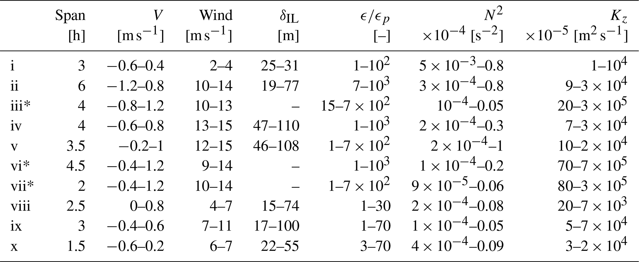
Table 2 Characteristics of interior turbulence interactions and mixed layer overlapping: duration (Span) and ranges of along-shore current (V) and wind (Wind) speeds, interior layer thickness (δ_IL), dissipation rate (ϵ), stratification (N²), and diapycnal diffusivity (K_z). The ranges of ϵ are scaled by ${\mathit{ϵ}}_p=\mathrm{3}\times {\mathrm{10}}^{-\mathrm{9}}\mathrm{W}{\mathrm{kg}}^{-\mathrm{1}}$, the criteria for identifying interior turbulence interactions (see details in text). Asterisks (*) indicate episodes that are also associated with mixed layer overlapping (black rectangles in Fig. 4).

3 Results

3.1 Background and forcing conditions

Flow speeds through Te-Moana-o-Raukawa / Cook Strait were dominated by the semi-diurnal spring tides, with along- and cross-strait speed components in the $\pm \mathrm{1.5}\mathrm{m}{\mathrm{s}}^{-\mathrm{1}}$ and $\pm \mathrm{0.5}\mathrm{m}{\mathrm{s}}^{-\mathrm{1}}$, respectively (Fig. 2a and b). The larger along-strait flows were oriented 7° from true north (not shown). Cross-strait tidal flows were ∼30 % slower but had greater vertical variability. The mean vertical structure of shear was similar for both directions of flow along the along-strait axis. Herein, we define the tidal phase of minimum and maximum bottom shear (mean of $\mathrm{1.6}\times {\mathrm{10}}^{-\mathrm{5}}$ and $\mathrm{3.9}\times {\mathrm{10}}^{-\mathrm{6}}{\mathrm{s}}^{-\mathrm{2}}$, respectively, in the deepest 20 m of the dataset), to qualitatively contextualise near-bed turbulence structure with the temporality of the background tides (Fig. 2c).

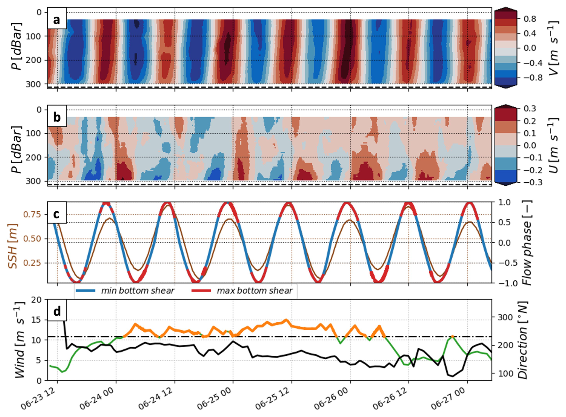
Figure 2 Large-scale forcing of turbulent mixing at the study site, a combination of fast tidal flows and a strong wind perturbation. The figure shows depth–time series of (a) along- and (b) cross-strait flow speeds (along the semi-major and semi-minor axes of the tidal ellipse, respectively); time series of (c) sea surface height (brown axis and line) and along-strait tidal phase (red and blue mark maxima and minima in bottom shear, respectively); time series of (d) wind speed below (green) and above (orange) the 10.8 m s⁻¹ threshold described in the text (dashed black line) and wind direction (from true north, black line), estimated at 10 m above sea level from Cape Campbell weather station records. In panels (a) and (b), the dashed line indicates the seafloor.

Wind speeds ranged from 2–15 m s⁻¹ over the period of the glider mission and mooring deployment (Fig. 2d). From 24 to 26 June, a 2 d event of strong south-westerly winds funnelled through the strait, with hourly wind speeds of 9–15 m s⁻¹, peaking during the last 4 h of 25 June. Low (green) and high (orange) wind periods were delineated using the 10.8 m s⁻¹ threshold, to distinguish periods of calm to fresh breeze conditions from strong breeze to near-gale winds, on the empirical Beaufort scale. These scale and criteria are consistent with the methods of Schultze et al. (2020), to facilitate comparison with turbulence generated under similar high-wind forcing conditions.

Daily averaged SST fields show a warm surface layer from Greater Te-Moana-o-Raukawa / Cook Strait advected southwards through the Narrows over the same period (Fig. 3c). Several occurrences of notable high temperature, low-density surface water (LDSW) were observed, likely related to the path of the glider crossing a surface front on several occasions (see also Fig. 4b). The vertical extent of LDSW was from the surface down to ∼100 m when observed by the glider.

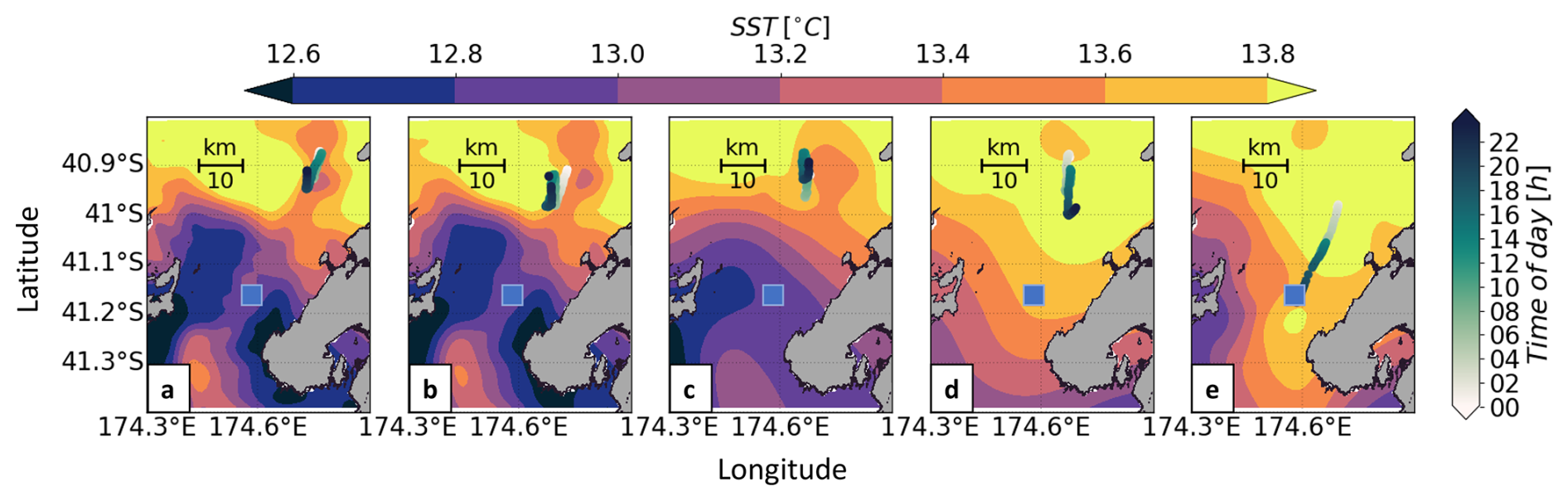
Figure 3 Overlay of OMG tracks and satellite-based SST measurements shows the connection between the observed “low-density surface water” and a larger-scale surface temperature front. Maps of Te-Moana-o-Raukawa / Cook Strait with satellite SST fields (horizontal colour bar), ADCP site (blue square marker), and OMG surfacing events by time of day (circular markers, vertical colour bar) for the days (a) 23, (b) 24, (c) 25, (d) 26, and (e) 27 June.

3.2 Boundary mixed layers and turbulence

Weakly stratified conditions were observed throughout the sampling period, with potential temperatures ranging from 12.5–14 °C, vertical gradients smaller than 1 °C, and N² below $\mathrm{5}\times {\mathrm{10}}^{-\mathrm{5}}{\mathrm{s}}^{-\mathrm{2}}$ (Fig. 4a–c). The average thickness of the surface mixed layer (SML) was 43 m and ranged from 10–139 m. The average thickness of the bottom mixed layer (BML) was 61 m and ranged from 22–150 m. The averaged N² for the SML and BML was 10⁻⁶ and $\mathrm{6}\times {\mathrm{10}}^{-\mathrm{7}}{\mathrm{s}}^{-\mathrm{2}}$, respectively (Fig. 4c).

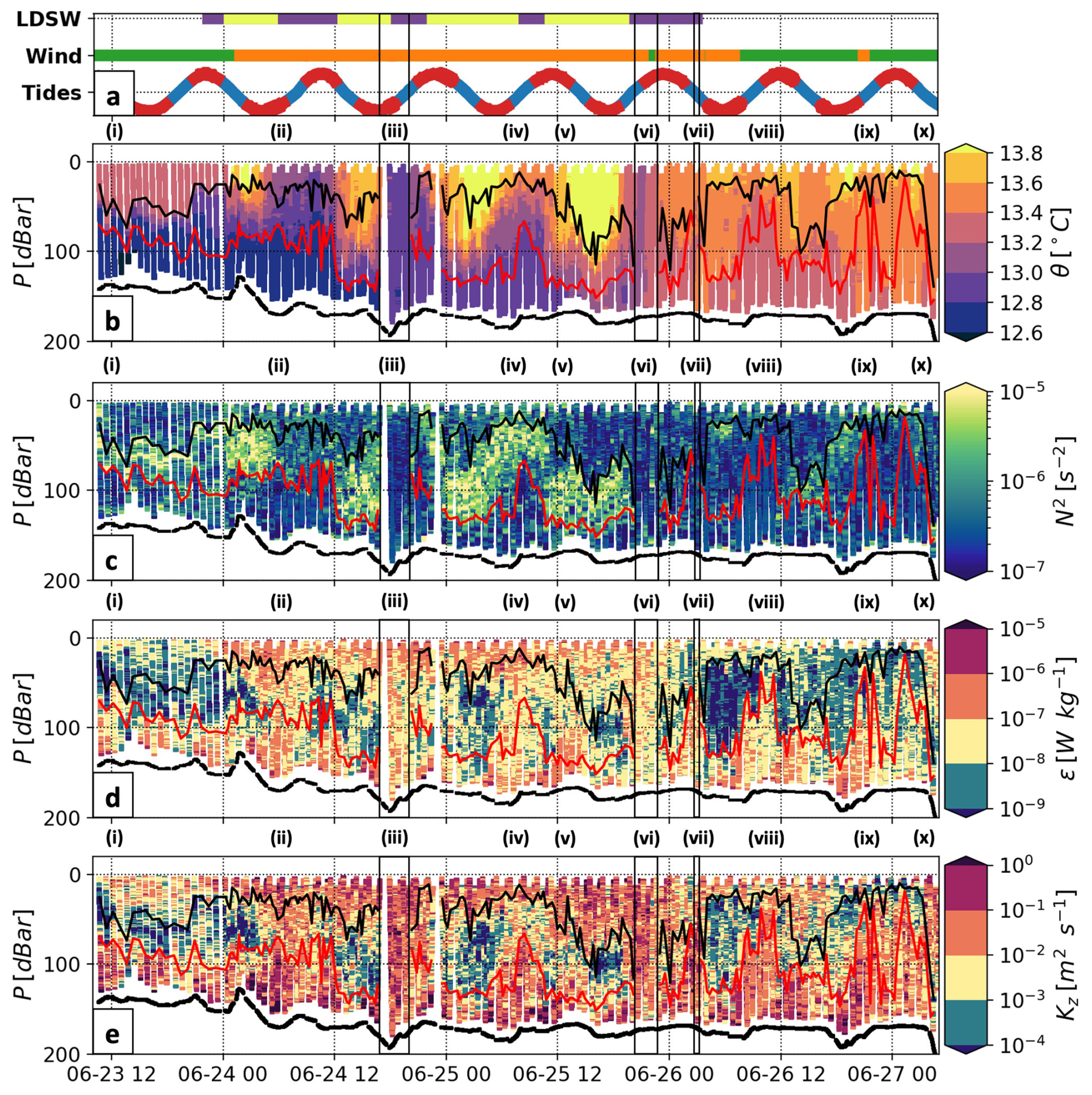
Figure 4 Variability of turbulence-driven mixing in a temperature-layered water column. Panel (a) shows the time windows for the low-density surface water (LDSW) episodes (purple and yellow top line), and bulk wind speed (green and orange middle line) and tidal shear (red and blue bottom sinusoid) variations. Panels (b)–(e) show the depth–time series of Ocean Microstructure Glider observations of (b) potential temperature, (c) buoyancy frequency squared, (d) dissipation rates, and (e) diapycnal diffusivity. For panels (b)–(e), the thick dashed black line is the seabed, and the surface (SML) and bottom mixed layer (BML) depths are shown with the black and red lines, respectively. For all panels, episodes of interior turbulence interactions are numbered (i–x), and the instances when mixed layers overlap episodes are marked with black solid rectangles.

Interior stratification was distinct from the SML and BML. Elevated N² values at the margins of the interior layer were $\mathrm{3}\times {\mathrm{10}}^{-\mathrm{6}}$ and $\mathrm{2}\times {\mathrm{10}}^{-\mathrm{6}}{\mathrm{s}}^{-\mathrm{2}}$, respectively (Fig. 4a–c). N² in the interior layer was up to 3-fold greater than either the SML or BML, with peaks co-located with strong temperature gradients. The interior layer had an average thickness of 63 m but was up to 125 m thick at times. Enhanced dissipation rates were observed in the SML and BML of Te-Moana-o-Raukawa / Cook Strait (Fig. 4d). Intensified surface turbulence was focused in the upper ∼50 m and mostly confined to the SML. High dissipation in the SML was in the elevated range, episodically, in the top 10 m. In the BML, there were elevated bottom-driven turbulence pulses with ${\mathrm{10}}^{-\mathrm{7}}<\mathit{ϵ}<{\mathrm{10}}^{-\mathrm{4}}\mathrm{W}{\mathrm{kg}}^{-\mathrm{1}}$ that ascended to 75 m from the seabed at the semi-diurnal tidal frequency. Lower levels of dissipation were typically observed in the interior layer of the water column.

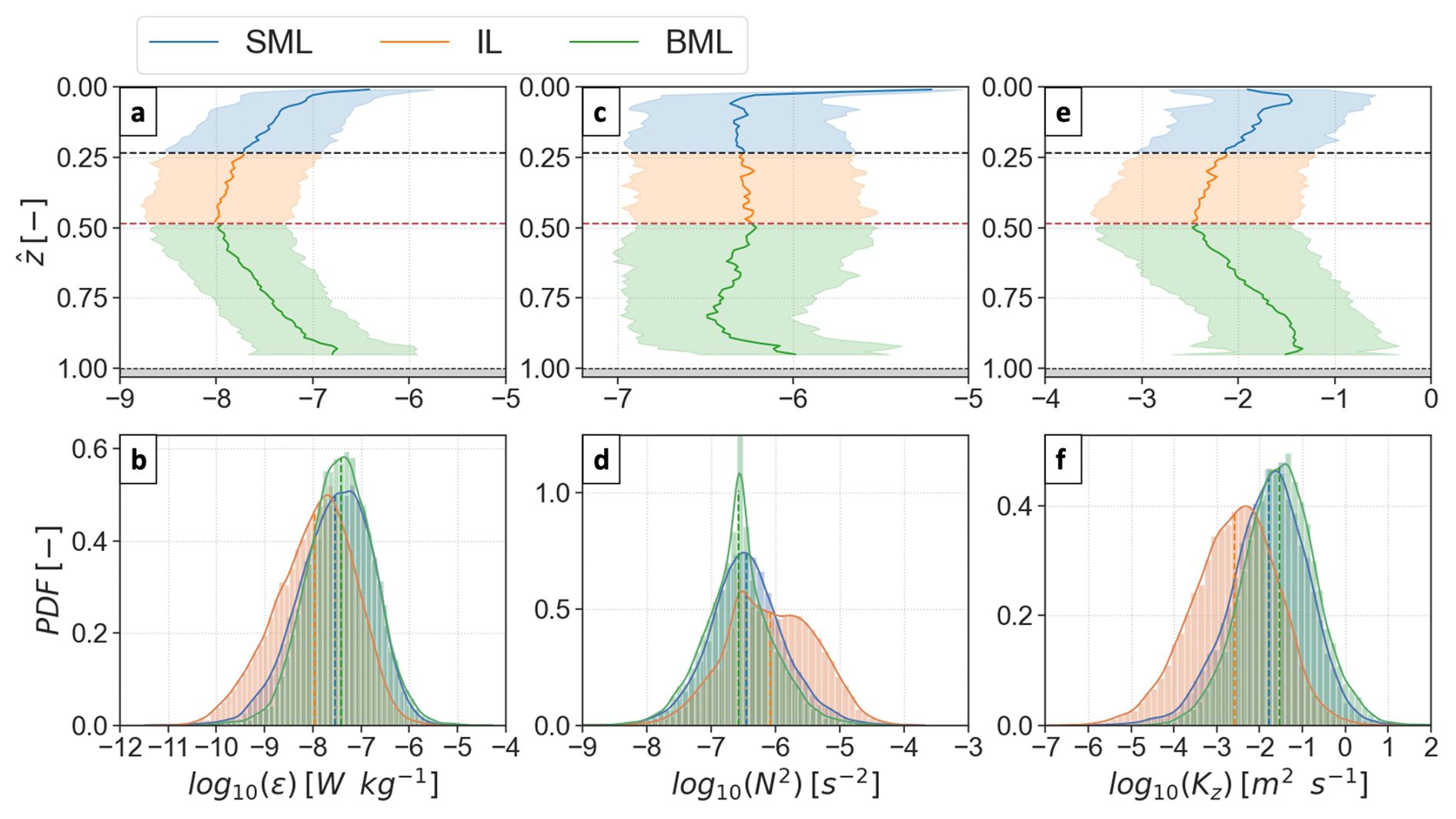
Figure 5 Log-averaged profiles along normalised water depth ($\widehat{z}$, a, c, e) and probability density function (PDF, b, d, f) of (a, b) dissipation rates, (c, d) buoyancy frequency squared, and (e, f) diapycnal diffusivity. In (a), (c), and (e), time-averaged mixed layer extents are represented. The time-averaged top (black dashed line) and bottom (red dashed line) depths of the interior layer (IL, green) delineate, indicatively of the mean surface (SML, blue) and bottom (BML, green) mixed layers. Dark lines indicate the mean values, and the lighter envelope shows the ±1 standard deviation intervals. In (b), (d), and (f), the SML, IL, and BML subsets are made of the instantaneous points for each glider profile. Solid lines indicate the curve fit of the underlying lighter coloured histograms and the dashed lines the mean value of each distribution.

Elevated–strong levels of canonical diapycnal diffusivity, K_z(Γ=0.2), were primarily observed within the mixed layers (Fig. 4e). Fully developed isotropic turbulence was observed for 98.9 % of samples, with $K_z<\mathrm{3}\times {\mathrm{10}}^{-\mathrm{5}}{\mathrm{m}}^{\mathrm{2}}{\mathrm{s}}^{-\mathrm{1}}$ only for 2.7 % of interior layer samples, and 0.4 % and none in the SML and BML, respectively. Diffusivity peaked to strong ($K_z>\mathrm{1}{\mathrm{m}}^{\mathrm{2}}{\mathrm{s}}^{-\mathrm{1}}$) levels less than <20 m from the seabed, where strong tidally driven ϵ pulses acted against weak stratification (Fig. 4c–e). In the SML, K_z levels were in the elevated–strong range during periods of intensified wind forcing, albeit with fewer strong samples than in the BML due to the relatively stronger stratification. When the mixed layers did not overlap, moderate–weak K_z was found in the interior, from the combination of moderate–weak dissipation and elevated–strong stratification.

The water column typically had intensified turbulence and diffusivity in both boundary layers and were highest in the BML (Fig. 5). The highest ϵ values were found in the first 10 % of the water depth, near each boundary, and decreased 10-fold over the mixed layer extent (Fig. 5a). SML and BML ϵ were log-normally distributed, log-averaging to $\mathrm{2.9}\times {\mathrm{10}}^{-\mathrm{8}}$ and $\mathrm{3.8}\times {\mathrm{10}}^{-\mathrm{8}}\mathrm{W}{\mathrm{kg}}^{-\mathrm{1}}$, respectively. Approximately 26 % (SML) and 27 % (BML) of observations had elevated–strong dissipation $\mathit{ϵ}>{\mathrm{10}}^{-\mathrm{7}}\mathrm{W}{\mathrm{kg}}^{-\mathrm{1}}$ (Fig. 5b). Moderate–weak stratification was found in the SML, averaging to $N^{\mathrm{2}}=\mathrm{3.6}\times {\mathrm{10}}^{-\mathrm{7}}{\mathrm{s}}^{-\mathrm{2}}$, and increasing near the surface–elevated values in normalised water depths ($\widehat{z}$) below 0.05 (Fig. 5c). Stratification depth-bin averages in the BML were weaker overall and varied more significantly, with a narrower distribution around a $\mathrm{2.7}\times {\mathrm{10}}^{-\mathrm{7}}{\mathrm{s}}^{-\mathrm{2}}$ mean (Fig. 5d). As a result, elevated–strong diffusivity (log-mean $K_z>\mathrm{0.01}{\mathrm{m}}^{\mathrm{2}}{\mathrm{s}}^{-\mathrm{1}}$) was found in the upper and lower 25 % of the water column (Fig. 5e).

Diapycnal diffusivity distributions were log-normal in both mixed layers but with a BML log mean (mean) of 0.03 (0.3) m² s⁻¹, which was twice as high as in the SML, as N² was lower overall (Fig. 5f). 70 % and 60 % of SML and BML samples were elevated–strong ($K_z>\mathrm{0.01}{\mathrm{m}}^{\mathrm{2}}{\mathrm{s}}^{-\mathrm{1}}$), much higher than in the interior layer (30 %), as N² was, on average, 2–3 times higher than in the mixed layers.

3.3 Overlapping mixed layers and interior turbulence interactions

Three overlapping mixed layers episodes were observed, when mid-water column diapycnal diffusivity was strongly enhanced (Fig. 4). Background stratification was moderate–weak during overlapping episodes, peaking at $\mathrm{2}\times {\mathrm{10}}^{-\mathrm{5}}{\mathrm{s}}^{-\mathrm{2}}$ during episode (vi) and otherwise reduced by 3–4 orders of magnitude (Table 2). Dissipation increased to 100–1000×ϵ_p throughout the water depth. This yielded strongly enhanced mid-water column diapycnal diffusivity, a minima $\mathrm{2}\times {\mathrm{10}}^{-\mathrm{4}}{\mathrm{m}}^{\mathrm{2}}{\mathrm{s}}^{-\mathrm{1}}$, and increased by 4–5 orders of magnitude to peak at 20 m² s⁻¹. For context, mean K_z reached $\mathrm{4}\times {\mathrm{10}}^{-\mathrm{2}}{\mathrm{m}}^{\mathrm{2}}{\mathrm{s}}^{-\mathrm{1}}$ in Gibraltar Strait, the canonical strait at this scale (Wesson and Gregg, 1994; Stevens, 2018), and $\mathrm{3}\times {\mathrm{10}}^{-\mathrm{5}}{\mathrm{m}}^{\mathrm{2}}{\mathrm{s}}^{-\mathrm{1}}$ for the upper 1 km of the global ocean (Waterhouse et al., 2014).

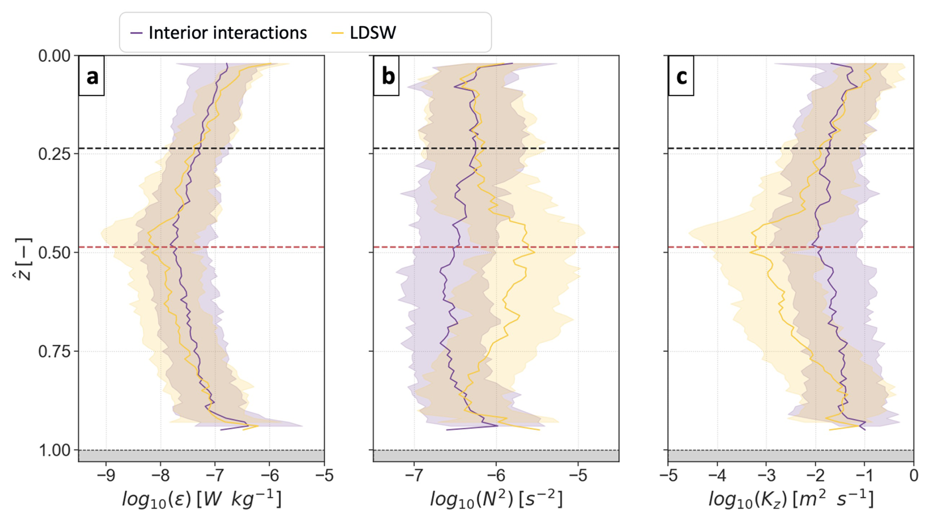
Figure 6 Average profiles with normalised depth ($\widehat{z}$) of observations of (a) dissipation rates, (b) buoyancy frequency squared, and (c) canonical diffusivity during interior interactions (purple) and low-density surface water (LDSW, yellow) periods (see Fig. 4a). In all panels, dark lines indicate the log averages, and the lighter envelopes show ±1 standard deviation. The mean surface (SML) and bottom (BML) mixed layer depths are indicated with black and red dashed lines, respectively.

The mixed layers overlapped during periods of elevated tidal and wind forcing, destabilising the variable interior stratification (Table 2). Sustained wind speeds ranging from 9–14 m s⁻¹ combined with fast flow speeds in −0.8–1.2 m s⁻¹ during episodes (iii, vi–vii). Episodes (iii, vi) also occurred during enhanced bottom shear periods, reaching $\mathrm{3.9}\times {\mathrm{10}}^{-\mathrm{6}}{\mathrm{s}}^{-\mathrm{2}}$ (see Sect. 3.1). Although boundary forcing conditions and full enhancement of water depth diffusivity were found to be similar during episodes (iii, vi–vii), the preceding stratification configurations differed significantly (Fig. 4). The depth of the SML was ∼40 m before episode (iii), compared to 80–100 m before episodes (vi–vii). BML depth extended to 30–50 m above the seabed before episodes (iii, vi), compared to ∼100 m before episode (vii). Furthermore, while the interior stratification was mostly elevated–strong ($N^{\mathrm{2}}>{\mathrm{10}}^{-\mathrm{6}}{\mathrm{s}}^{-\mathrm{2}}$) prior to episodes (iii) and (vi), it was moderate–weak before episode (vii).

Interior turbulence interactions outside mixed layer overlapping episodes were also observed (Table 2). During episodes (i–ii, iv–v, viii–x), dissipation increased to 100–1000×ϵ_p throughout the water depth, similarly to mixed layer overlapping, with an interior layer thickness reduced by approximately 3-fold from the mean. Stratification was slightly stronger than during overlapping mixed layer episodes (iii, vi–vii), leading to 3–4 orders of magnitude increase in interior K_z compared to 4–5. This notably led to mixed layer overlapping during episode (iii) but not episode (ii), where similar flow and wind speeds were found. In general, flow speeds were slower during episodes (i–ii, iv–v, viii–x), and wind speeds ranged from 2–15 m s⁻¹.

Interior turbulence interactions, including mixed layer overlapping, enhanced vertical diffusivity 20–30-fold, on average, from the baseline configuration where low-density surface water isolates bottom and surface turbulence (Fig. 6). To quantify the bulk impact of interior turbulence interactions, profiles of ϵ, N², and K_z over a period of four tidal cycles are averaged in two subsets: during or outside of the baseline low-density surface water (LDSW hereafter) configuration (see Fig. 4a). The latter includes episodes (ii–vii) of interior turbulence interactions, containing the three mixed layers overlapping episodes (iii, vi, and vii). For $\mathrm{0.25}<\widehat{z}<\mathrm{0.8}$, LDSW ϵ was 2-fold weaker, N² 4-fold stronger, and K_z 7-fold weaker. The largest difference was found at the mean interface depth of BML and interior layer ($\mathrm{0.45}<\widehat{z}<\mathrm{0.55}$), with a 20–30-fold increase in K_z during episodes of interior turbulence interactions and mixed layer overlapping (Fig. 6). Across ±30 m around the mean depth of the interior layer base ($\widehat{z}=\mathrm{0.485}$), diapycnal diffusivity averaged (log-averaged) 0.12 (0.07) and 0.04 (0.01) m² s⁻¹ for interior interactions and LDSW episodes, respectively.

The canonical diapycnal diffusivity, K_z(Γ=0.2), results from high-turbulence generated primarily in the mixed layers and is discussed in the framework of boundary limitation of overturning scales and parameterisation of diapycnal diffusivity, K_z(Γ=f(Re_b)), in Sect. 4.2. The implications for biophysical processes in the coastal ocean of K_z modulation when boundary layer turbulence overcomes transient stratification and overlaps in the interior are discussed in Sect. 4.4.

3.4 Comparison with modelled turbulence

The vertical structure of ϵ in Te-Moana-o-Raukawa / Cook Strait was primarily modulated by three external factors: winds, tides, and transient stratification. To evaluate the interaction of turbulent kinetic energy mechanisms that generate the observed ϵ structure, observations were compared to one-dimensional turbulence modelling outputs. GOTM was prescribed with simplified but realistic boundary forcing (wind stress time series and monochromatic M₂ tides; Sect. 2.4) and transient stratification (relaxation to T–S observations; Sect. 2.4). The vertical temperature structure was prescribed from glider observations, and GOTM was used to understand the interior interactions and changes in turbulent kinetic energy structure.

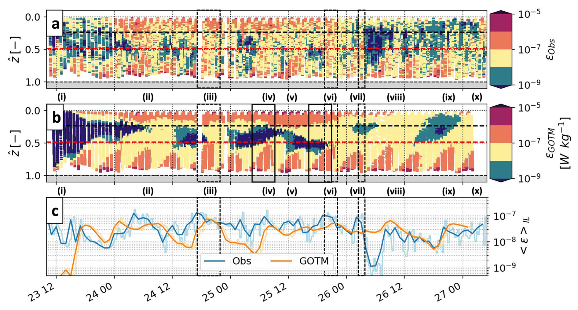
Figure 7 Normalised depth–time series of dissipation rates from (a) microstructure observations (ϵ_Obs), (b) GOTM estimates interpolated on the microstructure profile depths (ϵ_GOTM), and (c) depth averages over the mean interior layer extent (〈ϵ〉_IL) of observations (blue) compared to GOTM estimates (orange). In panels (a) and (b), the mean surface (SML) and bottom (BML) mixed layer depths are indicated with black and red dashed lines, respectively. For all panels, episodes of interior turbulence interactions are numbered (i–x), and the instances when mixed layers overlap episodes are marked with black dashed rectangles. The two solid black rectangles in panel (b) highlight case 1 (isolated boundary turbulence) and case 2 (interacting boundary turbulence) time periods used in Sect. 4.3.

GOTM captured key aspects of the magnitude, vertical structure, and interior interactions of ϵ observations (Fig. 7). Modelled surface dissipation was within an order of magnitude of observations, except during weak wind forcing when systematic overestimation was found (e.g. 23 June, Fig. 7a and b). Modelled bottom dissipation was also within an order of magnitude of observations, with the largest differences near the seabed in the intervals between enhanced ϵ pulses. The vertical ϵ structure in the mixed layers was well represented in the model, although vertical ϵ propagation away from the boundaries was largely underestimated. In general, the frequency of interior turbulence interactions was underestimated in GOTM, although interior magnitudes were reasonably represented (Fig. 7c). Interior turbulence interactions (e.g. episode ii) and boundary layer overlapping (e.g. episodes iii, vi) were too slowly established in the model, or not at all (e.g. episodes iv–v, ix), when the vertical extent of enhanced dissipation near the surface (e.g. episodes ii, iii) or the bottom (e.g. episodes iii–v, ix) was underestimated in the model.

4 Discussion

Autonomous glider observations of turbulence in a weakly stratified, energetic coastal sea captured the interactions and overlap of surface and bottom mixed layers. During a 4 d high-wind and spring-tide period, diffusivity within the respective mixed layers was enhanced. There were 10 interior turbulence interactions, including three occurrences when the mixed layers overlapped, and interior diapycnal diffusivity intensified 20–30-fold. In Sect. 4.1, we discuss the turbulence processes at play in the mixed layers and why they overlap. In Sect. 4.2, we discuss the sensitivity of the overlap observations to methodological choices. In Sect. 4.3, we discuss the sources and sinks of turbulence and their relation to the overlapping process. In Sect. 4.4, we discuss the potential implications for coastal seas mixing dynamics.

4.1 Turbulence in the mixed layers

In the BML, ϵ was highest, with log-averaged values of $\mathit{ϵ}=\mathrm{2.2}\times {\mathrm{10}}^{-\mathrm{7}}\mathrm{W}{\mathrm{kg}}^{-\mathrm{1}}$ closest to the seabed. Bottom dissipation coincided with periods of enhanced vertical shear (Fig. 8a and c). Weaker ϵ in the upper BML was an order of magnitude smaller, and, in general, dissipation in the BML was inversely related to vertical shear. On average, ϵ levels in the upper BML ($\mathrm{0.5}<\widehat{z}<\mathrm{0.6}$) were weaker during maximum than minimum shear periods but increase by an order of magnitude to $\mathit{ϵ}=\mathrm{2.2}\times {\mathrm{10}}^{-\mathrm{7}}\mathrm{W}{\mathrm{kg}}^{-\mathrm{1}}$ (3.4 times higher than for the minimum shear periods) closest to the seabed.

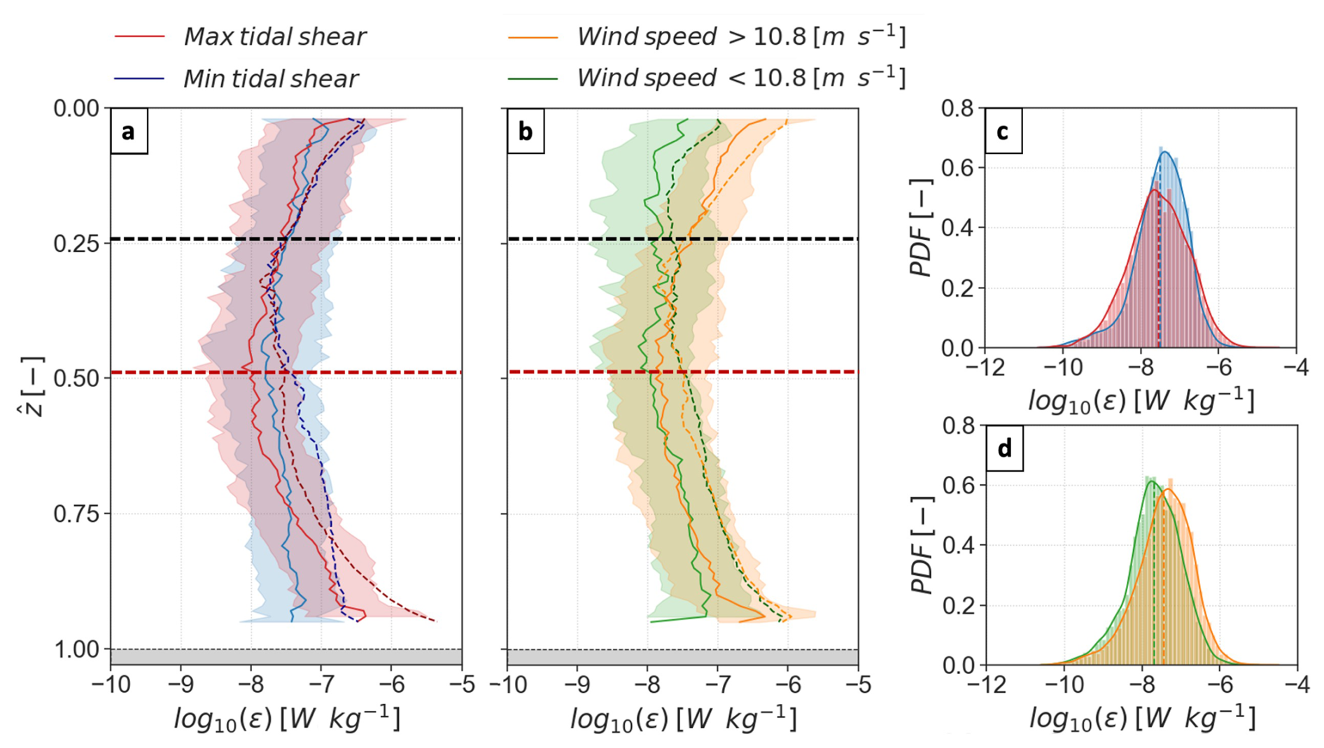
Figure 8 The vertical structure of dissipation rates during periods of varying tidal shear and wind speeds is presented here and used to validate GOTM results. Log-averaged profiles along normalised depth ($\widehat{z}$) of dissipation rates from the observations (light-coloured continuous lines, with ±1 log-standard deviation interval shaded) and GOTM estimates (dark-coloured dashed lines) for regimes of (a) maximal (red) or minimal (blue) tidal shear, and (b) high (orange) and low (green) winds (see Sect. 3.1 and Fig. 4a). Associated probability density function (PDF) of each tidal-shear and wind averaging periods of observed ϵ are shown in (c), and (d), respectively. In panels (a, b), the mean surface (SML) and bottom (BML) mixed layer depths are indicated with black and red dashed lines, respectively.

The presence of four bottom-generated ϵ pulses daily is typical at sites where M₂ barotropic tides control turbulence generation (Wang et al., 2014; Schultze et al., 2017; Becherer et al., 2022). Enhanced ϵ propagated upward to ∼80 m above the seabed in 4–4.5 h yielding an approximate vertical speed of $\mathrm{5}\times {\mathrm{10}}^{-\mathrm{3}}\mathrm{m}{\mathrm{s}}^{-\mathrm{1}}$ (see e.g. episodes v, viii in Fig. 4), of the same order of magnitude as ϵ observations driven by $\sim \mathrm{1}\mathrm{m}{\mathrm{s}}^{-\mathrm{1}}$ tidal forcing in a weakly stratified shelf sea (Thorpe et al., 2008). The ϵ envelope for a pulse generated close to the wall during the acceleration phase reached its maximal height above the bottom after 4–4.5 h of the deceleration phase. Large-eddy simulations of oscillatory current-driven turbulence in a stratified boundary layer (Gayen et al., 2010) match the ϵ dynamics of tidal phases in Cook Strait. Stratification adjacent to the bottom mixed layer modulated the upward extension of bottom-generated turbulence, akin to observations (Wang et al., 2014) and simulations (Gayen et al., 2010) elsewhere.

Strong winds elevated dissipation in the SML (Fig. 8b and d), and the ϵ log-mean increased up to 20-fold from the low wind conditions. Elevated winds did not always induce overlapping mixed layers; however, ϵ in the interior layer increased 2-fold compared to low wind conditions. The depth and magnitude to which ϵ was enhanced are consistent with high-wind-driven mixing in shelf seas of various depth ranges (MacKinnon and Gregg, 2005; Williams et al., 2013; Schultze et al., 2020).

When the SML and BML overlapped, interior ϵ increased by 3 orders of magnitude from the ϵ_p baseline (Table 2). Mid-water depth log averages were 4 times greater than during the more strongly stratified LDSW conditions (Fig. 6). Generally, interior ϵ was of the same order of magnitude (or less) as the near-boundary levels (Fig. 4d). This was also true during SML and BML overlapping, suggesting that, in these Te-Moana-o-Raukawa / Cook Strait observations, boundary-generated turbulence combined linearly in the interior. This might indicate that the boundary-generated turbulence, although originating from non-linear sources, can appear as a linear response of the mean shear flow (Landahl, 1988, 1989; Jiménez, 2013). As such, the observations did not show that boundary-generated turbulence interacted with interior stratification to produce turbulence via internal wave generation and breaking (Gayen et al., 2010; Zhang and Tian, 2014; Wang et al., 2014).

An interior region of approximately ∼50 m had moderate–elevated ϵ in the 2 h preceding the mixed layer overlapping episode (vi) (Fig. 4d). This notable occurrence appeared to be linked to a detached burst of turbulence from the strong BML pulse of episode (v), rising at 2–5 m s⁻¹. With a certain degree of vertical spreading, it is akin to the BML burst ejection mechanism described in Thorpe et al. (2008). Albeit of weaker ϵ, this pattern of burst ejection outside of the BML was observed two more times. All three occurrences happened during particularly deep and strong stratification configurations in the water column. If the bulk interior stratified layer sits within the bulge of high turbulence tidal pulses, a portion of the bottom-generated turbulence can be suppressed, and high-ϵ bursts can detach and travel upward in the water column (Thorpe et al., 2008). Similar ejection mechanisms can affect sediment transport processes in bottom boundary layers (Li et al., 2022; Wu et al., 2022).

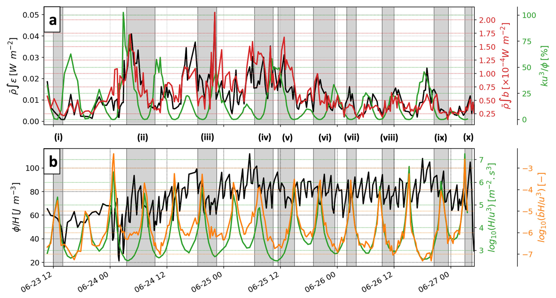
Figure 9 Depth-integrated metrics provide background to events of interior turbulence interactions and mixed layer overlapping. (a) Observed depth-integrated dissipation rates and buoyancy flux (b; see Fig. A2a), contextualised with a simple model for the proportion of work needed to mix the water column attributed to tidal kinetic energy ($k{u}^{\mathrm{3}}/\mathit{\varphi }$, see details in text). (b) Observed work required to mix the water column ($\mathit{\varphi }/H$, also called potential energy deficit) contextualised with the Simpson–Hunter model for stratification ($H/u^{\mathrm{3}}$) and the non-dimensional contribution of mean surface buoyancy flux to bulk stratification ($\overline{b}H/u^{\mathrm{3}}$, with $\overline{b}$ denoting the 0–50 m average). Episodes of interior turbulence interactions are highlighted with light grey rectangles and numbered (i–x).

The two main overlapping episodes (iii) and (vi) were of similar duration, forcing speeds, and turbulence characteristics (Table 2); however, initial conditions were different (Fig. 4). In the 2–3 h prior to either episode, surface and bottom-driven elevated–strong ϵ were co-located in time with a thick (>50 m) and elevated–strong interior stratification (Fig. 4c and d). In both cases, the BML depth was relatively deep, within 50 m of the seabed. The SML depth was approximately twice as thick before (vi), but the enhanced surface ϵ extended deeper ahead of the mixed layer overlapping episode (iii). Similar strength in stratification occurred near the seabed, but the bottom-driven turbulence of episode (iii) appeared to be strong enough to destabilise stratification and connect with surface-driven ϵ during the decelerating tidal phase. This is different from episode (vi), which is characterised by a more distinctive BML ϵ pulse. For this episode, the overlapping mechanism was initiated by turbulence present in the mid-water column, most likely a burst ejected from the BML during episode (v) (Thorpe et al., 2008).

Interior turbulence interactions were also identified in the results, representing mixing-layer overlapping (see Sect. 3.3 and Fig. A1). Mixing layers portray active mixing, referring to a different timescale than the mixed layer, which illustrates the history of mixing (Sutherland et al., 2014; Giunta and Ward, 2022). Periods when mixing layers overlap but mixed layers do not (events i–ii, vi–v, viii–x) thus indicate vigorous mixing activity and enhanced vertical turbulence exchanges (see Sect. 4.3) that fail to bring interior tracers, e.g. here temperature, to homogeneity. Differences between mixed- and mixing-layer overlapping attest to the myriad of dynamical surface- and bottom boundary layer processes that affect turbulence generation and the stratification it works against, e.g. surface-driven restratification allowing for a shallower SML than surface mixing layer (Sutherland et al., 2014; Esters et al., 2018).

The presence of mixed layer overlapping events was compared to bulk metrics for stratified systems (Fig. 9). For a depth-integrated metric, the pulses of dissipation enhancement generally match well-mixed conditions, where ${\log }_{\mathrm{10}}(H/u^{\mathrm{3}})$, the Simpson–Hunter stratification index, is below the commonly used 2.7–3 critical range (Simpson and Hunter, 1974; Marsh et al., 2015; Timko et al., 2019). Applying the bulk formulation of a Cook Strait stratification study by Bowman et al. (1983), depth-integrated ϵ variations match conditions where the majority of the work to mix the water column ($\mathit{\varphi }/H$, potential energy deficit per unit volume) would be attributed to tidal kinetic energy dissipation (Fig. 9a). The short-lived nature of mixed layer overlapping is difficult to distinguish using bulk metrics. For example, events (vi–vii) were not associated with high tidal energy dissipation ($k{u}^{\mathrm{3}}/\mathit{\varphi }<\mathrm{30}\mathrm{\%}$) before or during the events. The contribution of surface buoyancy fluxes to bulk stratification ($\overline{b}H/u^{\mathrm{3}}$) can be noted only before and during events (ii–vi), indicating only a minor contribution to restratification processes (Fig. 9b). While broadly, some of the turbulence and mixed layer overlapping characteristics can be resolved by variations in these bulk metrics, much more complexity is at play when mixed boundary layers overlap.

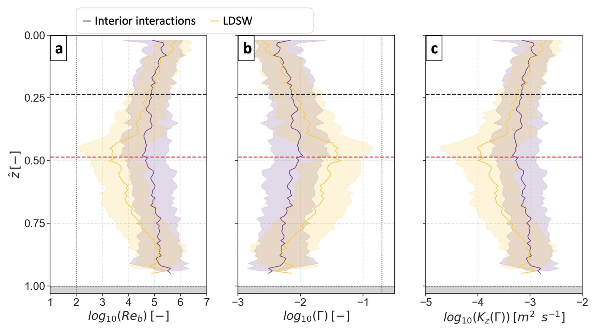
Figure 10 Elevated levels of turbulence activity lead to parameterised mixing efficiency and diapycnal diffusivity reduced a hundredfold compared to canonical values. Average profiles with normalised depth ($\widehat{z}$) of observations of (a) buoyancy Reynolds number, (b) mixing efficiency coefficient, and (c) diffusivity with a variable mixing efficiency coefficient, during interior interactions (purple) and low-density surface water (LDSW, yellow) periods (see Fig. 4a). In all panels, dark lines indicate the log averages, and the lighter envelopes show ±1 standard deviation. The mean surface (SML) and bottom (BML) mixed layer depths are indicated with black and red dashed lines, respectively. In panels (a, b), the dotted black vertical lines indicate the Re_b=100 threshold for isotropic turbulent motions, and the canonical Γ=0.2 value for mixing efficiency, respectively.

4.2 Sensitivity to stratified turbulence observing methods

Estimating background stratification, N², remains a source of uncertainty for the application of Eq. (1), the Osborn formula (Gregg et al., 2018; Arthur et al., 2017). In the observations, adiabatically rearranged (i.e. sorted) vertical density profiles were used to compute a statically stable background stratification, i.e. N²>0 (Thorpe and Deacon, 1977; Mater et al., 2015). In the GOTM simulations, N² is computed internally using the prescribed, raw, glider-based T and S profiles (see Sect. 2.4). Convective adjustment subroutines are used in GOTM to control static stability; however, N²<0 is allowed (Umlauf et al., 2012).

Positive values of the buoyancy flux, G, were output by GOTM because raw, un-sorted temperature and salinity observations were prescribed to the model (see further discussion of model sensitivity to observation interpolation in Sect. 4.3). Albeit of secondary importance relative to shear production, G>0 values can be of similar magnitude to T_k in some portions of the boundary layers (Fig. 11 and A3). Sign-indefinite G represents the reversibility of potential and kinetic energy exchanges during turbulent mixing episodes, identified as a source of uncertainty when quantifying irreversible mixing processes (Caulfield, 2020). Thus, using adiabatically rearranged density could lead to some overestimation of the proportion of TKE dissipation that drives irreversible mixing and enhances diapycnal diffusivity (Eq. 1).

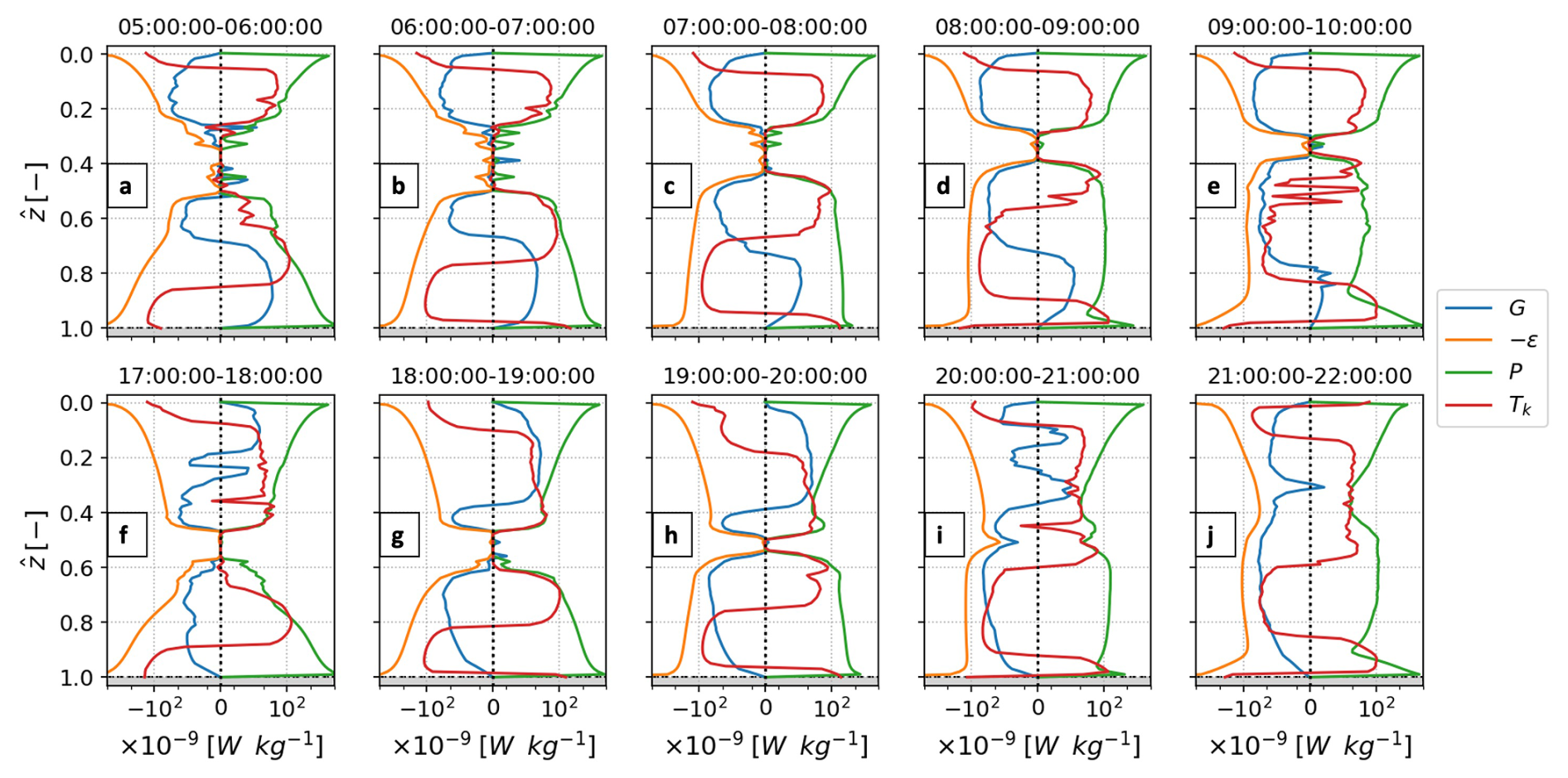
Figure 11 Shear-driven turbulent kinetic energy, produced near the boundaries, can interact in the interior when vertical transport is enhanced. Normalised hourly averaged profiles of GOTM estimates of TKE source (>0) and sink (<0) terms of Eq. (3) for (a–e) (case 1) isolated or (f–j) (case 2) interacting, turbulent layers. Buoyancy flux (blue), dissipation rate (orange), shear production (green), and vertical transport (red) of TKE are shown. The continuous and dashed lines for −ϵ represent where ϵ is higher or lower than ϵ_p, respectively.

The use of a constant mixing efficiency coefficient, i.e. Γ=0.2, potentially overestimates diapycnal diffusivity of weakly stratified and energetic turbulence (Bluteau et al., 2017; Monismith et al., 2018). This is especially relevant to homogeneous, shear-driven turbulence, such as is expected in strongly forced boundary layer flows, where boundary proximity can limit the growth of turbulent eddies (Shih et al., 2005; Holleman et al., 2016; Monismith et al., 2018). Due to the elevated boundary-driven turbulence observed in Te-Moana-o-Raukawa / Cook Strait, differences between using Γ=0.2 or a buoyancy Reynolds number-based parameterisation to quantify diapycnal diffusivity are evaluated. The Bouffard and Boegman (2013) parameterisation is used here, supported by a range of modelling, field, and laboratory measurements of high-turbulence Γ (Barry et al., 2001; Shih et al., 2005; Monismith et al., 2018). For the complete time series, the mean diffusivity for parameterised K_z was $\mathrm{9}\times {\mathrm{10}}^{-\mathrm{4}}{\mathrm{m}}^{\mathrm{2}}{\mathrm{s}}^{-\mathrm{1}}$, while the mean canonical K_z was 0.1 m² s⁻¹. As such, the bulk difference was of 2 orders of magnitude, with the mean parameterised K_z being 0.9 % of the canonical K_z. Further, the variable Γ modulates the overall K_z structure through the SML and BML. Parameterised log-mean Γ values can be up to 60 times reduced from 0.2 near the boundaries, and up to 20- and 4-fold at the mean interior layer base ($\mathrm{0.45}<\widehat{z}<\mathrm{0.5}$) during LDSW and interior turbulence interactions episodes, respectively. This led to a 5-fold increase in K_z(Γ) during interior turbulence interactions episodes, compared to 20–30-fold for K_z(Γ=0.2) (Fig. 6). In the ±30 m around $\widehat{z}=\mathrm{0.48}$, the mean interior layer base, mean (log mean) K_z(Γ) levels are $\mathrm{5}\times {\mathrm{10}}^{-\mathrm{4}}$ ($\mathrm{3}\times {\mathrm{10}}^{-\mathrm{4}}$) and 10⁻³ ($\mathrm{1.1}\times {\mathrm{10}}^{-\mathrm{3}}$) m² s⁻¹ for interior turbulence interactions and LDSW episodes, respectively. Interior turbulence interactions enhance mean (log-mean) diffusivity by 2-fold (3-fold), compared to 3-fold (7-fold) for K_z(Γ=0.2) at the interior mixed layer boundaries (Fig. 6). At the interior mixed layer boundary, mean parameterised K_z was elevated to $\mathrm{1}\times {\mathrm{10}}^{-\mathrm{4}}{\mathrm{m}}^{\mathrm{2}}{\mathrm{s}}^{-\mathrm{1}}$ during overlapping, only 0.5 % of the corresponding mean K_z(Γ=0.2). Using an arguably more realistic scaling for Γ, interior turbulence interactions, including mixed layer overlapping, enhance diapycnal diffusivity, albeit at weaker K_z than when using a constant coefficient.

4.3 Sources and sinks of interior turbulence

Understanding the mechanisms that led to isolated (case 1) or interacting boundary-driven turbulence (case 2) was examined using GOTM-based hourly averages of TKE source (>0) and sink (<0) terms of Eq. (3) (Fig. 11). The turbulent boundary layers were defined using the same threshold criteria that were applied to OMG observations to detect interior turbulence interactions, analogous to mixing-layer overlapping (Sect. 2.2; see also Fig. A1). In both cases, turbulent boundary layers, where shear production and dissipation are the dominant source and sink of TKE, respectively, grow through entrainment against the stabilising interior stratification that inhibits vertical turbulent exchanges (Gayen et al., 2010; Yan et al., 2022).

Case 1 and 2 are initially forced by similar wind strength (in 10–15 m s⁻¹) and tidal flows, but differ in upper water column stratification and turbulent surface layer extent (Figs. 2, 4c). Both cases showed similar depth extent of bottom turbulence, but surface turbulence extended deeper for case 2 (see Fig. 11a and f). In both cases, “vertical transport” T_k is a near-boundary TKE sink of secondary importance (1–2 orders of magnitude lower than ϵ) and a primary TKE source (comparable magnitude to P) in the turbulent boundary layers. Kinetic energy transfer from the boundaries towards the interior was confined in the respective turbulent layers, since T_k→0 in the interior (Yan et al., 2022; Becherer et al., 2022).

During subsequent stages, when the wind forcing remains strong and the tidal forcing enters the deceleration phase, the turbulent bottom layer grows in both cases, but the turbulent surface layer only significantly deepens in the interacting boundary-driven turbulence scenario of case 2 (Fig. 11b–e, g, and h). The shallow transient stratification of case 1 was strong enough to dampen T_k and impede surface layer growth, isolating the turbulent layers. The turbulent layers remain isolated, even though high source levels (primarily P and T_k) are observed in the bottom layer and especially, in the deep edge of the interior separation (Fig. 11b–e).

In case 2, high levels of T_k (comparable to P) at both edges of the interior separation successfully provide the TKE source that supports the gradual pycnocline erosion from above and below (Yan et al., 2022; Becherer et al., 2022) during a transition phase (Fig. 11g and h), until the layers overlap (Fig. 11i and j). T_k fully connects in the interior when turbulent layers fully overlap, due to the slow reduction of interior stratification rather than boundary layer growth, as suggested in Yan et al. (2022). T_k further represents the vertical divergence of the TKE flux, which is a significant source of deviation from local TKE balance (Scully et al., 2011). Whether T_k directly contributes to stratification erosion or contributes indirectly to dissipation-driven mixing was not ascertained here. Nevertheless, this process appears to dominate. Six out of the 10 interior turbulence interaction events, including the three overlapping the mixed layer (ML), show similar T_k structure and interplay of TKE terms (Fig. A3). T_k in the interior, also near the boundaries, is in places of comparable magnitude to local shear production, as another phase of enhanced tidal shear starts and wind fluctuates (Fig. 2). Overall, dissipation is driven up by two orders of magnitude in the mid-water column.

The primary difference between cases 1 and 2 is in the initial turbulent surface layer extent, a balance of wind-driven turbulence against interior stratification for the examples chosen here. In 𝒪(200 m) deep, tidally forced systems, turbulent boundary layer overlapping occurs when winds are high enough and interior stratification fluctuates, echoing the insights of Yan et al. (2022), where Langmuir super-cell turbulence is theorised to drive boundary layer overlapping, albeit in much shallower systems.

The buoyancy flux (G) is a TKE sink for most of the water column for both cases, but a source near the surface (case 2) or the bottom (case 1) boundary. Although of negligible magnitude against primary TKE terms in Eq. (3), intermittent G>0 spikes are of comparable amplitude to P spikes found in the interior during the initial stage of case 1 (see Fig. 11a and b). The contribution of buoyancy fluxes to turbulence production thus appears non-essential to the overlapping process. It contributed, however, to the interior turbulence interactions of event (viii), as G was above ${\mathrm{10}}^{-\mathrm{9}}\mathrm{W}{\mathrm{kg}}^{-\mathrm{1}}$ across the water depth (Fig. A3d). Notably, further processing of observation interpolation (e.g. sorting T–S observations and increasing the relaxation timescale) reduces G>0 occurrences and magnitude (not shown). These adjustments, however, cause a significant deviation of the other TKE terms from the GOTM results presented here, which best portray the direct OMG observations of ϵ structure and boundary layer interactions.

Winds and tides consistently shape the vertical structure of dissipation in the GOTM regime averages (Fig. 8). While the ϵ structure of enhanced boundary forcing in GOTM broadly matched observations, the depth away from boundary of log-mean ϵ increased during periods of enhanced tidal shear (Fig. 8a) or wind speed (Fig. 8b) was underestimated in the model. As a consequence, several episodes of interior turbulence interactions in the observations were misrepresented in the GOTM results. For example, in Fig. 7, mean levels of the interior layer ϵ were underestimated (for example, episodes iv and vii) or overestimated (for example, episodes viii and ix). The former could originate in the underestimation of either surface (iv) or bottom (vii) turbulence transfer to the interior, while the latter could be an indication of lateral transport of turbulence.

4.4 Implications of overlapping boundary layers in coastal seas

Varying stratification and forcing in shelf seas compete to enable interior turbulence interactions and enhanced diffusivity. Although Te-Moana-o-Raukawa / Cook Strait has been classified as weakly stratified (Stevens, 2014, 2018), in this study, transient stratification opposed interior turbulence interactions and mixed layer overlapping, with a bulk order-of-magnitude difference (Fig. 6). Further, bulk stratification, ${\log }_{\mathrm{10}}(H/u^{\mathrm{3}})$, ranged from 2.3–7.4 s³ m⁻² (Fig. 9b), consistently with, if not more strongly stratified than other Te-Moana-o-Raukawa / Cook Strait studies (Bowman et al., 1983) and shelf seas of similar depths (Garrett et al., 1978; Marsh et al., 2015). Restratifying surface buoyancy fluxes, scaled to bulk stratification ${\log }_{\mathrm{10}}(\overline{b}H/u^{\mathrm{3}})$, averaged −4.3, suggesting a similar influence to that in much shallower estuarine systems (Ralston et al., 2010; Orton et al., 2010). This indicates that if it were not for the transient stratification influx at the base of the warm surface waters, from water masses advected through the strait, and to a minor extent, restratification from buoyancy fluxes, interior turbulence interactions and full-water column turbulence would have occurred at tidal frequency, during the high-winds period.

Horizontal variability at submesoscales in Greater Te Moana-o-Raukawa / Cook Strait influences transient stratification. Evidence of a SST front advected ∼40 km south during 25–27 June is shown here (Fig. 3). At the submesoscale in Greater Te Moana-o-Raukawa / Cook Strait, SML baroclinic instabilities and fronts of typical length scale 0.1–1.6 km can have an advection timescale of 0.2–8 h (Jhugroo et al., 2020), comparable to the 6 h period of tidal generation of BML in a strait. These features have been shown to strengthen vertical stratification to $\mathcal{O}\left({\mathrm{10}}^{-\mathrm{4}}{\mathrm{s}}^{-\mathrm{2}}\right)$, reduce mixed layer depth, and decrease diapycnal diffusivity (Jhugroo et al., 2020). Moreover, the interaction of surface momentum fluxes and horizontal gradients can affect advection patterns in Greater Te-Moana-o-Raukawa / Cook Strait (Jhugroo et al., 2020) and wind-driven turbulence through wind straining in broadly similar systems (Verspecht et al., 2009).

Understanding the balance of processes when boundary-driven turbulence interacts in the interior and mixed layers eventually overlap is an important, new component of coastal ocean productivity. During mixed layer overlapping, the water column becomes well mixed, suggesting fully homogeneous phytoplankton distributions (Becherer et al., 2022). For periods when surface and bottom mixed layers remain isolated, enhanced turbulence can still modify diapycnal diffusivity at the boundary edges of a weakly to moderately stratified interior layer. Antecedent conditions determine whether the interior layer is maintained or eroded during intensified turbulence episodes, which have implications for biological production in the interior and below the surface mixed layer.

5 Conclusions

Here we present a sizable dataset of 𝒪(43 000) measurements of elevated turbulence from an ocean glider, using a new electromagnetic sensor technology to refine glider speed measurements. This work showcases the value of autonomous sampling platforms for capturing intermittent mixing processes and characterising the vertical structure of mixing in shelf seas. Boundary-driven turbulence interacted in the interior and mixed layers overlapped, under moderate–strong wind and tide forcing, during 35 % of a 4 d period in a 𝒪(200 m) deep system. These observations are novel and show that the set of ocean conditions that allow for overlapping is more frequent than previously observed and can occur in deeper shelf seas. As revealed by continuous sampling, the interplay of boundary-driven turbulence regulates diffusivity in the coastal ocean interior, potentially influencing primary productivity and air–sea fluxes. Limits for both numerical and field-based stratified turbulence studies were discussed and, optimistically, will encourage further exploration of energetic turbulence in coastal seas.

Appendix A: additional information on the process of boundary layer overlapping

A1 Interior turbulence interactions and mixing layers

Figure A1 shows the same panels as Fig. 4c and d, i.e. buoyancy frequency squared N² (Fig. A1a) and dissipation rates ϵ (Fig. A1b). Figure A1a is identical to Fig. 4c, with surface (SML) and bottom (BML) mixed layer depths highlighted. As described in Sect. 2.2 of the main text, the depths of the mixed layers are calculated using a threshold Δθ=0.05 °C. Figure A1b, however, highlights surface and bottom mixing-layer depths. The depths of the mixing layers are calculated using the standard approach of smoothing the ϵ profiles and using the ${\mathit{ϵ}}_p=\mathrm{3}\times {\mathrm{10}}^{-\mathrm{9}}\mathrm{W}{\mathrm{kg}}^{-\mathrm{1}}$ threshold (Sutherland et al., 2014; Esters et al., 2018; Giunta and Ward, 2022), also used to detect the duration of the events of interior turbulence interaction events (i–x). The figure illustrates the physical significance of the interior turbulence interaction events, representing mixing-layer overlapping, occasionally escalating to mixed-layer overlapping (events iii, vi–vii).

A2 Buoyancy fluxes and restratification

Figure A2 shows buoyancy flux (b=K_zN²) estimates from Ocean Microstructure Glider (OMG) measurements, using two different formulations for diapycnal diffusivity ($K_z=\mathrm{\Gamma }\mathit{ϵ}/N^{\mathrm{2}}$) (Osborn, 1980). Figure A2a shows b^BB, the buoyancy flux using the Bouffard and Boegman (2013) formulation for K_z and Γ. Figure A2b shows b^O, the buoyancy flux using the canonical Γ=0.2 parameterisation from Osborn (1980). Canonical b^O is only shown for comparison, as its variability is by construction equal to that of ϵ, i.e. $b^{\mathrm{O}}=K_z(\mathrm{\Gamma }=\mathrm{0.2})\times N^{\mathrm{2}}=\mathrm{0.2}\times \mathit{ϵ}$. Figure A1a supports the observation of a negligible contribution of buoyancy fluxes to restratification processes. Buoyancy fluxes potentially play a role, however, in providing strengthened stratification to oppose overlapping, e.g. just before event (ii), where the conditions for mixed layer overlapping are gathered, but the interior stratification holds (Fig. A2a). Figure A2a further provides context for depth-integrated and depth-averaged results presented in Fig. 9.

A3 Turbulence budget

Figure A3 shows the turbulent kinetic energy (tke, k) balance terms computed using the General Ocean Turbulence Model (GOTM). The figure is provided to support a number of observations made in Sect. 4.3. Specifically, the influence of turbulent transport T_k on the process of interior turbulence interactions and eventual mixed layer overlapping is supported. Six of the 10 events (ii–iii, vi–ix) show enhanced T_k transporting boundary-generated turbulence, eroding interior stratification, and connecting across the interior. Events (iii, vi–vii) clearly reflect this pattern, supporting its influence on breaking interior stratification and allowing mixed layers to dramatically entrain and overlap.

Figure A1 Depth–time series of (a) buoyancy frequency squared N², with surface (SML, black line) and bottom (BML, red line) mixed layer depths, respectively, and (b) dissipation rates ϵ, with surface (black line) and bottom (red line) mixing-layer depths, respectively. Mixed layer depths are computed using a temperature threshold. Mixing-layer depths are computed using a dissipation rate; see details in the text. Episodes of interior turbulence interactions are shaded and numbered (i–x).

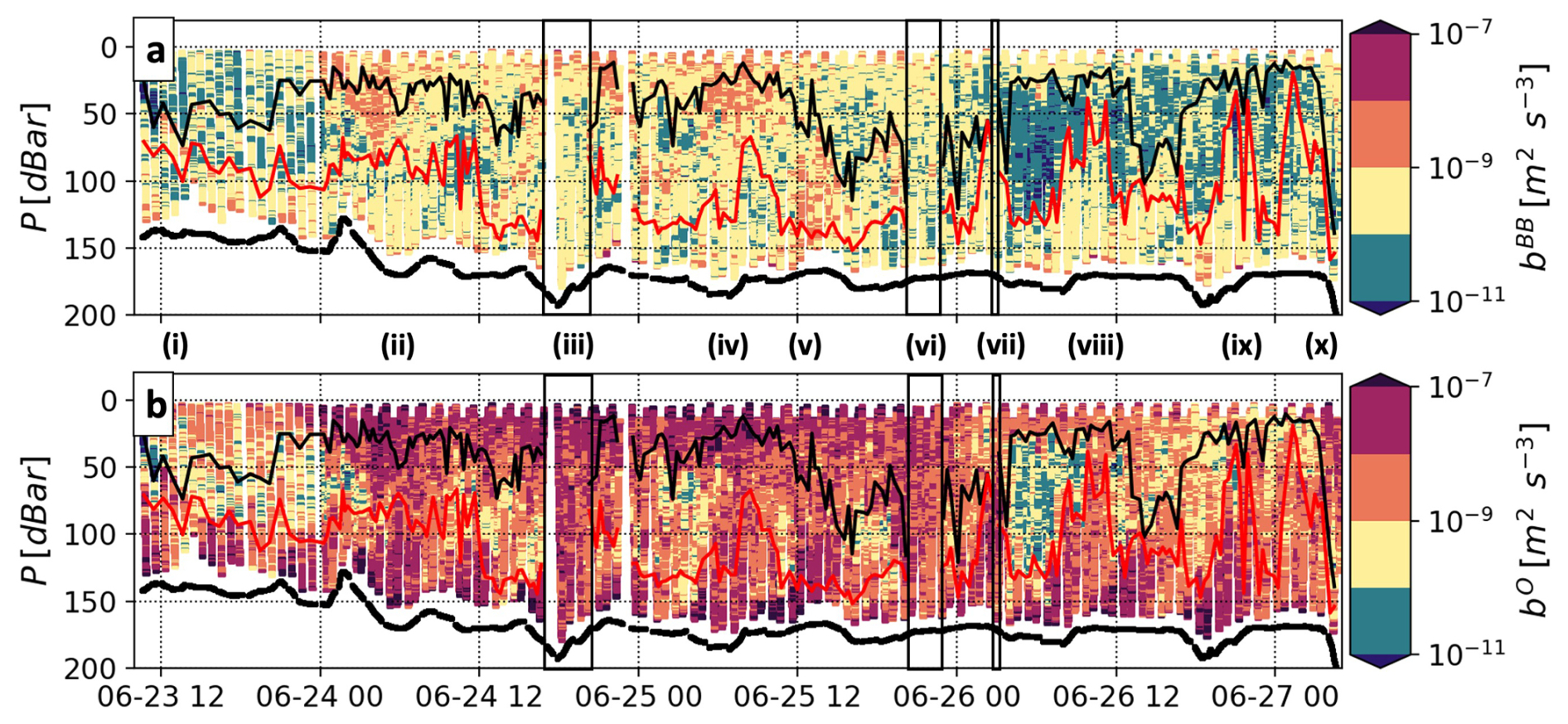
Figure A2 Depth–time series of buoyancy flux b=K_zN², using the Osborn (1980) formula for $K_z=\mathrm{\Gamma }\mathit{ϵ}/N^{\mathrm{2}}$. (a) Γ=f(Re_b) using the Bouffard and Boegman (2013) formula, labelled b^BB, and (b) Γ=0.2, labelled b^O. In both panels, the thick black dashed line is the seabed, and the surface (SML) and bottom mixed layer (BML) depths are shown with black and red lines, respectively. Episodes of interior turbulence interactions are numbered (i–x), and the instances when mixed layers overlap are marked with black dashed rectangles.

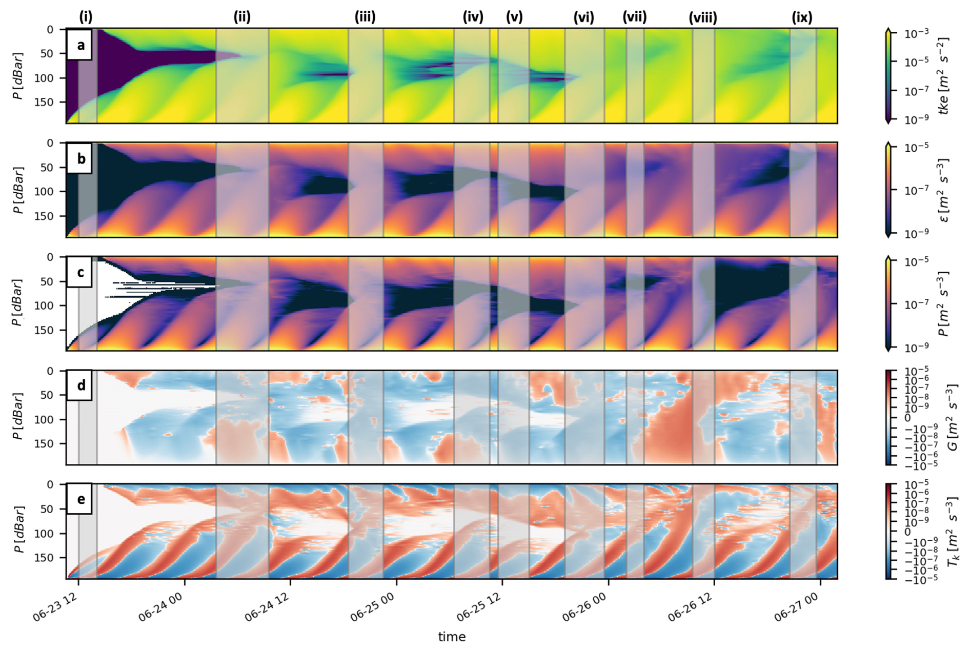
Figure A3 Depth–time series of turbulent kinetic energy (tke) balance terms from the General Ocean Turbulence Model (GOTM): (a) total tke, (b) dissipation rate ϵ, (c) shear production P, (d) buoyancy flux G, and (e) total turbulent transport T_k. Episodes of interior turbulence interactions in the OMG observations are highlighted with light grey rectangles and numbered (i–ix), and event (x) is not shown.