Coupled estimation of internal tides and turbulent motions via statistical modal decomposition

We present a data-driven modal-decomposition method that extracts the part of an incoherent internal tidal wave that correlates with the proper orthogonal decomposition (POD) of a turbulent mesoscale flow. This method exploits the a priori knowledge that the incoherent internal tide arises from interactions between an incident wave and the turbulent flow and also exploits the corresponding statistical correlation between the two types of motions. The method is presented and tested in an idealised framework based on the rotating-shallow-water model, where we provide a physical interpretation for the decomposition method based on theoretical considerations. Using idealised simulations with a plane wave propagating through a zonal turbulent jet, we first propose the use of the modal-decomposition method as a data analysis technique to understand how the wave is scattered by the flow. In a second step, we construct an estimation algorithm capable of separating the entangled contributions of the wave and mesoscale motions from a single sea surface height snapshot. This algorithm, which consists of estimating the POD coefficients of the turbulent flow shared by the wave and jet modes, is particularly suitable for configurations where the jet contribution to the sea surface height (SSH) is larger than that of the wave.

1 Introduction

Internal tides (ITs) are internal waves generated by the interaction of the barotropic tide with the irregular topography, such as ridges or continental slopes, that propagate mainly at tidal frequencies. They are ubiquitous in the ocean and play a crucial role in vertical mixing and energy transport, especially in the deep ocean (Munk and Wunsch, 1998; Vic et al., 2019). Propagating over large distances, they encounter regions with energetic mesoscale turbulence and lose their fixed-phase relationship with the astronomical forcing through non-linear interactions with this turbulence. The resulting incoherent internal-tide field (often called a “non-phase-locked” or “non-stationary” internal tide in the literature), which is highly unpredictable, complicates, for example, our ability to disentangle internal tides and low-frequency turbulent signals from satellite data (Richman et al., 2012). Due to their large coverage and overall impact on the ocean (Zaron, 2017; Nelson et al., 2019), there is a need to understand how incoherent waves propagate, which includes developing algorithms for estimating and separating the surface signature of internal tides and the mesoscale flow from observational data.

In the physical oceanography community, various studies have examined the impact of a low-frequency turbulent flow on internal waves using various methodological approaches. Ponte and Klein (2015) demonstrated, using idealised numerical experiments featuring a plane wave propagating through a zonal baroclinic jet, that the increase in the energy of the turbulent jet enhances the loss of coherence in the internal-tide field. Savva and Vanneste (2018) described, based on kinetic transport theory, how random quasi-geostrophic and barotropic flows impact energy exchanges in a scattered plane wave. Dunphy et al. (2017), Kelly et al. (2016), and Rainville and Pinkel (2006), among others, studied the propagation of ITs using reduced-order models derived from a Galerkin projection onto a basis of vertical modes. Ward and Dewar (2010) applied a multiscale analysis to the rotating-shallow-water model (RSW) to study the scattering of inertia–gravity waves (IGWs) by the low-frequency flow. The authors showed that waves that resonantly interact with the jet transfer their energy to waves of equal wavelength and that this transfer is intensified for short-wavelength and strongly turbulent flows. A consequence of the non-linear interactions between the ITs and the low-frequency flows is a spectral broadening, often referred to as “cusps” (Colosi and Munk, 2006; Zaron, 2022), which is a direct translation of the loss of coherence in the signal. Indeed, the quadratic non-linear term becomes, in time–frequency space, a convolution operator between the wave and the mesoscale fluctuations. The spectrum of coherent ITs, which corresponds to a finite Dirac sum, is thus broadened by the mesoscale flow, giving rise to an incoherent broadband spectrum. Spectral broadening is a general characteristic of scattered-wave fields, widely studied in other disciplines (e.g. in aero-acoustics; Campos, 1978; Clair and Gabard, 2016).

Recently, several methodological approaches have been developed to address the issue of the separation of ITs and balanced motions (BMs), motivated, in particular, by the launch of the SWOT mission (Fu et al., 2024). Due to the presence of an incoherent component, similar wavelengths, and a large time lag between two swaths, simple filtering or harmonic decomposition strategies are often ineffective. Some methods are based on physical approaches, such as in the study of Ponte et al. (2017), who assumed a weak signature of ITs on surface density fields and considered potential vorticity dynamics to identify the BMs from the observations. In the realm of data assimilation methods, Le Guillou et al. (2021) developed a coupled iterative approach based on a 4D-Var algorithm for ITs and back-and-forth nudging for BMs. In the range of data-driven methods, there has been a recent focus on deep-learning approaches to disentangle low- and high-frequency signals (Wang et al., 2022; Gao et al., 2024). Gao et al. (2024) address, in particular, the difficulty caused by the long revisit time of altimeters by developing a method based on single sea surface height (SSH) snapshots. In closer connection to the methodology that will be presented in this paper, Egbert and Erofeeva (2021) and Tchilibou et al. (2024) proposed methods based on a proper orthogonal decomposition (POD) of the IT sea surface height (SSH) field, computed based on a HYCOM-based realistic simulation in the case of the former and based on a filtered daily SWOT swath in the case of the latter.

In this paper, we introduce a data-driven modal decomposition of a wave field scattered by a turbulent mesoscale jet. We focus on methods based on the POD (Berkooz et al., 2003; Lumley, 1967). The POD (often called empirical orthogonal functions – EOFs – in the geophysical fluid dynamics community) is a modal-decomposition method designed to extract recurrent phenomena from flow data (Long et al., 2021). We propose two different methods, namely the broadband POD (BBPOD) and an algorithm based on the extended POD (EPOD; Boree, 2003). Both methods rely on the physical consideration that the scattering of the wave field, corresponding to the time evolution of its complex amplitude, is driven by the mesoscale dynamics and therefore occurs at a similar timescale (Bühler, 2014). With this consideration in mind, the BBPOD algorithm corresponds to a POD of the complex demodulated variables and extracts the most energetic modes of variability of a high-frequency component associated with a broadband spectrum. It shares similarities with the spectral POD algorithm (Welch, 1967; Towne et al., 2018), as will be discussed further in the paper. The second method applies the extended POD method to the complex wave amplitude in order to extract spatial modes that are correlated with the POD modes of the jet, thereby providing a decomposition of the flow that takes into account the coupling between the mesoscale dynamics and the wave.

Then, we take advantage of this EPOD-based decomposition method to build an algorithm for estimating the mesoscale dynamics and wave fields – including velocities – from a single SSH observation. In particular, we address configurations where the jet component dominates the flow, in which case the weak internal-tide signal can still be estimated by the coupling induced by their correlation. The algorithm is tested on idealised simulations of a one-layer RSW model representing such a configuration.

The structure of this paper is as follows. We begin in Sect. 2 by describing the RSW model on which this study is based. Derivation of the equations for the ansatz of the complex amplitudes is then given in order to complement the data-driven methods with a physical interpretation. In Sect. 3, the BBPOD- and EPOD-based methods are first presented (Sects. 3.1 and 3.2) before a description of the algorithm to disentangle observations (Sect. 3.3). Finally, Sect. 4 gathers the numerical results computed from five idealised simulations, including a data analysis of the variability of the wave field (Sect. 4.2), and results from the estimates of the mesoscale jet and the internal tide are given in Sect. 4.3.

2 Non-linear interactions between mesoscale turbulence and high-frequency waves

We present in this section the (dimensionless) one-layer rotating-shallow-water model (RSW), which is an adequate idealistic model to analyse non-linear interactions between high-frequency waves and a low-frequency turbulent flow (e.g. Vallis, 2006; Ward and Dewar, 2010). A set of asymptotic equations is then derived for the complex wave amplitude and the evolution of the incoherent part. We mention that, since internal tides interacting with mesoscale turbulence are the main target of this study, the waves will be often referred to as internal tides (ITs), and the low-frequency turbulent flow will be referred to as mesoscale flow throughout the paper.

2.1 One-layer rotating-shallow-water model

For this specific analysis, the RSW equations are non-dimensionalised as follows:

$$\begin{array}{rl}& t^{\mathrm{♯}}=f_{\mathrm{0}}^{-\mathrm{1}}t;(x^{\mathrm{♯}},y^{\mathrm{♯}})=(lx,ly);{\mathit{v}}^{\mathrm{♯}}=(u^{\mathrm{♯}},v^{\mathrm{♯}})=(Uu,Uv),\\ & h^{\mathrm{♯}}=H_{\mathrm{o}}{\displaystyle \frac{R_{\mathrm{o}}}{B_{\mathrm{u}}}}h,\end{array}$$

where the superscript .^♯ refers to the dimensional variables. The parameter f₀ is the Coriolis frequency; v is the horizontal velocity; and h is the SSH, with a layer thickness at rest of H_o. The dimensionless parameters are the Rossby number $R_{\mathrm{o}}=U/f_{\mathrm{0}}l$ and the Burger number $B_{\mathrm{u}}=R_{\mathrm{d}}^{\mathrm{2}}/l^{\mathrm{2}}$, where $R_{\mathrm{d}}=\frac{\sqrt{g{H}_{\mathrm{0}}}}{f_{\mathrm{0}}}$ is the Rossby deformation radius. The characteristic timescale is taken here as the inertial time $T=f_{\mathrm{0}}^{-\mathrm{1}}$, which is well suited for studying IT propagation as it is the lower-frequency bound of the internal-wave spectrum. The reference length scale l and the reference current U are chosen to be of the typical jet thickness and velocity, respectively. The Coriolis frequency follows the beta-plane approximation, which writes (in dimensionless form) $f\left(y\right)=\mathrm{1}+\mathit{\beta }y$, where $\mathit{\beta }=R_{\mathrm{d}}/\left(R_{\mathrm{T}}\sqrt{B_{\mathrm{u}}}\right)$, with R_T being the Earth radius. Including the β term is necessary to maintain a zonal jet structure (Vallis, 2006). Finally, we consider a monochromatic wave forcing term ${\mathit{f}}_{\mathit{q},\mathit{\omega }}=(f_{h,\mathit{\omega }},{\mathit{f}}_{\mathit{v},\mathit{\omega }}{)}^{\mathrm{T}}=\mathrm{\Re }({\stackrel{\mathrm{̃}}{\mathit{f}}}_{\mathit{q},\mathit{\omega }}(x,y)e^{i\mathit{\omega }t})$ (which will be specified in Sect. 4.1).

Introducing this non-dimensionalisation into the RSW model leads to the following set of equations, defined based on ${\mathbb{R}}^{+}\times \mathrm{\Omega }$, where Ω⊂ℝ² is the bounded spatial domain:

$$\begin{array}{}\text{(1a)}& {\displaystyle }& {\displaystyle }{\partial }_{t}h+B_{\mathrm{u}}\text{div}\left(\mathit{v}\right)=-R_{\mathrm{o}}\left[\right(\mathit{v}\cdot \mathrm{\nabla })h+h\text{div}(\mathit{v}\left)\right]+f_{h,\mathit{\omega }},\text{(1b)}& {\displaystyle }& {\displaystyle }{\partial }_t\mathit{v}+(\mathrm{1}+\mathit{\beta }y){\mathit{v}}^{⟂}+\mathrm{\nabla }h=-R_{\mathrm{o}}(\mathit{v}\cdot \mathrm{\nabla })\mathit{v}+{\mathit{f}}_{\mathit{v},\mathit{\omega }},\end{array}$$

where ${\mathit{v}}^{⟂}=(-v,u{)}^{\mathrm{T}}$.

2.2 Complex wave amplitude ansatz

The total wave field ${\mathit{q}}_{\mathit{\omega }}=(u_{\mathit{\omega }},v_{\mathit{\omega }},h_{\mathit{\omega }}{)}^{\mathrm{T}}$ is expressed as follows:

$$\begin{array}{}\text{(2)}& {\mathit{q}}_{\mathit{\omega }}\left(t\right)=\mathrm{\Re }\left({\stackrel{\mathrm{̃}}{\mathit{q}}}_{\mathit{\omega }}\right(t\left)e^{i\mathit{\omega }t}\right),\end{array}$$

where ${\stackrel{\mathrm{̃}}{\mathit{q}}}_{\mathit{\omega }}\left(t\right)$ is the complex wave amplitude vector, and ω is the dominant wave frequency (the same as in the forcing term). It is assumed that the complex wave amplitude is slowly varying (in time), which reflects that the wave is scattered by the low-frequency mesoscale flow; i.e. we assume scale separation (in time) between the mesoscale flow and the ITs (see Sect. 2.3). This ansatz is borrowed from high-frequency asymptotic methods, such as ray tracing or WKB methods (see Bühler, 2014), and also corresponds to the dominant term of a scattered wave in standard multiscale analysis (e.g. in the framework of the RSW model; Ward and Dewar, 2010; Reznik et al., 2001).

We further decompose the wave field into a coherent and incoherent component. The coherent part is obtained by applying a time average $\langle \cdot \rangle ={lim}_{T\to \mathrm{\infty }}\frac{\mathrm{1}}{T}{\int }_{\mathrm{0}}^{\mathrm{T}}\cdot \mathrm{d}t$ to the complex wave amplitude,

$$\begin{array}{}\text{(3)}& {\mathit{q}}_{\text{coh},\mathit{\omega }}\left(t\right)=\mathrm{\Re }\left(〈{\stackrel{\mathrm{̃}}{\mathit{q}}}_{\mathit{\omega }}〉e^{i\mathit{\omega }t}\right),\end{array}$$

while the incoherent part is the residual:

$$\begin{array}{}\text{(4)}& {\mathit{q}}_{\text{incoh},\mathit{\omega }}\left(t\right)={\mathit{q}}_{\mathit{\omega }}\left(t\right)-{\mathit{q}}_{\text{coh},\mathit{\omega }}\left(t\right)=\mathrm{\Re }\left({\stackrel{\mathrm{̃}}{\mathit{q}}}_{\mathit{\omega }}^{\prime }\left(t\right)e^{i\mathit{\omega }t}\right),\end{array}$$

where ${\stackrel{\mathrm{̃}}{\mathit{q}}}_{\mathit{\omega }}^{\prime }\left(t\right)={\stackrel{\mathrm{̃}}{\mathit{q}}}_{\mathit{\omega }}\left(t\right)-\langle {\stackrel{\mathrm{̃}}{\mathit{q}}}_{\mathit{\omega }}\rangle$ is the incoherent complex amplitude. From the definition (Eq. 3), we arrive at the fact that the coherent wave is phase-locked to a monochromatic forcing with frequency ω.

The timescale separation between the mesoscale and the wave allows for the extraction of the complex wave amplitude from the data $\mathit{q}=(u,v,h{)}^{\mathrm{T}}$ by means of a complex demodulation technique:

$$\begin{array}{}\text{(5)}& {\stackrel{\mathrm{̃}}{\mathit{q}}}_{\mathit{\omega }}=\mathrm{2}\stackrel{\mathrm{‾}}{\mathit{q}{e}^{-i\mathit{\omega }t}},\end{array}$$

where $\stackrel{\mathrm{‾}}{\cdot }$ is a low-pass filter (in time) selecting the broadband spectrum of the wave.

2.3 Equations for the complex wave amplitude

From the RSW model (Eq. 1), we derive idealised equations for the coherent and incoherent complex amplitudes in order to provide a theoretical framework for the interpretation and justification of the extended POD method presented in Sect. 3.2. However, a reader more interested in the estimation algorithm could skip this section and go directly to the description of the extended POD technique (Sect. 3.2).

2.3.1 Mesoscale–wave separation

In order to simplify forthcoming developments, we assume that the wave field is of small amplitude. This hypothesis allows for the separation of the equations into one for the mesoscale flow and one for the waves (a possible relaxation of this hypothesis will be discussed below). The state vector is decomposed as $\mathit{q}={\mathit{q}}_{\text{jet}}+\mathit{ϵ}{\mathit{q}}_{\mathit{\omega }}$, where q_jet is the slow mesoscale component, and ϵ is the small parameter of the perturbation expansion. Likewise, the forcing term is also of the order 𝒪(ϵ).

At the leading order, one obtains the following equation for the mesoscale flow (which is not the focus of this study):

$$\begin{array}{}\text{(6a)}& {\displaystyle }\begin{array}{r}{\partial }_t{h}_{\text{jet}}+B_{\mathrm{u}}\text{div}\left({\mathit{v}}_{\text{jet}}\right)=-R_{\mathrm{o}}\left[\right({\mathit{v}}_{\text{jet}}\cdot \mathrm{\nabla })h_{\text{jet}}+h_{\text{jet}}\text{div}({\mathit{v}}_{\text{jet}}\left)\right],\end{array}\text{(6b)}& {\displaystyle }{\partial }_t{\mathit{v}}_{\text{jet}}+(\mathrm{1}+\mathit{\beta }y){\mathit{v}}_{\text{jet}}^{⟂}+\mathrm{\nabla }{h}_{\text{jet}}=-R_{\mathrm{o}}({\mathit{v}}_{\text{jet}}\cdot \mathrm{\nabla }){\mathit{v}}_{\text{jet}}.\end{array}$$

The equation for the wave is obtained at order ϵ¹:

$$\begin{array}{}\text{(7a)}& {\displaystyle }\begin{array}{rl}{\partial }_t{h}_{\mathit{\omega }}& +B_{\mathrm{u}}\text{div}\left({\mathit{v}}_{\mathit{\omega }}\right)=-R_{\mathrm{o}}\left[\right({\mathit{v}}_{\text{jet}}\cdot \mathrm{\nabla })h_{\mathit{\omega }}+({\mathit{v}}_{\mathit{\omega }}\cdot \mathrm{\nabla })h_{\text{jet}}\\ & +h_{\text{jet}}\text{div}\left({\mathit{v}}_{\mathit{\omega }}\right)+h_{\mathit{\omega }}\text{div}\left({\mathit{v}}_{\text{jet}}\right)]+f_{h,\mathit{\omega }},\end{array}\text{(7b)}& {\displaystyle }\begin{array}{rl}{\partial }_t{\mathit{v}}_{\mathit{\omega }}& +(\mathrm{1}+\mathit{\beta }y){\mathit{v}}_{\mathit{\omega }}^{⟂}+\mathrm{\nabla }{h}_{\mathit{\omega }}=-R_{\mathrm{o}}\left[\right({\mathit{v}}_{\text{jet}}\cdot \mathrm{\nabla }){\mathit{v}}_{\mathit{\omega }}\\ & +({\mathit{v}}_{\mathit{\omega }}\cdot \mathrm{\nabla }){\mathit{v}}_{\text{jet}}]+{\mathit{f}}_{\mathit{v},\mathit{\omega }}.\end{array}\end{array}$$

For conciseness, we rewrite the above system of equations in terms of linear and bilinear operators:

$$\begin{array}{}\text{(8)}& {\partial }_t{\mathit{q}}_{\mathit{\omega }}+\mathit{L}\left({\mathit{q}}_{\mathit{\omega }}\right)=-R_{\mathrm{o}}\mathit{B}({\mathit{q}}_{\text{jet}},{\mathit{q}}_{\mathit{\omega }})+{\mathit{f}}_{\mathit{q},\mathit{\omega }},\end{array}$$

with,

$$\begin{array}{rl}& \mathit{L}\left({\mathit{q}}_{\mathit{\omega }}\right)=\left(\begin{array}{c}{B}_{\mathrm{u}}\text{div}\left({\mathit{v}}_{\mathit{\omega }}\right)\\ (\mathrm{1}+\mathit{\beta }y){\mathit{v}}_{\mathit{\omega }}^{⟂}+\mathrm{\nabla }{h}_{\mathit{\omega }}\end{array}\right),\\ & \mathit{B}({\mathit{q}}_{\text{jet}},{\mathit{q}}_{\mathit{\omega }})=\left(\begin{array}{c}\begin{array}{c}({\mathit{v}}_{\text{jet}}\cdot \mathrm{\nabla })h_{\mathit{\omega }}+({\mathit{v}}_{\mathit{\omega }}\cdot \mathrm{\nabla })h_{\text{jet}}\\ +h_{\text{jet}}\text{div}\left({\mathit{v}}_{\mathit{\omega }}\right)+h_{\mathit{\omega }}\text{div}\left({\mathit{v}}_{\text{jet}}\right)\end{array}\\ ({\mathit{v}}_{\text{jet}}\cdot \mathrm{\nabla }){\mathit{v}}_{\mathit{\omega }}+({\mathit{v}}_{\mathit{\omega }}\cdot \mathrm{\nabla }){\mathit{v}}_{\text{jet}}\end{array}\right).\end{array}$$

L is a linear operator, and B is a symmetric bilinear map associated with the non-linear interactions with the jet. Finally, we derive an equation for the wave amplitude by injecting the ansatz Eq. (2) into Eq. (8) and then performing a complex demodulation operation with Eq. (5), with a filter eliminating dynamics at frequencies higher than typical mesoscale frequencies (e.g. frequencies at 2ω, resulting from complex demodulation). This reiterates the hypothesis (Sect. 2.2) that the frequency ω of ITs is much higher than the frequency of mesoscale flows. We thus obtain the following:

$$\begin{array}{}\text{(9)}& {\partial }_t{\stackrel{\mathrm{̃}}{\mathit{q}}}_{\mathit{\omega }}+i\mathit{\omega }{\stackrel{\mathrm{̃}}{\mathit{q}}}_{\mathit{\omega }}+\mathit{L}\left({\stackrel{\mathrm{̃}}{\mathit{q}}}_{\mathit{\omega }}\right)=-R_{\mathrm{o}}\mathit{B}\left({\mathit{q}}_{\text{jet}},{\stackrel{\mathrm{̃}}{\mathit{q}}}_{\mathit{\omega }}\right)+{\stackrel{\mathrm{̃}}{\mathit{f}}}_{\mathit{q},\mathit{\omega }}.\end{array}$$

2.3.2 Equations for the coherent and incoherent waves

A Reynolds decomposition of the jet component into a mean and a fluctuating part ${\mathit{q}}_{\text{jet}}=\langle {\mathit{q}}_{\text{jet}}\rangle +{\mathit{q}}_{\text{jet}}^{\prime }$ and of the wave into its coherent and incoherent parts ${\stackrel{\mathrm{̃}}{\mathit{q}}}_{\mathit{\omega }}=\langle {\stackrel{\mathrm{̃}}{\mathit{q}}}_{\mathit{\omega }}\rangle +{\mathit{q}}_{\mathit{\omega }}^{\prime }$ gives the following equation:

$$\begin{array}{}\text{(10)}& \begin{array}{rl}{\partial }_t{\stackrel{\mathrm{̃}}{\mathit{q}}}_{\mathit{\omega }}^{\prime }& +i\mathit{\omega }\left(〈{\stackrel{\mathrm{̃}}{\mathit{q}}}_{\mathit{\omega }}〉+{\stackrel{\mathrm{̃}}{\mathit{q}}}_{\mathit{\omega }}^{\prime }\right)+\mathit{L}\left(〈{\stackrel{\mathrm{̃}}{\mathit{q}}}_{\mathit{\omega }}〉+{\stackrel{\mathrm{̃}}{\mathit{q}}}_{\mathit{\omega }}^{\prime }\right)\\ & +R_{\mathrm{o}}\mathit{B}\left(\langle {\mathit{q}}_{\text{jet}}\rangle ,〈{\stackrel{\mathrm{̃}}{\mathit{q}}}_{\mathit{\omega }}〉+{\stackrel{\mathrm{̃}}{\mathit{q}}}_{\mathit{\omega }}^{\prime }\right)\\ & =-R_{\mathrm{o}}\mathit{B}\left({\mathit{q}}_{\text{jet}}^{\prime },〈{\stackrel{\mathrm{̃}}{\mathit{q}}}_{\mathit{\omega }}〉+{\stackrel{\mathrm{̃}}{\mathit{q}}}_{\mathit{\omega }}^{\prime }\right)+{\stackrel{\mathrm{̃}}{\mathit{f}}}_{\mathit{q},\mathit{\omega }}.\end{array}\end{array}$$

Taking the time average of Eq. (10) leads to an equation for the coherent-wave amplitude:

$$\begin{array}{}\text{(11a)}& {\displaystyle }\begin{array}{rl}i\mathit{\omega }〈{\stackrel{\mathrm{̃}}{\mathit{q}}}_{\mathit{\omega }}〉& +\mathit{L}\left(〈{\stackrel{\mathrm{̃}}{\mathit{q}}}_{\mathit{\omega }}〉\right)+R_{\mathrm{o}}\mathit{B}\left(\langle {\mathit{q}}_{\text{jet}}\rangle ,\langle {\stackrel{\mathrm{̃}}{\mathit{q}}}_{\mathit{\omega }}\rangle \right),\\ & =-R_{\mathrm{o}}〈\mathit{B}\left({\mathit{q}}_{\text{jet}}^{\prime },{\stackrel{\mathrm{̃}}{\mathit{q}}}_{\mathit{\omega }}^{\prime }\right)〉+{\stackrel{\mathrm{̃}}{\mathit{f}}}_{\mathit{q},\mathit{\omega }}\end{array}\text{(11b)}& {\displaystyle }〈{\stackrel{\mathrm{̃}}{\mathit{q}}}_{\mathit{\omega }}〉=\mathit{R}\left[{\stackrel{\mathrm{̃}}{\mathit{f}}}_{\mathit{q},\mathit{\omega }}-R_{\mathrm{o}}〈\mathit{B}\left({\mathit{q}}_{\text{jet}}^{\prime },{\stackrel{\mathrm{̃}}{\mathit{q}}}_{\mathit{\omega }}^{\prime }\right)〉\right],\end{array}$$

where $\mathit{R}=[i\mathit{\omega }I+\mathit{L}+\mathit{B}(\langle {\mathit{q}}_{\text{jet}}\rangle ,\cdot ){]}^{-\mathrm{1}}$ is the resolvent operator, which allows us to write the equation in a more compact form. The resolvent operator can be viewed as the integral operator associated with Green's function (Cavalieri et al., 2019) and is well defined if −iω is not an eigenvalue of $\mathit{L}+\mathit{B}(\langle {\mathit{q}}_{\text{jet}}\rangle ,\cdot )$. This equation means that the coherent-wave field is the sum of the linear response to the forcing ${\stackrel{\mathrm{̃}}{\mathit{f}}}_{\mathit{q},\mathit{\omega }}$ and of the averaged interaction between the jet fluctuations and the incoherent-wave field.

Finally, subtracting Eq. (11a) from Eq. (10) leads to the equation for the incoherent-wave amplitude:

$$\begin{array}{}\text{(12a)}& {\displaystyle }\begin{array}{rl}{\partial }_t{\stackrel{\mathrm{̃}}{\mathit{q}}}_{\mathit{\omega }}^{\prime }& +i\mathit{\omega }{\stackrel{\mathrm{̃}}{\mathit{q}}}_{\mathit{\omega }}^{\prime }+\mathit{L}\left({\stackrel{\mathrm{̃}}{\mathit{q}}}_{\mathit{\omega }}^{\prime }\right)+R_{\mathrm{o}}\mathit{B}\left(\langle {\mathit{q}}_{\text{jet}}\rangle ,{\stackrel{\mathrm{̃}}{\mathit{q}}}_{\mathit{\omega }}^{\prime }\right)\\ & =-R_{\mathrm{o}}\mathit{B}\left({\mathit{q}}_{\text{jet}}^{\prime },〈{\stackrel{\mathrm{̃}}{\mathit{q}}}_{\mathit{\omega }}〉\right)-R_{\mathrm{o}}\mathit{B}\left({\mathit{q}}_{\text{jet}}^{\prime },{\stackrel{\mathrm{̃}}{\mathit{q}}}_{\mathit{\omega }}^{\prime }\right)\\ & +R_{\mathrm{o}}〈\mathit{B}\left({\mathit{q}}_{\text{jet}}^{\prime },{\stackrel{\mathrm{̃}}{\mathit{q}}}_{\mathit{\omega }}^{\prime }\right)〉\end{array}\text{(12b)}& {\displaystyle }\begin{array}{rl}\mathit{R}{\partial }_t& {\stackrel{\mathrm{̃}}{\mathit{q}}}_{\mathit{\omega }}^{\prime }\left(t\right)+{\stackrel{\mathrm{̃}}{\mathit{q}}}_{\mathit{\omega }}^{\prime }\left(t\right)\\ =& \underset{\text{multiple scattering}}{\underbrace{R_{\mathrm{o}}\mathit{R}\left[〈\mathit{B}\left({\mathit{q}}_{\text{jet}}^{\prime }\left(t\right),{\stackrel{\mathrm{̃}}{\mathit{q}}}_{\mathit{\omega }}^{\prime }\left(t\right)\right)〉-\mathit{B}\left({\mathit{q}}_{\text{jet}}^{\prime }\left(t\right),{\stackrel{\mathrm{̃}}{\mathit{q}}}_{\mathit{\omega }}^{\prime }\left(t\right)\right)\right]}},\\ & -\underset{\text{single scattering}}{\underbrace{R_{\mathrm{o}}\mathit{R}\mathit{B}\left({\mathit{q}}_{\text{jet}}^{\prime }\left(t\right),〈{\stackrel{\mathrm{̃}}{\mathit{q}}}_{\mathit{\omega }}〉\right)}}.\end{array}\end{array}$$

In this equation, the non-linear interactions are decomposed into a single-scattering term, which is the interaction between the coherent-wave $\langle {\stackrel{\mathrm{̃}}{\mathit{q}}}_{\mathit{\omega }}\rangle$ and the jet fluctuations, and a multiple-scattering term, which is the interaction with the jet fluctuations and the incoherent-wave component.

If we now neglect the slow variations in the complex amplitude, assuming that they evolve over long timescales relative to the wave period $\mathrm{2}\mathit{\pi }/\mathit{\omega }$, we obtain the following reduced equation:

$$\begin{array}{}\text{(13)}& \begin{array}{rl}{\stackrel{\mathrm{̃}}{\mathit{q}}}_{\mathit{\omega }}^{\prime }\left(t\right)& =\underset{\text{multiple scattering}}{\underbrace{R_{\mathrm{o}}\mathit{R}\left[〈\mathit{B}\left({\mathit{q}}_{\text{jet}}^{\prime }\left(t\right),{\stackrel{\mathrm{̃}}{\mathit{q}}}_{\mathit{\omega }}^{\prime }\left(t\right)\right)〉-\mathit{B}\left({\mathit{q}}_{\text{jet}}^{\prime }\left(t\right),{\stackrel{\mathrm{̃}}{\mathit{q}}}_{\mathit{\omega }}^{\prime }\left(t\right)\right)\right]}}\\ & -\underset{\text{single scattering}}{\underbrace{R_{\mathrm{o}}\mathit{R}\mathit{B}\left({\mathit{q}}_{\text{jet}}^{\prime }\left(t\right),〈{\stackrel{\mathrm{̃}}{\mathit{q}}}_{\mathit{\omega }}〉\right)}}.\end{array}\end{array}$$

It can be noted that this timescale separation can also be interpreted as assuming that the resolvent operator is approximately constant over the frequency band considered for the broadband scattered wave since the bilinear term is broadband but R is defined at the frequency ω. This approximation consists of considering a jet to be “frozen” with respect to the propagation time of the wave in travelling through the domain. This becomes limiting in large domains where the propagation time cannot be neglected compared to the typical times of the balanced flow. This is the limit of the use of instantaneous correlations between the jet and the wave in the EPOD method (see Sect. 3) and is referred to as the local-scattering hypothesis.

The above developments can be justified without assuming a small wave amplitude, but this would be asymptotic based on the assumption of the separation of timescales, using perturbation theory (chapter 4 of Sutherland, 2010). This involves introducing the change in variable ${\stackrel{\mathrm{̃}}{\mathit{q}}}_{\mathit{\omega }}\left(\mathit{ϵ}t\right)$ and retaining the dominant term of a multiscale decomposition of the wave. As a consequence, Reynolds stresses remain at order 0, and generalised Reynolds stresses associated with the rise of higher harmonics arise in Eq. (7b) at order 1. A similar separation of equations has been generalised to high-amplitude waves by means of multiple-scale analysis, as in Dewar and Killworth (1995) for a one-layer quasi-geostrophic model, as in Reznik et al. (2001); Thomas (2016) for RSW models, and as in Sect. 2 of Thomas (2023) for a primitive-equation model in view of investigating the impact of internal waves on the balanced flow. It can be noticed that this is not a critical issue since we focus on the impact of the jet flow on the wave (and not the inverse) and because the identified modes are extracted by means of modal decomposition from the non-linear simulation, as will be presented in Sect. 3.

3 Methods

This section details the data-driven methods, derived from POD, that are adapted to decompose a wave scattered by a turbulent flow. These methods are the broadband POD (BBPOD – Sect. 3.1) and the extended POD (EPOD – Sect. 3.2). We then propose an algorithm that uses the EPOD decomposition to disentangle the mesoscale flow and the wave field from SSH observations (Sect. 3.3).

3.1 The broadband POD method

The algorithm that we call the broadband POD (BBPOD) consists of performing a POD on a complex demodulated (wave) field in order to capture its most energetic modes of variability from time series data. This algorithm enables capturing the finite-width frequency band dynamics with a single basis. The proposed algorithm can be related to the spectral proper orthogonal decomposition (SPOD; Towne et al., 2018; Schmidt and Colonius, 2020), as detailed in Appendix A. It is also similar to a POD on wavelet-transformed (in time) variables in the sense that the complex demodulation provides, like the wavelet transform, a temporal description of the signal at a given frequency ω. Such a method has been applied in the context of ocean internal waves by Wang et al. (2000); Pairaud and Auclair (2005), who named the method “wavelet EOF” and performed the transformation along either the vertical direction or the time coordinate.

We consider a set of data q containing a broadband peak centred around a frequency ω. The algorithm to build a BBPOD basis at frequency ω consists of the following steps. We first compute the complex demodulation of q at the frequency ω, ${\stackrel{\mathrm{̃}}{\mathit{q}}}_{\mathit{\omega }}$ (Eq. 5), with the choice of an appropriate filter to capture the broadband structure of the data. We assume that the slowly varying wave amplitude is statistically stationary (at least at the first and second order), which is a requirement for the POD technique (Towne et al., 2018). We next compute the space auto-correlation tensor of the complex amplitudes:

$$\begin{array}{}\text{(14)}& \mathbf{C}(x,y,x^{\prime },y^{\prime })=〈{\stackrel{\mathrm{̃}}{\mathit{q}}}_{\mathit{\omega }}(x,y,t)\otimes {\stackrel{\mathrm{̃}}{\mathit{q}}}_{\mathit{\omega }}^{\ast }(x^{\prime },y^{\prime },t)〉,\end{array}$$

where ⊗ is the dyadic product, corresponding to the matrix of the product of the components (q_iq_j)i,j, and the superscript ${\cdot }^{\ast }$ denotes the transpose–conjugate operation.

Before solving the POD problem, we define an inner product that is representative of the quadratic energy E of the model in Eq. (1), encoded with a positive definite matrix W_E:

$$\begin{array}{}\text{(15)}& \begin{array}{rl}\Vert \mathit{q}{\Vert }_{{\mathbf{W}}_{\mathrm{E}}}^{\mathrm{2}}& =(\mathit{q},{\mathbf{W}}_{\mathrm{E}}\mathit{q}{)}_{L^{\mathrm{2}}\left(\mathrm{\Omega }\right)}\\ & ={\displaystyle \frac{\mathrm{1}}{\mathrm{2}}}\underset{\mathrm{\Omega }}{\int }(u^{\mathrm{2}}+v^{\mathrm{2}})\mathrm{d}x\mathrm{d}y+{\displaystyle \frac{\mathrm{1}}{\mathrm{2}{B}_{\mathrm{u}}}}\underset{\mathrm{\Omega }}{\int }{h}^{\mathrm{2}}\mathrm{d}x\mathrm{d}y.\end{array}\end{array}$$

This norm corresponds to the kinetic and potential energy for a small perturbation (e.g. Vallis, 2006). The BBPOD modes (ψ_n,ω)_n are then defined as the solution to the Fredholm equation:

$$\begin{array}{}\text{(16)}& \begin{array}{rl}\underset{\mathrm{\Omega }}{\int }\mathbf{C}(x,y,x^{\prime },y^{\prime })& {\mathbf{W}}_{\mathrm{E}}(x^{\prime },y^{\prime }){\mathit{\psi }}_{n,\mathit{\omega }}(x^{\prime },y^{\prime })\mathrm{d}{x}^{\prime }\mathrm{d}{y}^{\prime }\\ =& {\mathit{\lambda }}_{n,\mathit{\omega }}{\mathit{\psi }}_{n,\mathit{\omega }}(x,y),\end{array}\end{array}$$

with non-negative eigenvalues λ_n,ω. The BBPOD modes form an orthonormal basis of square integrable functions (in space) with respect to to the inner product defined in Eq. (15). The complex demodulated field can be expressed by the following decomposition:

$$\begin{array}{}\text{(17)}& {\stackrel{\mathrm{̃}}{\mathit{q}}}_{\mathit{\omega }}(t,x,y)=\sum _{n=\mathrm{0}}^{\mathrm{\infty }}{a}_{n,\mathit{\omega }}\left(t\right){\mathit{\psi }}_{n,\mathit{\omega }}(x,y),\end{array}$$

where $a_{n,\mathit{\omega }}\left(t\right)={\int }_{\mathrm{\Omega }}{\mathit{\psi }}^{\ast }n,w(x,y){\mathbf{W}}_{\mathrm{E}}{\stackrel{\mathrm{̃}}{\mathit{q}}}_{\mathit{\omega }}(t,x,y)\mathrm{d}x\mathrm{d}y$ is the nth projection coefficient. The modes are also decorrelated from each other and are optimal to express the quadratic mean energy at frequency ω, calculated as follows:

$$\begin{array}{}\text{(18)}& 〈\Vert {\stackrel{\mathrm{̃}}{\mathit{q}}}_{\mathit{\omega }}{\Vert }_{{\mathbf{W}}_E}^{\mathrm{2}}〉=\sum _{n=\mathrm{0}}^{\mathrm{\infty }}{\mathit{\lambda }}_{n,\mathit{\omega }}.\end{array}$$

In practice, the method of snapshots (Schmidt and Colonius, 2020) is considered for numerical implementation. In the literature, POD usually applies to a zero-mean process, and the mean is subtracted beforehand from the data. However, provided the mean field is a solution to the Fredholm equation above (Eq. 16), the procedure remains unchanged if we consider the total field or only the fluctuations. Since the mean quantities are relevant both to examining the wave scattering and to the estimation algorithm presented in Sect. 4.3, we keep the total field in our application. The reader can refer to the literature for more details on the theoretical backgrounds of POD methods (Towne et al., 2018; Schmidt and Colonius, 2020; Berkooz et al., 2003).

3.2 The extended POD method

In this section, we present the extended POD method (Boree, 2003), which consists of extracting the component of a signal that is correlated with the POD mode of a second signal. Here, we apply this method to the context of wave–current interactions by expressing a decomposition of the wave correlated to a POD decomposition of the mesoscale flow. There is, indeed, a natural correlation between these two components as the variability of the wave field is driven by the mesoscale fluctuations via the bilinear term $\mathit{B}({\mathit{q}}_{\text{jet}},{\stackrel{\mathrm{̃}}{\mathit{q}}}_{\mathit{\omega }})$ in Eq. (12a).

Given a POD decomposition of the mesoscale flow, the nth extended POD mode of the wave is defined by

$$\begin{array}{}\text{(19)}& {\mathit{\chi }}_n\left({\stackrel{\mathrm{̃}}{\mathit{q}}}_{\mathit{\omega }},{\mathit{q}}_{\text{jet}}\right)={\displaystyle \frac{〈{\stackrel{\mathrm{̃}}{\mathit{q}}}_{\mathit{\omega }}(t,x,y)a_n\left(t\right)〉}{{\mathit{\lambda }}_n}},\end{array}$$

where a_n(t)∈ℝ is the projection coefficient of the jet component onto its POD basis at time t (for the inner product defined in Eq. 15), and λ_n is the associated eigenvalue. In order to lighten the notation in the following, we will drop the second argument q_jet and denote this by ${\mathit{\chi }}_n\left({\stackrel{\mathrm{̃}}{\mathit{q}}}_{\mathit{\omega }}\right)$ in the nth EPOD mode. As the POD modes of the jet are decorrelated from one another, the nth EPOD contribution $a_n{\mathit{\chi }}_n\left({\stackrel{\mathrm{̃}}{\mathit{q}}}_{\mathit{\omega }}\right)$ is the part of the wave correlated to the nth POD mode of the jet, but it is completely decorrelated from the other POD modes of the jet. It provides a decomposition of the wave component ${\stackrel{\mathrm{̃}}{\mathit{q}}}_{\mathrm{c},\mathit{\omega }}$ that is correlated with the N-order truncation POD decomposition of the turbulent jet:

$$\begin{array}{}\text{(20)}& {\stackrel{\mathrm{̃}}{\mathit{q}}}_{\mathrm{c},\mathit{\omega }}(t,x,y)=\sum _{n=\mathrm{0}}^N{a}_n\left(t\right){\mathit{\chi }}_n\left({\stackrel{\mathrm{̃}}{\mathit{q}}}_{\mathit{\omega }}\right)(x,y).\end{array}$$

This decomposition filters out all wave contributions decorrelated from the jet based on Ω. These may come from outside the domain or from other sources of variability, such as variations in stratification (Zilberman et al., 2011). We will show now that the EPOD modes of the wave and the POD modes of the jet are not only correlated with each other but also dynamically linked through the resolvent operator. They are the response to the non-linear interactions between the wave and the jet through scattering, thus conferring an easier interpretation of this correlation-based technique. Let us consider Eq. (13) for the incoherent complex amplitude in a regime where the multiple-scattering terms can be neglected, e.g. if the interaction zone remains of limited extent (Olbers, 1981). Taking the time average of this equation multiplied by a POD coefficient of the fluctuations $a_n^{\prime }$ associated with mode ${\mathit{\psi }}_n^{\prime }=({\mathit{\psi }}_u^{\prime },{\mathit{\psi }}_v^{\prime },{\mathit{\psi }}_h^{\prime }{)}^{\mathrm{T}}$, one obtains the following equation:

$${\displaystyle \frac{〈a_n^{\prime }{\stackrel{\mathrm{̃}}{\mathit{q}}}_{\mathit{\omega }}^{\prime }〉}{{\mathit{\lambda }}_n^{\prime }}}=-R_{\mathrm{o}}\mathit{R}\mathit{B}\left({\displaystyle \frac{〈a_n^{\prime }{\mathit{q}}_{\text{jet}}^{\prime }〉}{{\mathit{\lambda }}_n^{\prime }}},〈{\stackrel{\mathrm{̃}}{\mathit{q}}}_{\mathit{\omega }}〉\right),$$

that is,

$$\begin{array}{}\text{(21)}& {\mathit{\chi }}_n\left({\mathit{q}}_{\mathit{\omega }}^{\prime }\right)=-R_{\mathrm{o}}\mathit{R}\mathit{B}\left({\mathit{\psi }}_n^{\prime },〈{\stackrel{\mathrm{̃}}{\mathit{q}}}_{\mathit{\omega }}〉\right).\end{array}$$

This equation indicates that the EPOD modes of the incoherent complex amplitude are the instantaneous response to the interaction between the coherent wave and the POD modes of the jet fluctuations. We point out that the extended POD modes actually extract multiple scattering interactions from the data, but the link with the POD modes of the turbulent fluctuations is then no longer direct. This correspondence has been successfully numerically tested in Maingonnat (2024) based on a configuration similar to the one studied in the present paper. A dynamical link between POD and EPOD has also been exploited in the context of wall-bounded turbulent flows (Karban et al., 2022) and turbulent jet flows (Karban et al., 2023).

Finally, we would like to point out that the numerical calculation of jet POD modes and EPOD modes can be carried out in a single operation. This is done by calculating a POD using the snapshot method based on the “extended” vector $({\mathit{q}}_{\text{jet}},{\stackrel{\mathrm{̃}}{\mathit{q}}}_{\mathit{\omega }}{)}^{\mathrm{T}}$ and considering the weight matrix $\left(\begin{array}{cc}{\mathbf{W}}_E& \mathbf{0}\\ \mathbf{0}& \mathbf{0}\end{array}\right)$, i.e. without considering any weight on the wave.

3.3 Estimation algorithm

We now propose a data-driven method that uses the EPOD formalism to estimate and distinguish the mesoscale and internal-tide fields from a snapshot of SSH observations. We consider potentially sparse observations: $\mathcal{Y}\left(t\right)=h_{\text{obs}}\left(t\right)={\mathbb{1}}_{{\mathrm{\Omega }}_{\text{obs}}}h\left(t\right)$, where Ω_obs is the observation mask.

The proposed method, described in Algorithm 1, consists of two distinct stages, namely a training phase (1) and the estimation per se (2). In the former, the POD modes of the jet ψ(q_jet) and the extended POD modes of the wave field ${\mathit{\chi }}_n\left({\stackrel{\mathrm{̃}}{\mathit{q}}}_{\mathit{\omega }}\right)$ are computed over an initial – “learning” – time window. As in the previous sections (Sects. 3.1 and 3.2), the training dataset is time resolved such that the separation of ITs and mesoscale flow is possible by means of time filtering. The estimation consists of extracting the projection coefficients of the mesoscale part, which link mesoscale modes and IT EPOD modes from observations issued from test set snapshots. We stress that the test snapshots do not belong to the training window but are taken at sufficiently far-apart time instants. Furthermore, they can be isolated in the sense that they are not time resolved. One may notice that the minimisation method is a simple least-squared regression, as seen in Eq. (23), and no regularisation terms are considered for simplicity reasons. Indeed, we rely on the “rigid” structure of the problem conferred by the low-rank modal decomposition and the small ratio between the number of parameters and the size of the observation space. A regularisation term could be straightforwardly added.

Algorithm 1 Coupled estimation of IT and mesoscale fields

1. Training stage. Compute the POD modes of the jet and the EPOD modes of the wave field over an initial time window, and construct the observation operator as the superposition of the wave and jet components.

   1. Compute the jet POD modes: ψ_n(q_jet).

   2. Compute the wave EPOD modes: ${\mathit{\chi }}_n\left({\stackrel{\mathrm{̃}}{\mathit{q}}}_{\mathit{\omega }}\right)=\left({\mathit{\chi }}_n\right({\stackrel{\mathrm{̃}}{\mathit{q}}}_{\mathit{\omega }}{)}_{\mathit{v}},{\mathit{\chi }}_n({\stackrel{\mathrm{̃}}{\mathit{q}}}_{\mathit{\omega }}{)}_h{)}^{\mathrm{T}}$ (consisting of the velocity component and SSH).

   3. Construct the observation operator ℍ using N POD–EPOD modes:

      $$\begin{array}{}\text{(22a)}& {\displaystyle }\mathbb{H}\left(\mathit{q}\right(t\left)\right)=\left({\widehat{h}}_{\text{jet}}+{\widehat{h}}_{\mathit{\omega }}\right){\mathbb{1}}_{\mathit{\left\{}\right(x,y)\in {\mathrm{\Omega }}_{\text{obs}}\mathit{\}}},\text{(22b)}& {\displaystyle }\begin{array}{rl}=& \mathrm{\Re }\left[\sum _{n=\mathrm{0}}^N{a}_n\left(t\right)\left({\mathit{\psi }}_n\right({\mathit{q}}_{\text{jet}}{)}_h+\right.\\ & {\mathit{\chi }}_n\left({\stackrel{\mathrm{̃}}{h}}_{\mathit{\omega }}\right)e^{i\mathit{\omega }t}\left)\right]{\mathbb{1}}_{\mathit{\left\{}\right(x,y)\in {\mathrm{\Omega }}_{\text{obs}}\mathit{\}}}.\end{array}\end{array}$$

      Here, the jet component is approximated by its truncated POD decomposition:

      $${\widehat{h}}_{\text{jet}}=\sum _{n=\mathrm{0}}^N{a}_n\left(t\right){\mathit{\psi }}_n({\mathit{q}}_{\text{jet}}{)}_h,$$

      where the hat symbol $\widehat{\mathbf{\cdot }}$ denotes reconstructed fields. The wave is expressed by the truncated EPOD decomposition of its complex amplitude (see Eq. 20):

      $${\widehat{h}}_{\mathit{\omega }}=\mathrm{\Re }\left[{\stackrel{\mathrm{̃}}{h}}_{\mathrm{c},\mathit{\omega }}{e}^{i\mathit{\omega }t}\right]=\mathrm{\Re }\left[\sum _{n=\mathrm{0}}^N{a}_n\left(t\right){\mathit{\chi }}_n\left({\stackrel{\mathrm{̃}}{h}}_{\mathit{\omega }}\right)e^{i\mathit{\omega }t}\right].$$

2. Estimation stage. Minimise a cost function to estimate the mesoscale and wave fields from single snapshots of SSH at time t.

   1. Solve the minimisation problem for the observation error to obtain the jet POD coefficients a_n:

      $$\begin{array}{}\text{(23)}& {\mathit{a}}^{\text{LSQ}}\left(t\right)=\underset{\left(a_{\mathrm{0}}\right(t),\mathrm{\cdots },a_N(t\left)\right)}{min}\Vert \mathbb{H}\left(\mathit{q}\right(t\left)\right)-\mathcal{Y}\left(t\right){\Vert }_{L^{\mathrm{2}}\left({\mathrm{\Omega }}_{\text{obs}}\right)}^{\mathrm{2}}.\end{array}$$

   2. Reconstruct the estimated mesoscale and wave (via its complex amplitude) fields:

      $$\begin{array}{}\text{(24a)}& {\displaystyle }& {\displaystyle }{\widehat{\stackrel{\mathrm{̃}}{\mathit{q}}}}_{\mathit{\omega }}\left(t\right)=\sum _{n=\mathrm{0}}^N{a}_n^{\text{LSQ}}\left(t\right){\mathit{\chi }}_n\left({\stackrel{\mathrm{̃}}{\mathit{q}}}_{\mathit{\omega }}\right),\text{(24b)}& {\displaystyle }& {\displaystyle }{\widehat{\mathit{q}}}_{\text{jet}}\left(t\right)=\sum _{n=\mathrm{0}}^N{a}_n^{\text{LSQ}}\left(t\right){\mathit{\psi }}_n\left({\mathit{q}}_{\text{jet}}\right).\end{array}$$

      An estimate of the true wave field can be recovered with the fast wave part e^iωt following Eq. (2).

A first advantage of this method is that the EPOD decomposition allows the wave to be estimated in configurations where the jet dominates in amplitude. These configurations can be hard for estimating the wave field due to the low signal-to-noise ratio and also because a strong jet can lead to a very incoherent wave, like in the Gulf Stream region (Zaron, 2017). A second advantage is that the estimation relies on single snapshots, with no assumption about time sampling and/or correlation. Finally, this method also reconstructs – by correlation – the velocity components from observations of SSH only.

4 Numerical results

The first part of the discussion of the results (Sect. 4.2) concerns the study of the BBPOD and EPOD modes based on five idealised numerical simulations. Following this, we focus on the estimates of the IT and BM fields (Sect. 4.3).

4.1 Numerical configuration

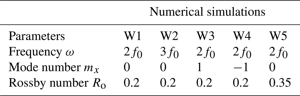
Five numerical simulations of the RSW equations, i.e. Eq. (1), featuring a plane wave interacting with a zonal jet have been performed. The parameters that vary from one simulation to another are the temporal frequency of the incoming wave, its direction of propagation, and the Rossby number of the turbulent jet – see Table 1. The simulations are labelled W1, which is the reference simulation, and W2 to W5. The Burger number is B_u=1 for all simulations (the unit for space coordinates is therefore the Rossby radius of deformation), and β=0.05. The wave amplitude is small, such that wave–wave interactions are negligible. For W1–W4, the jet has approximately the same spectrum and the same energy level, and only the impact of different wave parameters is studied for these runs.

Table 1 Parameters of the different simulations.

The equations have been discretised using a spectral method in space and a Runge–Kutta time scheme with the open-source code Dedalus (Burns et al., 2020). The domain Ω is a rectangular domain of size $[\mathrm{0},\mathrm{20}]\times [-\mathrm{20},\mathrm{20}]$, discretised on a 128 × 256 grid for W1–W4 and on a 256 × 1024 grid for W5, which requires a higher resolution. To simulate open boundaries, “sponge layers” are considered, in which the various fields are damped at both edges of the domain in the y direction (grey area in Fig 2). These regions are a numerical artifice that delimit the “physical” domain where $\left|y\right|<\mathrm{12}$. In particular, βy is linear in the physical domain, and periodicity of the Coriolis term is ensured in the sponge region through a smooth recovery function, thus allowing the use of a Fourier basis in a non-homogeneous direction. As these regions are not physical, they are not included in the different POD calculations.

All simulations are initialised with an eastward zonal jet at geostrophic equilibrium with a small perturbation superimposed to trigger its destabilisation. An eastward-wind forcing term, which is constant in time and follows a Gaussian function in y, and a radiative-damping term of the form αh (where $\mathit{\alpha }={\mathrm{10}}^{-\mathrm{3}}$) are added to the system in order to maintain the balanced current in a statistically stationary state (e.g. Brunet and Vautard, 1996). To ensure numerical stability, a small hyperviscosity diffusion term $-R_{\mathrm{o}}/R_{\mathrm{e}}\frac{\mathrm{1}}{\mathrm{1}+R_{\mathrm{o}}h}{\mathrm{\nabla }}^{\mathrm{4}}$ is also added in the momentum equations, with $R_{\mathrm{e}}=\mathrm{2}\cdot {\mathrm{10}}^{\mathrm{5}}$, following (Ochoa et al., 2011). Furthermore, the wave field is generated (and re-absorbed in the north) in the sponge layers by nudging toward the incoming plane wave solution – see the visualisation given in Fig. 2.

The model is first run without wave forcing. Once stationarity is reached (after $\mathrm{4000}{f}_{\mathrm{0}}^{-\mathrm{1}}$, which corresponds approximately to 450 d at mid-latitudes), we activate the generation of a plane wave in the sponge layers at the bottom of the domain, which propagates along y before interacting with the jet. The properties of the wave forcing follow the dispersion and polarisation relations computed from the harmonic solutions of Eq. (1) linearised around a state at rest. This second phase of simulation is $\mathrm{4000}{f}_{\mathrm{0}}^{-\mathrm{1}}$ long for W1–W4 and $\mathrm{8000}{f}_{\mathrm{0}}^{-\mathrm{1}}$ long for W5. Snapshots are saved every $\mathrm{1}/\mathrm{10}$th of a wave period, enabling extraction of the wave field. The mesoscale part is then extracted (offline) using a low-pass filter (fourth-order Butterworth) with a cutoff frequency of $\mathrm{2}\mathit{\pi }/\mathrm{10}{f}_{\mathrm{0}}^{-\mathrm{1}}$ (approximately corresponding to a period of 3 d at mid-latitudes), and the wave field is extracted by complex demodulation at frequency ω (and using the same low-pass filter).

Figure 1 shows the power spectrum of the SSH field, computed using the Welch method, with a Hann window of size 160 $f_{\mathrm{0}}^{-\mathrm{1}}$ (512 snapshots) and with 50 % overlap. It clearly exhibits two broadband spectral peaks: one around ω=0, associated with the jet, and another around ω=2, associated with the wave. This highlights the timescale separation between both flow components that we discussed in Sect. 2. We point out that sub-mesoscale contributions are also extracted by means of complex demodulation, but these remain negligible. One may also notice that the SSH contribution of the wave is only 1 %–2 % of that of the low-frequency turbulent flow, as well as of the presence of a weak super-harmonic signal (at ω=4f₀), which we do not consider in this study.

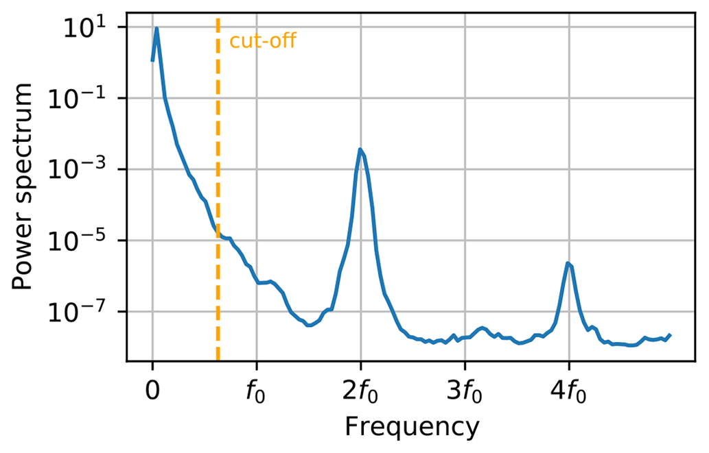
Figure 1 Power spectrum of the SSH field in lin–log scale, in the centre of the domain at x=10 and y=0, for W1. The dotted orange line indicates the filter cut-off frequency.

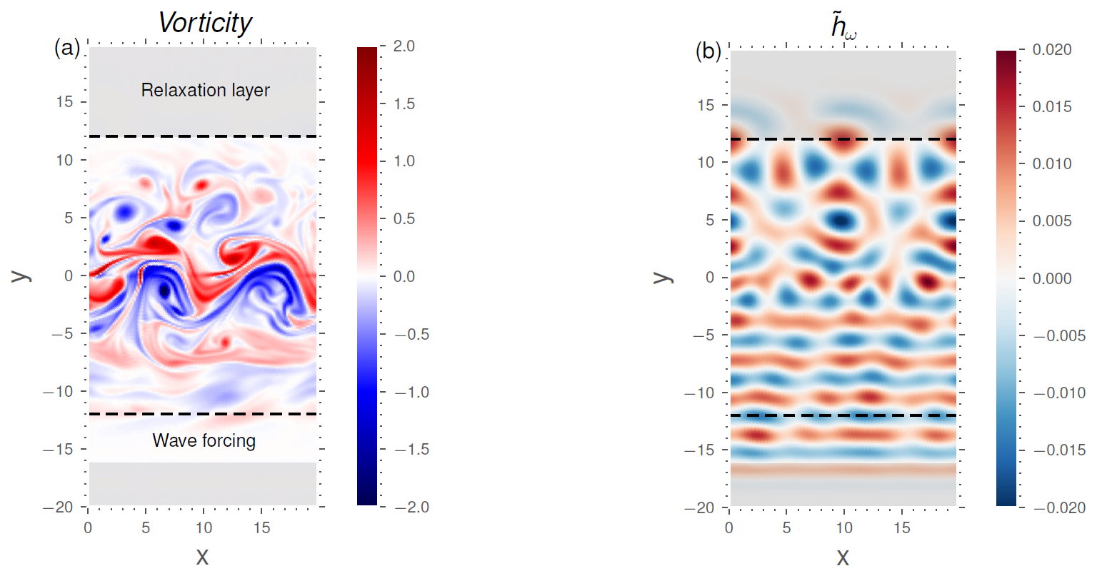
Figure 2 Snapshots of the reference simulation W1 with ω=2f₀, m_x=0: (a) total vorticity field and (b) complex amplitude of the wave SSH contribution. The sponge layer is included in this visualisation for $\left|y\right|>\mathrm{12}$, with the wave forcing region to the south and the relaxation layer to the north and south.

A snapshot of the vorticity field and the complex amplitude of the SSH of the northward-propagating wave for the reference simulation is displayed in Fig. 2. It shows that the incident wave to the south of the domain is almost a plane wave, while more disorganised patterns are visible in the north of the domain, which is the signature of the loss of coherence caused by the interaction with the mesoscale flow.

4.2 BBPOD and EPOD analysis

In this section, we show and discuss how the BBPOD and EPOD methods perform in extracting the variability of the wave field, and we provide some information on the underlying mechanisms. The modes are computed in the physical domain, discarding the sponge regions (for $\left|y\right|>\mathrm{12}$).

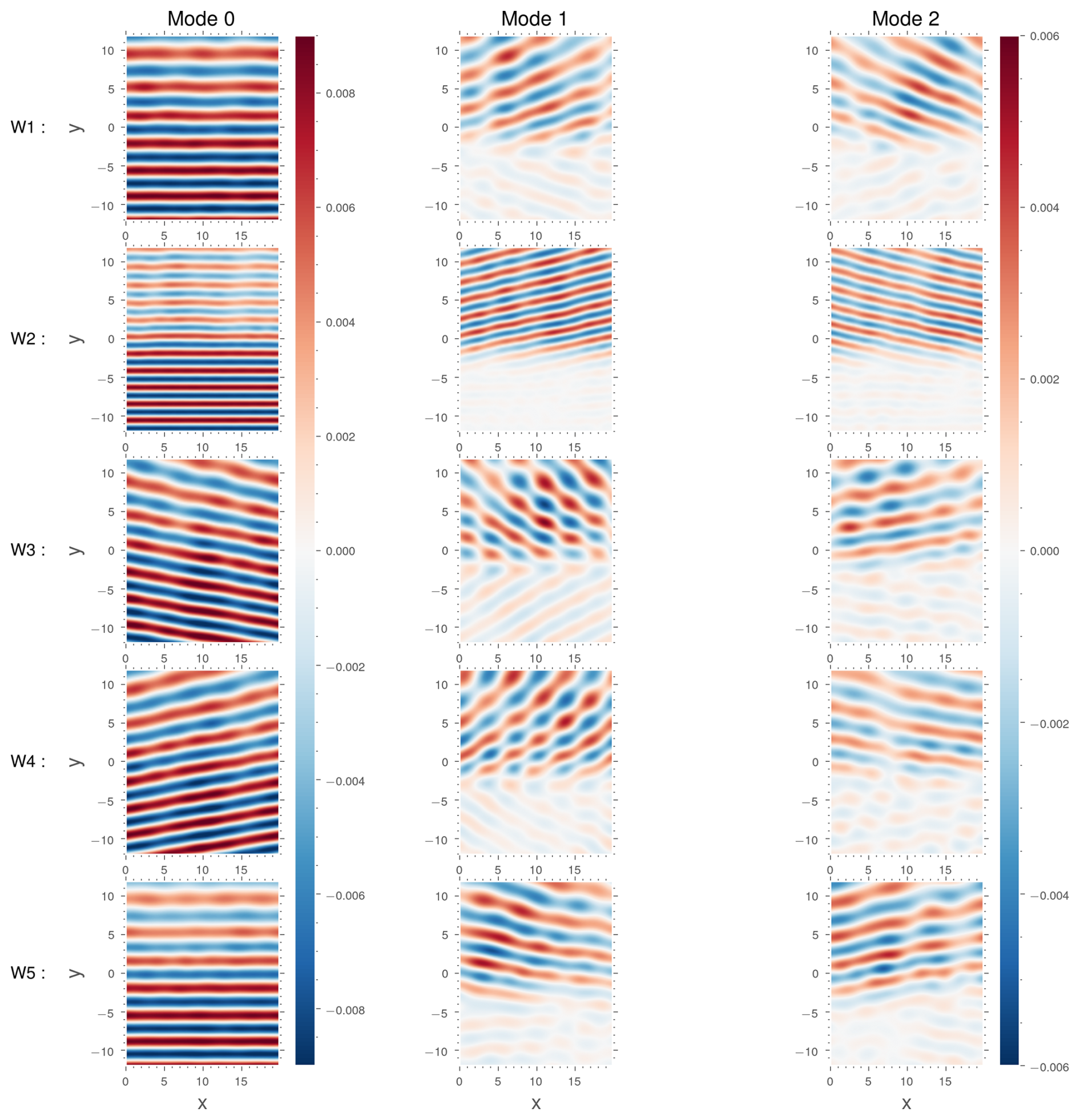
Figure 3 The three dominant weighted BBPOD modes of SSH (left to right), calculated as $\sqrt{{\mathit{\lambda }}_{n,\mathit{\omega }}}{\mathit{\psi }}_{n,\mathit{\omega }}$ for the runs W1 to W5 (top to bottom).

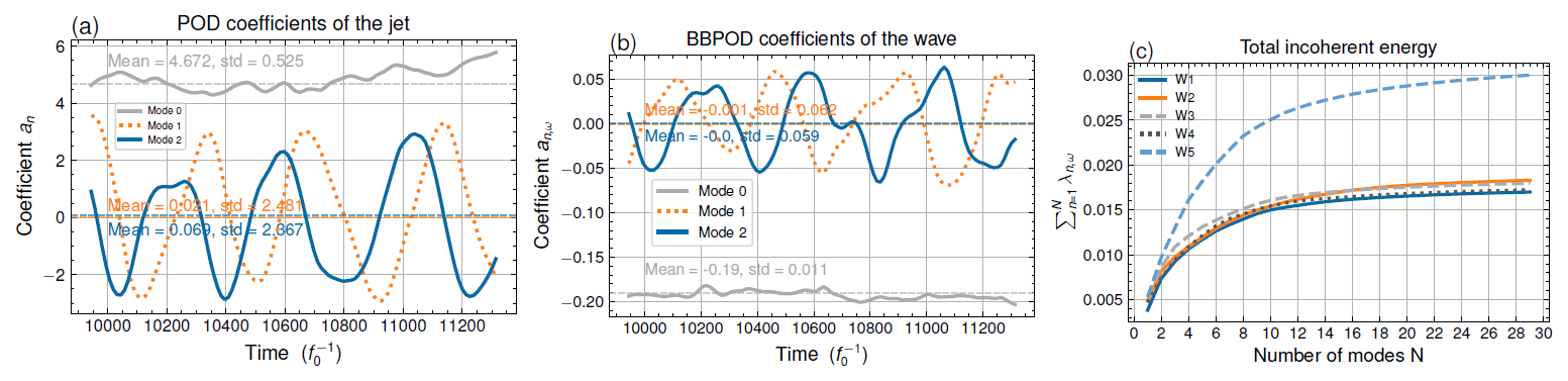
Figure 4 (a) The three leading POD coefficient of the jet: $a_n=({\mathit{q}}_{\text{jet}},{\mathit{\psi }}_n{)}_{W_E}$. (b) The three leading BBPOD coefficient of the wave $a_{n,\mathit{\omega }}=({\stackrel{\mathrm{̃}}{\mathit{q}}}_{\mathit{\omega }},{\mathit{\psi }}_{n,\mathit{\omega }}{)}_{{\mathbf{W}}_E}$. These are computed based on the reference run W1, and the respective mean values and root-mean-squared errors are shown. (c) Modal cumulative incoherent energy ${\sum }_{n=\mathrm{1}}^N{\mathit{\lambda }}_{n,\mathit{\omega }}$ of the different runs.

4.2.1 BBPOD analysis of the wave field

Figure 3 shows the SSH component of the first three weighted BBPOD modes $\left(\sqrt{{\mathit{\lambda }}_{n,\mathit{\omega }}}{\mathit{\psi }}_{n,\mathit{\omega }}\right)$ of the wave field for every simulation. The first dominant mode (the most energetic), in the first column, corresponds to harmonic waves propagating in the same direction as the incident wave. It corresponds to the coherent part of the wave, as confirmed by the time series of the corresponding projection, which is nearly constant in time (see Fig. 4b). We should mention that the fact that the coherent wave is captured by the first BBPOD mode is not guaranteed a priori. Here, it occurs because the energy is integrated over the whole domain, including the lower half of the domain where wave propagation is essentially coherent. We can also note a slight damping of the amplitude of the coherent mode for the W2 and W5 simulations, where the wave is subject to greater interactions. This damping can be interpreted as resulting from the wave–mesoscale correction (last right-hand-side term in Eq. 11a).

The sub-optimal modes represent contributions from the incoherent wave; i.e. they are a residue of the coherent part, which is decorrelated from the wave forcing. The first two dominant incoherent modes exhibit nearly plane waves deflected by the jet in the upper part of the domain in several directions (where we can also note weak reflections by the jet in the lower half of the domain).

These x-wise structures of these waves are very close to Fourier modes associated with a pair of wavenumbers $m_x=k_x{L}_x/\mathrm{2}\mathit{\pi }$ that are, from top to bottom, $(-\mathrm{2},\mathrm{2}),(-\mathrm{2},\mathrm{2}),(\mathrm{3},-\mathrm{1}),(-\mathrm{3},\mathrm{1})$. This is a consequence of the statistical homogeneity of our configuration (periodic domain, zonal jet); i.e. the statistics do not depend on x. This statistical property ensures that the BBPOD modes converge to Fourier modes in x as the number of snapshots of the correlation matrix increases (Schmidt and Colonius, 2020).

Calculating the eigenvalues of the correlation matrix gives the average energy contribution of each mode (Eq. 18). We show (in Fig. 4c) the cumulative energy of the incoherent part as a function of the number of modes. This corresponds to the energy contained in the first N incoherent and/or sub-optimal modes, equal to ${\sum }_{n=\mathrm{1}}^N{\mathit{\lambda }}_{n,\mathit{\omega }}$, whereas λ_0,ω refers to the energy of the coherent mode. The figure shows, first of all, that the W5 simulation represents a more energetic incoherent wave than in the other simulations. This can be explained by the fact that the Rossby number is higher, and, therefore, the contribution of the non-linear terms between the wave and the jet responsible for the loss of coherence is, a priori, also higher (Eq. 13). Secondly, the figure shows that the incoherent waves from the W1–W4 simulations have a comparable energy level as the jet is approximately the same.

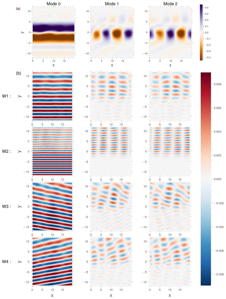
Figure 5 Three leading POD modes of the jet (a) and the associated EPOD modes of the wave field (b) for simulations W1–W4. They are weighted by the square root of the respective POD eigenvalue of the jet $\sqrt{{\mathit{\lambda }}_n}$. The first three eigenvalues are λ₀=22.13, λ₁=6.09, λ₂=5.59 for W1 and λ₀=22.65, λ₁=6.77, λ₂=6.55 for W2.

4.2.2 EPOD analysis

Figure 5 shows the first three dominant jet POD modes and the associated wave EPOD modes for simulations W1 to W4. Akin to the dominant wave BBPOD mode shown previously, the first POD mode of the jet is approximately the mean field and has nearly constant projection coefficients (Fig. 4b). The two sub-optimal modes are meanders in phase quadrature. The first EPOD mode of the wave, which is correlated with the mean field, corresponds to the coherent part and has a spatial structure that is very similar to that of the first BBPOD mode. The second and third EPOD modes represent the parts correlated with the meanders of the jet and feature standing-wave patterns along x, which are also in phase quadrature, suggesting a slow zonal propagation velocity following the jet. This is pronounced in simulations where the wave crosses the jet perpendicularly (W1, W2), with four nodes in the domain. For the W5 high-Rossby-number simulation (shown in Appendix C), the jet's sub-optimal modes also represent meanders, and the wave EPOD modes are standing-wave patterns, both with doubled wavelengths compared to runs W1–W4.

The correspondence between the wavelengths of the jet meanders and those of the EPOD modes confirms the analytical link between these structures that we discussed in Sect. 3.2 (see Eq. 21). The dominant wave EPOD modes appear to be the response to interactions between the coherent part and the jet POD modes. The validity of this equivalence suggests that the multiple-interaction term is weak for all simulations, which reflects the fact that the mesoscale fluctuations are confined y-wise, such that the scattered wave rapidly leaves this zone, leaving no room for further interaction with the fluctuating jet.

The temporal evolution of the BBPOD wave modes seems to be related to the EPOD–POD behaviour – see Fig. 4: the first modes are approximately in phase, and the second modes are approximately in phase opposition. Indeed, the standing waves of EPOD modes correspond to the superposition of the upward and downward deflections extracted by the BBPOD method. More precisely, BBPOD extracts these two deviations separately since they are decorrelated and associated with opposite-sign wave numbers, whereas the EPOD method extracts the superposition of these deviations in a single mode by correlation with the jet. It can be noticed in Fig. 4b that there is a slight phase shift from an exact phase opposition, which corresponds to the slow zonal propagation of the standing wave. By summing these two first modes, we can conclude that the contribution of these meandering modes to the incoherent wave represents between 40 %–50 % of the incoherent energy for W1–W4 and 30 % for W5 (Fig. 4c).

In conclusion, we have shown that the proposed statistical methods – BBPOD and EPOD – allow us to extract and interpret a wave field scattered by mesoscale turbulence. In particular, they allows us to quantify the energetic contribution of the dominant modes of variability of the wave field in connection with the variability of the mesoscale flow. The EPOD shows that the meanders of the mesoscale jet generate an incoherent wave in the form of a standing wave, made up of deviations in directions determined by the primary interactions.

4.3 Estimation

The second part of this study is dedicated to the problem of estimation, implementing the algorithm (Algorithm 1) introduced in the previous section. Most of the results are shown for the W1 reference simulation. The time series are divided into a learning window and a test window, the durations of which (for the W1 run) are ≈ 1300 wave periods (16 months) and ≈ 200 wave periods (50 snapshots separated by four wave periods), respectively. For the sake of simplicity, the estimate of the wave is based on the estimate of its complex amplitude as the total wave can be reconstructed without losing accuracy (using Eq. 2).

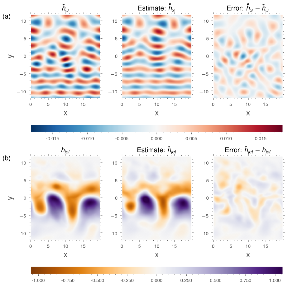
Figure 6 Estimate of the SSH contribution of the wave (a) and of the jet (b) for 30 modes from one snapshot for W1.

4.3.1 Estimation from a full SSH observation

Figure 6 shows an estimate of the SSH component of the wave and mesoscale fields, calculated from a complete SSH observation using 30 POD–EPOD modes. Qualitatively, the estimation is in good agrement with the reference, and the error does not exhibit any particular structure or bias.

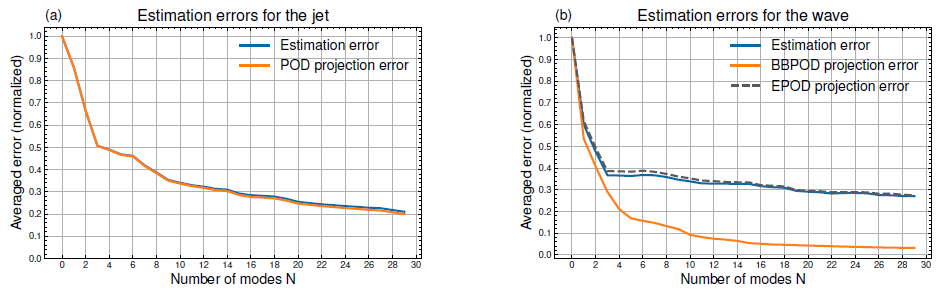
Figure 7 Time-averaged L² norm errors (blue) as a function of mode numbers included, together with the projection error of the corresponding POD decompositions, for the turbulent jet (a) and the wave field (b). For the wave, the EPOD decomposition Eq. (20) is also plotted (dotted line). The results correspond to the W1 run.

The accuracy of the estimate (with respect to the number of modes considered) is quantified via the L² norm of the error, averaged over the entire test window, for the complex wave amplitude, $\langle \Vert {\widehat{\stackrel{\mathrm{̃}}{\mathit{q}}}}_{\mathit{\omega }}-{\stackrel{\mathrm{̃}}{\mathit{q}}}_{\mathit{\omega }}{\Vert }_{L^{\mathrm{2}}}^{\mathrm{2}}\rangle /\langle \Vert {\stackrel{\mathrm{̃}}{\mathit{q}}}_{\mathit{\omega }}{\Vert }_{L^{\mathrm{2}}}^{\mathrm{2}}\rangle$, and for the mesoscale part, $\langle \Vert {\widehat{\mathit{q}}}_{\text{jet}}-{\mathit{q}}_{\text{jet}}{\Vert }_{L^{\mathrm{2}}}^{\mathrm{2}}\rangle /\langle \Vert {\mathit{q}}_{\text{jet}}{\Vert }_{L^{\mathrm{2}}}^{\mathrm{2}}\rangle$ (Fig. 7). The estimation error is compared with the averaged projection error performed when the jet is projected onto its POD basis and when the wave is projected onto its BBPOD basis. Indeed, the projection error measures the ability of the basis learnt from the training window to span the observations from the test window: it indicates the maximum energy that can be captured by N modes (this is an inherent property of the POD) and thereby provides a minimal bound for the estimation error. Also shown is the EPOD projection error, which corresponds to the error between the true complex amplitude field and a decomposition over N extended modes, wherein the coefficients are calculated by means of projection of the jet onto its POD basis.

We see in Fig. 7 that the estimation error decreases over the first 30 modes for each of the fields. Using 30 modes, 80 % of the mesoscale energy is captured. For the wave (Fig. 7a), the estimate captures around 73 % of the total energy and 63 % of the incoherent energy (associated with the norm defined in Eq. 15). The total coherent energy of the test window corresponds to the energy captured by the projection of the wave field onto the first BBPOD mode, which is 46 %. The total incoherent energy corresponds to the residual, and the incoherent estimate corresponds to the estimate of the sub-optimal EPOD modes. The error reduction decreases as the number of modes increases, which is very fast until N=5, and then continues to decrease progressively. This indicates a cost–accuracy trade-off, which is usual in model reduction and which leaves room for tuning as a function of targeted model performances. Furthermore, we observe that the two error estimates (for the mesoscale and the wave) have a similar shape, with a clear break in slope from the third mode, with modes 2 and 3 corresponding to the meandering of the jet and the associated response in the form of a standing wave for the wave (see Sect. 4.2), which reflects the fact that the dynamics of both motions are coupled.

For the mesoscale (Fig. 7a), since the POD basis is optimal and the SSH field is mainly dominated by the turbulent jet, the estimation and projection errors collapse. This suggests that the jet coefficients – including for the velocity component, included in the error norm – are perfectly estimated. This shows that the SSH is sufficient to estimate the jet flow, which is consistent with the fact that the jet is almost in geostrophic balance. For the wave estimate (Fig. 7b), one sees a difference between the estimation error and the BBPOD projection error. Already for the first mode (corresponding to the coherent part), there is approximately 8 % of the total energy missing in the estimate. There are several possible explanations for this: firstly, the wave estimate only contains the part that is correlated with the jet and not the part that is decorrelated. Also missing is the fraction of the wave field correlated with the residual of the jet estimate over the 30 POD modes (representing 20 % of the jet's energy). Secondly, non-stationarity effects in the flow can partially degrade the estimation of correlations between the wave and the jet. Despite the limitations that have been mentioned, we see that, for a total observation of SSH, one can have confidence in a large number of modes with regard to estimating the wave and jet fields.

Table 2 Highest average energy captured over the first 30 modes for wave and jet estimation for simulations W1–W5. For W1, this value can also be seen in Fig. 7, which is reached with a consideration of the first 30 modes.

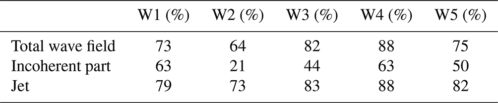
The wave estimation error presented above is calculated for each simulation, W1–W5, in Table 2. The numbers shown correspond to the minimum of the error as a function of the number of modes for the first 30 modes (corresponding to the maximum energy captured). With the exception of the W2 simulation, which represents a wave of higher frequency compared to the other runs, the method captures more than 73 % of the total wave energy for each of the simulations and between 44 % and 63 % of the incoherent energy. Moreover, the wave estimate does not diverge as the number of modes increases for these simulations. However, the method seems less effective at capturing a higher-frequency wave by means of correlation in the W2 simulation. The best estimate is reached in the 12th mode and diverges very slightly. Unfortunately, we do not have a clear explanation for this. We can simply point out that, at high frequencies (with ω=3f₀ being greater than M₄≈2.8f₀ at mid-latitudes), the scattering of waves is more complex and more intense (Ward and Dewar, 2010). The estimate of the jet remains fairly robust since its amplitude remains high for all the simulations. We can also confirm that, by construction of the method, the better the estimate of the jet, the better the estimate of the total wave.

4.3.2 Impact of a partial observation

In the final part of the study, we evaluate the sensitivity of the method to the spatial coverage of observations. Figure 8 shows an example of a subsampled observation, consisting of four SSH vertical bands that are approximately homogeneously spaced in the domain and one Rossby radius in width.

Figure 8 Sparse SSH snapshot observation from the W1 run, covering 20 % of the full domain.

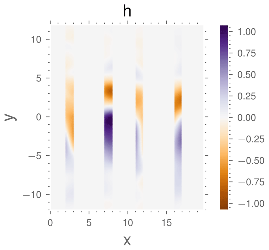
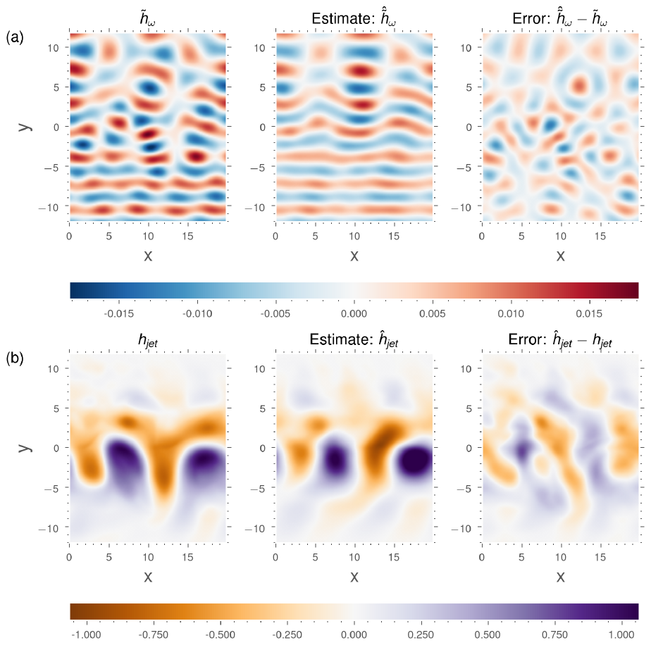
Figure 9 Estimate of the SSH contribution of the wave (a) and of the jet (b) for 12 modes from one sparse snapshot.

Figure 9 shows an estimate over 12 EPOD and POD modes from the same snapshot as in the full-observation case of the complex amplitude of the wave and the jet. Since fewer modes have been taken into account for the estimation, the wave field is smoother, but the error is still qualitatively quite small. For the jet, the error is more pronounced, with higher amplitudes than in the case of total observation. The choice of 12 modes corresponds approximately to the minimum error, as shown below.

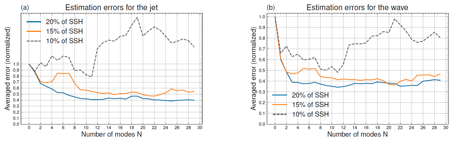
Figure 10 Time-averaged L² norm errors for the jet (a) and the wave (b) for sparse observations. Three types of spatial domain coverages are considered (10 %–15 %–20 %).

We calculate (see Fig. 10) the jet and wave estimation errors in the L² norm averaged temporally over the whole test window. We evaluate the sensitivity of the error by varying the observation coverage from four bands (covering 20 % of the domain) to two bands (10 % of the domain). With four vertical bands, the algorithm is still able to estimate the first three modes with little difference compared to the total observation. These modes correspond to larger jet structures and therefore seem to be less affected by the degradation of the spatial sampling. From three modes, the estimate reaches a plateau for the wave and decreases slightly for the jet. At best, around 60 % of the jet's energy is captured, and around 65 % of the wave's energy is captured. For three vertical bands, the error deteriorates slightly, but the curves remain similar to the previous case. Finally, the case of two bands is more pathological and shows that, when the observation space is too small and the number of parameters to be minimised is too large (here > 11 modes), the error increases. In addition, as in the case of total observations, we note that the coupling of the projection coefficients between the jet and the wave means that the error curves for the jet and the wave necessarily follow a similar trajectory, suggesting that a good estimate of the jet is required in order to have a good estimate of the wave. The increase in the error could be mitigated by adding regularising terms to the algorithm, e.g. penalising the amplitude of high modes.

4.4 Discussion

The EPOD-based estimation method presented above relies on the correlation between the mesoscale fluctuations and the scattered-wave field to estimate the latter in a regime where the SSH is dominated by the mesoscale, which is probably the main advantage of the method. To emphasise this, an attempt is made to estimate and separate the mesoscale and wave dynamics from single SSH snapshots using a simpler approach, which is detailed in Appendix B. This involves considering BBPOD modes (with a specific set of projection coefficients to be determined by optimisation) instead of EPOD modes to express the wave. This approach fails completely in reconstructing the wave field (Fig. B1 in the Appendix). Although making these two bases independent could provide a better projection space (which, here, is optimal in terms of energy content), the estimation fails because (i) it subjects the minimisation problem to overfitting; (ii) it discards the statistical links between the two bases supported by their dynamical relation, as seen in Eq. (21); and (iii) the wave is poorly observed due to a large relative amplitude difference between the SSH contribution of the jet and the wave. Thus, this comparison highlights the benefit of explicitly accounting for the coupling between the mesoscale and the wave via extended modes.

Let us now discuss the limitations of the proposed approach. First, the EPOD decomposition of the wave only provides an estimate of the part of the wave that correlates with a truncated POD decomposition of the jet. As discussed above, this contribution is a priori important for an incoherent wave resulting from interaction with a turbulent flow and if the number of modes included in the decomposition is sufficiently large. Secondly, the decomposition bases should be able to span future observations that have not been learnt from the dataset. Some of the errors may, therefore, be due to errors in projecting the wave and jet observations onto their respective bases.

Finally, it can be expected that this approach would become inefficient in configurations where the signature of the IT becomes dominant and, in particular, in regimes with very weak mesoscale flows as the correlation between the mesoscale fluctuations and the wave field would be less pronounced. In this case, recourse to a BBPOD-based algorithm seems more appropriate, provided some improvements are achieved, such as the use of regularisation techniques in the minimisation algorithm to avoid overfitting. For example, Egbert and Erofeeva (2021) showed that a SPOD basis can be used to estimate part of the incoherent signal off the Amazon using multiple snapshots. Their algorithm estimates the sea surface height (SSH) contribution of the internal tide by finding the IT projection coefficients that minimise the error with multiple observations.

Constructing an algorithm that takes advantage of each method depending on the dynamical regime is a straightforward development that is left for future work. In any case, more sophisticated minimisation algorithms that better constrain the temporal coefficients need to be implemented in order to maintain accuracy as observations degrade. This may include a regularisation term, e.g. that penalises higher mode amplitudes, depending on the choice of an appropriate norm and an initial guess regarding the solution. In a sense, the methods proposed by Egbert and Erofeeva (2021) or Tchilibou et al. (2024) are examples of constraints put on the temporal coefficient by using a harmonic function to link observations at different times.

5 Conclusions and perspectives

In this study, we have proposed new data-driven statistical decompositions of a (internal) wave scattered by mesoscale turbulence. These decompositions are derived from the POD and describe the slow evolution of the complex amplitude of the wave, driven by non-linear interactions with the mesoscale flow. We first introduced the broadband POD, which adapts the POD for a scattered-wave field with a broadband spectrum. Then, we proposed a decomposition of the wave field that extracts its fraction correlated with the jet using the extended POD (EPOD) method, which is probably the most important aspect of this study. We have highlighted a dynamic link that exists between the extended wave modes and the mesoscale POD modes, which holds under certain wave-scattering regimes (dominant and localised primary interactions) and allows for a physical interpretation of the extended modes.

We have demonstrated, using idealised rotating-shallow-water simulations, the ability of both decompositions to analyse the scattering of a low-amplitude wave by a zonal jet. For different wave and mesoscale fields, the dominant BBPOD modes of the wave result from the interactions between the dominant mesoscale POD modes and the coherent part of the wave. A significant part of the incoherent wave is a standing wave generated by the meanders of the jet, determined by these primary interactions.

In the second part of this study, we addressed the issue of the disentanglement of waves and mesoscale flows from a single SSH snapshot. Our method relies on a simple minimisation algorithm, wherein the SSH observation is expressed as the sum of a mesoscale contribution, decomposed on a POD basis, and a wave contribution correlated with the jet, decomposed based on the extended POD mode. This coupled POD–EPOD estimation algorithm allows us to estimate a total wave field, with its velocities, which is of very low amplitude (especially compared to the mesoscale contribution) from isolated SSH snapshots. This allows us to estimate the incoherent-wave field (we captured between 44 % and 63 % of the incoherent-wave energy in the idealised RSW simulations), which can potentially give us access to derived quantities such as incoherent-wave energy fluxes.

Although this study was primarily motivated by the issue of estimating internal tides, the EPOD method has a fairly general formalism that could be applied to different types of waves scattered by a time-varying flow, provided we can extract from data the variable envelope of the scattered wave. This includes, for example, the scattering of near-inertial waves propagating in the ocean, as studied in Danioux and Vanneste (2016); Young and Jelloul (1997), with the propagation of the slowly varying wave envelope being modelled here, along with the loss of coherence in the barotropic tide in coastal areas or the scattering of acoustic waves by turbulence (Thomas, 2017). Also, this method could be applied to waves of large amplitude since they remain correlated with the turbulent flow, which is a straightforward extension of this study.

Finally, an extension of this method to the study of a scattered wave in three dimensions, e.g. as in Kafiabad et al. (2019), may be envisaged. Although EPOD modes can be defined in 3D, it seems appropriate to apply our method to a set of 2D RSW models similar to the ones in this study after projecting a 3D model onto a vertical-mode basis, which is widely used and relevant for the study of ITs (Dunphy et al., 2017; Kelly et al., 2016).

Another important part of this study is the adaptation of these methods to more realistic cases. A few limitations need to be addressed in order to achieve this. First, the use of instantaneous correlation between the jet and the wave is mainly valid for estimating the wave locally. It is also necessary to develop techniques to improve the convergence of statistical estimates, which is not achieved when the number of snapshots in the training time series is limited. One consequence of this convergence problem is that the proposed decompositions do not generate a space of sufficiently large dimension to estimate wave and jet observations. In particular, these techniques would improve the estimation of observations whose variability has not been sufficiently learnt from the reduced-size time series and that are not represented in the set of POD–EPOD modes. These techniques would also make it possible to extend the estimation of waves and currents to the scale of an ocean. Localisation techniques, which broadly consist of defining localised sub-domains to enable the consideration of localised interactions and an artificial increase in the number of samples, could address these issues (Hamill et al., 2001; Farchi and Bocquet, 2019). Another methodological challenge with regard to addressing more realistic configurations is the fact that the internal-tide field contains several nearby frequencies. How to separate each coherent peak in the data and adequately describe their correlation with the turbulent flow remains to be understood. Therefore, we think that further work on idealised cases is required before applying this method to a realistic case.

Appendix A: Equivalence between broadband POD and SPOD

This Appendix presents the algorithmic specificities of the common SPOD algorithm using the Welch method (Welch, 1967) to estimate the cross-spectral density matrix (CSD) and its relation to the BBPOD algorithm that is used in this study. For some well-chosen parameters, we show that the two algorithms are equivalent.

The following proof is performed with discrete variables, considering a signal x_t with time spacing Δt and t_k=kΔt.

.

The complex demodulation is written as

$$\begin{array}{}\text{(A1)}& \begin{array}{rl}{\stackrel{\mathrm{‾}}{x_t{e}^{-i\mathit{\omega }t}}}_j& =\sum _{k=-m}^m{b}_k{x}_{j-k}{e}^{-i\mathit{\omega }tj-k}\\ & =\sum _{k=j-m}^{j+m}{b}_{j-k}{x}_k{e}^{-i\mathit{\omega }{t}_k},\end{array}\end{array}$$

where $(b_i{)}_{-m\le i\le m}$ denotes the discrete coefficients of the filter $\stackrel{\mathrm{‾}}{\cdot }$.

Besides this, the principle of the Welch method is to subdivide x_t into possibly overlapping blocks of size N, with an overlap N_o. A fast Fourier transform (FFT) is then performed on each windowed block to extract the Fourier component at the tidal frequency, denoted as $X_{\mathit{\omega }}^l$, where l is the block index. So,

$$\begin{array}{}\text{(A2)}& X_{\mathit{\omega }}^l=\sum _{k=-N/\mathrm{2}}^{N/\mathrm{2}}{x}_{k+l(N-N_{\mathrm{o}})}{W}_k{e}^{-i\mathit{\omega }{t}_k},\end{array}$$

where W_k is a window function defined based on $[-N/\mathrm{2},N/\mathrm{2}]$.

By changing the variable $k^{\prime }=k+l(N-N_{\mathrm{o}})$, it follows that

$$\begin{array}{}\text{(A3)}& X_{\mathit{\omega }}^l=e^{i\mathit{\omega }{t}_{l(N-N_{\mathrm{o}})}}\sum _{k^{\prime }=l(N-N_{\mathrm{o}})-N/\mathrm{2}}^{l(N-N_{\mathrm{o}})+N/\mathrm{2}}{x}_{k^{\prime }}{W}_{k^{\prime }-l(N-N_{\mathrm{o}})}{e}^{-i\mathit{\omega }{t}_{k^{\prime }}}.\end{array}$$

Assuming that the window function is symmetric in the middle of each block (which is verified for most windows used in the literature), i.e. $W_k=W_{-k}$, Eq. (A3) gives

$$\begin{array}{}\text{(A4)}& X_{\mathit{\omega }}^l=e^{i\mathit{\omega }{t}_{l(N-N_{\mathrm{o}})}}\sum _{k^{\prime }=l(N-N_{\mathrm{o}})-N/\mathrm{2}}^{l(N-N_{\mathrm{o}})+N/\mathrm{2}}{W}_{l(N-N_{\mathrm{o}})-k^{\prime }}{x}_{k^{\prime }}{e}^{-i\mathit{\omega }{t}_{k^{\prime }}}.\end{array}$$

Finally, by choosing the window function as the filter coefficients, i.e. W_k=b_k and $m=\frac{N}{\mathrm{2}}$, in relation to Eq. (A1) yields

$$\begin{array}{}\text{(A5)}& X_{\mathit{\omega }}^l=e^{i\mathit{\omega }{t}_{l(N-N_{\mathrm{o}})}}{\stackrel{\mathrm{‾}}{x_t{e}^{-i\mathit{\omega }t}}}_{l(N-N_{\mathrm{o}})}.\end{array}$$

Consequently, up to a phase, the FFT of a block l of size N with overlap N_o at ω corresponds to the complex demodulation of the signal at time l(N−N_o). The phase shift is cancelled when computing the correlation over N_b blocks:

$$\begin{array}{}\text{(A6)}& \sum _{l=\mathrm{0}}^{N_{\mathrm{b}}}{X}_{\mathit{\omega }}^l{X_{\mathit{\omega }}^l}^{\ast }=\sum _{l=\mathrm{0}}^{N_{\mathrm{b}}}{\stackrel{\mathrm{‾}}{x_t{e}^{-i\mathit{\omega }t}}}_{l(N-N_{\mathrm{o}})}{\stackrel{\mathrm{‾}}{x_t{e}^{-i\mathit{\omega }t}}}_{l(N-N_{\mathrm{o}})}^{\ast }.\end{array}$$

Therefore, the Welch method computed with parameters $(N,N_{\mathrm{o}},N_{\mathrm{b}},W)$ is equivalent to computing the complex demodulation of the time series over N_b snapshots sampled every N−N₀ with a filter chosen as the common window function W (Hann, Hanning, etc.).

This simple proof highlights the fact that the window function in the Welch method is playing the role of the filter in the BBPOD method. Although the two methods are equivalent, they differ in terms of their use and interpretation and also in terms of the choice of parameters. BBPOD is designed to extract a broadband signal, the width of which is chosen via a filter using physical timescales. SPOD looks for an orthonormal basis for the Fourier coefficients at a given frequency, and the parameters of Welch's algorithm are chosen to minimise spectral leakage for a given amount of data. Techniques for reconstructing a broadband spectrum using several SPOD modes at each frequency of the spectrum are possible by reordering the energy contribution of modes at different frequencies (Nekkanti and Schmidt 2021). On the other hand, the orthogonality property of the modes is lost since the SPOD modes are no longer orthogonal at different frequencies.

Appendix B: Wave estimation using BBPOD instead of EPOD

A test has been performed in order to show the importance of informing the correlation between the jet contribution and the wave through EPOD in the estimation problem. Here, a “naive” algorithm is implemented, wherein the wave is decomposed on its optimal basis, BBPOD (instead of EPOD), while the jet is decomposed on its POD basis. Instead of considering the same coefficient a_n(t) for the jet POD mode and the wave EPOD mode, two independent sets of coefficients – a_n for the mesoscale and b_n for the wave – are sought through the optimisation algorithm, which is given by

$$\underset{(a_n,b_n)}{min}{\left|\sum _{n=\mathrm{0}}^{\mathrm{30}}{a}_n{\mathit{\psi }}_n({\mathit{q}}_{\text{jet}}{)}_h+\mathrm{\Re }\left[b_n({\mathit{\psi }}_{n,\mathit{\omega }}{)}_h{e}^{i\mathit{\omega }t}\right]-h\right|}^{\mathrm{2}}.$$

As is visible in Fig. B1, to be compared with Fig. 6, the corresponding estimate is completely wrong. Possible reasons for this failure are provided in the main text.

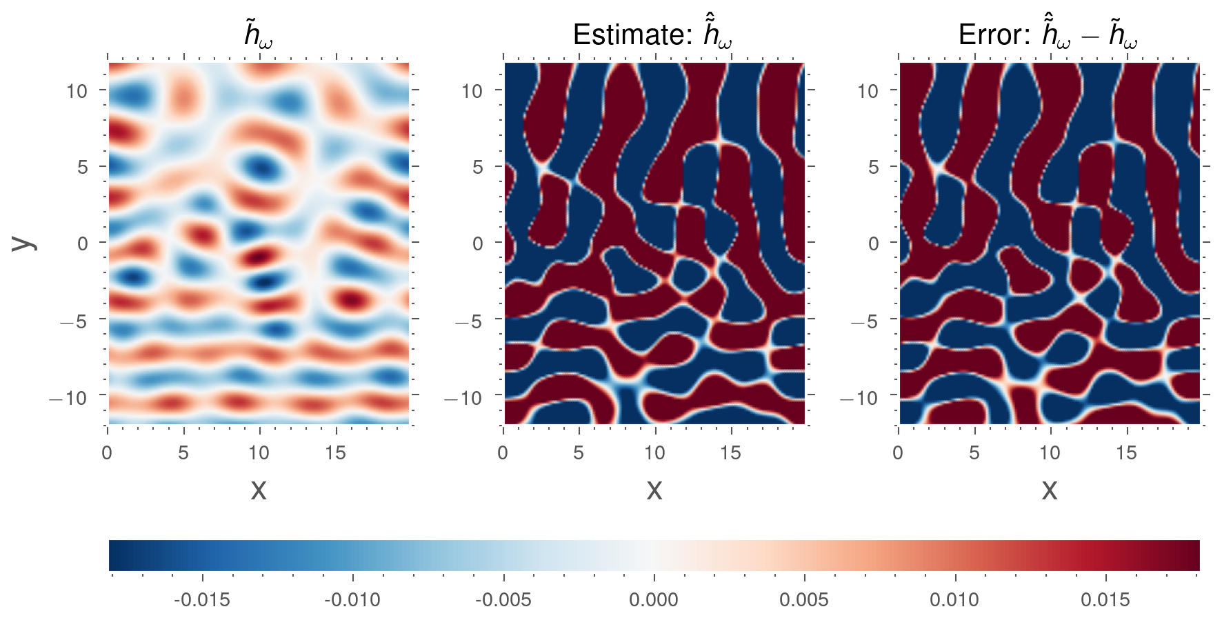
Figure B1 Estimation of the SSH contribution of the wave for the W1 run, computed from one snapshot, using 30 modes of the optimal basis of the jet and the wave vectors (POD for the jet and BBPOD for the wave).

Appendix C: Effect of Rossby number on the modal decompositions

In this section, we show the POD modes of the jet (Fig. C1a) and the EPOD modes of the wave (Fig. C1b) for the W5 simulation. This simulation is characterised by a higher Rossby number. The consequence is a change in the jet dynamics and then in the scattered-wave fields. This effect is visible in the results of the modal decompositions. The jet POD and wave EPOD modes show similar structures to W1–W4, but the wavelengths of modes 1 and 2 are twice as long.

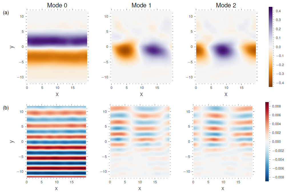
Figure C1 Three leading POD modes of the jet (a) and the associated EPOD modes of the wave field (b) for simulation W5. They are weighted by the square root of the respective POD eigenvalue $\sqrt{{\mathit{\lambda }}_n}$. The first three eigenvalues are ${\mathit{\lambda }}_{\mathrm{0}}=\mathrm{8.86},{\mathit{\lambda }}_{\mathrm{1}}=\mathrm{3.29},{\mathit{\lambda }}_{\mathrm{2}}=\mathrm{3.21}$.