Ocean wave spectrum bias correction through energy conservation for climate change impacts

A novel bias adjustment technique for 2D directional wave spectra is presented, which accounts for the intra-annual temporal variability of waves and the conservation of the wave energy integrated parameter and its extreme distribution, allowing for shifts in frequency and direction given by the global climate model and regional climate model (GCM–RCM) climate signal for the complete multimodal energy distribution. This work is the first attempt to address the biases inherent in GCM–RCM wave spectrum simulations for an assessment of the magnitudes of the projected changes in a climate change scenario. The bias-correction method is applied to a multimodel ensemble of 17 EURO-CORDEX regional simulations of wave spectra in 11 locations of the Mediterranean Sea. Climate change impacts are assessed by means of the changes between the bias-adjusted ensemble and hindcast wave spectra for mid-century conditions from 2034 until 2060 and end-of-century conditions from 2074 until 2100. The results highlight the need for novel bias-correction techniques that address the complexity of the possible directional and frequency shifts due to climate change, in order to provide an accurate assessment of projected future changes in the wave climate.

1 Introduction

Projected changes in wave climate due to shifts in atmospheric circulation have significant implications for coastal planning, adaptation, and mitigation strategies. Accurate representation of current and future wave climate, including its multimodal characteristics, is crucial for understanding coastal hazards and designing effective measures (IPCC, 2019; Oppenheimer et al., 2019). Several studies (Echevarria et al., 2019; Mortlock and Goodwin, 2015; Portilla-Yandún et al., 2016; Villas Bôas et al., 2017; Shimura and Mori, 2019) have highlighted the importance of resolving directional wave spectra when capturing the complexity of ocean waves and identifying different wave systems lacking in traditional studies of wave climate variability, which focus on integrated parameters such as significant wave height, mean wave period, and mean wave direction. Recently, Lobeto et al. (2021a) and Lira-Loarca and Besio (2022) presented studies on projections of 2D direction wave spectra in different locations around the world and in the Mediterranean Sea, respectively, and highlighted the importance of considering the multimodal behavior of waves for better understanding future changes in waves due to climate change.

Wave projections in climate change scenarios are usually generated by wave generation and propagation models driven by surface winds from global climate models (GCMs) or high-resolution dynamically downscaled surface winds from regional climate models (RCMs) (Morim et al., 2018; Jacob et al., 2020; Lira-Loarca et al., 2021b). However, systematic biases are present in GCM atmospheric simulations and RCM downscaling due to factors such as spatial resolution, simplified physics and parameterizations, internal variability, and downscaling processes (Christensen et al., 2008; Teutschbein and Seibert, 2012). Among the different outputs of GCMs and their regional downscaling GCM–RCMs, wind fields are known for depicting large uncertainties linked to their local-scale effect capture with only very high horizontal distributions, their spatial heterogeneity, and the challenge for climate models to accurately characterize the turbulent nature (Outten and Sobolowski, 2021). When using GCM–RCM wind field data to force wave climate projections, these biases and uncertainties are inherited, requiring the application of bias adjustment methods to ensure accurate coastal impact projections (Lemos et al., 2020b). Furthermore, the wave climate presents varying timescales ranging from decadal, intra-annual, to seasonal as well as storm events, swells, and wind waves exhibiting high temporal variability, which should be considered when applying bias correction techniques (Lira Loarca et al., 2023).

While bias correction techniques are widely used in studies involving climatic and hydrological variables such as precipitation and temperature (scalar variables varying in space and time), their application to the wave climate is found in a limited number of studies (Lemos et al., 2020b, a; Costoya et al., 2020; Lobeto et al., 2021b; Lira-Loarca et al., 2021a) and remains a challenging task due to the multivariate behavior and diverse temporal and spatial variability of waves. The wave climate is often defined by the main integrated wave parameters H_s (significant wave height), $T_{\mathrm{m}}/T_{\mathrm{p}}$ (mean or peak wave period), and ${\mathit{\theta }}_{\mathrm{m}}/{\mathit{\theta }}_{\mathrm{p}}$ (mean or peak wave direction), which are intrinsically correlated in both space and time and present, by themselves, a high temporal variability on different timescales. Lemos et al. (2020b) applied traditional bias adjustment techniques, such as the delta method, empirical quantile mapping (EQM), and empirical Gumbel quantile mapping (EGQM), to the univariate scalar variables, H_s, and they highlighted the performance of EGQM over the other methods in the characterization of extremely significant wave heights. Regarding the need to account for the temporal variability of the wave climate, Lira-Loarca et al. (2021a) compared the EQM method with the EQM-month method by considering different time periods (full, seasonal, monthly, and day of year) and highlighted the need to consider the temporal variability of waves in order to accurately adjust biases, providing good performance in capturing the correlation and interannual temporal variability. When considering 2D directional wave spectra, Lira-Loarca and Besio (2022) applied a simple delta method where the seasonal mean of each bin (frequency and direction) was adjusted to match that of the hindcast, and they discussed how this method fails to account for the 2D energy distribution and possible bin variability and how it does not allow reconstruction of the bias-adjusted time series of directional spectra, pointing to the need for further research that addresses the correction of systematic errors in 2D wave spectra and accounts for changes in the different wave systems, their extreme characteristics, and their temporal variability.

Among the bias adjustment methods, the distribution mapping (DM) method, also known as empirical quantile mapping, probability mapping, or quantile–quantile mapping, and EGQM are widely utilized with atmospheric variables due to their flexibility and ability to address extreme values in the distribution (Teutschbein and Seibert, 2012; Déqué, 2007). The aim of this study is to present the SEGDM-month method, a novel bias correction method for the 2D directional wave spectrum that preserves the behavior of the integrated wave energy. The proposed method is based on the conversion of the wave spectrum into energy, the correction of wave energy using the empirical Gumbel distribution mapping (EGDM) method applied on a monthly basis to account for wave climate temporal variability, and the reconstruction of 2D directional wave spectra maintaining the original energy distribution within frequencies and directions. This method has been implemented for 11 locations in the Mediterranean Sea (Fig. 1), where validated hindcast and multimodel GCM–RCM wave spectrum series are available.

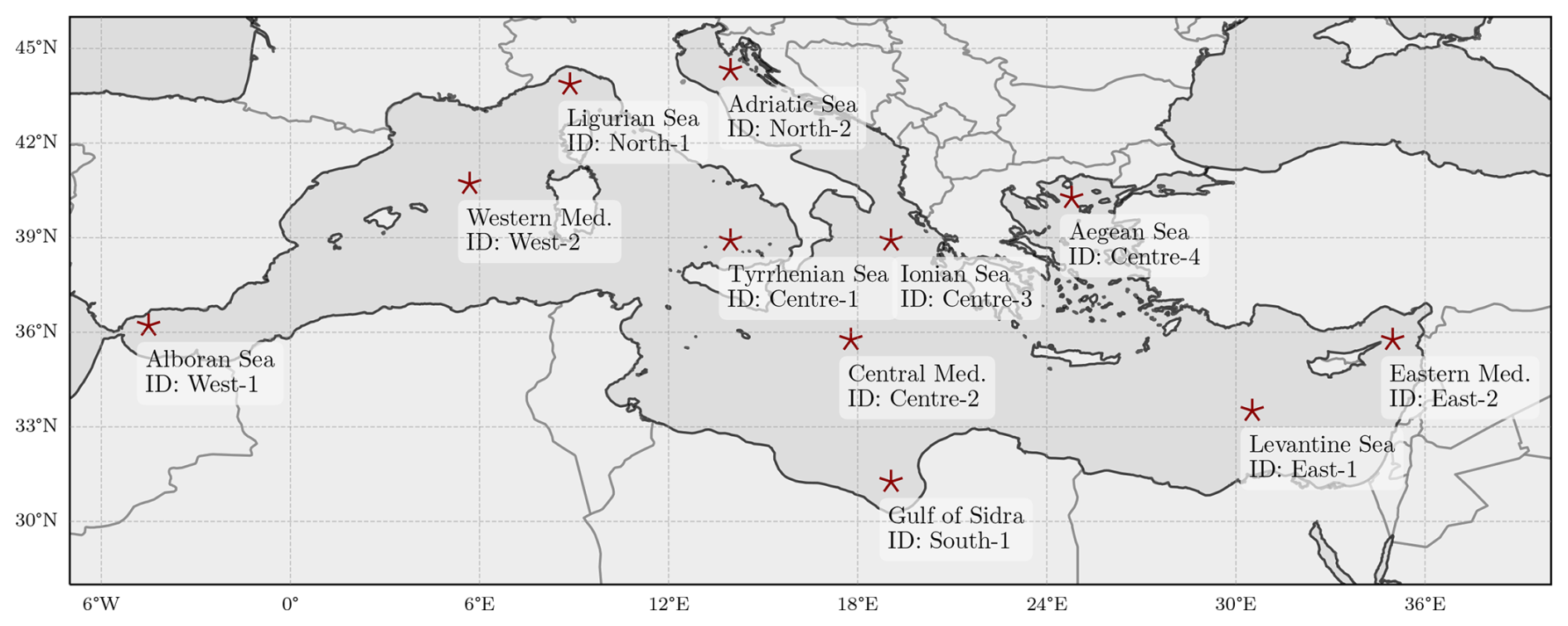
Figure 1 Locations and identification of the analyzed places.

The paper is organized as follows: the “Methods and data” section presents the hindcast and GCM–RCM wave spectrum datasets used in this study, the skill statistics used to quantify the performance of the GCM—RCMs, and the proposed bias correction methodology. The results are presented in the Results section and are discussed in the “Discussion and conclusions” section.

2 Methods and data

2.1 Projections of directional wave spectra

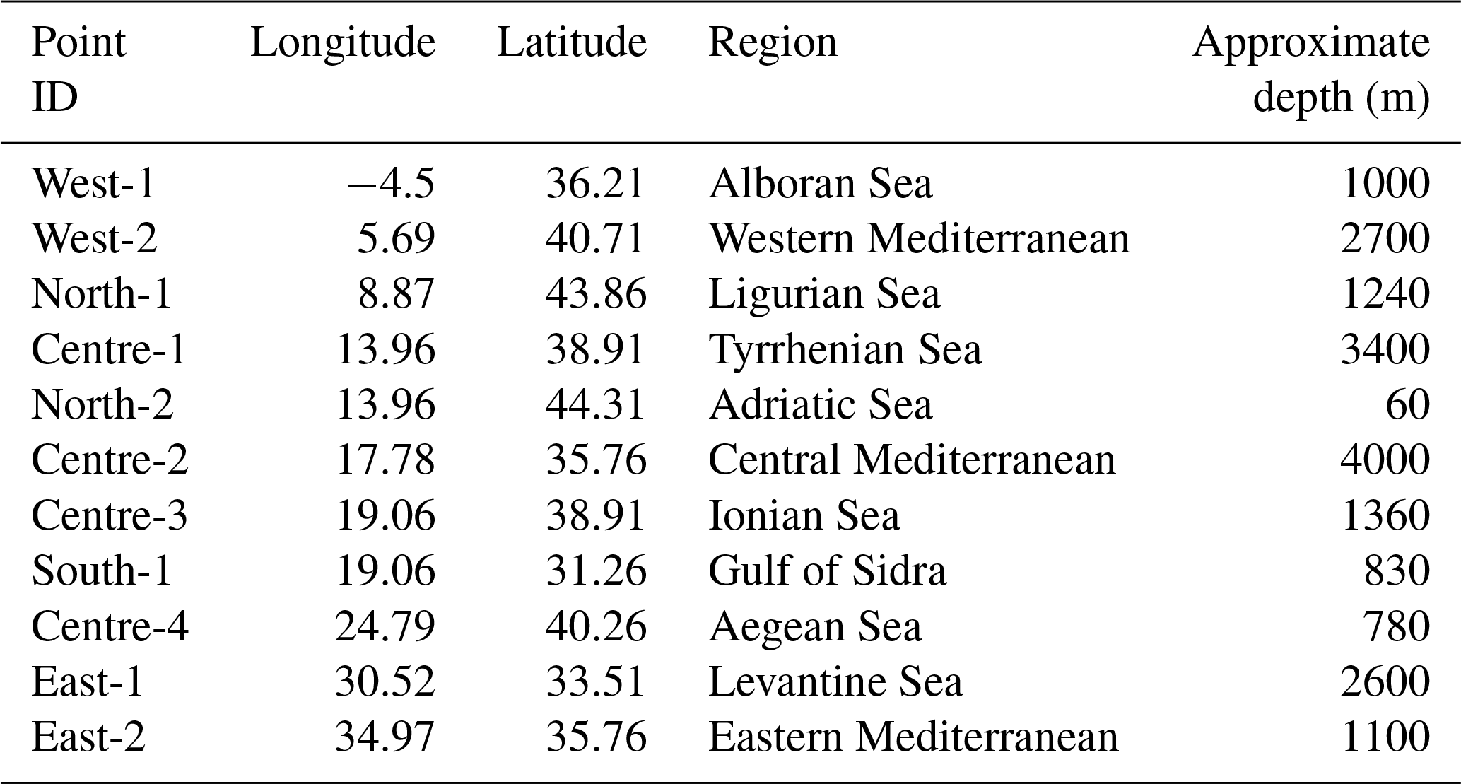
The wave spectrum hindcast used in this work as a proxy for observations was developed by the MeteOcean research group (https://meteocean.science, last access: 11 April 2025) of the University of Genoa (Italy), offering hourly high-resolution wave data from 1979 to 2020 on a regular grid with a resolution of 0.127 by 0.09° in longitude and latitude, respectively, equivalent to ≈10 km and an hourly 2D directional wave spectrum, S(f,θ), for 11 locations in the Mediterranean Sea, as shown in Fig. 1 and Table 1 (Lira-Loarca and Besio, 2022). These locations cover a variety of subbasins within the Mediterranean Sea with distinct regional and local wave dynamics (Lazzari et al., 2012; Besio et al., 2016; Di Biagio et al., 2020; Barbariol et al., 2021). The energy spectrum of each location is divided into 24 directional bins, θ, of 15° each, and 25 frequency bins, f, ranging from approximately 0.07 to 0.66 Hz (or 1.5 to 15 s per period). The hindcast has been developed with the third-generation wave model Wavewatch III (version 5.16) (The WAVEWATCH III:® Development Group, 2019) with the growth and dissipation ST4 source terms (Ardhuin et al., 2010; Rascle and Ardhuin, 2013). The hindcast data have been validated using buoy observations in various locations in the Mediterranean Sea. For more information on the setup and validation, please refer to Mentaschi et al. (2013a, b, 2015) and Besio et al. (2016).

Table 1 Analyzed locations for the different representative regions of the Mediterranean Sea.

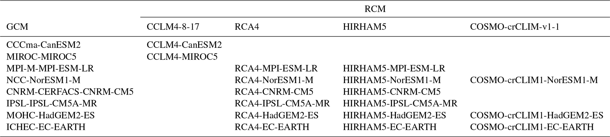
Wave climate projections were obtained with the same WW3 configuration forced by surface wind fields of 17 EURO-CORDEX (Table 2) (Jacob et al., 2014, 2020) models (GCM–RCM combinations) with a temporal resolution of 6 h (Lira-Loarca et al., 2021b; De Leo et al., 2021; Lira-Loarca and Besio, 2022). Wave-integrated parameters and 2D directional spectra for the 11 locations were obtained for each GCM–RCM for the base period (1970–2005) and RCP8.5 scenario (2006–2100). For details of the definition and performance of the different RCMs used in this work, the reader is referred to Strandberg et al. (2014) for the Rossby Centre regional climate model RCA4, Will et al. (2017) for the CLM-Community CCLM4-8-17 model, Christensen et al. (2007) for the Danish Climate Centre regional climate model HIRHAM5, and Leutwyler et al. (2017) for the COSMO-CLM accelerated version COSMO-crCLIM-v1-1.

Table 2 Notation of the used EURO-CORDEX GCM–RCM datasets.

The integrated parameter, wave energy E (m²), is defined as

$$\begin{array}{}\text{(1)}& E=\underset{\mathrm{0}}{\overset{\mathrm{2}\mathit{\pi }}{\int }}\underset{\mathrm{0}}{\overset{\mathrm{\infty }}{\int }}S(f,\mathit{\theta })\mathrm{d}f\mathrm{d}\mathit{\theta },\end{array}$$

where S(f,θ) is the directional wave spectrum.

The contribution of a spectral bin (f, θ) to the directional wave spectrum is defined as

$$\begin{array}{}\text{(2)}& \widehat{S(f,\mathit{\theta })}={\displaystyle \frac{S(f,\mathit{\theta })\mathrm{\Delta }f\mathrm{\Delta }\mathit{\theta }}{E}}.\end{array}$$

2.2 Skill statistics

Skill statistics (bias and RMSE) have been computed for the monthly means and maxima of the directional wave spectral density function between the GCM–RCM data and the hindcast for the common period of 1979–2005 for all the locations and models presented in the tables:

$$\begin{array}{}\text{(3)}& {\displaystyle }\mathrm{bias}={\displaystyle \frac{\mathrm{1}}{N}}\sum _{i=\mathrm{1}}^N\left({\stackrel{\mathrm{‾}}{S(f,\mathit{\theta })}}_{{\mathrm{RCM}}_i}^{\mathrm{baseline}}-{\stackrel{\mathrm{‾}}{S(f,\mathit{\theta })}}_{{\mathrm{hind}}_i}\right),\text{(4)}& {\displaystyle }\mathrm{RMSE}=\sqrt{{\displaystyle \frac{\mathrm{1}}{N}}\sum _{i=\mathrm{1}}^N{\left({\stackrel{\mathrm{‾}}{S(f,\mathit{\theta })}}_{{\mathrm{RCM}}_i}^{\mathrm{baseline}}-{\stackrel{\mathrm{‾}}{S(f,\mathit{\theta })}}_{{\mathrm{hind}}_i}\right)}^{\mathrm{2}}},\end{array}$$

where $\stackrel{\mathrm{‾}}{S(f,\mathit{\theta })}$ is the seasonal mean directional wave spectrum, N is the length of the dataset, and the subscripts and superscripts hind and RCM|baseline correspond to the hindcast and GCM–RCM baseline simulations, respectively, from 1979 to 2005.

2.3 Bias correction

The bias adjustment methodology consists of (i) the conversion of 2D directional wave spectra into wave energy, (ii) the correction of the wave energy 3 h time series using the EGDM-month method, and (iii) the reconstruction of the wave spectrum conserving the initial energy distribution in the frequency and directional bins. The bias correction method proposed in this study, spectral energy Gumbel distribution mapping per month (SEGDM-month), is based on the well-known distribution mapping (also known as the empirical quantile mapping) method (Déqué, 2007) and its adaptation for the correction of the upper tail of the distribution using a Gumbel parametric distribution (Lemos et al., 2020b). To account for the temporal variability of the wave climate, correction is done on a month-by-month basis, correcting each month independently (Lira Loarca et al., 2023). The DM method consists of the adjustment of the distribution of the GCM–RCM projections to match the distribution of the reference historical data:

$$\begin{array}{}\text{(5)}& E^{*}=F_{\mathrm{hind}}^{-\mathrm{1}}\left(F_{\mathrm{RCM}}^{\mathrm{baseline}}\left(E\right)\right),\end{array}$$

where E^* is the bias-adjusted energy, F_ref is the distribution function of the reference historical data (hindcast, 1979–2005), and $F_{\mathrm{RCM}}^{\mathrm{baseline}}$ is the distribution function of each GCM–RCM during the baseline period (1979–2005). The correction is implemented using the empirical cumulative distribution of the datasets for the lower tail and mean body of the distribution (up to the 90th quantile) with linearly distributed quantiles [q₁, q₉₀] every 1 quantile. The upper tail of the distribution (above the 90th quantile) is corrected according to the bias between the parametric Gumbel distributions of the GCM–RCM and reference data.

Once the energy of the integrated parameter, E, has been bias-corrected, the conversion to the directional wave spectrum is done, conserving the relative contribution of each spectral bin (f, θ) to the original wave spectrum ($\widehat{S(f,\mathit{\theta })}$, Eq. 2):

$$\begin{array}{}\text{(6)}& S^{*}(f,\mathit{\theta })=E^{*}\cdot \widehat{S(f,\mathit{\theta })},\end{array}$$

where $S^{*}(f,\mathit{\theta })$ is the bias-corrected directional wave spectrum.

2.4 Performance of bias correction methods

To measure the effectiveness of the bias correction method, simple delta methods have been employed for both the RMSE and bias, defined as

$$\begin{array}{}\text{(7)}& \begin{array}{rl}\mathrm{\Delta }\mathrm{RMSE}& ={\mathrm{RMSE}}^{*}-{\mathrm{RMSE}}^{\mathrm{raw}}\\ & \text{and}\mathrm{\Delta }\mathrm{bias}=\mathrm{|}{\mathrm{Bias}}^{*}\mathrm{|}-\mathrm{|}{\mathrm{Bias}}^{\mathrm{raw}}\mathrm{|},\end{array}\end{array}$$

where the ^* superscript denotes the bias-corrected metric and the raw superscript denotes the raw metric (without bias correction). Therefore, a negative Δ indicates better performance of the bias-adjusted data with respect to the raw data.

2.5 Projected changes in the 3D directional wave spectra

The assessment of future changes in the directional wave spectra under RCP8.5 was done through analysis of seasonal differences between the multimodel ensemble mean and the hindcast wave spectra. For the calculation of the multimodel ensemble mean, a weighted approach is used:

$$\begin{array}{}\text{(8)}& \mathrm{WE}\left[S(f,\mathit{\theta })\right]={\displaystyle \frac{{\sum }_{m=\mathrm{1}}^{N_{\mathrm{m}}}{w}_{\mathrm{m}}\cdot \stackrel{\mathrm{‾}}{S^{*}(f,\mathit{\theta }{)}_{\mathrm{m}}}}{{\sum }_{m=\mathrm{1}}^{N_{\mathrm{m}}}{w}_{\mathrm{m}}}},\end{array}$$

where ${\stackrel{\mathrm{‾}}{S^{*}(f,\mathit{\theta })}}_{\mathrm{m}}$ refers to the bias-adjusted seasonal mean energy density for each GCM–RCM (m=1…17), WE[S(f,θ)] represents the seasonally weighted multimodel ensemble mean, N_m is the number of GCM–RCMs included in the ensemble (N_m=17), and w_m denotes the corresponding weight for each GCM–RCM, which is calculated based on the number of ensemble members forced with the same GCM in relation to N_m. An ordinary arithmetic ensemble mean was also calculated, yielding similar results to the weighted mean approach.

To assess the projected changes in directional wave spectra between the GCM–RCM simulations for the future RCP8.5 and baseline scenarios, the relative change is evaluated between the multimodel ensemble seasonal mean for both periods:

$$\begin{array}{}\text{(9)}& \mathrm{\Delta }S(f,\mathit{\theta })=\mathrm{WE}{\left[S(f,\mathit{\theta })\right]}_{\mathrm{RCP}\mathrm{8.5}}-\mathrm{WE}{\left[S(f,\mathit{\theta })\right]}_{\mathrm{baseline}},\end{array}$$

where ΔS(f,θ) represents the seasonally projected relative change and ${\stackrel{\mathrm{‾}}{S(f,\mathit{\theta })}}_{\mathrm{hind}}$ corresponds to the hindcast seasonal mean.

3 Results

3.1 Performance of bias-adjusted 2D directional wave spectra

The performance of the SEGDM-month bias adjustment method is first assessed through the correction of the integrated wave energy parameter. Figure 2 presents, for each panel, the monthly variability of different energy percentiles for the hindcast (dotted line) and the multimodel ensemble mean (solid line). The ensemble uncertainty is quantified with 1 standard deviation (shaded region). The rows correspond to different locations, while the columns present the raw (left) and bias-adjusted (right) GCM–RCM ensembles. The bias in the wave energy monthly distribution of the raw GCM–RCMs is higher for the higher percentiles, both in magnitude and in the ability to represent the temporal variability. The raw GCM–RCMs presented an overestimation of the upper quantiles for the winter months for North-1 (Ligurian Sea), West-2 (Western Mediterranean) and East-1 (Levantine Sea) and an underestimation for North-2 (Adriatic Sea) and West-1 (Alboran Sea), which are adequately corrected by the SEGDM-month method for all the locations, advocating the use of bias correction methods for integrated parameters. Additionally, the use of the Gumbel distribution for the upper tail allows for a correct characterization of the energy extremes of the bias-corrected GCM–RCM simulations depicted by the higher percentiles.

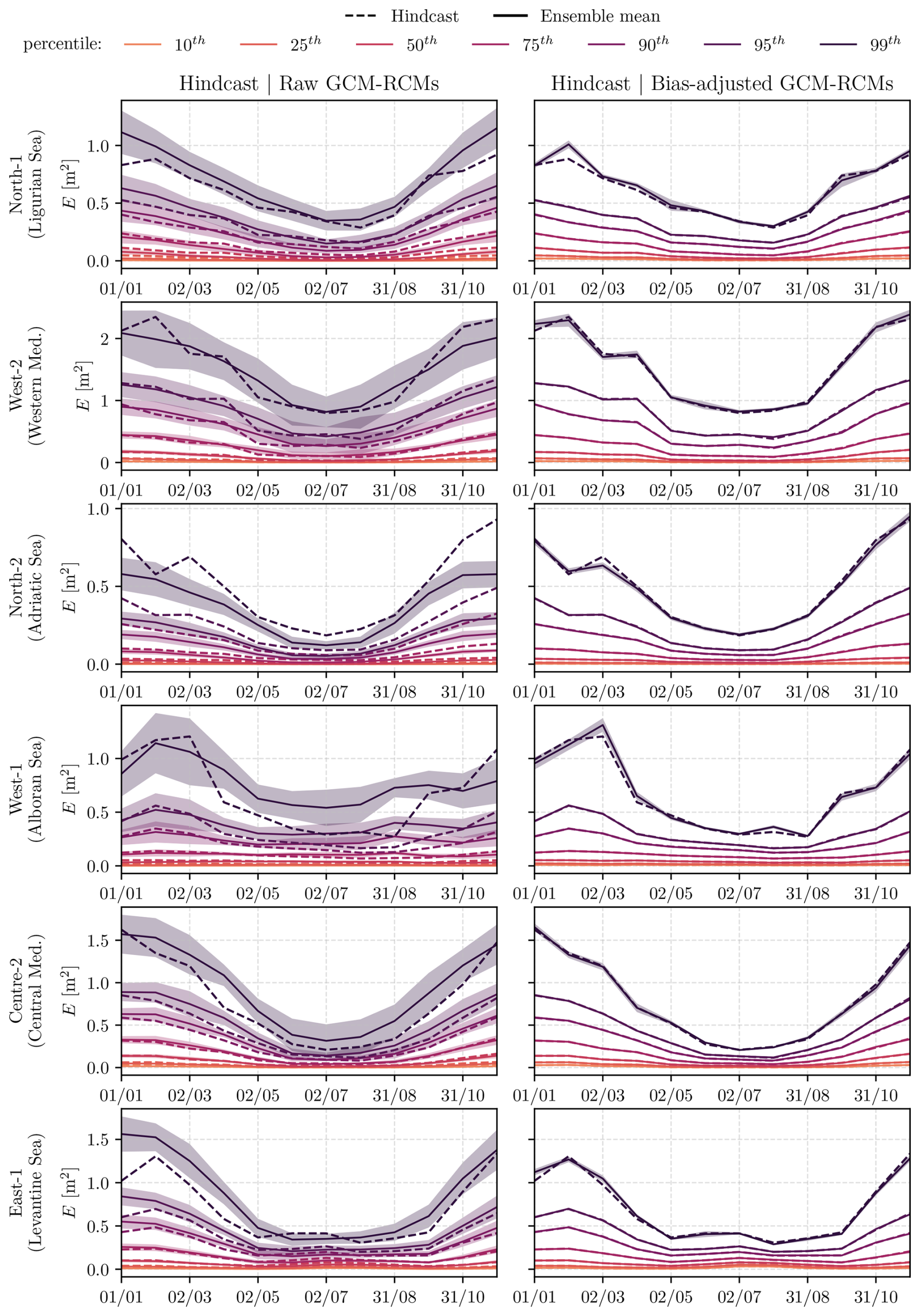
Figure 2 Energy E (m²) monthly percentiles (10th, 25th, 50th, 75th, 90th, 95th, and 99th) for the hindcast (dotted line) and the multimodel ensemble mean (solid line), together with 1 standard deviation from the mean (shaded region) for the baseline period (1979–2005). The rows present the different analyzed locations: North-1 (Ligurian Sea), West-2 (Western Mediterranean), North-2 (Adriatic Sea), West-1 (Alboran Sea), Centre-2 (Central Mediterranean), and East-1 (Levantine Sea). The columns correspond to the raw and bias-adjusted GCM–RCM data.

In order to understand the performance of the GCM–RCMs against the hindcast during the baseline period (1979–2005) for the 2D directional wave spectra, the seasonal bias (Eq. 3) and the RMSE (Eq. 4) of the monthly mean values of the wave spectrum are computed. We present the results of the bias for all of the seasons to analyze the capacity of the method to capture the intra-annual temporal variability of waves. Due to space limitations, we only present the RMSE during winter (December–January–February or DJF), where the highest wave energy systems are expected. The remaining seasonal RMSE results are presented in the Supplement.

Figure 3 presents, for each analyzed location, the winter (DJF) mean of the wave spectrum monthly means for the hindcast (left), the bias between the hindcast and the raw GCM–RCM (middle), and the difference in the bias ΔBias (Eq. 7) for the bias-adjusted GCM–RCM (right). For each location, the worst-performing GCM–RCM is presented. Figures 4 to 7 present, for the monthly means, the winter RMSE and the spring, summer, and fall biases.

For the winter bias of the monthly means (Fig. 3), the results show a systematic underestimation for the most energetic bins for the raw GCM–RCM spectra in the West-1 (Alboran Sea), West-2 (Western Mediterranean), North-2 (Adriatic Sea), and Centre-4 (Aegean Sea) locations, while the remaining locations present an overestimation of the most energetic bins which correspond to the swell system. A negative ΔBias indicates an improvement in the performance of the GCM–RCM wave spectra with respect to the hindcast due to bias correction. It can be observed that the bias, in the most energetic systems, is reduced for all of the locations, except for North-2 (Adriatic Sea) and Centre-4 (Aegean Sea), where no noticeable changes are observed, and Centre-3 (Ionian Sea), where the most energetic system (SE–SW) presents decreases for the southwesterly waves and increases for the southeasterly waves. It can also be observed that, for some locations, the use of the bias correction method leads to an increase in the bias for the least energetic systems, as observed for West-1 (Alboran Sea), Centre-3 (Ionian Sea), North-2 (Adriatic Sea), West-2 (Western Mediterranean), and Centre-4 (Aegean Sea), where increases in the biases range from 0.002 to 0.005 m² s per degree but the integrated wave energy is conserved in the hindcast distribution.

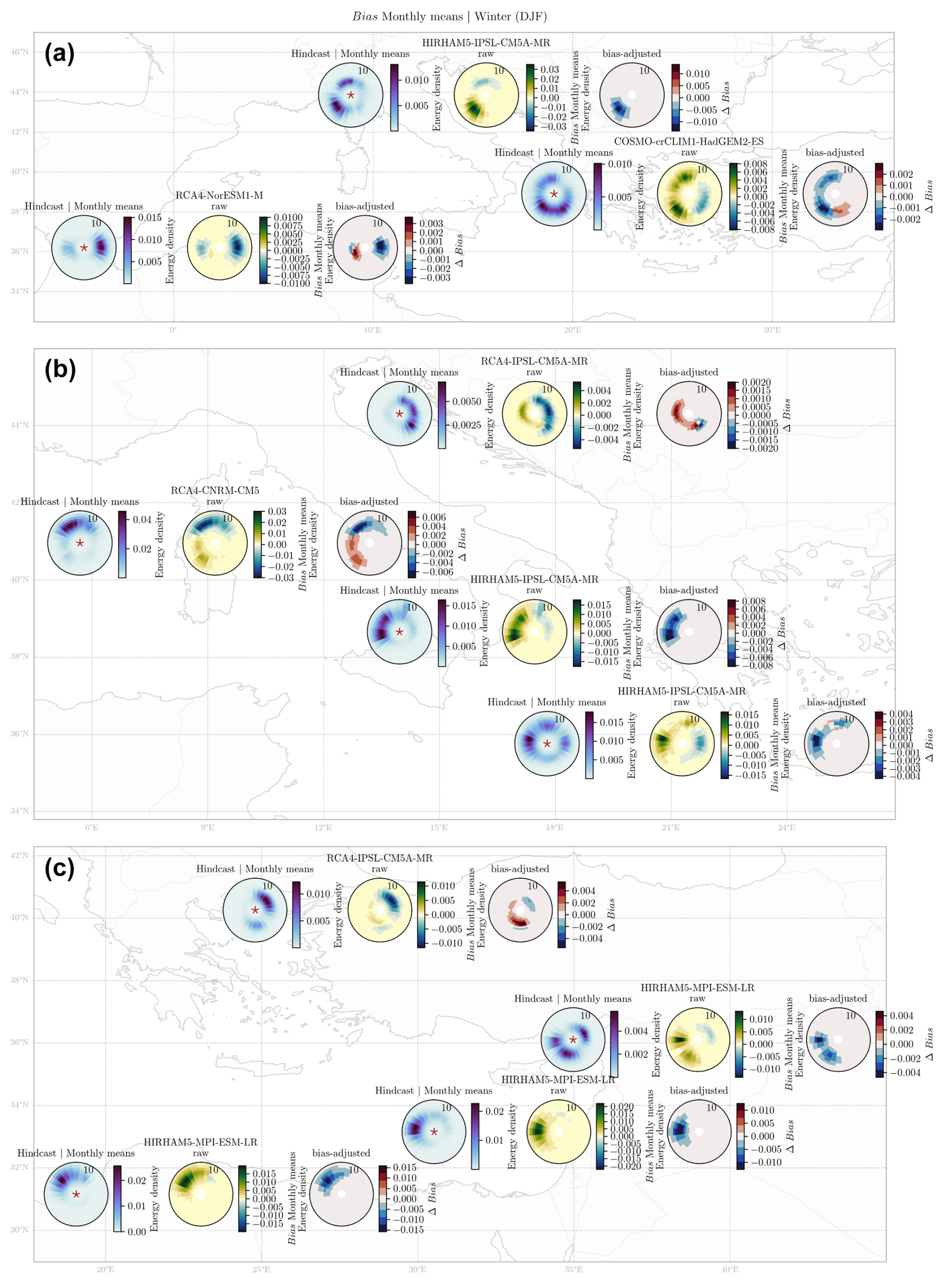
Figure 3 Results of the monthly mean 2D spectra averaged over the winter (DJF; m² s per degree). For each location there are the hindcast wave spectrum (left panel), bias between the raw worst-performing GCM–RCM and hindcast (middle panel), and ΔBias between the bias-adjusted Bias^* and the raw bias. The star in the hindcast or left panel represents the locations of the points corresponding to Fig. 1.

Regarding the winter mean of the RMSE of the monthly means depicted in Fig. 4, it can be observed that the use of the bias correction method presented in this work leads to increased error in the North-2 (Adriatic Sea) and Centre-4 (Aegean Sea) locations for the winter RMSE, although different behaviors are observed for the remaining seasons (Supplement). Indeed, the North-2 (Adriatic Sea) and Centre-4 (Aegean Sea) locations are characterized by local-scale phenomena that might not be captured entirely by GCM–RCM resolution (Lira-Loarca and Besio, 2022). In the case of West-1 (Alboran Sea), Centre-3 (Ionian Sea), and West-2 (Western Mediterranean), where the bias presented a decrease in performance for the bias-adjusted low-energy systems, the RMSE depicts an increase in performance for all of the bins. This is due to the calculation of the RMSE for wave spectrum errors, which exhibit values less than 1, and upon squaring them their magnitudes diminish further, leading to smaller errors for the RMSE with respect to bias. For the remaining locations, the application of the bias adjustment techniques leads to an improved performance of the data for all of the spectral bins.

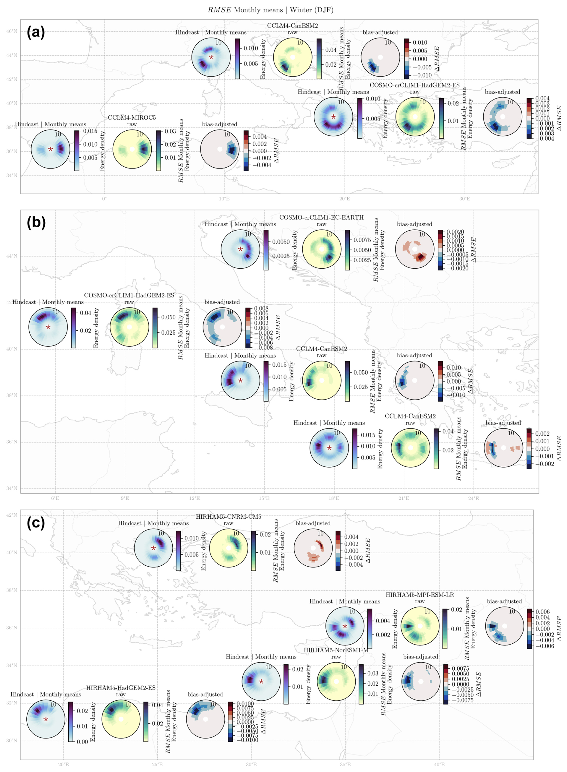
Figure 4 Results of the monthly mean 2D spectra averaged over winter (DJF; m² s per degree). For each location: hindcast wave spectrum (left panel), RMSE between the raw worst-performing GCM–RCM and the hindcast (middle), and the ΔRMSE between the bias-adjusted RMSE^* and the raw RMSE.

Regarding the bias correction results for the remaining seasons, Figs. 5–7 present the bias of the monthly means for spring, summer, and fall, respectively. Similar behavior is depicted for all of the seasons, where the bias correction leads to improvement in performance for the most energetic wave systems. Spring (March–April–May or MAM, Fig. 5) and fall (September–October–November or SON, Fig. 7) present a similar spectrum distribution for hindcasts to winter. As described previously, for the winter monthly means, the bias correction led to an increase in errors for some locations, whereas in the case of spring and fall the bias correction leads to a general improvement in the performance for all of the locations. For example, the West-2 (Western Mediterranean), West-1 (Alboran Sea), and Centre-4 (Aegean Sea) locations presented an increase in errors in the least energetic systems after the bias correction during winter, but this is not the case for spring and fall, when there was a general improvement in all of the systems in these locations. Although the hindcast energy density magnitude for spring and fall is smaller than in winter, decreases in bias of around 50 % are observed for all of the locations and systems. Similar behavior is depicted for the summer mean bias (Fig. 6), where the bias correction leads to an improvement in performance in almost all of the locations, with the exception of North-2 (Adriatic Sea) and East-1 (Levantine Sea) for the low-energy bins. Therefore, the use of the monthly EGQM method presented in this work captures the intra-annual temporal variability of the spectra and correctly adjusts the bias for all of the seasons.

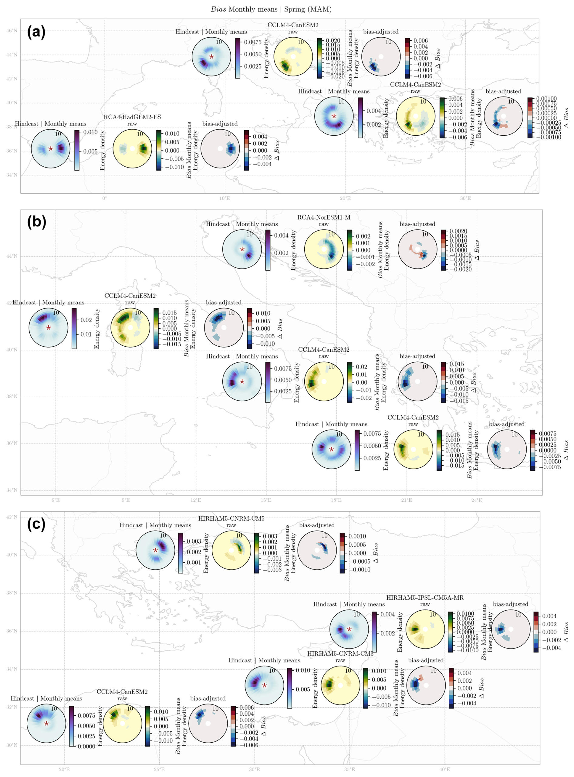
Figure 5 Monthly mean 2D spectra averaged over the spring (MAM; m² s per degree). For each location: hindcast wave spectrum (a), bias between the raw worst-performing GCM–RCM and the hindcast (b), and ΔBias between the bias-adjusted Bias^* and the raw bias (c).

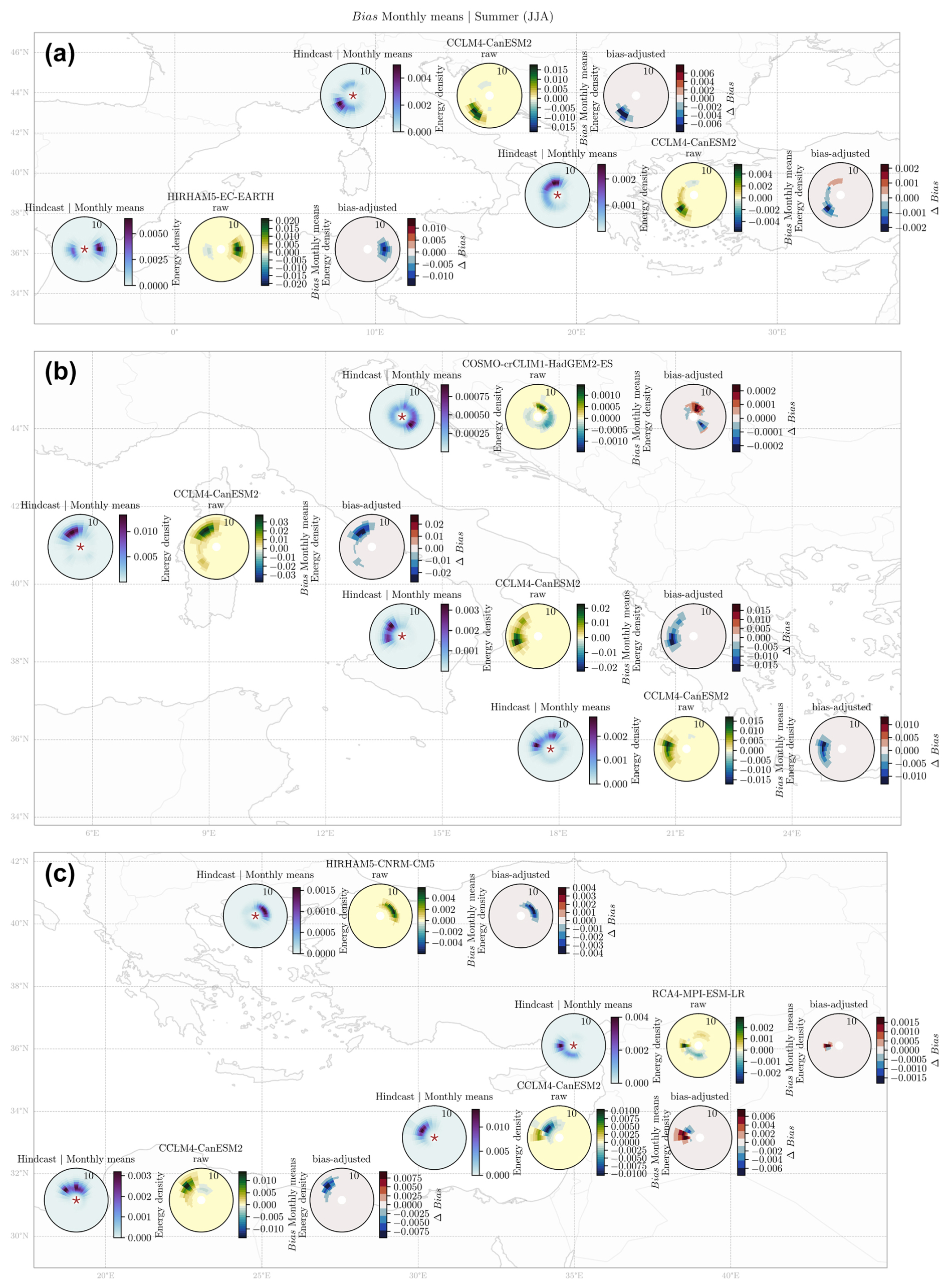
Figure 6 Monthly mean 2D spectra averaged over the summer (JJA; m² s per degree). For each location: hindcast wave spectrum (a), bias between the raw worst-performing GCM–RCM and the hindcast (b), and ΔBias between the bias-adjusted Bias^* and the raw bias (c).

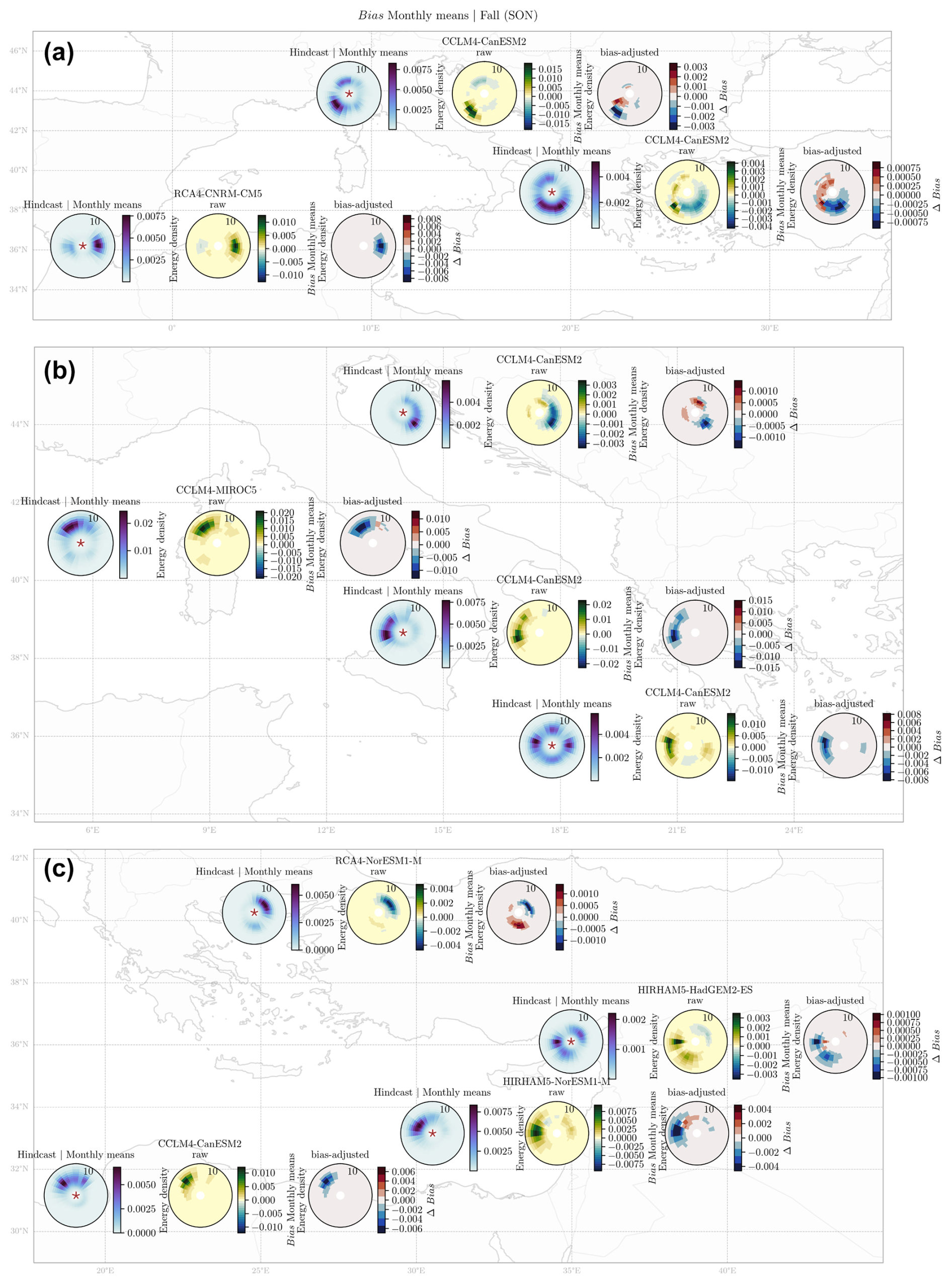
Figure 7 Monthly mean 2D spectra averaged over the fall (SON; m² s per degree). For each location: hindcast wave spectrum (a), bias between the raw worst-performing GCM–RCM and the hindcast (b), and ΔBias between the bias-adjusted Bias^* and the raw bias (c).

3.2 Future changes in 2D wave spectra in RCP8.5

Regarding future changes in the RCP8.5 climate change scenario, Figs. 8 and 9 present projected changes for future monthly means and maxima, respectively, during spring (MAM). The seasonal monthly maxima are the average of the monthly maxima of the 2D directional wave spectra during the analyzed period, when the selection of the monthly maximum spectra is done, corresponding to the point in time of the maximum wave energy. The remaining seasons are included in the Supplement. Each figure presents, for each location, the spring (MAM) mean of the wave spectrum monthly means or maxima for the hindcast and the multimodel ensemble mean during the baseline period (1979–2005) and the differences between the multimodel ensemble mean for the mid-century (2034–2060) and the end of the century (2074–2100) with respect to the baseline period. The stippling indicates regions where at least 80 % of the models agree with the sign of the change. The lack of stippling indicates low model agreement (less than 80 %).

Regarding the projected changes in the monthly mean wave spectra (Fig. 8), it can be observed that West-1 (Alboran Sea) presents similar 2D spectra between the hindcast and the ensemble mean for baseline conditions for the most energetic easterly waves, with robust projected increases for both periods leading to a projected change in bimodal hindcast spectra to predominantly unimodal easterly swells. For the North-1 (Ligurian Sea) location, it can be noted that the ensemble presents higher spectrum values with respect to hindcasts for the main southwesterly system, and the projections indicate different behaviors in this system depending on the frequency, although without model agreement. The Centre-3 (Ionian Sea) location presents projected decreases for the more energetic southeasterly wind at the lower frequencies for both periods and an increase for the higher frequencies.

The West-2 (Western Mediterranean) location depicts future behavior in which the main hindcast NW–N swell system presents an increase in both periods, although without model agreement, and a robust decrease in the less energetic southwesterly waves. These were not noticeable in the hindcast. This behavior is also observed in the North-2 (Adriatic Sea) location, where a robust increase in the southeasterly waves is depicted for both periods. On the other hand, different behavior is observed for the remaining locations, where the projected changes indicate a robust decrease in the most energetic swell system. For the Centre-2 (Central Mediterranean) and South-1 (Gulf of Sidra) locations, an increase can be observed for the less energetic systems, although without model agreement.

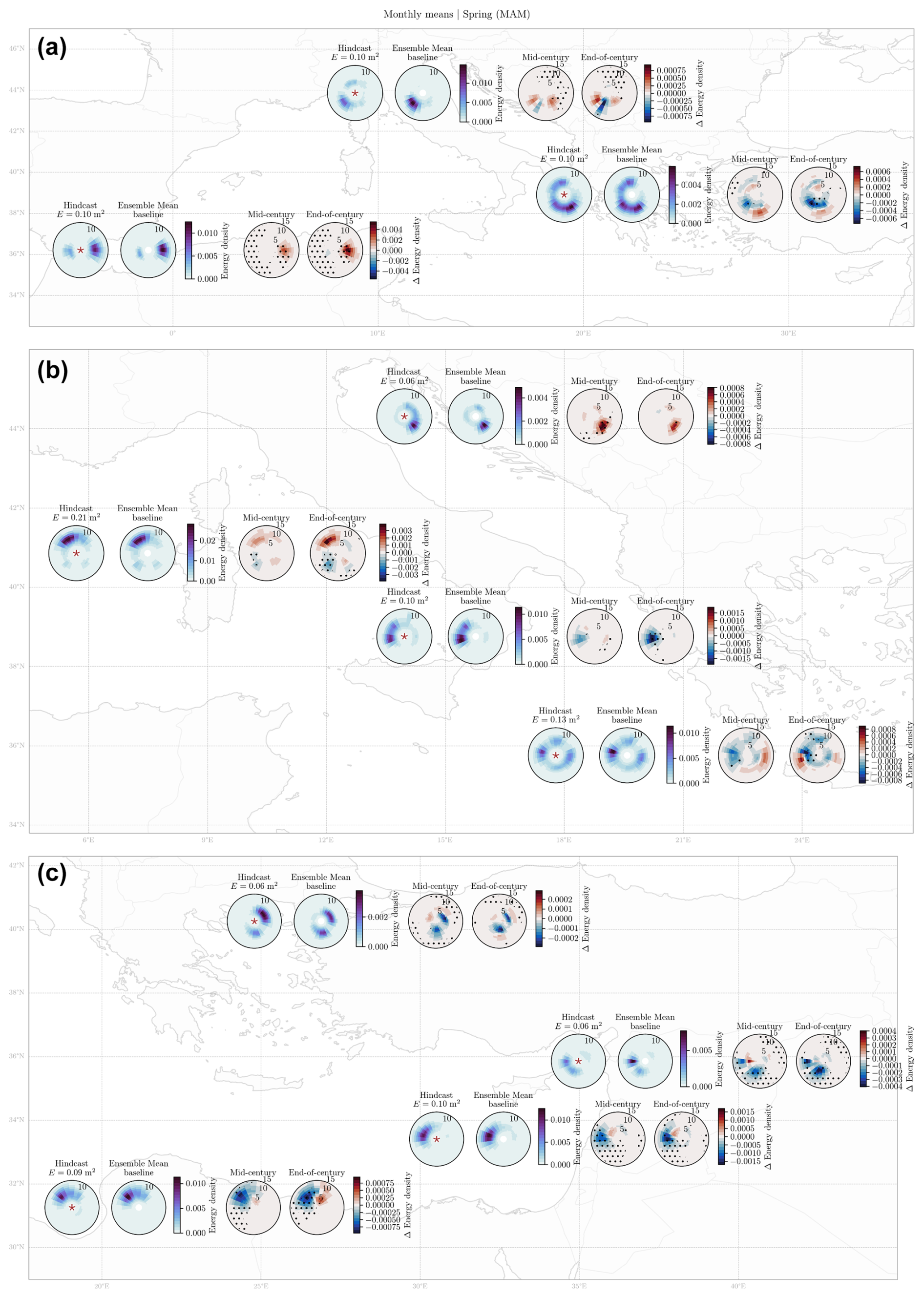
Figure 8 Spring (MAM) seasonal mean 2D spectra (m² s per degree). For each location: hindcast wave spectrum, ensemble mean for baseline conditions, and changes between the multimodel bias-adjusted ensemble mean with respect to the baseline period for mid-century (2034–2060) and end-of-century conditions (2074–2100), for all the analyzed locations in the Mediterranean Sea. Stippling indicates regions where at least 80 % of the models agree on the sign of the change. A lack of stippling indicates low model agreement (less than 80 %). The star in the hindcast or left panel represents the locations of the points corresponding to Fig. 1.

Regarding the projected changes in the monthly maximum wave spectra during spring (Fig. 9), a projected increase, without model agreement, is observed in the main southeasterly swell system of North-1 (Ligurian Sea), leading to more intense southwesterly storm events. This behavior is also observed for the West-1 (Alboran Sea), North-2 (Adriatic Sea), and West-2 (Western Mediterranean) locations, where an increase in the main system is observed for future conditions. Centre-3 (Ionian Sea) provides different results, with a main SE–SW hindcast swell system that depicts robust projected decreases for NW waves and increases for SW–W waves for the higher frequencies, leading to a more bimodal or unimodal behavior, in contrast to the hindcast multimodal extreme wave spectra. For the Centre-2 (Central Mediterranean) and Centre-4 (Aegean Sea) locations, different behaviors are observed for the varying frequencies and directions of the spectra, with no definite results on the future behavior of the systems. Finally, Centre-1 (Tyrrhenian Sea), South-1 (Gulf of Sidra), East-1 (Levantine Sea), and East-2 (Eastern Mediterranean) present robust decreases in the main energetic systems for both future periods. It can be highlighted that, for all of the locations, the ensemble mean under baseline conditions provides an accurate representation of the hindcast wave spectra, highlighting the performance of the SEGDM-month method and the energy distribution provided by the GCM–RCMs.

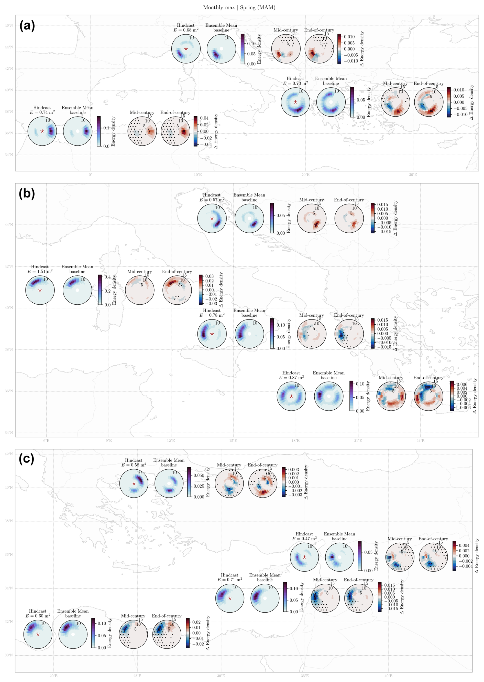
Figure 9 Monthly maximum 2D spectra averaged over spring (MAM; m² s per degree). For each location: hindcast wave spectrum, ensemble mean for the baseline, and changes between the multimodel bias-adjusted ensemble mean with respect to the baseline period for mid-century (2034–2060) and end-of-century conditions (2074–2100), for all of the analyzed locations in the Mediterranean Sea. The stippling indicates regions where at least 80 % of the models agree on the sign of the change. A lack of stippling indicates low model agreement (less than 80 %).

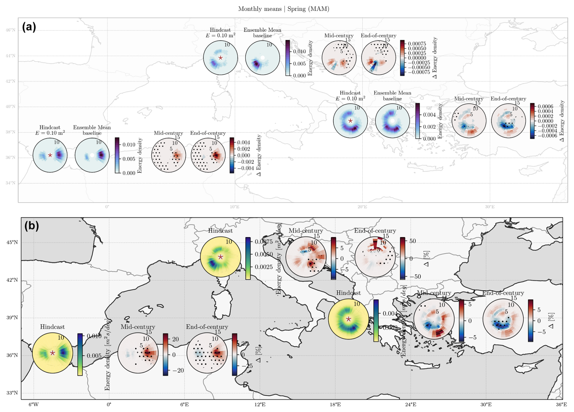
Figure 10 Mean directional spectra for spring (March, April, and May). Panel (a) is extracted from Fig. 8, indicating the hindcast wave spectrum, ensemble mean for baseline conditions (1979–2005), and changes between the multimodel bias-adjusted ensemble mean with respect to the baseline period in RCP8.5 for mid-century (2034–2060) and end-of-century conditions (2074–2100). Panel (b) is extracted from Fig. 5 of Lira-Loarca and Besio (2022), representing, for each location, the hindcast data and projected percent change for the multimodel ensemble for the middle of the century and the end of the century. In both panels, the stippling indicates regions where at least 80 % of the models agree on the sign of the change.

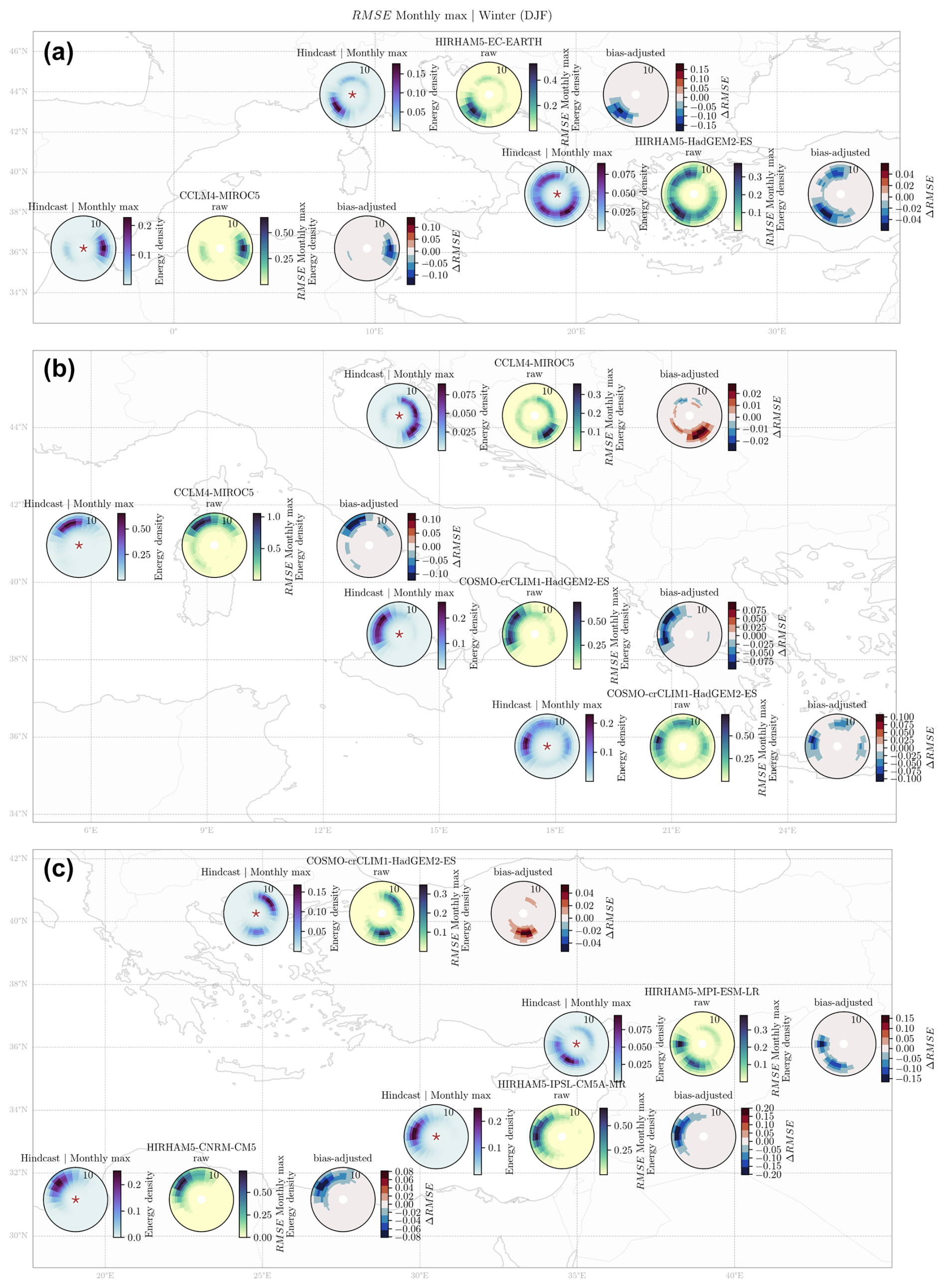
Figure 11 Results of the monthly maximum 2D spectra averaged over the winter (DJF). For each location: hindcast wave spectrum (a), RMSE between the raw worst-performing GCM–RCM and the hindcast (b), and ΔRMSE between the bias-adjusted RMSE^* and the raw RMSE (c).

4 Discussion and conclusions

This work presents the application of a novel bias correction technique designed for 2D wave spectra by means of the conservation of the integrated wave energy. Although the application of bias correction techniques is extended among hydrological impact studies and the need for and benefits of wave projections have been highlighted by recent studies applied to integrated wave parameters (Lemos et al., 2020b, a; Lira Loarca et al., 2023), the correction of the 2D directional wave spectra using the integral frequency and directional dimensions remains unexplored (Lobeto et al., 2021a; Lira-Loarca and Besio, 2022). Lira-Loarca and Besio (2022) performed bias adjustment by applying the widespread delta method to the seasonal mean statistics of the wave spectra on a bin-by-bin basis, which did not allow for a reconstruction of the complete time series of spectra and led to a lack of energy conservation within the bias-corrected spectra, and it is not flexible in allowing possible future directional and frequency shifts that were not present under the historical baseline conditions. This study is the first attempt to perform bias adjustment of 2D directional wave spectra, not bin by bin, but in an integrated frequency–direction manner. SEGDM-month works on the correction of the integrated wave energy parameter, taking into account the intra-annual variability and allowing energy distribution in the frequency and direction following the climate signal of the GCM–RCM. The choice to maintain the energy distribution given by the original GCM–RCM allows one to explore the possible shifts in direction and periods given by the global climate models not present under historical conditions. In order to compare the possible implications of the bias correction technique for the assessment of future changes, Fig. 10 presents the mean directional spectra for spring (March, April, and May) obtained by Lira-Loarca and Besio (2022) and the ones presented in this paper. It can be observed that, for the West-1 (Alboran Sea) and Centre-3 (Ionian Sea) locations, both the delta and SEGDM-month methods lead to a similar distribution for changes under mid-century conditions, whereas some changes present in the delta method for the end of the century, such as a robust decrease for the western system in West-1 (Alboran Sea) and increases in the easterly directions for Centre-3 (Ionian Sea), are not present in the SEGDM-month method. On the other hand, for North-1 (Ligurian Sea), different, almost contrary results are obtained by the two methods, where an increase in northerly swells was depicted for the end of the century for the delta method that was not present in SEGDM-month, where both decreases and increases are obtained for the main southwesterly system. Therefore, the choice of bias correction method is crucial for a correct assessment of future changes and, consequently, coastal and marine adaptation and resilience strategies. This work highlights the need to consider possible future shifts in the 2D wave spectra for local impact assessments instead of only considering changes in integrated parameters such as significant wave height and mean wave direction.

The SEGDM-month bias correction method presented in this work allows correction of the full time series of the 2D directional wave spectra and better characterization of extremes due to the fit of a Gumbel distribution to the upper tail of the energy distribution, which, to the best of the authors' knowledge, has not been addressed in previous studies. Figure 11 presents, for each location analyzed, the winter (DJF) mean of the wave spectrum monthly maxima for the hindcast (left), the RMSE between the hindcast and raw GCM–RCM (middle), and the difference in the bias ΔRMSE (Eq. 7) for the bias-adjusted GCM–RCM (right). For each location, the worst-performing GCM–RCM is presented. It can be seen that, for all of the locations except North-2 (Adriatic Sea) and Centre-4 (Aegean Sea), there is an improvement in the performance of the baseline simulation of GCM–RCM, highlighting the ability of the proposed method to adjust the biases for different 2D spectrum distributions. Following these results, further studies could focus on multivariate bias correction techniques, although care must be taken to allow possible bin shifts given by future climate signals and to account for the wave temporal variability and extreme events.

This study focuses on bias correction and future changes in directional wave spectra, relying exclusively on the high-emission, business-as-usual scenario RCP8.5. This approach provides insights into future changes and risks in a plausible yet pessimistic scenario. However, the use of a single scenario is recognized as a limitation for developing mitigation strategies, as incorporating multiple emission and mitigation pathways would enable a more comprehensive assessment of projected wave climate changes. The decision to use RCP8.5 only was driven by constraints on computational resources and data storage, which are necessary for simulating a large ensemble of GCM–RCM wave climate projections. Additionally, within EURO-CORDEX, the availability of GCM–RCM forcings is significantly greater for RCP8.5 than for other scenarios. Future research should address this limitation by incorporating a wider range of emission and mitigation scenarios, ensuring an optimal balance between scenarios, GCMs, and RCMs.

This work represents a step forward in the analysis of 2D wave spectrum projections, which allows identification of changes in individual wave systems and a more detailed and realistic assessment of future wave changes with respect to the use of integrated wave parameters where mean or peak values do not allow for full understanding of the complexities of wave climate dynamics.