Hydrographic section along 55° E in the Indian and Southern oceans

A hydrographic section along 55° E, south of 30° S, was visited from December 2019 to January 2020 as the first occupation under the Global Ocean Ship-based Hydrographic Investigations Program. The water column was measured from the sea surface to 10 dbar above the bottom with eddy-resolving station spacings and state-of-the-art accuracy. The upper profile was characterised by a conspicuous front between 42.5 and 43° S and a cold-core eddy at 39° S. The front was identified as the confluence of Subtropical and Subantarctic fronts. The Agulhas Return Current front was found at 41.6° S. When combined with the section north of 30° S observed in 2018, another subsurface front was found in dissolved oxygen around 28° S at depths of 1500 to 3000 dbar. In the eastern Weddell–Enderby Abyssal Plain, no obvious large-scale flow was observed at depths greater than 3000 dbar. We used transient tracers to estimate isopycnal diffusivity there to be 72±16 m² s⁻¹. Antarctic Bottom Water in the basin consisted of water masses originating from the Cape Darnley region (0 %–35 %) and Weddell Sea Deep Water (5 %–75 %) diluted by Lower Circumpolar Deep Water above. These snapshot observations not only confirm hydrographic features reported earlier in the Madagascar and Crozet basins, but also describe the diffusive nature of the deep to bottom circulation in the Weddell–Enderby Abyssal Plain.

1 Introduction

Antarctic Bottom Water (AABW) produced around Antarctica spreads equatorward mainly along the western boundaries of the ocean basins. For this reason, hydrographic sections revealing the deep water masses along 50 or 60° E in the Indian Ocean have often been discussed in the context of global-scale circulation (e.g. Johnson, 2008; Mantyla and Reid, 1983). Nevertheless, synoptic hydrographic observations of these sections (Warren, 1978; Park et al., 1993) are rare mainly because of logistical difficulties. The GO-SHIP (Global Ocean Ship-based Hydrographic Investigations Program) section I07S is one of these sections and was occupied for the first time in the austral summer of 2019/20. It extends the existing section (I07N; equatorward of 30° S) to Cape Ann, the northernmost point in East Antarctica (Fig. 1).

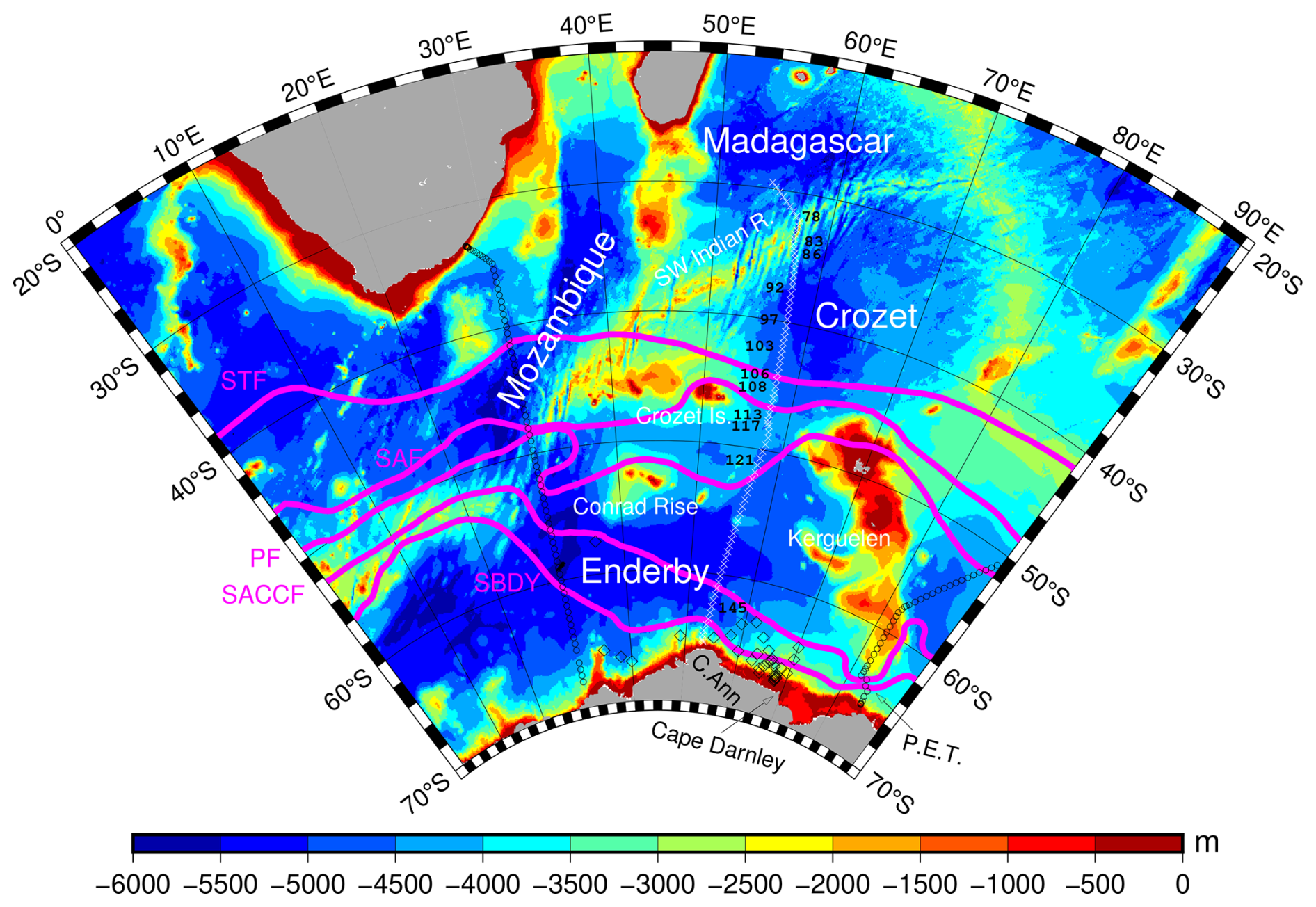
Figure 1 ETOPO5 bathymetry (colour scale) with basin names and topographic features, C.Ann (Cape Ann), and P.E.T. (Princess Elizabeth Trough). The white crosses between 50 and 60° E indicate the I07S section, the black circles at 30° E indicate the I06S section, and those between 80 and 90° E indicate the I08S section (stations occupied in 2007). Selected stations along the I07S section are labelled. The southernmost station is 153. The diamonds near the coast of Antarctica are R/V Hakuho (KH) cruise stations. The magenta lines show the climatological positions of the five major fronts as defined by Orsi et al. (1995): Subtropical Front (STF), Subantarctic Front (SAF), Polar Front (PF), Southern Antarctic Circumpolar Current Front (SACCF), and Southern Boundary (SBDY).

The section follows the approximate flow path of AABW and also crosses the Antarctic Circumpolar Current (ACC). When the ACC, which manifests itself as a bundle of fronts, flows between or over topographic features, mesoscale eddies are produced. The section crosses these fronts and eddies (Fig. 1). These fronts as well as water masses at shallow and intermediate depths have been extensively studied in a series of cruises by Young-Hyang Park (Park et al., 1991, 1993; Park and Gambéroni, 1997; Park et al., 1998) and by later cruises (e.g. Meijers et al., 2010; Williams et al., 2010; Jullion et al., 2014; Ryan et al., 2016). In contrast, the deep circulation within the Weddell–Enderby Abyssal Plain has received limited attention. In this paper, for convenience, we call the eastern part of the Abyssal Plain the “Enderby Basin”. The northern limb of the gyral circulation within the Enderby Basin is an eastward flow along the southern flank of the Southwest Indian Ridge; Gordon and Huber (1984) called this flow the “Weddell cold regime” because the water mass is mixed with cold winter water produced along the coastal shelves of the Weddell Sea. This cold water mixes with relatively warm water carried by the ACC to form the “Weddell warm regime”, which flows westward as the southern limb of the Weddell Gyre. The eastern boundary of the Weddell Gyre has not been clearly defined by observation data. Direct measurement of velocity by a lowered acoustic Doppler current profiler (Meijers et al., 2010) suggests that the boundary is close to 40° E. Jullion et al. (2014) used a box inverse model to estimate transports across the I06S section (30° E). They found the zonal transport in deep to bottom layers to be mostly eastward along the southern flank of the Southwest Indian Ridge, but it includes both eastward and westward components in the interior of the Enderby Basin. Further south near the coast, the transport is dominated by a westward flow along the Antarctic Slope Front. It is not clear how these structures extend eastward to the I07S section at 55° E. Here, we examine the deep circulation in the Enderby Basin as revealed by hydrographic data collected along the section where it passes through the basin.

As the subtropical frontal jet of the ACC negotiates the Southwest Indian Ridge around 45° E, 40° S, vigorous eddies are produced to the leeward side over the Crozet Basin (Fig. 2). At 1000 dbar depth, eddy activity is also seen at around 30° E, 50° S, and its effects extend to the Enderby Basin to the leeward side. The difference between the surface and 1000 dbar might be attributable to the choice of contour values, to weaker stratification over the Enderby Basin, or to both.

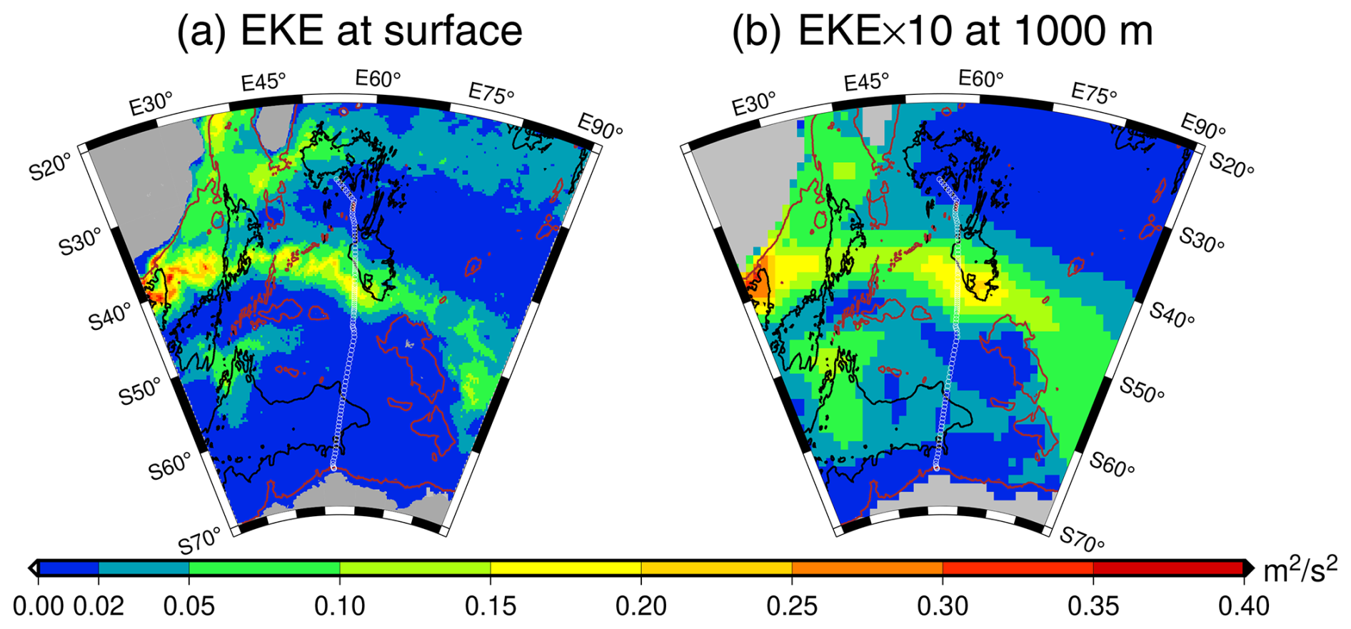
Figure 2 Eddy kinetic energy (EKE) at the surface (a) and at 1000 dbar depth (b). Note that the 1000 dbar EKE (b) is multiplied by a factor of 10. The surface EKE was estimated from geostrophic velocity anomalies of the altimetry data on a 0.25° grid. Values at 1000 dbar were estimated from the Scripps Argo float drift data on a 1° grid. The mean field was defined as the spatial and temporal average within a circle of radius 300 km with the centre at the grid point. See Katsumata (2017) for details of the EKE calculation at 1000 dbar. Black and brown bathymetry contours indicate 5000 and 2000 m depth, respectively.

Our analysis shows that, because of these eddies, the deep circulation in the Enderby Basin is diffusive (see Sect. 4.1).

Further south along the Antarctic coast, the I07S section crosses the westward-flowing Antarctic Slope Front (not shown in Fig. 1). Considering data from a transient tracer section across the Weddell Gyre, Meredith et al. (2000) predicted the existence of a deep water source at around 75° E, upstream of the Antarctic Slope Front. Later, Ohshima et al. (2013) identified a deep water source near Cape Darnley (Fig. 1). Turning to numerical simulations, we find that a tracer (“brine”) release experiment by Kusahara et al. (2017) showed that the bottom water in the Enderby Basin is mostly from the Cape Darnley polynya. Initially, the tracer spread westward over the continental shelf; it then circulates the Weddell Gyre before continuing equatorward into the Crozet Basin. There also appeared to be a direct path from Cape Darnley to the Crozet Basin (Fig. 10d of Kusahara et al., 2017). The direct spread of fresh Cape Darnley Bottom Water (CDBW) to the Enderby Basin is consistent with the result of mixing budget analyses using near-bottom hydrographic data by Aoki et al. (2020a) and Gao et al. (2022). This behaviour of the bottom water is also consistent with the observed property distribution (Fig. 8b of Orsi et al., 1999); the temperature–salinity characteristics at bottom water densities was much fresher within the longitude band of 30 to 60° E than those within 60 to 90° E. In Sect. 4.2, we estimate the mixing ratio of Cape Darnley Bottom Water and Weddell Sea Deep Water.

This paper discusses three distinct topics derived from one data set:

1. overview of the hydrographic features with a focus on conspicuous fronts (Sect. 3)

2. isopycnal diffusivity that quantifies the diffusive nature of the circulation in the deep Enderby Basin (Sect. 4.1)

3. composition of AABW in the Enderby Basin (Sect. 4.2).

These three topics are preceded by a data description (Sect. 2) and followed by a conclusion (Sect. 5). The three topics are only loosely interdependent.

Eleven stations were reoccupations of previous stations at which high-precision hydrographic data had been obtained. The observed changes since the previous occupation are summarised in the Appendix.

2 Data

The primary data used here are from conductivity, temperature, and depth profiler (CTD) and bottle measurements made on board R/V Mirai during the cruise from 31 December 2019 (first station, 70, at 29.5° S) to 22 January 2020 (last station, 153, near seasonal ice edge at 65.3° S), nominally along 55° E (Uchida et al., 2021). The station numbers used in this work are the original station numbers found in the summary file (https://cchdo.ucsd.edu/data/14953/49NZ20191229su.txt, last access: 10 February 2025). By using the reference thermometer (SBE35) and bottle data, the CTD data comply with the GO-SHIP standard accuracies of 0.002 °C (temperature), 0.002 g kg⁻¹ (salinity), and 1 % (dissolved oxygen) (Hood, 2010). Standard methods were used for bottle data analysis: the Winkler method for oxygen (0.15 % uncertainty), the optical methods by auto-analyser for nutrients utilising certified materials (mean coefficient of variance less than 0.2 % for nitrate, silicate, and phosphate), and chromatography for transient tracers (precision for duplicate sampling less than 0.009 pmol kg⁻¹ for CFC12 and 0.014 fmol kg⁻¹ for SF₆). The details are found in Uchida et al. (2021). Expendable CTDs (XCTDs) were used for two purposes: one was to attempt resolving frontal structures and the other was to replace CTD casts cancelled due to a bad sea state (between 54.5 and 56° S). The depth-dependent biases of XCTD data were removed by seven side-by-side CTD casts (Uchida et al., 2011). The manufacturer's specification of the accuracy of the XCTDs is 0.03 mS cm⁻¹ for conductivity and 0.02 °C for temperature. A pair of lowered acoustic Doppler current profilers (LADCPs) – one looking upward and the other downward – was used simultaneously. All eight beams from the two LADCPs worked through all casts, and the signal reception was good with an average echo intensity of 56 counts for all measurements and a correlation of generally more than 100 counts.

We also use data from two other GO-SHIP sections across the ACC: one section is located to the south of Africa along 30° E (section I06S), and the other crosses the Princess Elizabeth Trough nominally along 84° E (section I08S). Data collected at several stations during cruises of M/V Marion Dufresne (MD43, MD68, and MD75) and GO-SHIP I05 were used for decadal comparisons (see Appendix). CTD and bottle data from the latest cruises of R/V Hakuho near Cape Darnley (KH19 and KH20) were also used. The cruises are listed in Table 1. Additionally, gridded sea surface altimeter data from the Copernicus Marine Service and Argo float drift data from the Scripps Institution of Oceanography were used (see “Data availability” section). To denote density, we use γⁿ notation, where γⁿ=26.8 means a neutral density (Jackett and McDougall, 1997) of 1026.8 kg m⁻³.

3 Fronts

Park et al. (1991, 1993) defined four fronts that they observed in the Crozet Basin through their hydrographic characteristics at 200 dbar depth (Fig. 3).

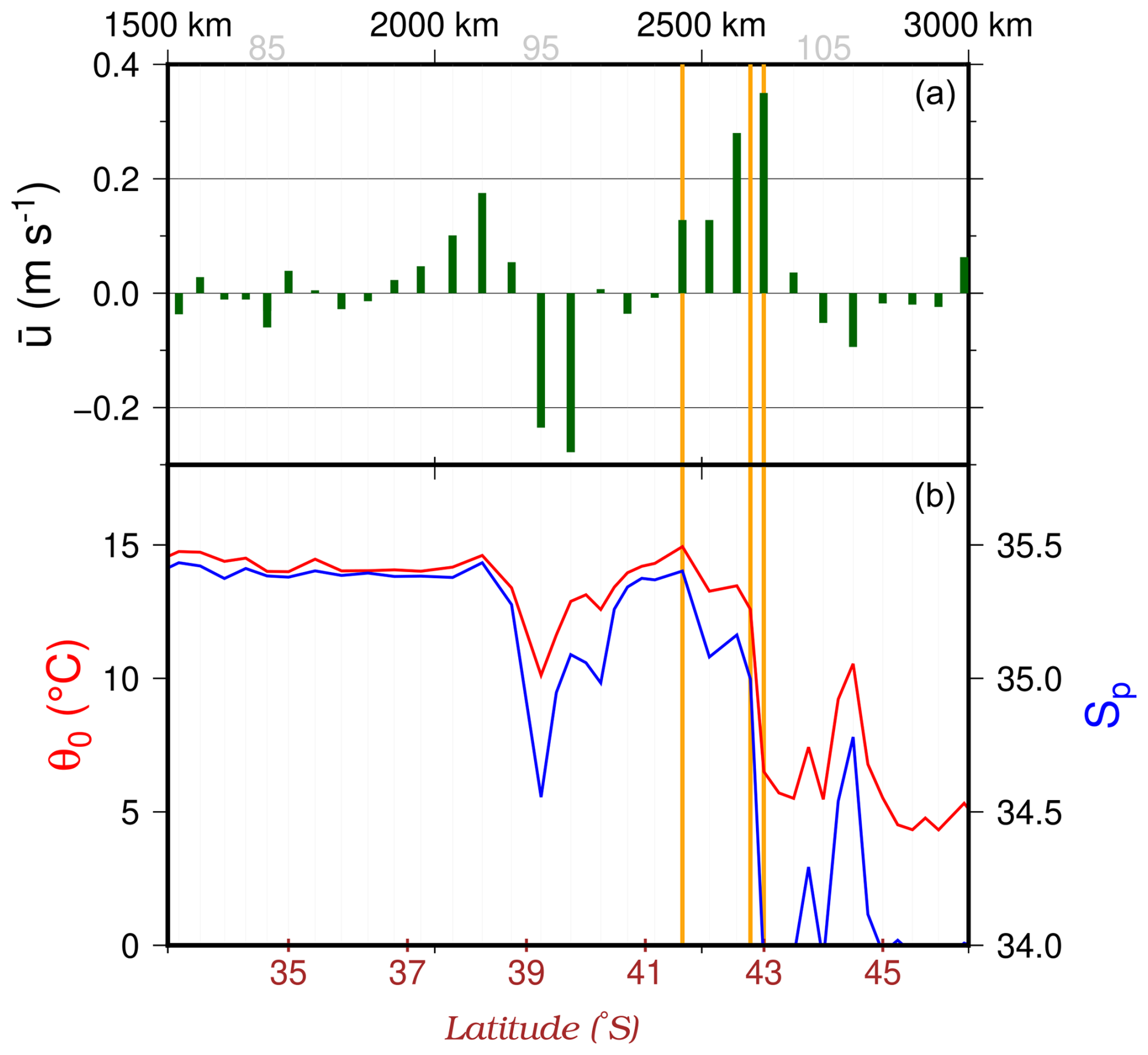
Figure 3 Zonal velocity averaged over the water column ($\stackrel{\mathrm{‾}}{u}$, a) and potential temperature (θ₀, red) and practical salinity (S_p, blue) at 200 dbar depth. The zonal velocity is positive eastward. The traditional potential temperature and practical salinity scale are used in this figure to facilitate comparison with previous publications. The horizontal axes are distance X (upper axis) like in Fig. 4 and latitude (lower axis). The vertical grid lines indicate the location of the CTD stations (does not include XCTD stations) with station numbers shown on the upper horizontal axis in grey. The vertical orange lines show estimated approximate positions of the Agulhas Return Current front, Subtropical Front, and Subantarctic Front (from north to south).

These front definitions as they apply to the I07S section are summarised in Table 2, which also lists the major southerly fronts defined by Orsi et al. (1995). The Southern ACC Front is found at around 62.5° S. At around 64.8° S, the Southern Boundary of the ACC passes over the continental slope at about 3000 dbar depth. These locations are consistent with those reported in Williams et al. (2010), who indicated that the Weddell Gyre is limited to the area west of Cape Ann.

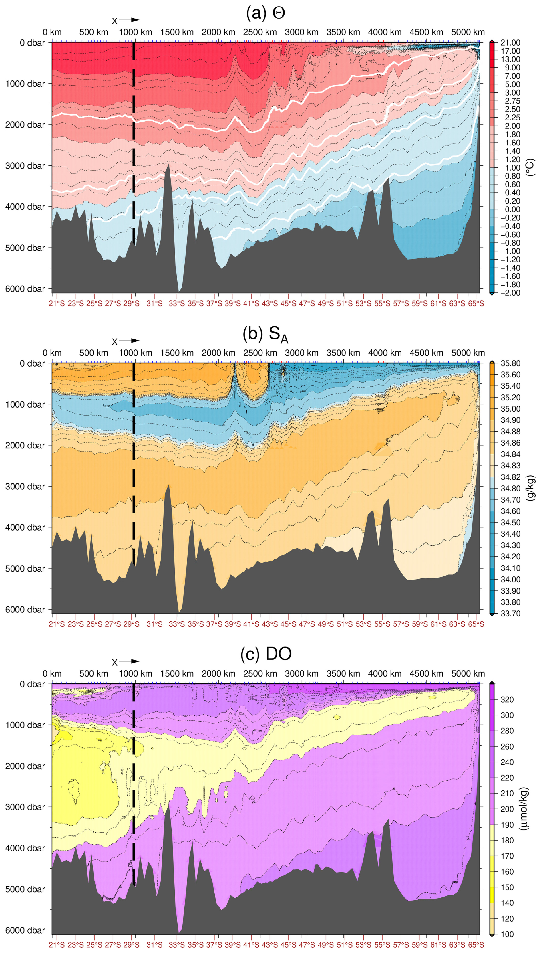
Figure 4 (a) Conservative Temperature Θ (°C), (b) Absolute Salinity S_A (g kg⁻¹), and (c) dissolved oxygen (µmol kg⁻¹) observed along the I07 section. The section north of 29.5° S (vertical dashed line) was occupied from April to May 2018 during cruise 33RO20180423, and the section south of 29.5° S was occupied from December 2019 to January 2020 during cruise 49NZ20191229. The upper horizontal axis shows the distance (X) from Station 26 of cruise 33RO20180423 at 54.517° E, 20.502° S. The corresponding latitudes are denoted in the lower axis with brown ticks and labels. The blue and red ticks on the upper horizontal axis show the position of CTD and XCTD casts, respectively. The vertical axis shows pressure. In (a), the white contours indicate neutral densities of γⁿ=27.9, 28.11, 28.18, and 28.27.

Table 1 Cruises. The cruises for sections I07S, I07N, I06S, I08S, and I05 are under the Global Ship-based Hydrographic Investigations Program (or its predecessor World Ocean Circulation Experiment). KH19 and KH20 are cruises on board R/V Hakuho (Ohashi et al., 2022). Others are cruises on board M/V Marion Dufresne (e.g. Park et al., 1991).

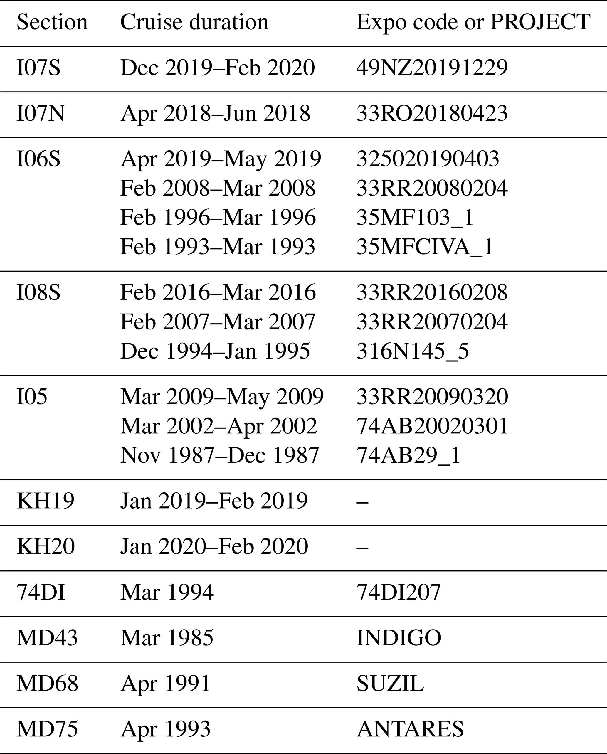
Table 2 Major fronts at 55° E. The traditional potential temperature (θ₀ in °C) and practical salinity (S_p, unitless in practical salinity scale) are used in this table to facilitate comparison with previous publications.

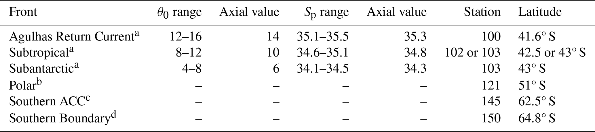
^a As defined by Park et al. (1991) using temperature and salinity at 200 dbar depth. ^b Northern limit of subsurface potential temperature minimum of θ₀=2 °C. ^c Potential temperature maximum θ₀>1.8 °C (Orsi et al., 1995). ^d Potential temperature maximum θ₀>1.5 °C (Orsi et al., 1995).

Hydrographic sections of temperature, salinity, and dissolved oxygen are shown in Fig. 4. The station interval of 30 nautical miles (15 nautical miles with XCTD) was found to be insufficient to separate the Subtropical and Subantarctic fronts. The low-salinity and low-temperature anomaly centred at 39° S (about X=2200 km) is a cyclonic (negative sea surface height anomaly) eddy, not a front. As seen in Fig. 5, our observation track passed very close to the eddy's centre, and the upward heave of isotherms and isohalines are striking. The ACC fronts are located around 41 to 43° S (X=2400 to 2600 km) (Fig. 5). The three northern fronts are accompanied by a strong eastward jet with a vertically averaged velocity >0.1 m s⁻¹, but the jet along the Polar Front is weaker at <0.03 m s⁻¹.

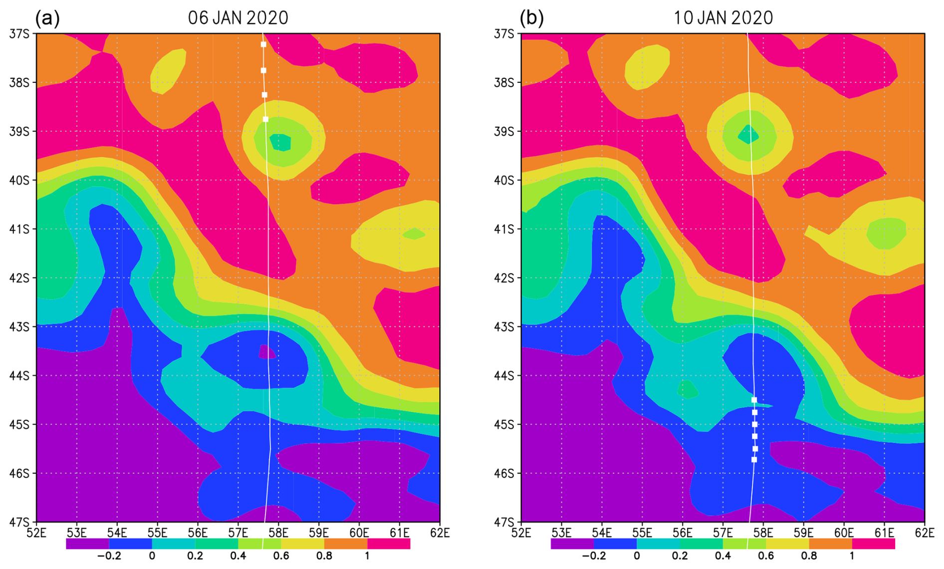
Figure 5 Two snapshots of the absolute dynamic topography: 6 January 2020 UTC (a) and 10 January 2020 UTC (b). The thin white line shows the cruise track, and the white squares show the CTD and XCTD stations occupied on each day.

A comparison of two snapshots obtained 4 d apart (Fig. 5) demonstrates that some eddies near the front (e.g. around 57.5° E, 43.5° S) were advected eastward, whereas others (e.g. 58° E, 39° S) moved westward, in agreement with the description by Park and Gambéroni (1997) that “even a section made in a few days across the frontal zone might not be considered as synoptic”.

The slopes of the isohaline and isotherms at the fronts are steep: S_A=34.82 g kg⁻¹ isohaline is at 560 dbar at X=2591.2 km and it crops out north of the next station at X=2616.4 km, whereas the Θ=9 °C isotherm jumps from 555 to 45 dbar between these stations. Both have a slope of $\mathrm{2}\times {\mathrm{10}}^{-\mathrm{2}}$. Because the meridional gradients of temperature and salinity are density-compensating, the slope of the corresponding isopycnal is smaller (506 to 271 dbar or $\mathrm{0.2}\times {\mathrm{10}}^{-\mathrm{2}}$).

The steep salinity front can be explained by surface forcing. The meridional gradient of surface salinity in the climatological data set (Mishonov et al., 2024) across these fronts (Fig. 6) is the strongest in the Southern Hemisphere. In such climatological data, the stationarity of the fronts also likely contributes to its large gradient. Strong evaporation in the midlatitude Indian Ocean results in a salty surface mixed layer. The salty surface water mass is advected by the Agulhas Current and returns in the Agulhas Return Current to the north of the fresh ACC, which amplifies the meridional haline gradient imprinted by precipitation minus evaporation.

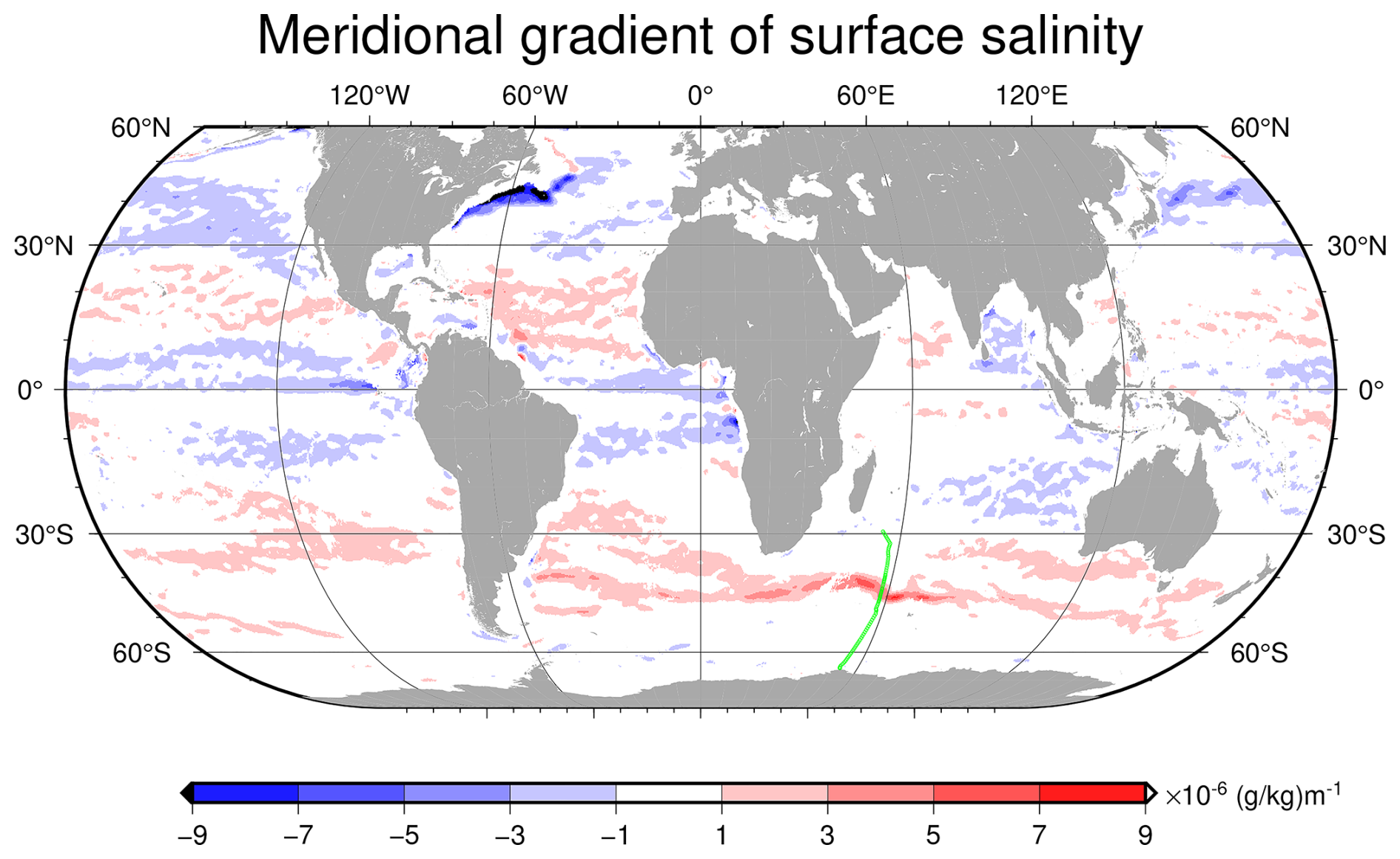
Figure 6 Meridional gradient of surface salinity from the World Ocean Atlas 2023 (Mishonov et al., 2024). The meridional gradient was calculated from the gridded salinity product on a $\mathrm{1}/\mathrm{4}$° grid. Large cross-shore gradients in coastal regions are avoided by restricting the plot to ocean depths >3000 m. The Arctic Ocean is also excluded. Green dots indicate the I07S stations.

Using data from a limited number of stations, Park et al. (1993) mapped dissolved oxygen at 3000 dbar depth (their Fig. 11) and found a frontal structure between 57° E, 32° S and 75° E, 43° S, separating low-oxygen North Indian Deep Water (NIDW) to the northeast from oxygen-rich Lower Circumpolar Deep Water (LCDW) to the southwest. Across the front, strong isopycnal mixing of NIDW and LCDW was inferred from the water properties. Our section (Fig. 4c) crosses the front at around 28° S (which was observed as part of I07N), showing the corresponding mesoscale structures north of 33° S at around 3000 dbar depth. The horizontal currents measured by LADCP appeared turbulent (not shown). This feature supports the inference by Park et al. (1993) that isopycnal mixing is strong across the front.

4 Deep circulation in the Enderby Basin

A snapshot of the horizontal circulation in the deep Enderby Basin is examined by plotting the LADCP data (Fig. 7). As suggested by the mean velocities, which are well within the variance ellipses, there is no obvious large-scale background flow. As the mesoscale wiggles of the sea surface height contours suggest, the field is characterised by numerous eddies, and our snapshot observation could not capture any mean transport. The eddies imply that the circulation in the deep Enderby Basin is diffusive in nature. It is possible to estimate vertical diffusivity from LADCP and CTD data by using a fine-scale internal wave parameterisation as is discussed in detail by Sasaki et al. (2024). We found that vertical diffusivity in the deep Enderby Basin is moderately strong (10⁻⁵ to 10⁻⁴ m² s⁻¹) and is enhanced towards the bottom. Using this vertical diffusivity, we attempted to estimate the horizontal diffusivity from the spatial distribution of transient tracers.

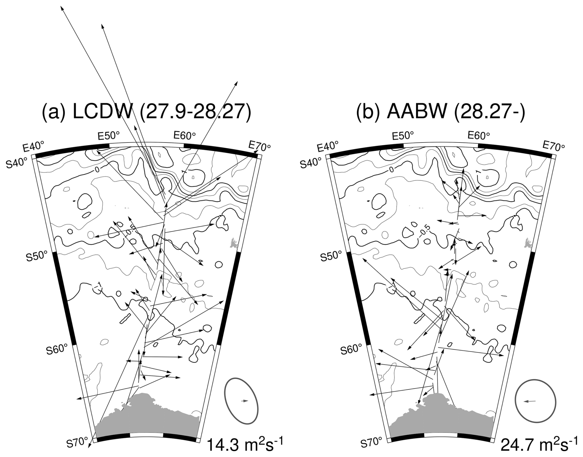
Figure 7 Instantaneous velocity observed by LADCP. (a) Horizontal velocity averaged within the LCDW layer (27.9 $<{\mathit{\gamma }}^n<$ 28.27) and (b) within the AABW layer (28.27 <γⁿ). The contours with intervals of 0.25 m (thin) and 0.5 m (thick, labelled) show the absolute sea surface height (SSH) field averaged over the cruise period (31 December 2019 to 22 January 2020). The SSH data are from satellite altimetry. The variance (ellipses) and mean (vectors) of the horizontal velocity in the Enderby Basin (defined here as south of 56° S) are shown at the bottom right corner of each panel. The vectors also give the scale.

4.1 Isopycnal diffusivity estimated from transient tracer distributions

Four kinds of transient tracers were measured along I07S. Here, we used CFC12 and SF₆ because CFC12 has had the highest atmospheric concentration since the 1970s and because the time evolution of SF₆ is quite different from that of CFC12.

As mentioned above, no obvious background flow was observed. Without any advecting mean flow, the concentration of a tracer in a meridional section $c(y,z,t)$ is governed by

$$\begin{array}{}\text{(1)}& {\displaystyle \frac{\partial c}{\partial t}}=K{\displaystyle \frac{{\partial }^{\mathrm{2}}c}{\partial y^{\mathrm{2}}}}+D{\displaystyle \frac{{\partial }^{\mathrm{2}}c}{\partial z^{\mathrm{2}}}},\end{array}$$

where t is time; the direction of y and z are northward along the isopycnal surfaces and across the isopycnal surfaces (positive towards the lighter density), respectively (McDougall, 1984); K is isopycnal diffusivity; and D is diapycnal diffusivity. Spatial and temporal variations of K and D are neglected. If we scale time by T, horizontal distance by $\sqrt{KT}$, and vertical distance by $\sqrt{DT}$, the equation becomes simply

$$\begin{array}{}\text{(2)}& {\displaystyle \frac{\partial c}{\partial t}}={\displaystyle \frac{{\partial }^{\mathrm{2}}c}{\partial y^{\mathrm{2}}}}+{\displaystyle \frac{{\partial }^{\mathrm{2}}c}{\partial z^{\mathrm{2}}}}.\end{array}$$

Profiles of the tracers (Fig. 8b and e) clearly show that dense shelf water with high tracer concentrations flows along the continental slope of Antarctica. We approximate this slope as a vertical wall and model this situation by considering two time-dependent tracer sources: one is a point source at the bottom of the slope and the other is a line source placed along the southern vertical wall. It might be that the possible deep eastern boundary current along the western flank of the Kerguelen Plateau injects additional tracers, but this effect cannot be included in our meridional two-dimensional model, and we regard this effect as part of the uncertainty. The point source represents young dense water masses carried westward by the Antarctic Slope Current, possibly including some contribution from the Australia–Antarctic Basin through the Princess Elizabeth Trough, whereas the line source is the newly ventilated water flowing along the continental slope. In neutral density coordinates (Fig. 8a and c), the point source is at $(y,z)=(\mathrm{0},\mathrm{0})$ and the line source is at y=0. We designate tracer distribution originating from the point source as c₀ and that originating from the line source as c₁ and seek a solution as their superposition:

$$\begin{array}{}\text{(3)}& c(y,z,t)={\mathit{\alpha }}_{\mathrm{0}}{c}_{\mathrm{0}}(r,t)+{\mathit{\alpha }}_{\mathrm{1}}{c}_{\mathrm{1}}(y,t),\end{array}$$

where α₀ and α₁ are constants to be determined. The solution c₀(r,t) is governed by Eq. (2) and is given in cylindrical coordinates with $r=\sqrt{y^{\mathrm{2}}+z^{\mathrm{2}}}$:

$$\begin{array}{}\text{(4)}& {\displaystyle \frac{\partial c_{\mathrm{0}}}{\partial t}}={\displaystyle \frac{\mathrm{1}}{r}}{\displaystyle \frac{\partial c_{\mathrm{0}}}{\partial r}}+{\displaystyle \frac{{\partial }^{\mathrm{2}}{c}_{\mathrm{0}}}{\partial r^{\mathrm{2}}}},\end{array}$$

with the boundary conditions

$$\begin{array}{}\text{(5)}& \begin{array}{rl}{c}_{\mathrm{0}}(r=\mathrm{0},t)& =s_{\mathrm{0}}(t-{\mathit{\delta }}_{\mathrm{0}})\\ {\displaystyle \frac{\partial c_{\mathrm{0}}(y=\mathrm{0},t)}{\partial z}}& ={\displaystyle \frac{\partial c_{\mathrm{0}}(z=\mathrm{0},t)}{\partial y}}=\mathrm{0},\end{array}\end{array}$$

where the time offset δ₀ is the advection time from the surface mixed layer to the I07S section, and s₀ is the source of the tracer as a function of time. The solution c₁(y,t) is governed by

$$\begin{array}{}\text{(6)}& {\displaystyle \frac{\partial c_{\mathrm{1}}}{\partial t}}={\displaystyle \frac{{\partial }^{\mathrm{2}}{c}_{\mathrm{1}}}{\partial y^{\mathrm{2}}}},\end{array}$$

with the boundary conditions

$$\begin{array}{}\text{(7)}& \begin{array}{rl}{c}_{\mathrm{1}}(y=\mathrm{0},t)& =s_{\mathrm{1}}(t-{\mathit{\delta }}_{\mathrm{1}})\\ {\displaystyle \frac{\partial c_{\mathrm{1}}(y=\mathrm{0},t)}{\partial z}}& =\mathrm{0},\end{array}\end{array}$$

where δ₁ is, again, the advection time, which can be different from δ₀, and s₁ is the source function. The sum α₀c₀+α₁c₁ only approximately satisfies the boundary condition at the southern boundary y=0, which is a limitation of this model. The governing Eqs. (4) and (6) were numerically solved with realistic source functions s₀(t) and s₁(t). We take the unit time as T=1 year. Calculations were carried out for the years 1950 to 2020 with a non-dimensional grid spacing of 0.1 for $\mathrm{0}<r<\mathrm{50}$ and $\mathrm{0}<y<\mathrm{50}$. The source functions reflect the atmospheric concentration of the tracers, which is converted to the concentration within the mixed layer by laboratory-determined solubility (Warner and Weiss, 1985; Bullister et al., 2002) at an assumed seawater temperature of 0 °C, salinity of 34.5 practical salinity units, and a constant saturation rate. A typical observed saturation rate is 70 % (Schlosser et al., 1991; Ohashi et al., 2022), but the tracers in the dense shelf water are diluted when they form the source water at depth. We tested saturation rates between 35 % and 70 % and found an overall error similar to that for saturation rates between 50 % and 70 % but greater for smaller saturation rates. We therefore use a saturation rate of 50 % here. The atmospheric concentration before 2015 is taken from Bullister and Warner (2017) and that after 2015 from the NOAA Global Monitoring Laboratory, following Ohashi et al. (2022).

A non-linear least squares fit of Eq. (3) (Levenberg–Marquardt method; Madsen et al., 2004) was used to find the values of α₀, α₁, δ₀, δ₁, and K that minimise the difference between the predicted and observed concentration of CFC12 and SF₆. In the calculation of this difference, the source area was excluded by limiting the comparison to observed concentrations of <0.4 pmol kg⁻¹ for CFC12 and <0.21 fmol kg⁻¹ for SF₆; thus we fit Eq. (3) to 125 and 118 bottle measurements for CFC12 and SF₆, respectively. To estimate the isopycnal diffusivity K, we used the fixed diapycnal diffusivity of $D=\mathrm{4.7}\times {\mathrm{10}}^{-\mathrm{5}}$ m² s⁻¹, which is the arithmetic mean of the diapycnal diffusivity below 2000 dbar between 56 and 63.5° S estimated by fine-scale parameterisation (Polzin et al., 2014) of the observed stratification and horizontal velocity field (Katsumata et al., 2021). The observed diapycnal diffusivity showed some spatial variability (Fig. 8c), and the diffusivity is high where the near-bottom CFC12 concentration is high (Y=400 to 700 km in Fig. 8a and b). We neglect this spatial variability. Next, we prescribe a set of initial values, namely at α₀=0.1, α₁=0.1, and K=500 m² s⁻¹, for fitting by the Levenberg–Marquardt method. The advection times δ₁ and δ₀ are each set at 0, 1, … 19 years, giving 400 combinations of δ₁ and δ₀ for the non-linear least squares calculation; thus we obtain 400 sets of α₁, α₂, and K. We tried several different sets of initial values (for example K=100 m² s⁻¹), but they converged to the same solution.

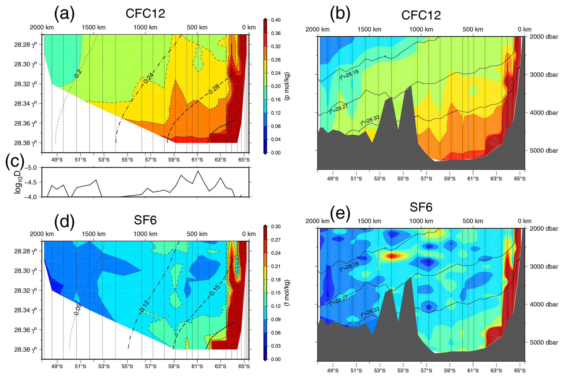
Figure 8 Concentrations of transient tracers (a, b) CFC12 and (d, e) SF₆. The horizontal axes show latitude (bottom) and distance (Y, top) from the southernmost station, and the vertical axis shows density in (a) and (d) and pressure in (b) and (e). The colours in (a) and (b) show the concentration of CFC12 (in pmol kg⁻¹), whereas those in (d) and (e) show the concentration of SF₆ (in fmol kg⁻¹). The contours in (a) and (d) show the concentrations predicted by the simple diffusion model (3) with α₀=0.12, δ₀=10, α₁=0.14, and δ₁=16. The same types of contour lines are used for observed and predicted quantities. The contours in (b) and (e) show the isopycnals γⁿ=28.18, 28.27, and 28.33. The observed concentrations in the pressure vertical coordinate in (b) and (e) are converted to the density vertical coordinate in (a) and (d). Panel (c) shows diapycnal diffusivity D averaged below 2000 dbar.

The error did not show an obvious sharp global minimum. The global minimum error (sum of squares) was 0.117 for the 400 sets of trials and the error histogram (not shown) is a decreasing function of the error with a change in the decreasing slope with an error equal to 0.25. We thus selected the 160 parameter sets with an error <0.25 as good estimates. The averages and standard deviations of the good estimates are ${\mathit{\delta }}_{\mathrm{0}}=\mathrm{10}\pm \mathrm{6}$ years, ${\mathit{\delta }}_{\mathrm{1}}=\mathrm{16}\pm \mathrm{3}$ years, ${\mathit{\alpha }}_{\mathrm{0}}=\mathrm{0.12}\pm \mathrm{0.04}$, ${\mathit{\alpha }}_{\mathrm{1}}=\mathrm{0.14}\pm \mathrm{0.01}$, and $K=\mathrm{72}\pm \mathrm{16}$ m² s⁻¹. We note that this uncertainty does not include the contribution due to the simplification introduced in our crude model such as spatial variability of the diapycnal diffusivity D and temporal change of source saturation rate. These mean values are used in Fig. 8. The “age” of the source water (δ₀ and δ₁) appears to be overestimated compared with ages obtained by other methods (e.g. Ohashi et al., 2022); possible reasons include the saturation uncertainty or a limitation due to the idealised source function.

The estimated isopycnal diffusivity of $K=\mathrm{72}\pm \mathrm{16}$ m² s⁻¹ is not much different from past estimates in deep seas. For example, the isopycnal diffusivity at 4000 dbar in the Atlantic Ocean has been estimated by an artificial tracer release experiment to be about 100 m² s⁻¹ (Ledwell, 2024). Phillips and Rintoul (2000) have estimated horizontal temperature diffusivity near the Subantarctic Front, south of Australia, to be 100 to 200 m² s⁻¹ at 2240 and 3320 dbar. Our value is also similar to the isopycnal diffusivity on the continental rise in the Australia–Antarctic Basin (Katsumata and Yamazaki, 2023) and a deep diffusivity of 30 to 70 m² s⁻¹ estimated by a plume model of AABW based on the observation of transient tracers in the Weddell Sea (Haine et al., 1998). The diffusive nature of the interior circulation also agrees with the CFC distribution in Fine et al. (2008, their Fig. 5), with sparse contours in the interior of the Enderby Basin compared to packed contours found in near-boundary regions. The tracer distribution thus suggests that circulation in the deep Enderby Basin is mostly dominated by the westward transport near the Antarctic slope and isopycnal interior diffusion. The diffusivity value is typical of that for deep basins, where values are weaker than those observed in the upper water column (500 to 1000 m² s⁻¹; e.g. Tulloch et al., 2014).

4.2 AABW composition

The Enderby Basin collects AABW from four major sources: Weddell Sea Deep Water (WSDW), Cape Darnley Bottom Water (CDBW), Adélie Land Bottom Water (ALBW), and Ross Sea Bottom Water (RSBW). WSDW arrives at the I07S section from the west, while ALBW and RSBW flow through the Princess Elizabeth Trough further to the east (Heywood et al., 1999).

Previous occupations of GO-SHIP sections I06S at 30° E and I08S at 85° E provide information on how WSDW and ALBW–RSBW each contribute to AABW at I07S (Fig.  9).

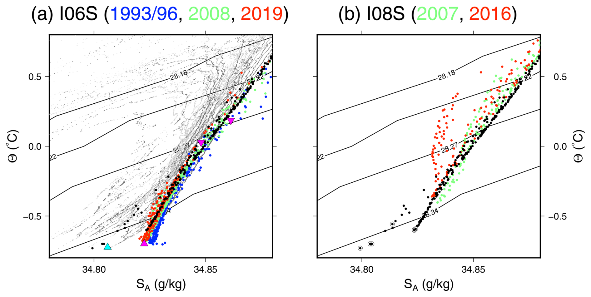
Figure 9 Temperature–salinity diagrams of the bottom waters at 30° E (I06S, a) and at 82° E (I08S, b) based on data from different occupation years (indicated by the colours of the circles). Black points show the data of I07S observed in 2019/20, and the dark- and light-grey points show data of R/V Hakuho (KH) cruises in 2019 and 2020, respectively (see Fig. 1). For I06S, only bottle data collected at depths with density γⁿ>28.0 are shown. For I08S, only bottle data from south of 60° S at depths with density γⁿ>28.0 and deeper than 1000 dbar are shown. For I07S, only bottle data at depths with density γⁿ>28.0 and deeper than 3000 dbar are shown. In (b) data points for the deepest bottles (i.e. 10 m above the seafloor) and south of 60° S along the I07S section (black points) are circled. The source waters used in the mixing analysis are indicated by triangles: LCDW by inverted magenta triangles (S_A=34.86 g kg⁻¹, $\mathrm{\Theta }={\mathrm{0.19}}^{\circ }$C; S_A=34.85 g kg⁻¹, Θ=0.03 °C), WSDW by the magenta triangle (S_A=34.82 g kg⁻¹, $\mathrm{\Theta }=-\mathrm{0.70}$ °C), and CDBW by the cyan triangle (S_A=34.81 g kg⁻¹, $\mathrm{\Theta }=-\mathrm{0.72}$ °C). Density contours γⁿ=28.18, 28.22, 28.27, and 27.34 are shown.

On the temperature–salinity diagram, points for upper AABW ($\mathrm{28.18}<{\mathit{\gamma }}^n<\mathrm{28.33}$) on I08S are scattered (Fig. 9) because these densities on the shelf are subject to direct atmospheric forcing. The deep water masses are, however, similar to I07S within the AABW range ($\mathrm{28.27}<{\mathit{\gamma }}^n<\mathrm{28.34}$). Menezes et al. (2017) have reported freshening of bottom water in the Princess Elizabeth Trough. On I06S, points for the lighter water masses γⁿ<28.22 are similarly scattered. On I06S below γⁿ=28.22, persistent freshening from 1993 to 2008 is discernible, and the water on I07S appears to be in between the 2008 and 2019 water masses observed along I06S. Haine et al. (1998), using CFCs, estimated the mean transient time from the Greenwich meridian (0° E) to the Crozet–Kerguelen gap (55° E) along the southern flank of the Southwest Indian Ridge as 12 to 20 years (their Fig. 5) depending on the diffusion assumptions adopted. The transient time between 30 and 55° E is likely half that, i.e. 6 to 10 years. We therefore use the 2008 observations on I06S as the source water in our mixing model.

We note that the bottom water on I08S was not dense enough to explain the near-bottom water (>28.34) observed at I07S. We thus conclude that the densest class of AABW (γ>28.34) observed on I07S is a mixture of WSDW and CDBW.

Orsi et al. (1999) called the water mass with $\mathrm{28.18}<{\mathit{\gamma }}^n<\mathrm{28.27}$ “ACC Bottom Water” (ACCbw) because it is well mixed and shows little zonal variability compared to the water masses above or below. The focus in this section is thus on water masses deeper than γⁿ=28.27, which fill the Enderby Basin and, south of 39° S, the Crozet Basin (Fig. 4a). Here we estimate the composition of AABW (γⁿ>28.27) in the Enderby Basin using a method following that used in Johnson (2008), i.e. least squares fitting with a non-negative constraint in which temperature, salinity, PO${}^{*}=\mathrm{170}[$PO₄]+[O₂], NO${}^{*}=\mathrm{10.625}[$NO₃]+[O₂], and SO${}^{*}=\mathrm{1.66}[$SO₄]+[O₂] are conserved. The method yields six equations (one being mass conservation). We do not expect potential vorticity to be conserved because the flow is subject to bottom friction. The weights for the conservation equations are taken from Johnson (2008): 1, 0.25, 1, 0.5, 0.5, and 0.25 for mass, temperature, salinity, PO^*, NO^*, and SO^*, respectively. As reflected in their relatively small weights, the pseudo-tracers, PO^*, NO^*, and SO^*, do not provide strong constraints as manifested by the almost linear distribution of the data points when they are plotted against temperature (Appendix, Fig. B1).

The number of the unknowns (source water masses) is four: two are CDBW and WSDW, and LCDW, which overlies these AABW, is expressed by the linear combination of two extremes (warm–salty and cold–fresh), which we call LCDW1 and LCDW2. It is possible that the bottom waters from the Ross Sea (RSBW) and Adélie Land (ALBW) cross the I07S section after flowing through the Princess Elizabeth Trough, but some previous studies have suggested otherwise.

A numerical simulation by Kusahara et al. (2017) indicates that bottom waters that have passed through Princess Elizabeth Trough form a deep eastern boundary current flowing along the west coast of the Kerguelen Plateau, i.e. eastward of 60° E (their Fig. 8a and b), and do not spread into the Enderby Basin. Aoki et al. (2020a) also reported that south of 62° S near the bottom (within 300 dbar of the seabed), influences by RSBW and ALBW were discernable only at 70° E and not at 60° E. We therefore neglect the contributions from ALBW and RSBW to the interior of Enderby Basin. We expect that LCDW originates mostly from the upstream ACC. As seen in Fig. 9, LCDW in the interior Enderby Basin is not a homogeneous water mass but shows a range of temperatures and salinities. We thus chose two end points and express the range as the mixing (linear combination) of these two. One end point is Station 31 (42.5° E, 30° S) at a depth of 4670 dbar (γⁿ=28.265), and the other is Station 50 (52.0° E, 30° S) at a depth of 3210 dbar (γⁿ=28.279). For WSDW, we use data from the bottom (5245 dbar) bottle at Station 71 (γⁿ=28.4) from the 2008 I06S occupation. CDBW is represented by the C03 station of the KH19 cruise (61.81° E, 63.1° S) at a sampling depth of 4542 dbar (γⁿ=28.394) because the water properties there (S_A=34.81 g kg⁻¹, $\mathrm{\Theta }=-\mathrm{0.72}$ °C) are closest to the average value for CDBW measured by a year-long mooring (S_A=34.807 g kg⁻¹, $\mathrm{\Theta }=-\mathrm{0.777}$ °C when converted to the Thermodynamic Equation of SeaWater 2010 (TEOS-10) value) near Cape Darnley (Ohshima et al., 2013).

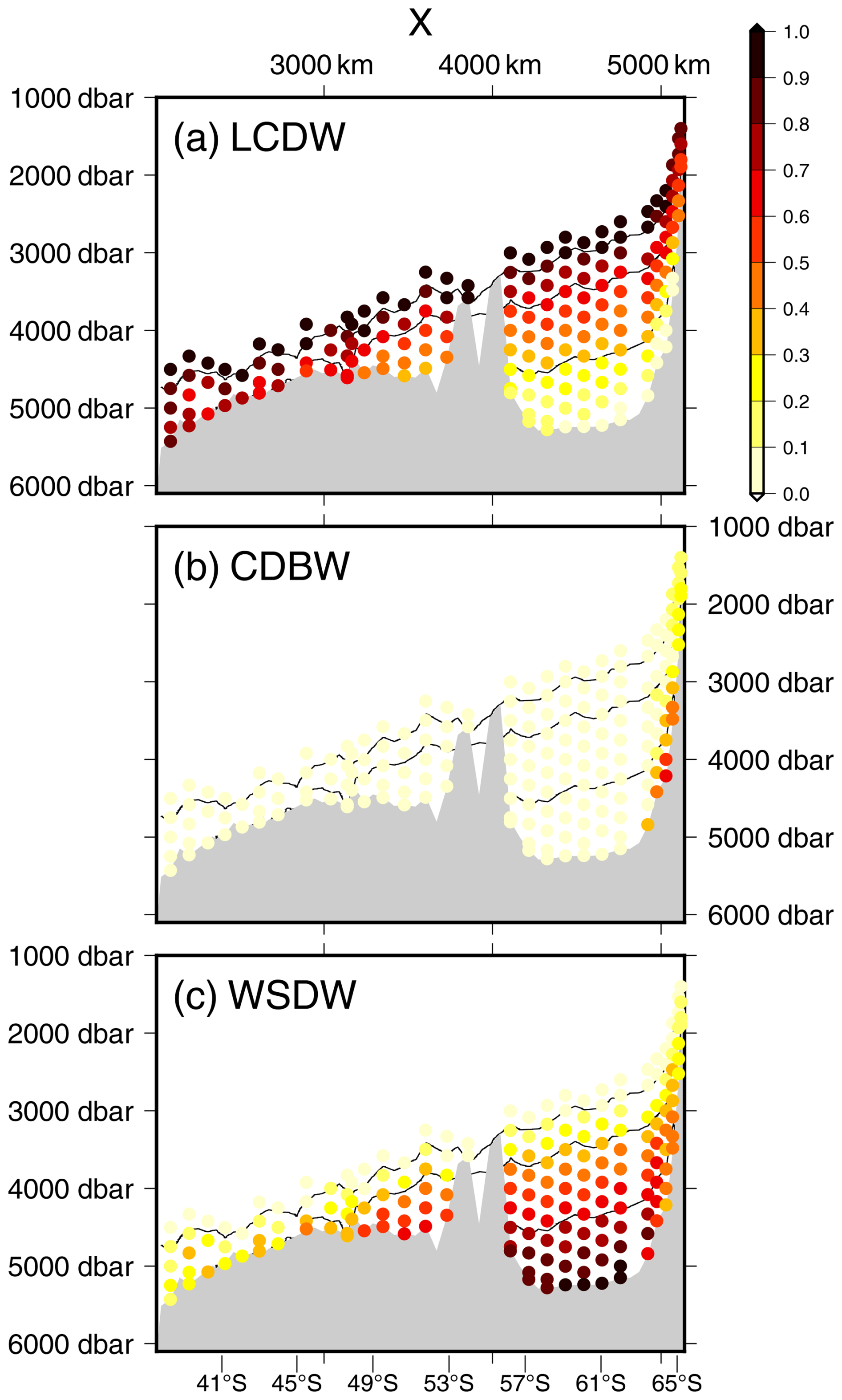
Figure 10 Mixing ratio of sources for Antarctic Bottom Water in the Enderby and Crozet basins along the I07S section. The upper horizontal axis shows distance X, and the bottom axis shows approximate latitude. The vertical axis shows pressure. The contours are isopycnals at γⁿ=28.27, 28.30, and 28.35.

The mixing ratios in Fig. 10 show some scatter, but the overall composition of AABW varies roughly with density. For γⁿ=28.27, CDBW =0 % to 20 %, WSDW =5 % to 35 %, and LCDW = LCDW1+LCDW2 =70 % to 95 %. The contribution changes approximately linearly towards γⁿ=28.35, where CDBW =0 % to 35 %, WSDW =35 % to 75 %, and LCDW =25 % to 45 %. As expected from the closeness of the I07S temperature and salinity to those of I06S (Fig. 9a), AABW in the Enderby Basin consists mostly of WSDW with a little contribution from CDBW. Near the shelf (X>5000 km, south of 63° S), near-bottom-water mass shows a considerable contribution from CDBW, as indicated by several isolated and relatively fresh points on the temperature–salinity diagram (Fig. 9).

We examined the sensitivity of the results to the choice of source water masses. For WSDW, Station 70 (30.0° E, 62.0° S; 5267 dbar), Station 69 (30.0° E, 61.5° S; 5294 dbar), Station 73 (30.0° E, 63.5° S; 5217 dbar), and Station 75 (30.0° E, 64.5° S; 5105 dbar) were substituted for the original source water at Station 69. Similarly for CDBW, C02 (59.45° E, 63.50° S; 4370 dbar), C04 (63.69° E, 64.10° S; 3922 dbar), C05 (65.20° E, 64.96° S; 3364 dbar), and C06 (66.25° E, 65.50° S; 3363 dbar) were each substituted. From these combination we obtained 25 pairs of calculations: the spreads of the results at Stations 134 (L=4215 km, 57.22° S), 142 (L=4650 km, 61.09° S), and 148 (L=4975 km, 63.97° S) are shown in Fig. 11. Because LCDW is represented by the linear combination of two extremes, the sensitivity to LCDW was not examined.

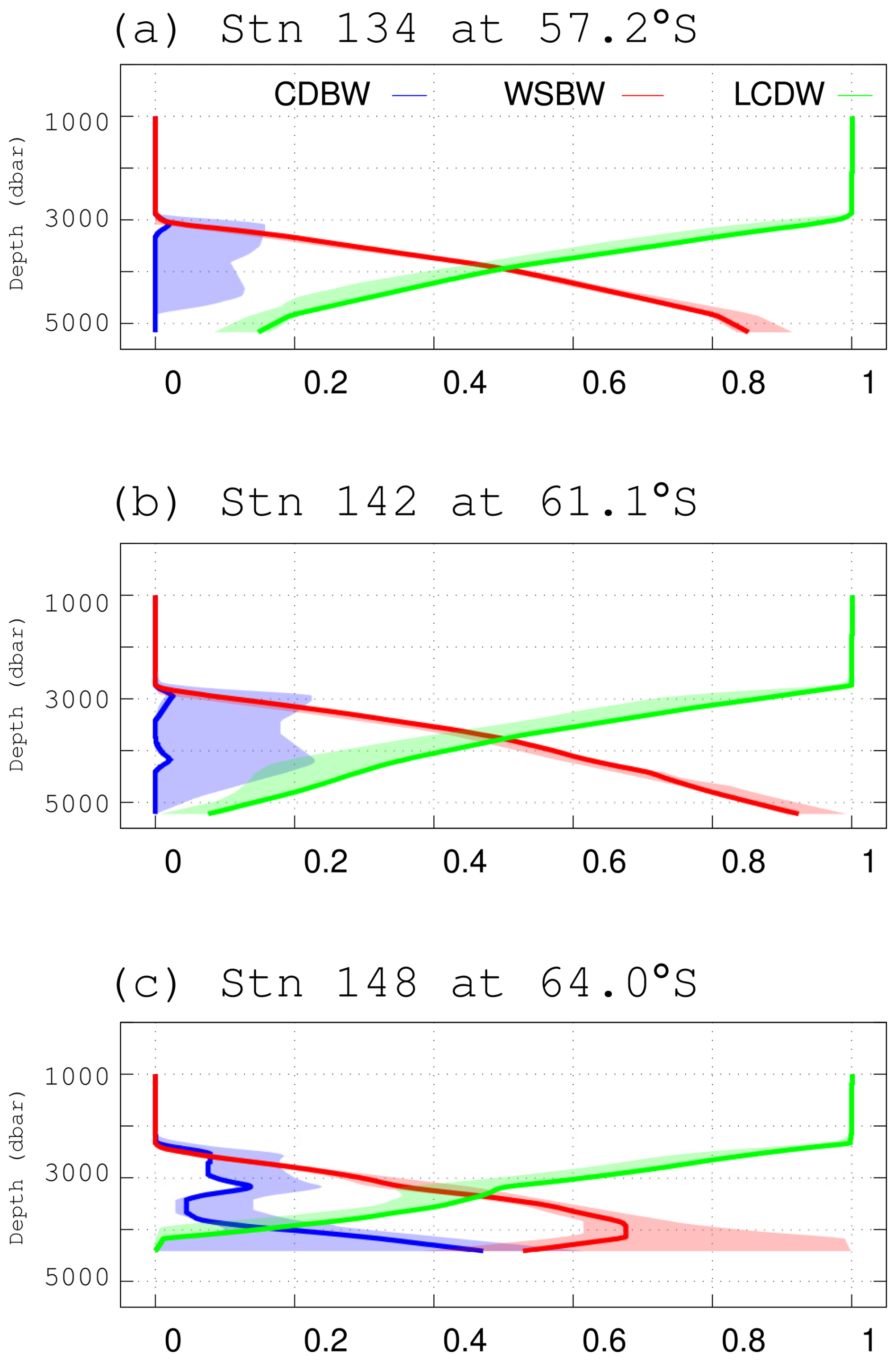
Figure 11 Vertical profiles of the estimated composition (horizontal axes) of AABW in the Enderby Basin. The contributions from Cape Darnley Bottom Water (CDBW), Weddell Sea Deep Water (WSDW), and Lower Circumpolar Deep Water (LCDW) are shown by blue, red, and green lines, respectively, and the accompanying shading shows the spread (minimum and maximum) of the estimates for 25 pairs obtained using different choices for CDBW and WSDW properties. The bottle data were vertically interpolated by the method of Reiniger and Ross (1968).

The estimates for CDBW and WSDW show an uncertainty of ±20 % or greater. In contrast, the estimates for LCDW show a smaller spread. The uncertainty does not change the qualitative conclusion that the contribution of WSDW to the AABW in the Enderby Basin is greater than that of CDBW.

5 Conclusions

In this paper, results from a 2019 cruise along 55° E south of 30° S are delineated with emphasis on deep to bottom circulations. At 55° E, the deep to bottom circulation is primarily diffusive with no obvious mean flow – thus transient tracers show equatorward spread in accordance with the large-scale meridional gradient. In this sense, the eastern boundary of the Weddell Gyre does not reach as far east as 55° E.

Because the 2019 cruise was the first occupation of the new GO-SHIP section I07S, only 11 previously occupied stations were revisited (Table A1 in Appendix). In the present comparison, the bottom salinity “rebound” in the Australia–Antarctic Basin, which was reported to be propagating westward (Aoki et al., 2020b), was not detected. The next GO-SHIP occupation of the I07S section will measure changes in the Enderby Basin not only in temperature and salinity but also in other parameters that were sampled during the 2019 cruises, including nutrients calibrated against certified reference materials and biological parameters such as microbial diversity and abundance.

Appendix A: Decadal changes in water mass properties

Table A1 Summary of water temperature changes ΔΘ (°C) and salinity changes ΔS_A (g kg⁻¹) on isopycnals from observations before the 2019/20 occupation. n/a – not applicable.

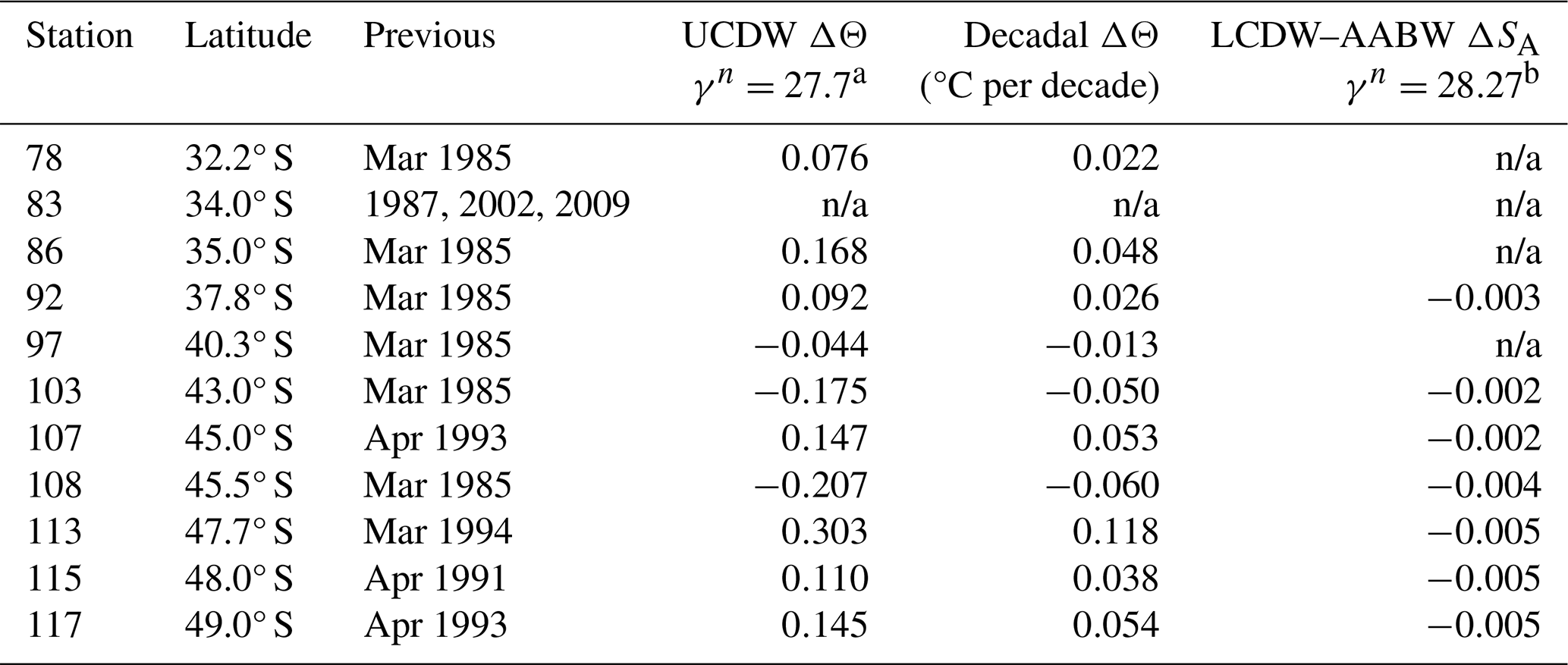
^a Upper Circumpolar Deep Water (UCDW) is represented at this density. Θ is Conservative Temperature. ^b Lower Circumpolar Deep Water (LCDW) and Antarctic Bottom Water (AABW) are represented at this density. S_A is Absolute Salinity.

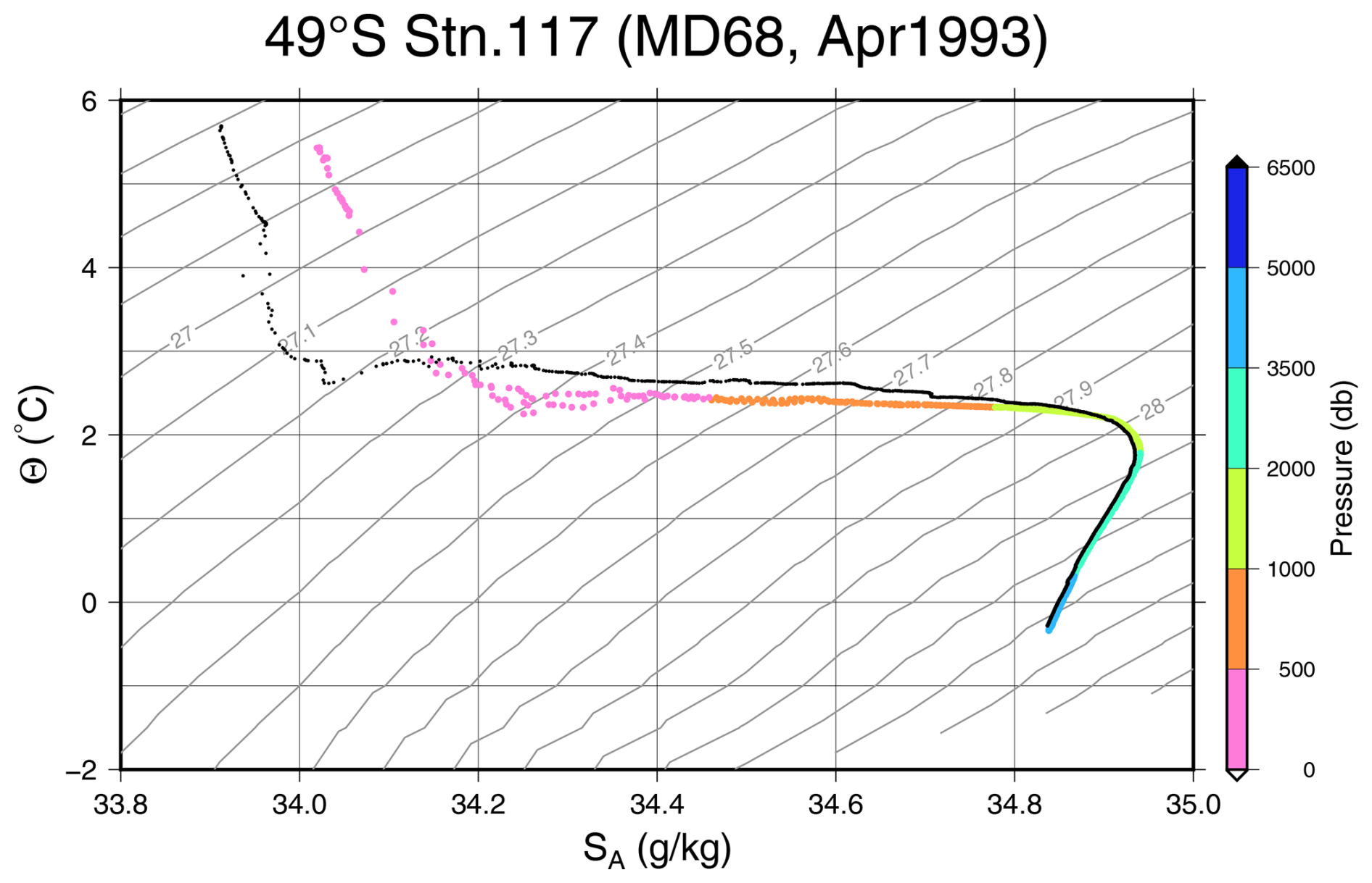
Figure A1 Water properties at Station 117, which was occupied during cruise MD68 by M/V Marion Dufresne in April 1993 (coloured points; the different colours indicate depth). Black points show the 2019/20 occupation results.

Eleven stations were reoccupations of previous stations (defined as stations within 20 km of our stations) at which high-precision hydrographic data had been obtained. The observed changes since the previous occupation are summarised in Table A1, and those at Station 117 and Station 83 are shown in Figs. A1 and A2, respectively.

It is known that the standard seawaters used for bottle salinity measurements have batch-to-batch offsets of the order of 10⁻³ in the practical salinity scale (Uchida, 2019). These offsets were corrected by using the coefficients by Uchida (2019), but the correction was not possible for M/V Marion Dufresne cruises because the batch numbers for these cruises are not known. The M/V Marion Dufresne cruises used in Table A1 were conducted in 1985, 1991, and 1993. During the late 1980s to the early 1990s, cruise reports for cruises conducted under World Ocean Circulation Experiment documented the use of standard seawater batches from P96 to P118. The offsets for these batches scatter between $-\mathrm{0.9}\times {\mathrm{10}}^{-\mathrm{3}}$ to $\mathrm{2.5}\times {\mathrm{10}}^{-\mathrm{3}}$. It is therefore likely that salinity from M/V Marion Dufresne cruises has offsets of $(-\mathrm{1}\sim \mathrm{3})\times {\mathrm{10}}^{-\mathrm{3}}$. In addition to the batch offset, the measurement accuracy for the M/V Marion Dufresne cruise was 0.003 practical salinity units (approximately 0.003 g kg⁻¹) (Park et al., 1993). The accuracy for GO-SHIP cruises is 0.002 g kg⁻¹ (Hood, 2010). The combined accuracy for the two cruises is therefore 0.004 g kg⁻¹. Adding this accuracy to the batch offset, we note that salinity differences between the I07S cruise and M/V Marion Dufresne cruises of less than 0.007 g kg⁻¹ are probably not significant. For 74DI207 at Station 113, the cruise documentation records the use of batches P120 and P123, but it was not clear which was used for station 12644 used for our comparison in Table A1. The comparison without the batch correction shows freshening of bottom water. We therefore assumed the use of P120 (batch offset $-\mathrm{0.9}\times {\mathrm{10}}^{-\mathrm{3}}$) rather than P123 ($\mathrm{0.7}\times {\mathrm{10}}^{-\mathrm{3}}$) to conservatively estimate the salinity change. The batch offsets have been applied for station 83.

In Table A1, the changes in temperature and salinity were compared on isopycnals γⁿ=27.7 and 28.27. Since previous and present data were at the same density,

$$\begin{array}{}\text{(A1)}& \mathrm{0}=\mathrm{\Delta }\mathit{\rho }(\mathrm{\Theta },S_{\mathrm{A}},p)=\mathit{\rho }(-\mathit{\alpha }\mathrm{\Delta }\mathrm{\Theta }+\mathit{\beta }\mathrm{\Delta }{S}_{\mathrm{A}}),\end{array}$$

where α is the thermal expansion coefficient, and β is the haline contraction coefficient. Once ΔΘ is known, it is possible to calculate ΔS_A, and vice versa. Typical values of $\mathit{\alpha }/\mathit{\beta }$ are 0.21±0.03 for $\mathrm{\Theta }=\mathrm{1}\pm \mathrm{1}$ °C, $S_{\mathrm{A}}=\mathrm{34.9}\pm \mathrm{0.1}$, and $p=\mathrm{3500}\pm \mathrm{500}$ dbar, giving approximately a 1-to-5 ratio of ΔS_A to ΔΘ. We therefore use temperature for Upper Circumpolar Deep Water (UCDW) and salinity for LCDW–AABW.

UCDW became warmer by 0.09 to 0.17 °C except at the stations between 40.3 and 45.5° S, where the UCDW water mass is subject to frontal movements and accompanying mesoscale mixing such that the changes are neither systematic nor robust (see also Fig. A1). As pointed out in Sect. 3, UCDW has a dissolved oxygen front at around 27° S, and UCDW warming observed at stations 86 and 92 might suggest warming of the UCDW north of the front (North Indian Deep Water). Aoki et al. (2005) reported warm and salty anomalies in UCDW, which they attributed to mixing surface waters that were warmer and fresher because of climate changes. The UCDW warming found here confirms that this warming trend continued after the 1990s.

Due to the unknown possible salinity offsets of standard seawater, we cannot confidently conclude freshening of LCDW and AABW except at station 113. At station 113, a freshening of 0.005 g kg⁻¹ after application of the offset might be significant; however this station is located over the sill separating the Enderby and Crozet basins, and interpretation is difficult in the absence of other reliable data nearby.

Bryden et al. (2003) described the water mass changes at the cross point of the GO-SHIP I05 section and the I07S section at 34° S, with a focus on the water mass changes in the thermocline (as defined by potential temperature θ_σ>6 °C) or the mode waters in the northern Crozet Basin. Bryden et al. (2003) reported a freshening of the thermocline water mass (between potential temperatures of 7 and 10 °C) from 1987 to 2002. This cooling and freshening was also reported by Aoki et al. (2005). These changes are attributable to surface warming in response to atmospheric warming.

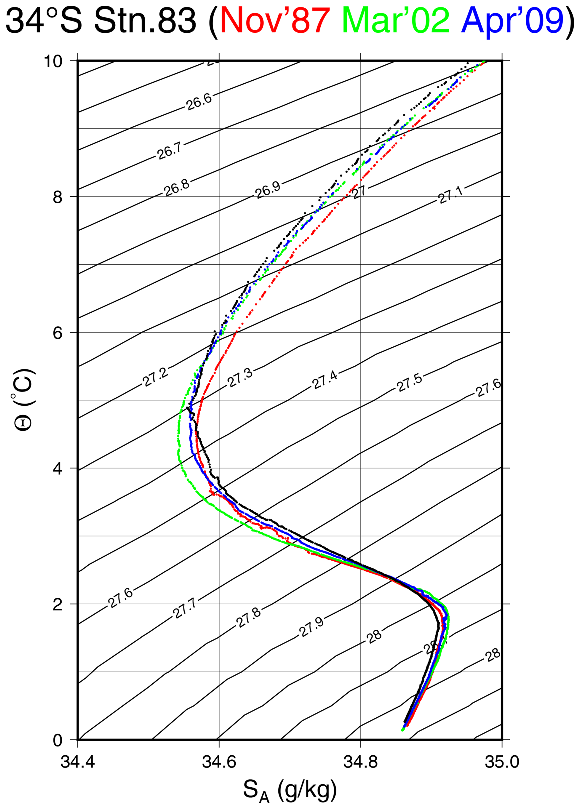
Figure A2 Water properties at Station 83, a part of the I05 section previously occupied in November 1987, March 2002, and April 2009. Data from these past occupations are shown with red, green, and blue dots, respectively, and our 2019 occupation data are shown with black dots.

The freshening of the thermocline water mass at Station 83 appears to have stopped from 2002 until 2009, after which it resumed (Fig. A2). This behaviour is different from that around the salinity minimum of Antarctic Intermediate Water (AAIW) where the freshening from 1987 to 2002 was as large as 0.02 g kg⁻¹ near the salinity minimum at γⁿ=27.4. After 2002 the change reversed, and the salinity minimum become saltier through 2009, continuing until 2019. The salinity maximum originating from North Atlantic Deep Water (NADW) at γⁿ=28.05 also shows the oscillation – saltier from 1987 to 2002 and then fresher through 2009 until 2019.

These property changes have often been attributed to meridional migration of the water masses (e.g. Gille, 2002). It is known in this region that the fronts, which are indicators of the meridional position of water masses, move southward on a decadal timescale (Sokolov and Rintoul, 2009; Kim and Orsi, 2014). Along the I07S section, sea surface height has increased by about 0.003 m yr⁻¹ north of 48° S (Fig. A3). Given the background gradient of approximately 2 m over 30° latitude, the fronts shifted southward by roughly $\mathrm{0.003}\times \mathrm{30}/(\mathrm{2}/\mathrm{30})=\mathrm{1.35}\mathit{°}$ of latitude over a period of 30 years. At the typical UCDW depth of 2000 dbar around 40° S, a close look at Fig. 4a shows that Θ does not show an obvious meridional gradient north of the Subtropical and Subantarctic fronts at 42° S. South of the fronts, the meridional gradient of Θ is about 0.1 °C per 1° latitude. A southward shift of the front can therefore explain the warming observed at Stations 113, 115, and 117. Salinity at the LCDW–AABW depth of 4000 dbar shows a persistent meridional gradient of about 0.0015 g kg⁻¹ per 1° latitude, but salinity is higher northward. A southward shift of the fronts cannot explain freshening observed at these depths. Thus a southward shift of the fronts across the I07S plausibly contributed to the UCDW warming observed south of 47° S, but other changes cannot be attributed to the meridional water mass movements.

Although the seven southernmost stations south of 64° S have been occupied three times (1994, 2012, and 2019), it is difficult to identify robust trends over the 2 decades in this near-coastal region, which is subject to direct forcing from both the atmosphere and ice. In this appendix, we have thus discussed only the changes observed in the Crozet Basin.

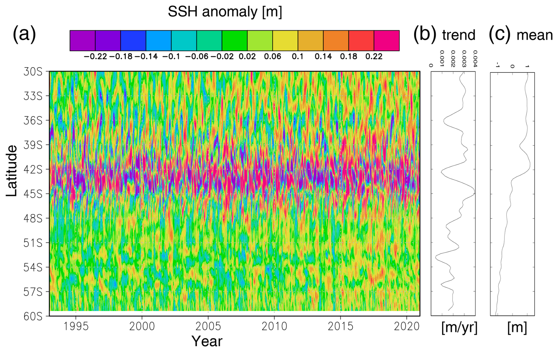
Figure A3 (a) Daily time series of the sea surface height anomalies measured by satellite altimeter along the 57.625° S meridian. Least squares fitting at each latitude yielded profiles of (b) trend and (c) mean.

Appendix B: Additional figure

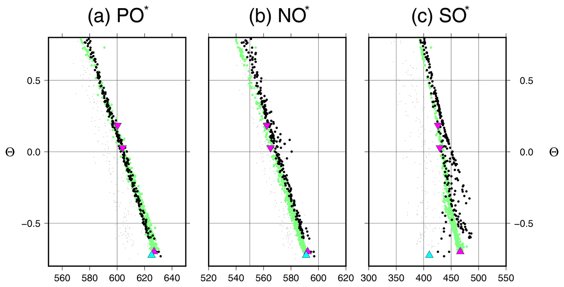
Figure B1 Pseudo-tracers PO${}^{*}=\mathrm{170}[$PO₄]+[O₂] (a), NO${}^{*}=\mathrm{10.625}[$NO₃]+[O₂] (b), and SO${}^{*}=\mathrm{1.66}[$SO₄]+[O₂] (c) plotted against Conservative Temperature. The green points show deep (γⁿ>28.0) data on I06S (30° E). The black points show deep (γⁿ>28.0 and depth greater than 3000 dbar) data on I07S. The grey dots show data from the KH19 cruise. The source waters used in the mixing analysis are indicated by triangles: LCDWs by inverted magenta triangles (PO${}^{*}=\mathrm{600}$, NO${}^{*}=\mathrm{562}$, SO${}^{*}=\mathrm{426}$ for LCDW1; PO${}^{*}=\mathrm{601}$, NO${}^{*}=\mathrm{565}$, SO${}^{*}=\mathrm{430}$ for LCDW2), WSDW by the magenta triangle (PO${}^{*}=\mathrm{627}$, NO${}^{*}=\mathrm{592}$, SO${}^{*}=\mathrm{467}$), and CDBW by the cyan triangle (PO${}^{*}=\mathrm{625}$, NO${}^{*}=\mathrm{591}$, SO${}^{*}=\mathrm{410}$).