Blank variability in coulometric measurements of dissolved inorganic carbon

Marine dissolved inorganic carbon (DIC) is by far the largest pool of carbon in the Earth surface system that exchanges with the atmosphere on human-relevant timescales. Measurements of DIC are therefore necessary to study the changing marine carbon cycle. The most accurate routine DIC measurement method is coulometry. In this method, the signal detected by a coulometer for each measurement must be corrected for background noise, which is termed the blank. The current best practice recommendation is to measure the blank once per analysis session and use this constant value to correct all measurements. However, calculating the blank for each measurement separately shows that the blank sometimes changes during analysis sessions. Correcting measurements to a constant blank when the blank is actually changing leads to an apparent drift in DIC results and therefore lower accuracy. Here, we propose an alternative method for coulometer blank corrections in which the blank is calculated on a per-measurement basis. The per-measurement blank values are then fitted to a smoothing function to determine a set of fitted blank values with which the measurements are corrected. We test the three different approaches (constant, per-measurement and fitted) by applying them to 263 measurements of a laboratory internal standard conducted during 89 analysis sessions over ∼ 7 years. Switching from the constant blank to either the per-measurement or fitted blank improves the precision from 1.85 to 1.31 µmol kg⁻¹. This improvement is statistically significant and important relative to the climate-quality uncertainty target for DIC measurements of ±2 µmol kg⁻¹. Using the fitted blank rather than per-measurement blank eliminates a number of outliers, notably reducing the total range and kurtosis of the residuals. A free and open source Python package (koolstof) has been made available to perform fitted blank corrections for some common coulometer data types. We recommend that in future coulometric DIC analyses, per-measurement blanks should be routinely calculated as part of the quality control process and the fitted blank method applied either as standard or when a changing blank is observed.

1 Introduction

Carbon in the Earth surface system is divided across a number of different pools, including the atmosphere, vegetation and soils on land, and the ocean. By far the largest of these pools is marine dissolved inorganic carbon (DIC), which at 37 000 Gt-C is 4–5 times larger than all the other pools combined, and which is growing by 2.9 ± 0.4 Gt-C yr⁻¹ from anthropogenic carbon dioxide (CO₂) uptake (Friedlingstein et al., 2025). Accurate measurements of marine DIC are therefore critical for understanding the changing global carbon cycle. An uncertainty in DIC of ±2 µmol kg⁻¹ (i.e., ∼ 0.1 %) or better, referred to as the climate-quality goal, is considered necessary in order to reliably quantify long-term (decadal) trends driven by anthropogenic CO₂ (Newton et al., 2015).

DIC is defined as the sum of the aqueous CO₂, carbonic acid, bicarbonate and carbonate ion substance contents (Zeebe and Wolf-Gladrow, 2001):

$$\begin{array}{}\text{(1)}& \mathrm{DIC}=\left[{\mathrm{CO}}_{\mathrm{2}}\left(\mathrm{aq}\right)\right]+\left[{\mathrm{H}}_{\mathrm{2}}{\mathrm{CO}}_{\mathrm{3}}\right]+\left[{\mathrm{HCO}}_{\mathrm{3}}^{-}\right]+\left[{\mathrm{CO}}_{\mathrm{3}}^{\mathrm{2}-}\right]\end{array}$$

The [H₂CO₃] term is negligibly small and therefore usually ignored or combined with [CO₂(aq)]. The relative proportions of the DIC components are sensitive to pH, with greater [CO₂(aq)] at lower pH. DIC is most often measured by acidifying a sample, converting all DIC components to CO₂(aq). This is then extracted by bubbling through with an inert carrier gas (e.g., nitrogen), which carries the CO₂ to a detector (Dickson et al., 2007).

The most accurate routine DIC measurements are conducted with a coulometer (Huffman, 1977; Johnson et al., 1985, 1987, 1993; Dickson et al., 2007). In this method, the gas stream is released into a coulometric cell containing an ethanolamine-based absorbent and thymolphthalein indicator. Hydroxyethylcarbamic acid forms on reaction with CO₂, lowering the pH of the solution and thus the indicator's blue colour to almost colourless. An electrical current is then applied across the cell, which neutralises the acid by forming hydroxide ions at the platinum cathode. The integrated electrical current, termed the counts, required to return the cell solution to its original colour is proportional to the amount of CO₂ that was delivered to the cell, following Faraday's first law of electrolysis. However, coulometers typically record a background level of counts when no CO₂ is passing through, termed the blank. The origin of the blank remains uncertain, but it is thought to be a property of the coulometer cell itself, rather than arising from CO₂ contamination (Johnson et al., 1985). Nevertheless, the integrated counts must be corrected for the blank to accurately calculate DIC.

The current best-practice recommendation to quantify the blank is to measure the coulometer response for a 10 min period when no sample is passing through, usually at the start of each analysis session, and to use this constant value to correct all measurements in the session (Johnson et al., 1993; Dickson et al., 2007). However, a freshly made cell often has a high blank that decreases to a relatively stable lower value (Johnson et al., 1985), so the analyst must judge when this stable behaviour has been reached before measuring the blank. This approach also does not detect if and how the blank changes through an analysis session. Unaccounted-for changes in the blank would present as an apparent drift in the final DIC results, reducing measurement accuracy. Repeated measurements of a reference standard are sometimes used to correct for coulometer drift (e.g., Tanhua et al., 2013), but if a component of the drift were due to a changing blank, then it would be preferable and more accurate to correct for this directly.

Here, we present an alternative approach of determining the coulometer blank for each measurement separately, which accounts for changes through each analysis session. A free and open-source Python package (koolstof; Humphreys, 2025) has been made available to carry out and visualise this processing step. We show how this approach can affect the reproducibility of DIC measurements by application to a real dataset of seawater measurements from our laboratory.

2 Methods

2.1 Quantifying per-measurement blanks

In a DIC measurement of a ∼ 20 mL seawater sample, the coulometer cell current (counts) is typically integrated over a period from 8 to 20 min. Depending on the instrument, the integration time may be fixed, or it may vary per sample, for example finishing after the counts per minute stay below some threshold for a certain duration. However, the DIC in the sample usually contributes to the counts only for up to the first 5–6 minutes. After this, the current intermittently applied across the coulometer cell can be considered to represent the blank. The same period can usually be used to assess the per-measurement blank for all measurements, unless the samples have significantly different DIC values, with higher-DIC samples taking longer to be titrated.

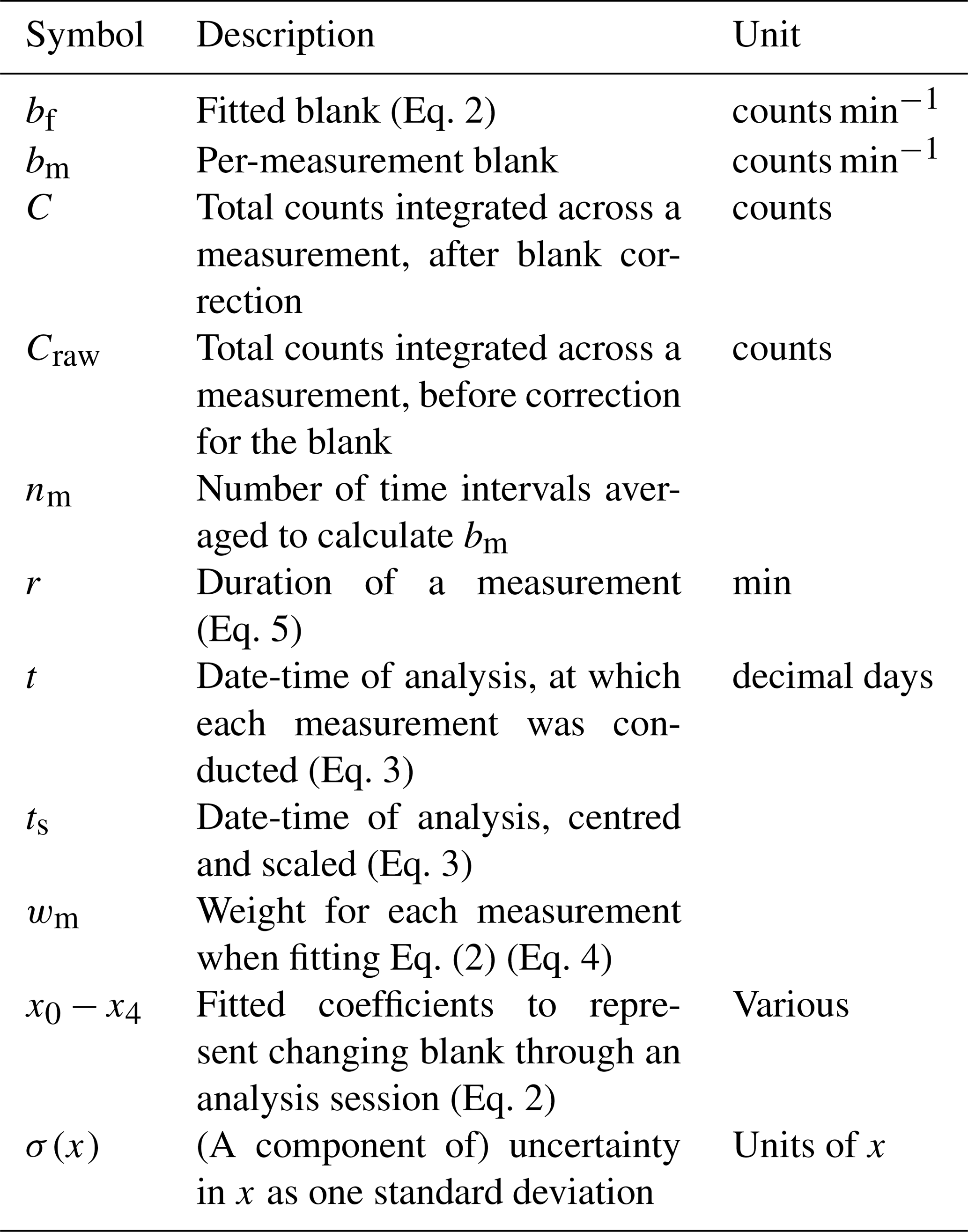
To quantify the per-measurement blank (b_m – see Table A1 for a summary of all symbols used here), the final period of each measurement that represents the blank must be identified. When plotting the coulometer increments against the titration time (i.e., counts per unit time, here per minute), there should be a period of several minutes (at least 3, but ideally 5 or more) towards the end of each measurement where there is no trend in the increments (Fig. 1). If not, then the integration period should be extended, regardless of whether the blank correction procedure described here is being followed. The per-measurement blank is calculated as the mean increments during the identified final period. The standard deviation of the increments during this period, σ(b_m), and the number of intervals being averaged, n_m, are calculated for weighting the measurements during the fitting step. It is also useful to review individual measurements with anomalously high standard deviations during quality control.

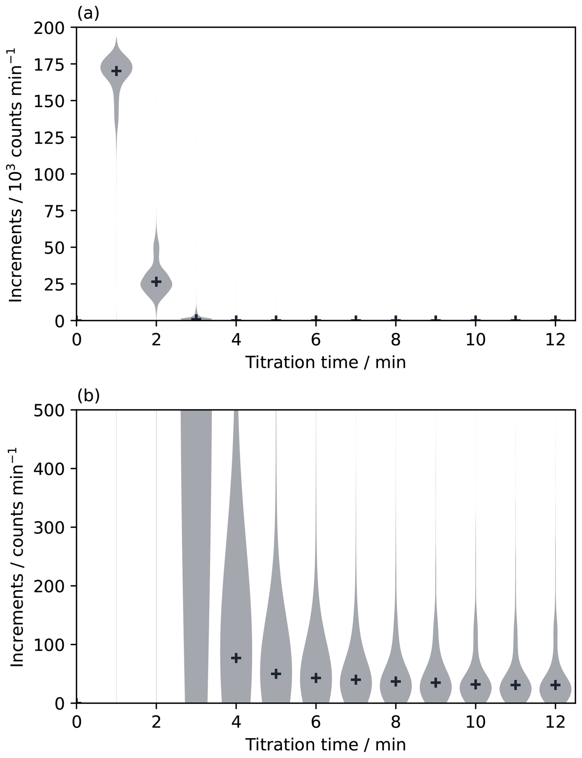
Figure 1 Violin plots of the distributions of coulometer increments (i.e., counts per minute) across our entire test dataset (Sect. 2.6). The widths of the shaded areas show the proportion of data points at each number of increments. Plus symbols show the median value for each minute. Both panels show the same data: (a) covers the full range of increments while (b) zooms in on the lower counts observed towards the end of each titration, which can be considered to represent the blank. In the analysis presented here, we used the increments from minute 6 onwards to calculate the per-measurement blanks. Not all titrations were run for 12 min; some were stopped after 8 or 10 min.

2.2 Smoothed fitting

The fitting procedure should be carried out separately for each analysis session. An analysis session consists of a set of measurements all conducted with the same coulometer cell and chemicals, so a separate analysis session begins each time the chemicals in the coulometer cell are replaced.

Once all per-measurement blanks have been calculated for an analysis session, they are fitted to an equation of the form

$$\begin{array}{}\text{(2)}& b_{\mathrm{f}}\left(t_{\mathrm{s}}\right)=max\left(x_{\mathrm{0}}+x_{\mathrm{1}}{t}_{\mathrm{s}}+x_{\mathrm{2}}\exp \left({\displaystyle \frac{x_{\mathrm{3}}-t_{\mathrm{s}}}{x_{\mathrm{4}}}}\right),\mathrm{0}\right)\end{array}$$

where t_s is the centred and scaled analysis time:

$$\begin{array}{}\text{(3)}& t_{\mathrm{s}}={\displaystyle \frac{t-\mathrm{mean}\left(t\right)}{\mathrm{std}\left(t\right)}}\end{array}$$

where t is the time at which each analysis was conducted in decimal days. Centring and scaling the analysis time with Eq. (3) is necessary for an iterative solver to reliably converge on a solution for Eq. (2). The coefficients x₀−x₄ are found as the weighted least-squares best fit values, with the weight for each measurement (w_m) calculated as

$$\begin{array}{}\text{(4)}& w_{\mathrm{m}}={\displaystyle \frac{\sqrt{n_{\mathrm{m}}}}{\mathit{\sigma }\left(b_{\mathrm{m}}\right)}}\end{array}$$

The fit should be visually inspected. Sometimes certain outliers need to be ignored in order to generate a fit that follows the main pattern of the samples well. We select these outliers manually.

Equation (2) was designed to be able to capture the patterns in blank variability that we have most commonly observed, specifically, an initial exponential decrease, followed by a period where the blank is either constant or follows a linear trend (Fig. 2a). However, Eq. (2) is empirical, and a different fitting function could be used instead if Eq. (2) did not effectively capture the blank variability for a particular dataset. For example, sometimes it may be appropriate to use a linear fit without the initial exponential change, thus setting x₂ to zero.

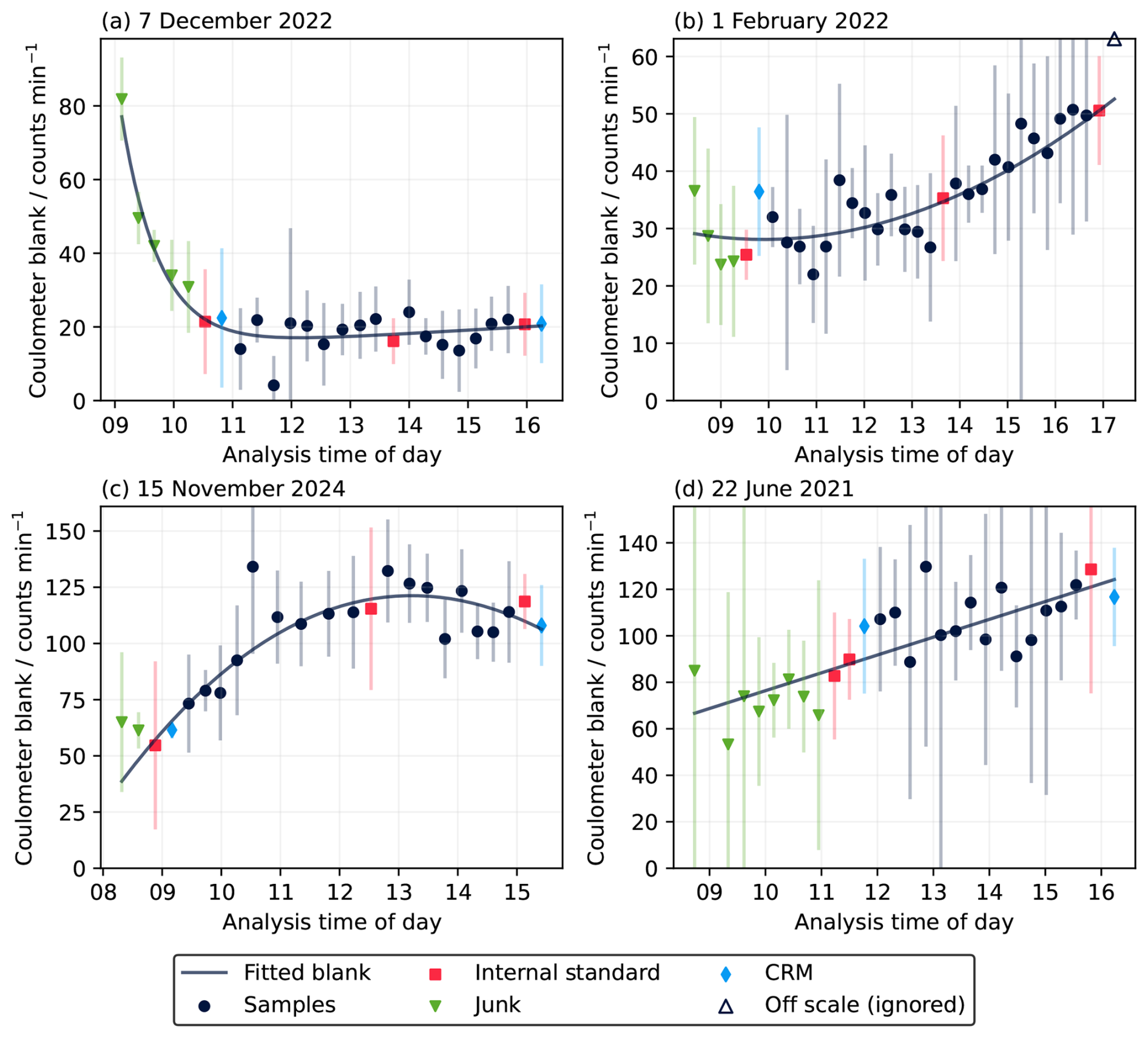
Figure 2 Equation (2) fitted to per-measurement blanks for four different analysis sessions in our test dataset (red squares; Sect. 2.6). Error bars show the standard deviation in the blank at each point, σ(b_m). (a) Shows the ideal behaviour of high initial blank which declines to a stable, roughly constant value after a few hours. (b) and (c) show concave and convex patterns that are sometimes observed but can still be fitted by Eq. (2); (b) includes an off-scale point that was excluded for fitting. (d) shows an example where ignoring the exponential term in Eq. (2) gives a better fit (i.e., linear). Equivalent plots for all analysis sessions in the test datasets are available in the Supplement.

Once the best-fit coefficients have been found, the root-mean-square deviation (RMSD) between the per-sample blanks and the fitted line is calculated as an estimate of the uncertainty in the blank for the corresponding analysis session, denoted σ(b_f).

2.3 Blank correction

The blank correction is applied to each titration after fitting the coefficients x₀−x₄ in Eq. (2):

$$\begin{array}{}\text{(5)}& C=C_{\mathrm{raw}}-r{b}_{\mathrm{f}}\left(t_{\mathrm{s}}\right)\end{array}$$

where r is the titration duration, C is the corrected counts, and C_raw the total counts integrated across the titration. The corrected counts C should be directly proportional to DIC and can be converted into DIC values with Faraday's law or by calibration to some reference standard (e.g., gas loops or sodium carbonate solutions; Dickson et al., 2007).

2.4 Blank uncertainty

We calculate the uncertainty in the corrected counts C due to the blank as

$$\begin{array}{}\text{(6)}& \mathit{\sigma }\left(C\right)=r\mathit{\sigma }\left(b_{\mathrm{f}}\right)\end{array}$$

where σ(b_f) is the RMSD of the residuals between b_f and b_m (Sect. 2.2). If σ(C) is converted into a percentage, then it is equal to the corresponding component of uncertainty in DIC as a percentage. Alternatively, the uncertainty in DIC due to the blank can be calculated in DIC units as

$$\begin{array}{}\text{(7)}& \mathit{\sigma }\left(\mathrm{DIC}\right)={\displaystyle \frac{\mathrm{DIC}}{C}}r\mathit{\sigma }\left(b_{\mathrm{f}}\right)\end{array}$$

2.5 Python package

We have prepared a free and open source Python package called koolstof to help apply and visualise fitted blank corrections. The analysis here was conducted using koolstof v1.0.0-b.3 (Humphreys, 2025). The code is hosted on GitHub (https://github.com/mvdh7/koolstof/) and the package can be installed from the Python Package Index (https://pypi.org/, last access: 20 November 2025) or through conda-forge (https://conda-forge.org/, last access: 20 November 2025). Koolstof makes use of several other open source Python packages, primarily NumPy (Harris et al., 2020), SciPy (Virtanen et al., 2020), pandas (McKinney, 2010) and Matplotlib (Hunter, 2007).

2.6 Test dataset

To compare the different blank correction approaches, we applied them all to a test dataset. Within a total dataset of 2809 measurements, 280 measurements of a laboratory internal standard were conducted across 95 separate analysis sessions over a period of ∼ 7 years (June 2018 to June 2025). All measurements were carried out by the same analyst and using the same DIC extraction instrument (VINDTA 3C #015, Marianda, Germany) and coulometer (CO₂ Coulometer 5011, S/N AHR-8912-V, UIC Inc., USA). Counts were recorded each minute during each titration. 11 outliers resulting from various analytical problems were removed, and a further 6 measurements were unusable because they were the only usable measurement in their analysis session, leaving a final test dataset of 263 measurements across 89 analysis sessions which was used for the analysis described here (Supplement Fig. S1). The test dataset titrations were each run from 8 to 18 min, with the majority (160 of the test dataset, 1949 of all measurements) being run for 12 min. Values from 6 min onwards were considered to represent the blank (Fig. 1) and thus calculate b_m (Sect. 2.1).

The internal standard was subsampled shortly before each measurement, drawn from a large vat (∼ 300 L) of natural low-nutrient seawater that had been filtered (Sartorius Sartobran^® P Sterile Midicaps^® 0.45 + 0.2 µm) upon collection. The vat was replenished several times throughout the course of these measurements with seawater collected from the Mediterranean Sea or North Atlantic Ocean, and it was not perfectly sealed off from the surrounding air, so its DIC varied through the 7-year period (Fig. S1). However, it was stable on timescales of up to a few weeks and always consistent within each analysis session (i.e., for up to 10 h). The internal standard measurements were spread within each analysis session, usually with one towards the start and one towards the end, and sometimes with additional measurements in between.

Three different blank correction approaches were applied to the measurements: (1) constant blank for each session; (2) per-measurement blank, using each sample's own b_m value directly; (3) fitted blank b_f with Eq. (2). The resulting DIC values were normalised to the mean for each analysis session to account for the internal standard's changing DIC through time and compiled for statistical comparisons.

2.7 Statistical tests

Despite removing large outliers, there were still a number of outliers in the normalised DIC values relative to a normal distribution, especially for the constant and per-measurement blank correction approaches, so the statistical tools needed to account for this. The significances of the differences between the variances for the three distributions were tested using the median version of the Brown-Forsythe test (Levene, 1960; Brown and Forsythe, 1974), which was selected because it is robust against outliers. For the same reason, the spreads of the data were computed using the S_n spread statistic (Rousseeuw and Croux, 1993), which is equal to a standard deviation if data are normally distributed. Kurtosis was computed using Fisher's definition (i.e., zero for a normal distribution).

3 Results and discussion

3.1 Blank fits

The standard pattern of blank variability is a high initial value that decreases over a few hours before levelling off to a constant value (Johnson et al., 1985). This pattern is fit well by Eq. (2) (Fig. 2a), which also provides a good fit to most other patterns of blank variability that we observed (e.g., Fig. 2b–d). In some cases, the exponential part of the equation should probably be excluded, resulting in a linear fit (e.g., Fig. 2d).

3.2 Comparison of the approaches

Switching from a constant blank to either the per-measurement or fitted blank significantly improves the precision of the test dataset (Table 1; Fig. 3). As well as being statistically significant, the improvement in precision is of an important magnitude (Table 2; Fig. 3) relative to the total uncertainty target for climate-quality DIC measurements of ± 2 µmol kg⁻¹ (Newton et al., 2015): the constant blank gives an S_n spread of 1.85 µmol kg⁻¹ (i.e., 0.09 %), as opposed to 1.31 µmol kg⁻¹ (0.06 %) for the per-measurement and fitted blank approaches. The approaches with a varying blank therefore leave more space in the uncertainty budget for other uncertainty components not included in these measurements.

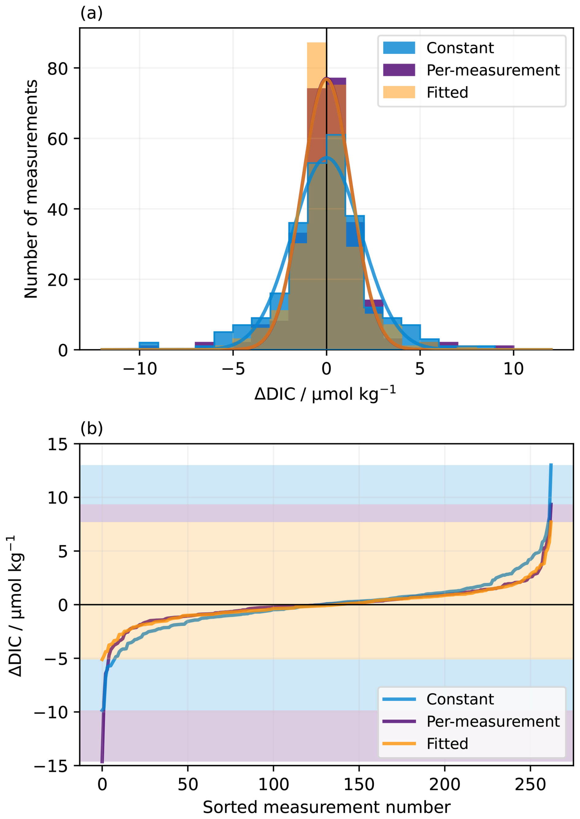
Figure 3 Distributions of the internal standard DIC normalised to each analysis session's mean value (ΔDIC) using the constant, per-measurement and fitted blank corrections. In (a), the curves follow normal distributions with standard deviations equal to the S_n spread for each distribution (Table 2) so that they follow the main pattern of the data rather than being overly influenced by outliers. The histogram bars are semi-transparent. (b) Cumulative histogram of the same distributions as in (a), with measurements sorted in order of ΔDIC on the horizontal axis, and the shaded areas highlighting the total range of each distribution (Table 2).

Table 1 Results of median Brown-Forsythe (BF) tests comparing the variances of the normalised internal standard measurements under the constant, per-measurement and fitted blank approaches. The null hypothesis is that the variances of the two distributions are the same, so a low p-value (e.g., < 0.05) indicates that the null hypothesis can be rejected and thus the variances are considered to be significantly different.

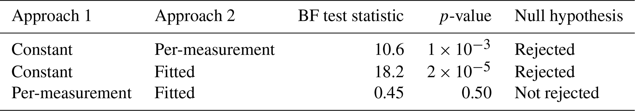
Table 2 Summary statistics for the normalised distributions of DIC with the blank corrected using the different approaches.

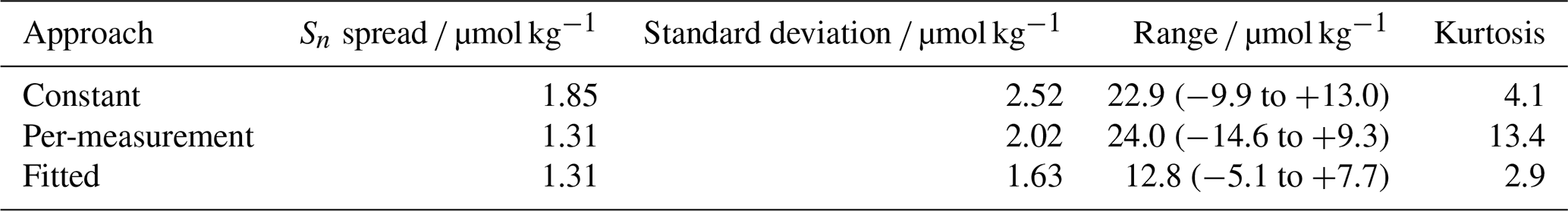
Although the per-measurement and fitted blank approaches have similar distributions of residuals and their variances are not significantly different (Table 1), the per-measurement approach has much larger outliers, which disappear when using the fitted blank (Fig. 3). This difference is masked by the S_n spread statistic, which is relatively robust to outliers, but can be clearly seen in the standard deviation, range and kurtosis of the residuals for the different approaches, which are all lowest with the fitted blank (Table 2). The kurtosis is particularly high for the per-measurement approach, which we interpret to mean that the few minutes available to assess the blank at the end of each measurement are not always enough to accurately constrain its blank, so the fitting allows information from the preceding and following measurements to also influence the value, making it more robust.

3.3 When to use fitted blanks

A significantly drifting blank is a sign that there is a problem with the sample extraction or coulometer system. The first course of action should be to pause measurements until this can be resolved. Such problems can arise for many reasons, including electrical faults, needing to clean or replace the coulometer cell glassware, or using old or contaminated coulometer cell solutions (Johnson et al., 1985, 1987). It is not recommended that the fitted blank approach be used indefinitely instead of fixing the root problem. Nevertheless, sometimes these issues are not identified until after a batch of measurements has been conducted, and, due to gas exchange, DIC samples cannot be reanalysed once the sample bottles have been opened. The fitted blank approach can allow climate-quality DIC measurements still to be obtained in this scenario, and it can further improve the precision of DIC measurements even when a constant blank would already deliver climate-quality data.

We recommend that per-measurement blanks should always be calculated and checked for signs of drift. Although it is not necessary to use a fitted blank if drift is absent or negligible, the fitted blank will return a result that is virtually identical to using a constant blank in this case, so there is no disadvantage to always using the fitted blank.

While Eq. (2) usually returns a good fit that captures the form of the blank variability well, it may fail or provide an unsuitable result that does not follow the pattern of the data in some particular cases. It is therefore essential to visually inspect the per-measurement blanks together with the fitted line for each analysis session and adjust where necessary rather than blindly following the fit.

Our experience shows that using the fitted blank approach often, but not always, eliminates apparent drift in coulometer DIC measurements. It is therefore advisable to still measure some sort of reference material at least at the start (after the system has stabilised) and end of each analysis session as a check on whether there is some other source of drift in the measurements.

3.4 Uncertainty from the blank

The distribution of uncertainties in corrected counts (and therefore also in DIC) based on Eq. (6) is shown in Fig. 4. This varies between analysis sessions based on how closely the per-measurement blanks match the fitted blank curve (i.e., the RMSD of the residuals, σ(b_f)). The majority (76 %) of measurements have a calculated uncertainty due to the blank of less than 0.1 %, with a median of 0.07 %. This suggests that variability in the blank in our test dataset is a major uncertainty component in the overall precision of the test dataset measurements of ∼ 0.06 % (Sect. 3.2). Therefore, taking practical steps to reduce the blank and make it more consistent (Sect. 3.3) would probably lower the overall uncertainty of future measurements with the instrument used to generate the test dataset.

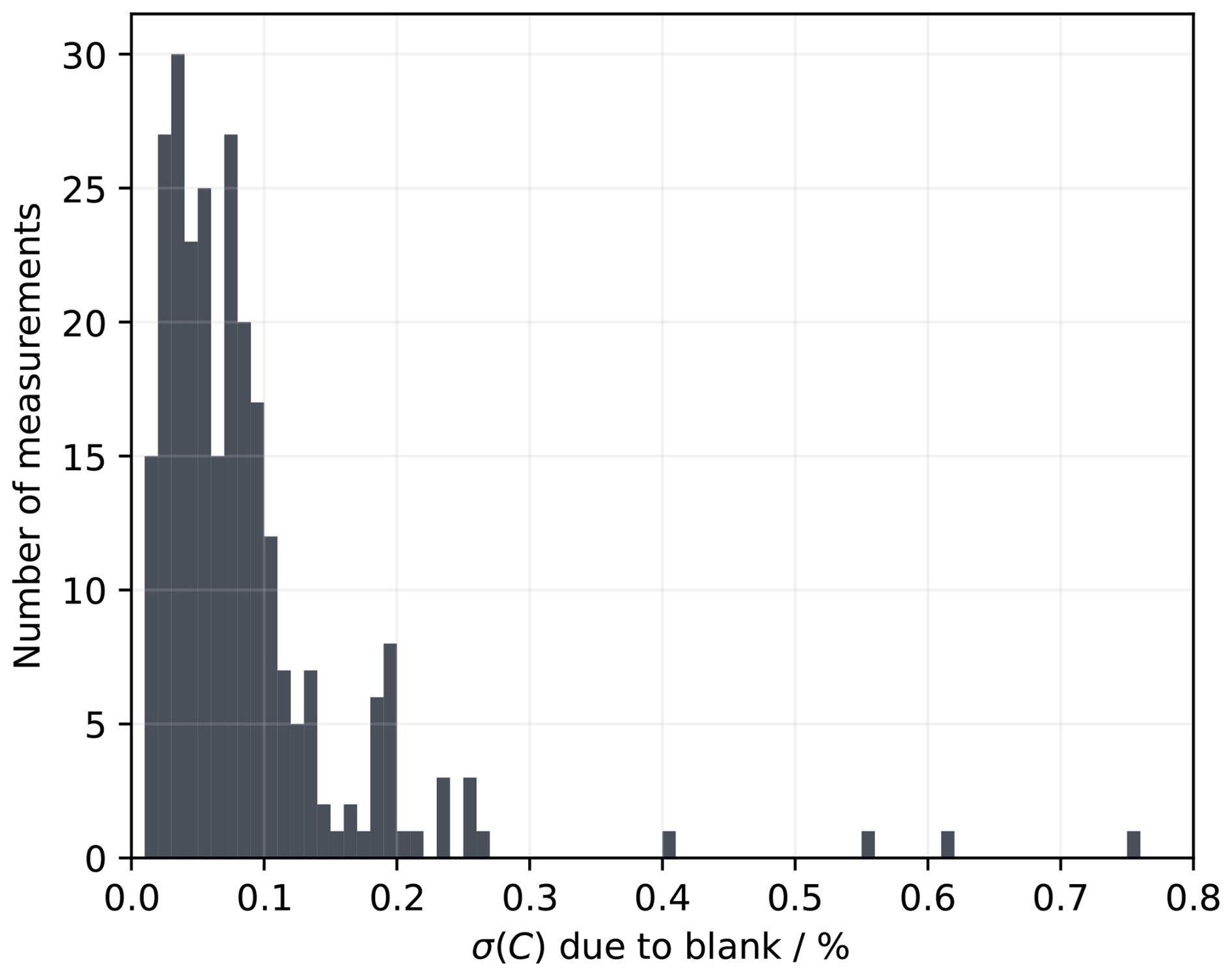
Figure 4 Distribution of uncertainties in corrected counts (C) for the test dataset as a percentage, following Eq. (6).

4 Conclusion

The coulometer blank can be assessed separately for each measurement and this is a useful calculation that should be incorporated into standard operating procedures as a routine quality control check. If changes in the blank are observed, then using a variable blank computed from all measurements can significantly improve the precision of coulometric DIC data relative to using a constant value, and using a fitting function to smooth the per-measurement blank across an analysis session can further improve precision by reducing the occurrence of outliers. However, significant changes in the blank indicated an underlying problem with the measuring system, which the analyst should endeavour to identify and fix rather than rely indefinitely on the approach presented here.

Appendix A: Glossary of symbols

Table A1 Symbols used in this manuscript.