The effect of storms on the Antarctic Slope Current and the warm inflow onto the southeastern Weddell Sea continental shelf

Storms have been suggested to drive enhanced southward transport of modified Warm Deep Water (mWDW) towards the Filchner Ice Front in the southern Weddell Sea. This region is a known location of dense bottom water production and is thus tightly linked to the global climate system. However, increased heat transport could lead to higher ice shelf melt rates and disrupt dense water production. The role of storms and wind forcing in enhancing the southward heat transport is therefore of interest. We utilize observational records spanning up to four years of data from a network of moorings deployed in the Filchner Trough region to investigate how the regional ocean circulation responds to storm events. We find that about 70 % of the storm events that (i) last sufficiently long (longer than 5.7 d), (ii) have a large enough accumulation of ocean surface stress anomaly throughout the storm (larger than 0.9 N m⁻² d⁻¹), and (iii) are severe enough at their peak intensity (maximum stress above 0.5 N m⁻²) lead to a significant increase in the speed of the Antarctic Slope Current (ASC) just upstream of Filchner Trough while roughly 25 % of the identified events also cause increased southward current speed on the shelf at depths where mWDW is expected to be present during the summer and autumn. At the southernmost mooring (76° S) storm-driven responses are observed mainly during the latter part of the record (mid-2019 to early 2021). This interannual variability in storm response indicates a potential dependency on background hydrography and circulation that remains to be fully explained. This study highlights the potential importance of storms for southward heat transport: an accelerated circulation on the shelf increases the likelihood for warm summer inflow to reach the ice shelf front and cavity before the heat is lost to the atmosphere through winter convection.

1 Introduction

Strong ocean surface stress events – hereafter referred to as storms – have been suggested (Darelius et al., 2016; Dundas et al., 2024) to cause enhanced southward transport of modified Warm Deep Water (mWDW, $\sim -\mathrm{1.5}$ to 0.0 °C, Nicholls et al., 2009) across the continental shelf in the southeastern Weddell Sea. This shelf is currently characterized as a cold, dense shelf region (Thompson et al., 2018) with an outflow of dense Ice Shelf Water through Filchner Trough (Foldvik et al., 2004). Southward intrusions of mWDW, originating from the open ocean north of the continental shelf break (Årthun et al., 2012), are mostly limited to the summer season when the thermocline at the shelf break is shallow (e.g., Darelius et al., 2024b; Årthun et al., 2012). These deep intrusions of mWDW onto the continental shelf typically fill the water column below 300 m depth, creating a thick layer of warm waters below the cold surface waters (e.g., Steiger et al., 2024; Årthun et al., 2012). The warm water propagates southward throughout autumn and reaches roughly halfway south to the Filchner Ice Front several months later (Steiger et al., 2024; Ryan et al., 2017; Sallée et al., 2024). Darelius et al. (2016) suggested that storms can drive particularly far-reaching intrusions of warm water, as they observed coincident events of strong, short-lived anomalies in wind speed and enhanced ocean currents carrying mWDW southward along the eastern flank of Filchner Trough. It has further been suggested that if mWDW consistently enters the Filchner Ice Shelf cavity along this path the system could shift from a cold to a warm regime with dramatically increased basal melt rates in the future (Hellmer et al., 2012, 2017). Enhanced basal melt affects deep water production and the hydrography on the continental shelf, as well as sea level through reduced buttressing of continental ice flow into the ocean, and thus is of global importance (Orsi et al., 1999; Marshall and Speer, 2012; Jacobs, 2004). Given these implications, this study aims to deepen our understanding of how storms affect the circulation and the southward heat transport in the Filchner Trough region.

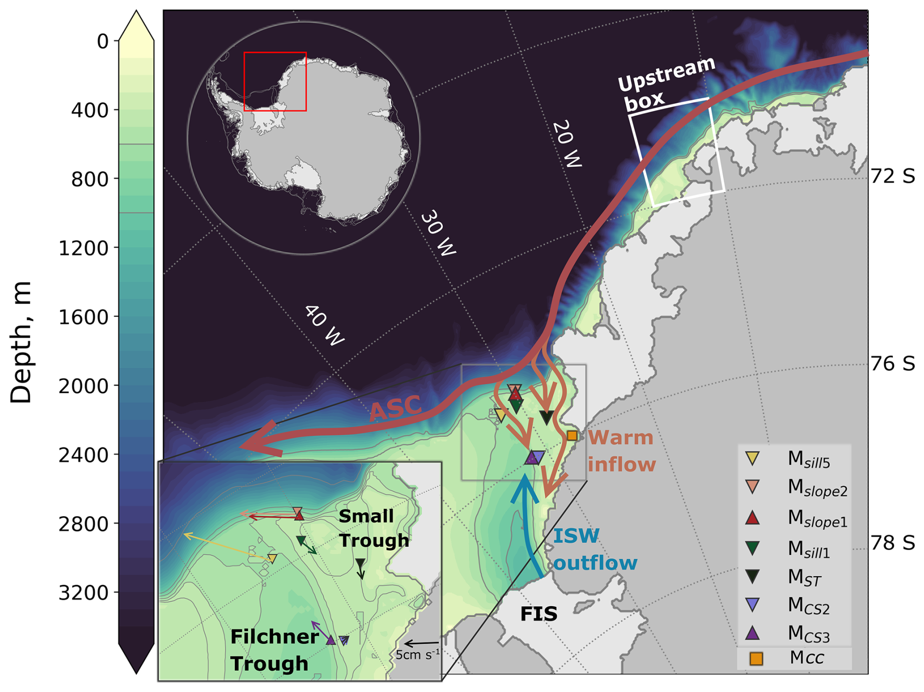
Figure 1 Map over the study area showing the mooring locations (colored markers), the main currents (Nicholls et al., 2009; Darelius et al., 2014) and the “Upstream box” used to estimate the ocean surface stress. The bathymetry (color and gray contours) and the floating ice shelves (light gray) are from Bedmap2 (Fretwell et al., 2013). Filchner Trough, the Small Trough, Filchner Ice Shelf (FIS), the Antarctic Slope Current (ASC), the warm inflow and the Ice Shelf Water (ISW) outflow are labeled. The red box in the upper inset indicates the study region. The lower inset shows the vertically averaged current at the mooring locations.

The strong horizontal density gradient characterizing the Antarctic Slope Front (ASF), separates the cold shelf waters from the warm water of the open ocean (e.g., Gill, 1973; Jacobs, 1991; Thompson et al., 2018). The persistent westward wind field (Hazel and Stewart, 2019) and the ASF is associated with the strong westward Antarctic Slope Current (ASC, e.g., Thompson et al., 2018; Gill, 1973). The ASF and the ASC thus make up a strongly coupled system. Wintertime easterlies lead to Ekman convergence and coastal downwelling that act to steepen the ASF and sustain a strong ASC (Thompson et al., 2018). In the Weddell Sea, the ASF relaxes during summer due to weaker wind and stronger surface stratification (Hattermann, 2018; Daae et al., 2017) and allows warm water to access the continental shelf (e.g., Årthun et al., 2012; Ryan et al., 2017; Steiger et al., 2024).

The relationship between the wind, the ASF, and the ASC is different on subseasonal time scales: Strong easterlies associated with storm events increase the sea surface height (SSH) slope through Ekman transport towards the coast, which enhances the barotropic component of the ASC. The storms, however, do not act sufficiently long to steepen the ASF. The increase in the barotropic component of the ASC is the main mechanism by which storms are suggested to enhance the heat transport towards the Filchner Ice Shelf cavity, as it strengthens the circulation on the shelf and accelerates the southward motion of warm waters already present on the continental shelf (Darelius et al., 2016; Dundas et al., 2024). In the current climate, the water column on the shelf is homogenized during winter (Ryan et al., 2017; Sallée et al., 2024), and all heat is lost to the atmosphere. The warm inflow must therefore traverse the roughly 400 km-wide continental shelf during the summer season if it is to reach the ice front and the Filchner Ice Shelf cavity.

The deep Filchner Trough crosscuts the southeastern Weddell Sea continental shelf and acts as a southward gateway for mWDW towards the Filchner Ice Shelf cavity (Fig. 1). At the mouth of Filchner Trough, the ASC bifurcates as the diverging isobaths steer a small branch of the current along the eastern flank of the trough (westernmost orange arrow in Fig. 1, e.g., Nicholls et al., 2009; Foldvik et al., 1985). Part of this southward-flowing current recirculates on the sill and joins the northward flow of Dense Shelf Water (DSW, Daae et al., 2017; Foldvik et al., 2004). The remainder of the current continues south (e.g., Daae et al., 2017; Steiger et al., 2024), advecting warm mWDW southward along the eastern flank of Filchner Trough (e.g., Ryan et al., 2017; Darelius et al., 2016; Daae et al., 2020). Intrusions of mWDW have also been observed further east, as indicated by the two easternmost arrows in Fig. 1 (Steiger et al., 2024; Nicholls et al., 2009; Sallée et al., 2024).

The circulation and hydrography in Filchner Trough changes as the circulation below the Filchner-Ronne Ice Shelf shifts between the “Berkner” and “Ronne” modes of Ice Shelf Water production (ISW, below-freezing temperatures, e.g., Foldvik et al., 2004). The “Ronne”-mode is characterized by large-scale cavity circulation and enhanced outflow of high-salinity Ronne-sourced ISW through Filchner Trough, while the “Berkner”-mode is characterized by more prominent local circulation and locally sourced ISW with lower source salinities (Hattermann et al., 2021; Janout et al., 2021).

Idealized numerical experiments support the hypothesis that storms enhance the southward heat transport by increasing the circulation on the continental shelf (Dundas et al., 2024), but historical mooring records do not consistently show a relationship between southward transport and strong wind (Ryan et al., 2017).

In this paper, we focus on this relationship and investigate the conditions during which storms drive enhanced currents along the slope and into Filchner Trough using up to four-year-long records of concurrent mooring data. First, we present a case study and a composite analysis of the oceanic response to storms and the ambient atmospheric conditions during the storms. We then investigate why some events cause strongly enhanced currents while others do not and finally, we briefly discuss a shift in hydrographic conditions and circulation that occurred during 2019. We, thus, provide new insights into the importance of storm events for the ASC and the circulation on the continental shelf and attempt to determine when and why the events enhance the southward flow east of Filchner Trough.

2 Data and methods

2.1 Mooring records

We analyze velocity records from six moorings in the Filchner Trough region in the southeastern Weddell Sea (Fig. 1). The mooring names indicate their geographic location: M_slope1 (Darelius et al., 2024a) and M_slope2 (Darelius et al., 2023b) were positioned on the the continental slope, just north of the shelf beak, and captured the ASC upstream of Filchner Trough. M_sill5 (Østerhus, 2025) and M_sill1 (Steiger et al., 2024) captured the outflow and inflow across the Filchner Trough sill, respectively. M_ST (Steiger et al., 2024) was located in the trough just east of Filchner Trough, which we refer to as the “Small Trough” (Fig. 1). M_CS2 (Darelius et al., 2023b) and M_CS3 (Steiger et al., 2024) were located on the continental shelf on the eastern flank of Filchner Trough. The mooring locations are shown in Fig. 1, and their deployment details are given in Fig. 2 and Table 1. The mooring records span a varying period between 2017 and 2021, but their velocity records overlap for at least 20 months (Fig. 3).

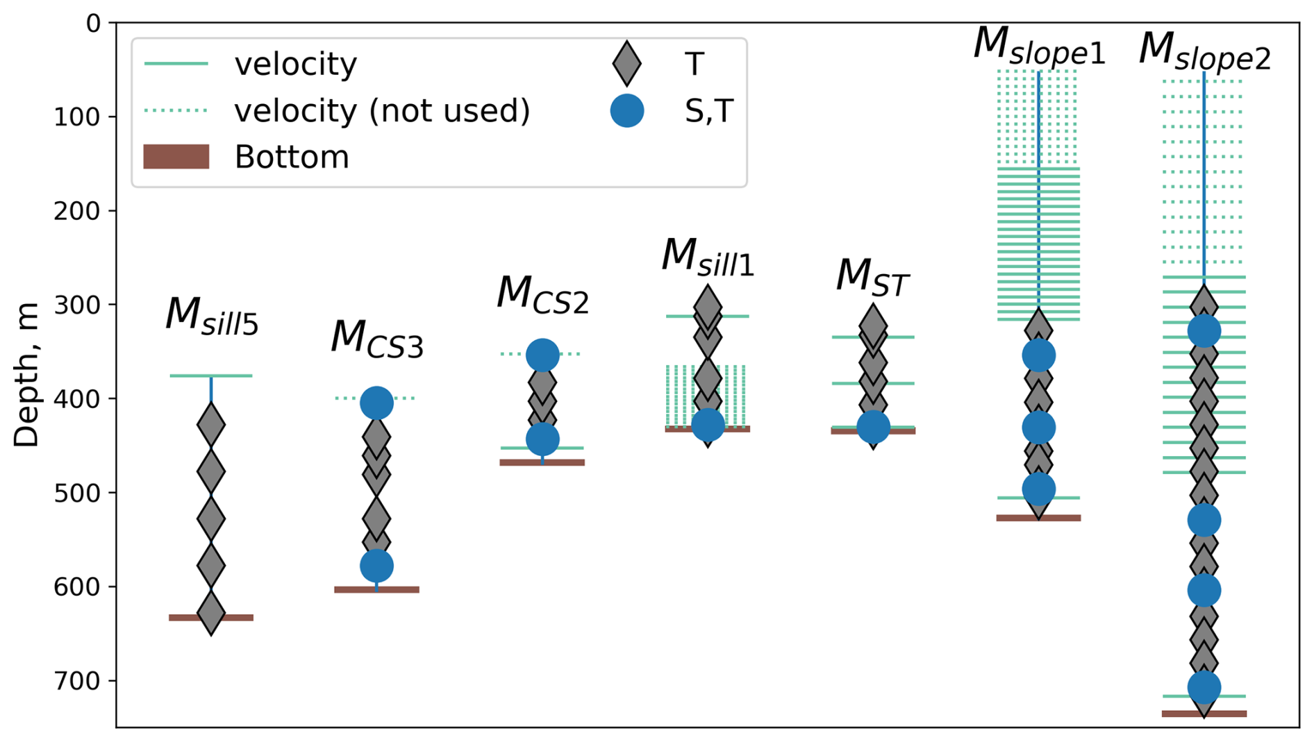
Figure 2 Sketch of the moorings indicating the depths with observational records according to the legend. Tightly spaced turquoise lines indicate ADCP (Acoustic Doppler Current Profiler) bins (M_sill1, M_slope1, and M_slope2), and dotted lines indicate discarded bins.

We rotate the coordinate system at each mooring to align with the mean flow direction, which roughly aligns with the local isobaths (see Fig. 1). A negative sign indicates current speed in the mean flow direction since the mean flows are roughly westward (M_slope1 and M_slope2) and southward (M_sill1 and M_ST). M_CS2 and M_sill5 are the exceptions. At M_sill5 a positive sign indicates current in the main flow direction since it is directed roughly northward. At M_CS2 we align the coordinate system with the local isobaths as the mean current direction shifts (Ryan et al., 2017,  and Fig. 1). After rotation, a negative sign indicates flow towards the southwest. All analyses are carried out using hourly mean velocity records. The moorings M_slope2, M_CS2, and M_sill5 had a sampling interval of two hours for velocity; these records were linearly interpolated onto hourly time steps.

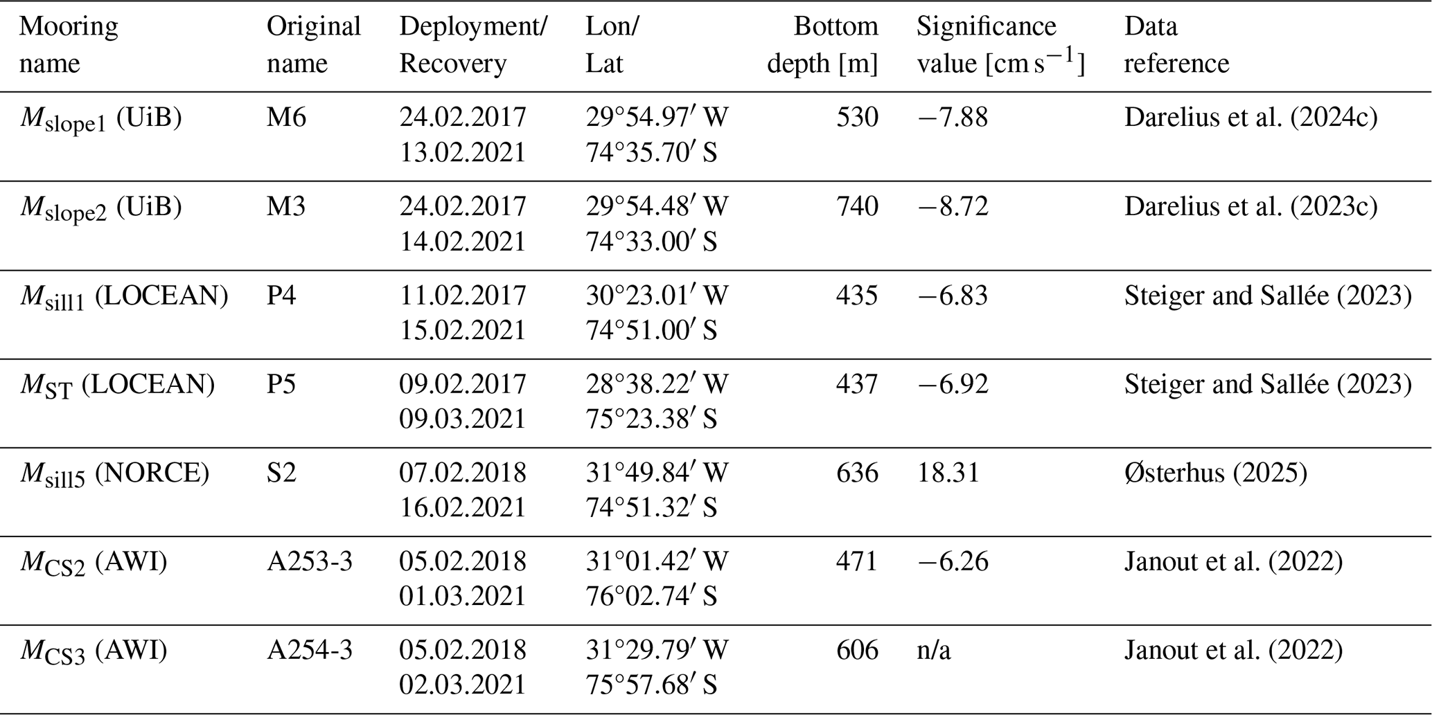
Darelius et al. (2024c)Darelius et al. (2023c)Steiger and Sallée (2023)Steiger and Sallée (2023)Østerhus (2025)Janout et al. (2022)Janout et al. (2022)

Table 1 Overview of the moorings. The indicated significance limits (Sect. 2.5) for storm response are negative for all moorings except M_sill5 because their main observed flow directions have a strong westward or southward component. The significance value at M_sill5 is positive because the main flow direction has a strong northward component. No significance value is indicated for M_CS3 because this mooring is dominated by northward flowing ISW and not used in the storm response analysis. Information about instruments, calibration, and data processing can be found in the indicated data reference. n/a: not applicable.

Where possible, we have used the depth averaged current as we expect the storm response to be mainly barotropic (M_slope1, M_slope2, M_ST). At M_sill1 where the time series from one level is significantly longer than the others we chose to include only data from that level. At mooring M_CS2, the currents at the upper instrument are weak and erratic, and we chose to include only the lower level. The levels included are marked in Fig. 2. At M_slope1 and M_slope2, the data quality of the upper bins is poor during winter due to too few scattering particles, and we've discarded levels with less than 43 % data coverage. Data gaps shorter than six hours are filled by linear interpolation.

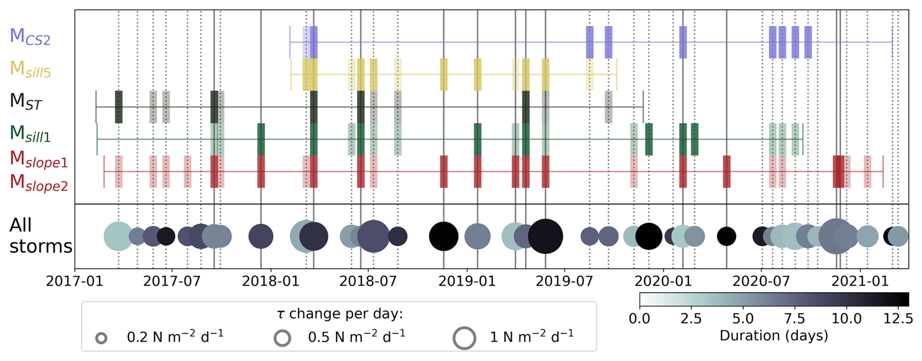
Figure 3 Overview of storms (dashed and solid vertical black lines) and storm responses (colored vertical bars) at the moorings. Horizontal lines show the duration of the mooring records, and dark colored vertical bars indicate a significant storm response. Light vertical bars show storm responses stronger than the 70th percentile of background current increase (see methods Sect. 2.5). Storms with a significant response at both M_slope1 and M_slope2 are shown as solid, black vertical lines. The gray circles indicate the duration (color) and change in ocean surface stress, τ, per day (size) for the identified storms.

While velocity is the main variable in this study, temperature and salinity are used in parts of the analysis. Data from a seventh mooring, M_CS3, located just west of M_CS2 along the eastern slope of Filchner Trough is included when discussing the shift from Ronne to Berkner mode (Fig. 2, Appendix C). We present temperature and salinity as conservative temperature, Θ, and absolute salinity, S_A, following TEOS-10. We use the Gibbs seawater package for Python in conversions (McDougall and Barker, 2011).

2.2 Estimation of ocean surface stress

Ocean surface stress is estimated following Dotto et al. (2018), who estimate the air-ocean stress and ice-ocean stress separately and then combine them as fractions of the sea ice concentration as follows:

$$\begin{array}{}\text{(1)}& {\displaystyle }& {\displaystyle }\mathit{\tau }=\mathit{\alpha }{\mathit{\tau }}_{\text{ice-water}}+(\mathrm{1}-\mathit{\alpha }){\mathit{\tau }}_{\text{air-water}},\text{(2)}& {\displaystyle }& {\displaystyle }{\mathit{\tau }}_{\text{ice-water}}={\mathit{\rho }}_{\mathrm{water}}{C}_{\mathrm{iw}}\left|{\mathit{U}}_{\mathrm{ice}}\right|{\mathit{U}}_{\mathrm{ice}},\mathrm{and}\text{(3)}& {\displaystyle }& {\displaystyle }{\mathit{\tau }}_{\text{air-water}}={\mathit{\rho }}_{\mathrm{air}}{C}_{\mathrm{d}}\left|{\mathit{U}}_{\mathrm{air}}\right|{\mathit{U}}_{\mathrm{air}}.\end{array}$$

Here α is the sea ice concentration, ρ_water=1028 kg m⁻³, ρ_air=1.25 kg m⁻³ are the densities of water and air, and $C_{\mathrm{d}}=\mathrm{1.25}\times {\mathrm{10}}^{-\mathrm{3}}$ and $C_{\mathrm{iw}}=\mathrm{5.50}\times {\mathrm{10}}^{-\mathrm{3}}$ are the drag coefficients between air and ocean and ice and ocean, respectively. U_ice and U_air are the velocities of the ice and the air. The coordinate system is rotated 30° counterclockwise to roughly align with the coast in the Upstream box, and we use the along-slope component of the ocean surface stress in the following analysis.

2.3 Atmospheric and sea ice data

We use 10 m wind velocity, sea ice concentration, and mean sea level pressure from ERA5 (Hersbach et al., 2023). In estimations of the ocean surface stress, τ (Eq. 3) used to identify storm events during the mooring period (Fig. 4), we use three-hourly 10 m wind and sea ice concentration from ERA5 over a region upstream of Filchner Trough (“Upstream box”, Fig. 1). For the maps in Figs. 6 and 9, we use daily averaged output from ERA5. The anomalies of wind velocity and mean sea level pressure in Fig. 6a, b) are referenced to monthly averaged March fields from 1990 to 2023. The sea ice concentration is referenced to the monthly climatology (average over the past 30 years), linearly interpolated onto daily values.

We consider the ERA5 reanalysis a suitable data source for our purposes, as in situ observations are sparse and have limited spatial coverage. Caton Harrison et al. (2022) conducted a detailed comparison of coastal easterlies in three reanalysis products with satellite and in situ observations and concluded that ERA5 has the overall best performance. However, ERA5 underestimates coastal wind and wind speeds exceeding 20 m s⁻¹ in this region (Caton Harrison et al., 2022). It is therefore possible that the strongest wind events identified during our study period are underestimated in magnitude.

The sea ice motion data is from NSIDC (Tschudi et al., 2019) and is available on the 25 km EASE-Grid (NSIDC, 2019). We average over the grid cells that overlap with the Upstream box and apply a rotational matrix to obtain the north and eastward components as described in NSIDC (2024).

2.4 Identification of “storm” events

The following procedure is used to identify events of strong ocean surface stress, “storms”. We de-trend the records of along-slope ocean surface stress and apply a high-pass filter (4th order 180 d Butterworth filter) to remove the seasonality. We then identify storm events as periods when the cumulative stress increases monotonically for more than 12 h and where the total increase is at least 3.5 N m⁻². We thus disregard the shortest and weakest wind events from further analysis, as we do not expect them to cause increased circulation (Dundas et al., 2024). Two storm events are combined if they are less than 15 h apart. This condition is based on idealized model results, which indicate that the circulation increases throughout the storm duration and stays enhanced for a few days after the storm has passed (Dundas et al., 2024). This means that a storm that occurs shortly after another adds momentum to an already enhanced current field.

We use the cumulative ocean surface stress instead of the ocean surface stress directly because of the highly variable nature of the record. Alternatively, we could have used a low-pass filter but that would make the identification of storm start and end imprecise. This is illustrated in Fig. A1a, b.

The “Upstream box” was chosen because upstream wind forcing has been found to drive variability in circulation in this and similar regions on longer timescales (Daae et al., 2018; Lauber et al., 2023). The wind-speed variability in the Upstream box is representative of the conditions in a large area surrounding the box (Fig. A2). A comparison of storm events identified using the Upstream box and a more local box (Fig. A3) gave similar but slightly poorer coherence between storm events and storm response at the slope moorings for the local box. The variability in the ASC strength observed at the slope moorings is relatively high and caused by e.g. baroclinic eddies, continental shelf waves (Jensen et al., 2013), and remote wind forcing (Webb et al., 2019). We therefore do not expect to explain all ASC variability by using our Upstream box, but rather aim to identify regionally forced peaks in ASC strength.

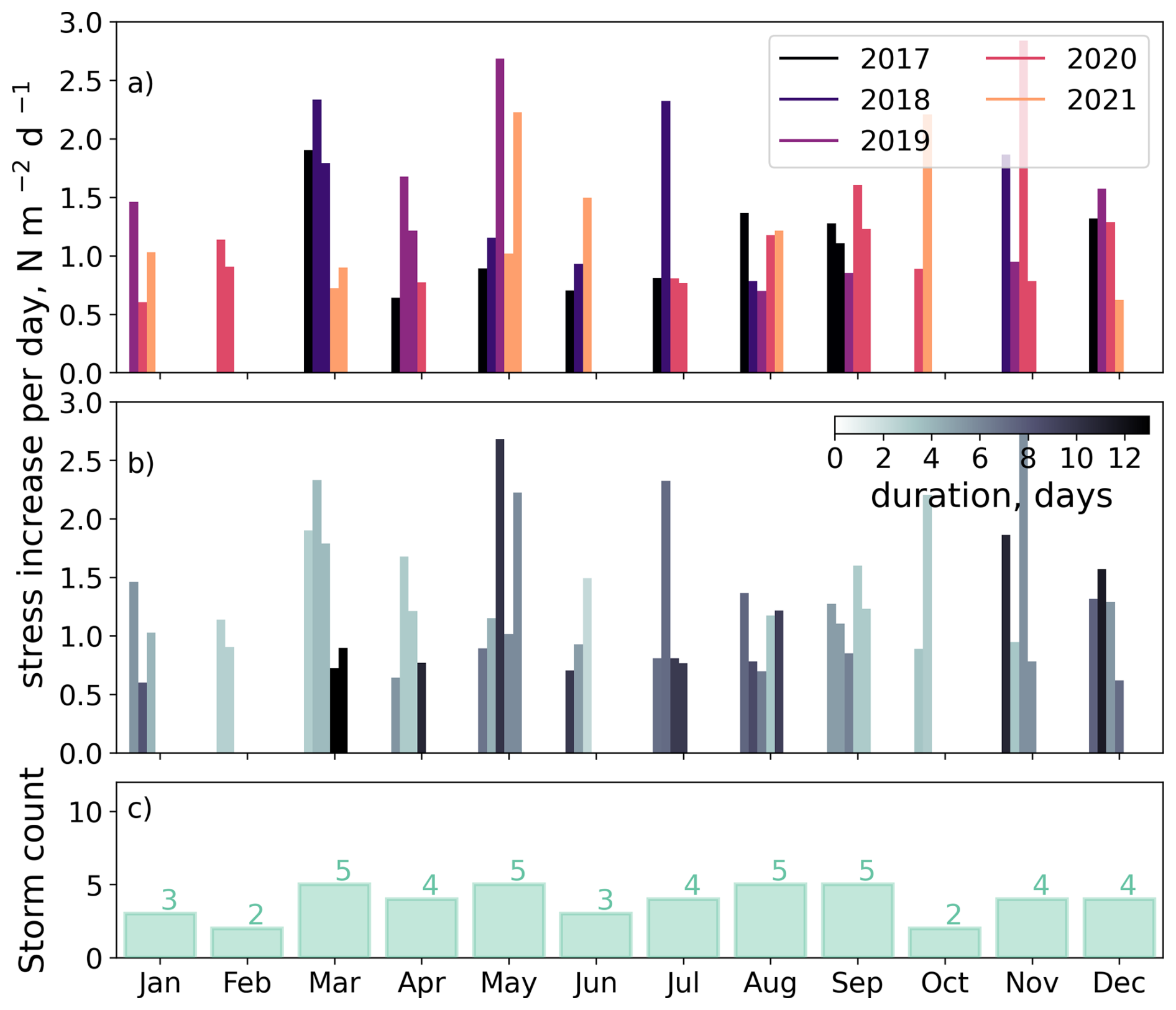
Figure 4 Storm statistics between January 2017 and December 2021. Panels (a) and (b) show the increase in ocean surface stress per day for the identified storm on the y-axis, with (a) year and (b) storm duration in color. Panel (c) shows the total number of storms per month.

2.5 Significant storm response

We define the “storm response” as the increase in current strength following a storm and quantify it as described below and illustrated in Fig. A1d. Prior to the analysis, the current records are low-pass filtered using a 4th order Butterworth filter with a cut-off at 40 h to remove shelf waves (Jensen et al., 2013) and tides.

For each storm, we determine the time (t=t₀) of maximum ocean surface stress, τ_max (sketch in Fig. A1d) and we identify the maximum current strength during a ten-day period spanning three days prior to and seven days after τ_max ($U_{max}(t_{\mathrm{0}}-\mathrm{3}\mathrm{d}:t_{\mathrm{0}}+\mathrm{7}\mathrm{d}))$. This maximum current is compared with the average current two days before the ten-day period ($U_{\mathrm{mean}}(t_{\mathrm{0}}-\mathrm{5}\mathrm{d}:t_{\mathrm{0}}-\mathrm{3}\mathrm{d})$). We define the difference between the two-day average and the maximum current as the “storm response” (U_response, Fig. A1d),

$$\begin{array}{}\text{(4)}& \begin{array}{rl}{U}_{\mathrm{response}}& =U_{max}(t_{\mathrm{0}}-\mathrm{3}\mathrm{d}:t_{\mathrm{0}}+\mathrm{7}\mathrm{d})\\ & -U_{\mathrm{mean}}(t_{\mathrm{0}}-\mathrm{5}\mathrm{d}:t_{\mathrm{0}}-\mathrm{3}\mathrm{d})\end{array}\end{array}$$

To assess whether a storm response is significant, i.e., whether the observed increase in current strength exceeds the background variability, we use a Monte-Carlo-like approach. We cannot conduct a traditional Monte-Carlo procedure due to the length of the storm events relative to the length of the time series – the overlap between sample periods would be too large to act as randomized tests. Instead, we estimate the current increase (U_response) during all 10 d-long, 50 % overlapping, storm-free windows (an example for M_slope1 is shown in Fig. A1c). If U_response during a storm is higher than the 90th percentile of U_response during the non-storm periods (vertical blue line in Fig. A1c), we consider the storm response significant. Each mooring has its own threshold for significance due to differences in the background variability (Table 2). The number of 10 d-long storm-free periods ranges from 96 to 215.

3 Results and discussion

We identify 38 strong ocean surface stress events that we classify as “storms” between February 2017 and February 2021 (Fig. 3). The storms are distributed relatively evenly throughout the four years, though the strongest and longest storms occur during spring and autumn (Fig. 4). All moorings consequently experience several storm events, and even the M_sill5 mooring, which has the shortest record length (20 months), experiences 13 storms (Fig. 3). We find that while many of the storms cause a significant response at the mooring locations, other storms do not (Fig. 3). Additionally, several storms cause a significant response at some of the mooring locations but not at all of them (Fig. 3).

3.1 Case study: Storm-driven circulation increase at all moorings

We present a case study of a particularly strong (${\mathit{\tau }}_{max}=\mathrm{1}$ N m⁻²) and long-lasting (10 days) storm event in March 2018 that affected all the mooring locations (Fig. 5a).

The storm response at M_slope1 and M_slope2 is associated with an increase of the ASC of roughly 15 cm s⁻¹, that lasts for four days and occurs directly after the maximum peak in ocean surface stress (Fig. 5b). At both M_sill1 on the eastern flank of the sill and M_ST in the Small Trough, the response is associated with a significant increased of the southward current a few days after the storm maximum, although the ocean current anomaly is shorter than at the slope (1–2 d, Fig. 5c). At M_sill5, the storm causes a significant increase in the outflow of DSW (Fig. 5d), although the high variability during the storm period at this mooring makes this less evident in Fig. 5d than at the other mooring locations. At M_CS2, along the eastern flank of Filchner Trough at 76° S, the southward storm response reaches 10 cm s⁻¹, and the maximum current occurs shortly after the maximum ocean stress (Fig. 5e).

This storm, which gives a clear current response all the way south at M_CS2, is caused by a large low-pressure system positioned over the southern Weddell Sea (Fig. 6a). The cyclonic circulation of the low-pressure system hugs the coastline, creating a patch of anomalously high along-coast wind stretching from roughly 30° W to 20° E (Fig. 6b). During the three days before and after τ_max, the high wind speed builds up and dies down without an evident along-coast propagation (not shown). The average sea ice concentration on the eastern continental shelf and upstream of the trough is lower than the sea ice climatology, and the sea ice movement is relatively high over the continental shelf break (Fig. 6c, d). This case study emphasizes the remote effect that upstream ocean surface stress conditions can have on the local Filchner Trough circulation, in agreement with, e.g., Daae et al. (2018) and Lauber et al. (2023).

3.2 Composite analysis: the mean storm response

Our case study suggests that a storm can cause both an enhanced ASC and enhanced currents far south along the flank of both Filchner Trough and the Small Trough. We, therefore, conduct a composite analysis of the mooring records using the identified storms to determine the mean storm response. For each mooring we make two composites: one for storms that give a significant storm response at the mooring and one for storms that do not.

Our results are sensitive to the choice of threshold for a significant storm response (held at the 90th percentile of current increase). If we lower the significance threshold from, e.g., the 90th to the 70th percentile, the percentage of storms that are considered to give a significant response at both slope-moorings (M_slope1 and M_slope2) increases from 34 % to 66 % (Fig. 3). However, we choose to keep our threshold at a conservative value to ensure that we focus on the strongest events with the most notable ocean responses.

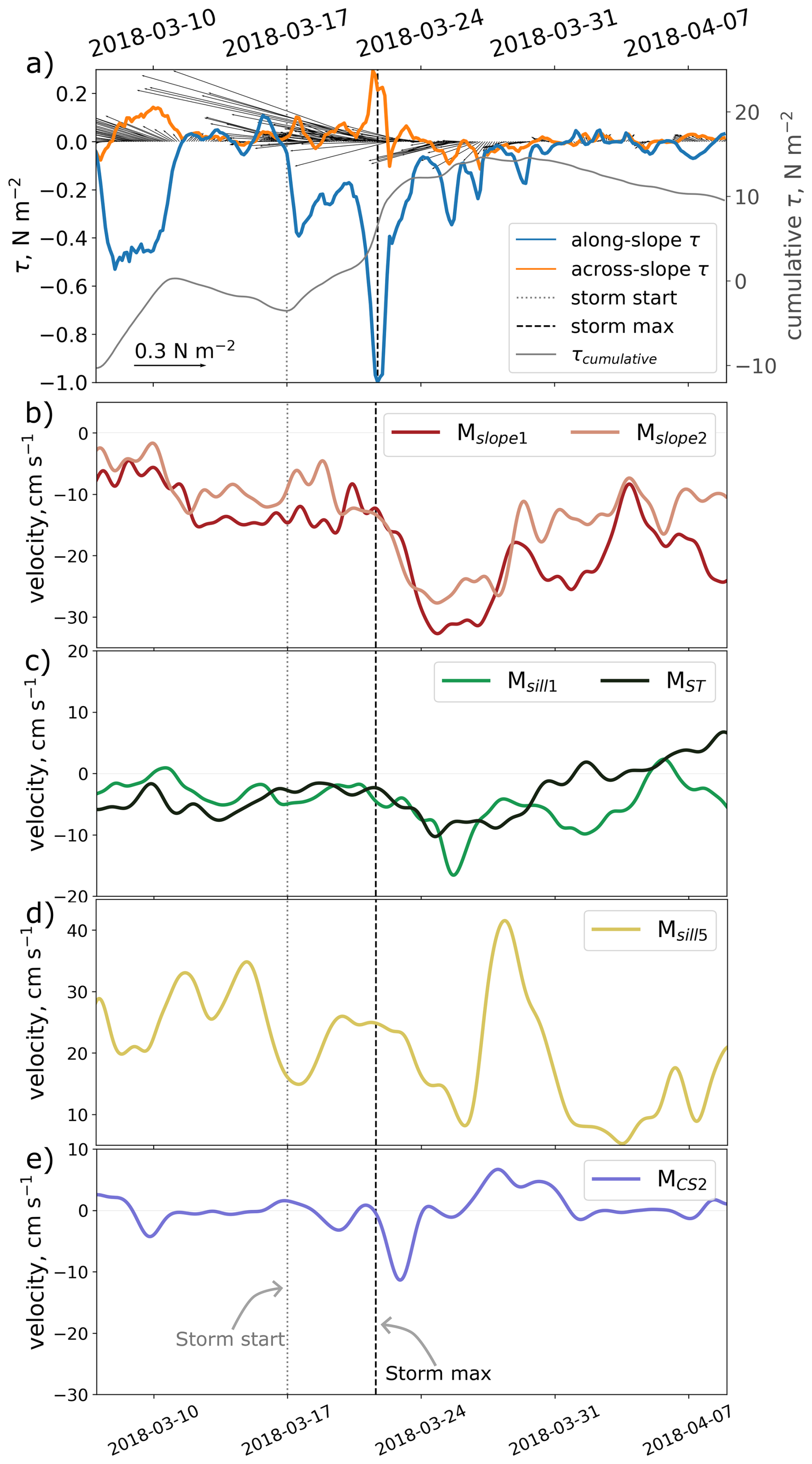
Figure 5 The response to the storm event that started on the 17 March 2018 (dotted, gray vertical line) and reached maximum ocean surface stress, τ_max, on the 22 March 2018 (dashed, black vertical line). Time series of (a) ocean surface stress (τ) averaged over the Upstream box (black sticks), the strength of the along-slope (blue) and cross-slope (orange) components, and the cumulative along-slope τ (gray, de-trended and 180 d high-pass-filtered). The along-flow current speed at (b) M_slope1 (red) and M_slope2 (pale red), (c) M_sill1 (green) and M_ST (gray), (d) M_sill5 (yellow), and (e) the current speed following the bathymetry at M_CS2 (purple). See Fig. 1 for mooring locations.

We expect the strongest storm responses at M_slope1 and M_slope2, since they are located over the slope and capture the acceleration of the ASC directly. Here, the mean current speed during the identified response-giving storms is 54 % higher than the mean current at M_slope1 and 50 % higher at M_slope2 (Table 2). Half the storms cause a significant increase in the along-flow current (average U_response of response-giving storms: $\sim -\mathrm{8}$ to −9 cm s⁻¹, Figs. 3, 7a, d, and Table 2).

The thermocline over the slope, represented by the −1.7 °C isotherm, is only weakly pushed down (on average ∼ 30 m at M_slope1 and ∼ 40 m at M_slope2 during the storms with a significant response at M_slope1 and M_slope2, not shown). This is substantially less than the high-frequency fluctuations in thermocline depth caused by shelf waves and tides (which are on the order of 100–200 m, Semper and Darelius, 2017; Jensen et al., 2013), and thus, depression of the thermocline caused by the storms does not substantially impede the access of warm water onto the continental shelf. The thermocline response to storm events is similar in summer and winter (28 and 33 m at M_slope1, respectively). Our results, therefore, do not support the hypothesis that the ASF may be protected from the wind by the fresh and warm surface layer during summer, as suggested by Daae et al. (2017) and Hattermann (2018).

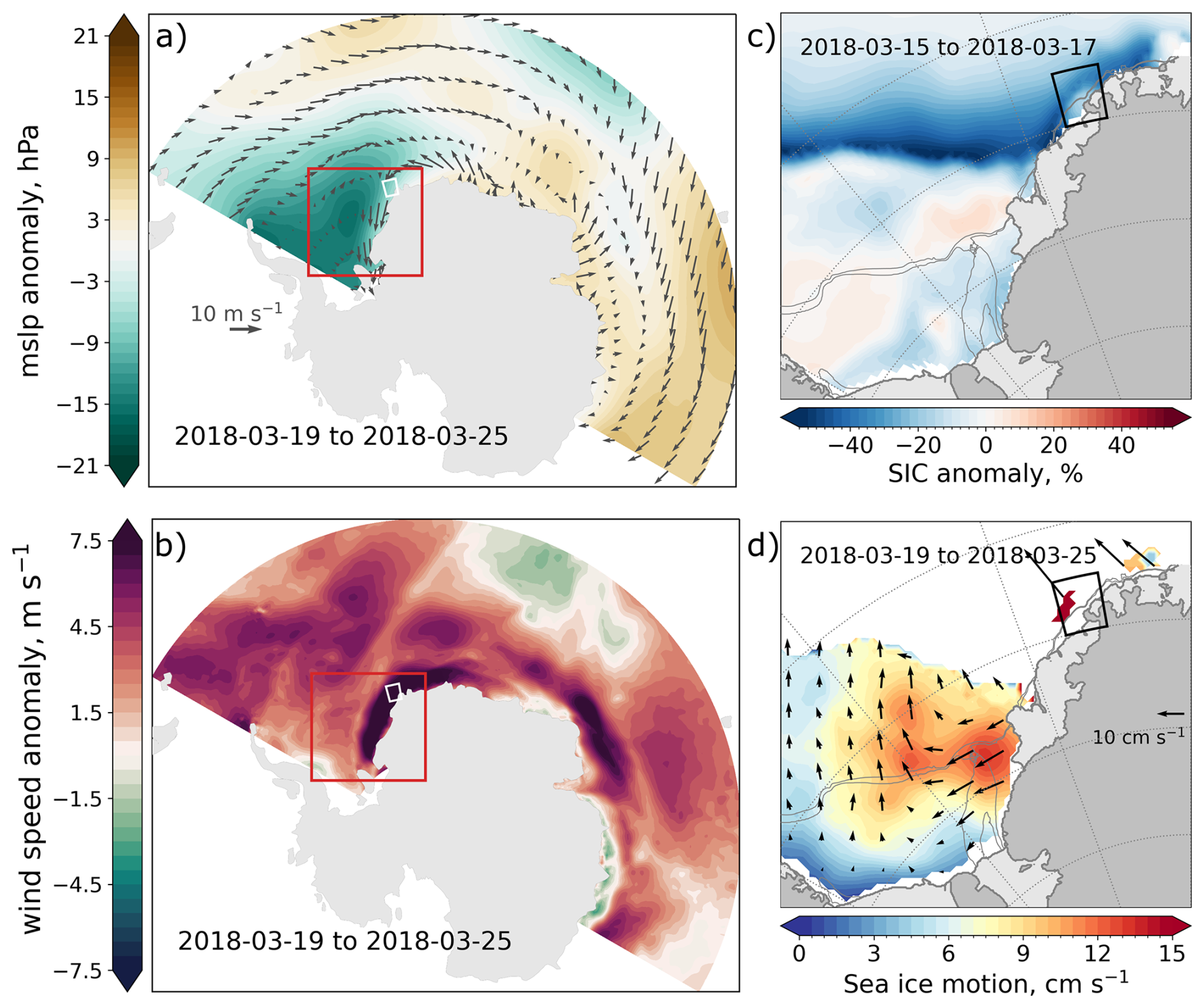
Figure 6 The atmospheric and sea ice conditions during the storm that started on the 17 March 2018 and reached maximum ocean surface stress, τ_max, on the 22 March. Anomalies of the (a) mean sea level pressure with 10 m wind velocity vectors and (b) absolute 10 m wind speed averaged ±3 d of τ_max relative to the average March field (1990–2023). (c) Sea ice concentration averaged over the two days before the storm starts relative to the climatology (past 30 years). (d) Sea ice velocity (Tschudi et al., 2020) averaged ±3 d of τ_max. White regions indicate missing data or areas without sea ice. In (a), (b), the Upstream box and the region shown in (c), (d) are indicated, and in (c), (d), the 1000 and 600 m isobaths are indicated by gray lines (Fretwell et al., 2013). Sea ice concentrations, pressure, and 10 m wind data are from ERA5 (Hersbach et al., 2023).

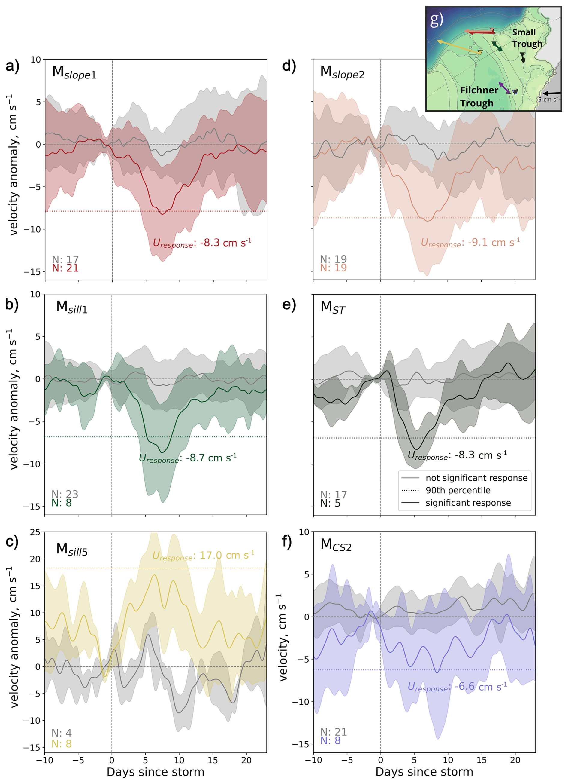
Figure 7 The composite average storm response at (a) M_slope1, (b) M_sill1, (c) M_sill5, (d) M_slope2, (e) M_ST, and (f) M_CS2. In each panel, the average response (line) and the standard deviation (area) to storms that give a significant response are shown in color, while the average current following storms that do not give a significant response is shown in gray. The legend in (e) is common for all panels. The threshold for significance (see Table 1, horizontal colored, dotted lines) and the number of events (N) included are indicated. Day zero is the start of the period used to estimate U_response, i.e., t₀−3 d (see Fig. A1). We only include the events where we have data for the 33 d shown in each panel. The map in the upper corner (g) shows the mooring locations and the mean current directions.

Both within the inflow across the Filchner sill and in the Small Trough (M_sill1 and M_ST) roughly 25 % of the storms cause a significant storm response (average response: −8.7 and −8.3 cm s⁻¹, Fig. 7b, e, Table 2). At M_sill1, all events with a significant response occur between December and June, i.e., from late spring to early winter (Fig. 3), although only 57 % of all the storms occur during these months (Fig. 4c). There is also a tendency for a seasonal signal at the slope moorings, where 70 % of the events that cause a significant storm response occur in this period.

Table 2 Overview of parameters from the composite analysis of storm response (U_response, Eq. 4) at the moorings. The % of response-giving storms is estimated relative to the storms occurring during each moorings record.

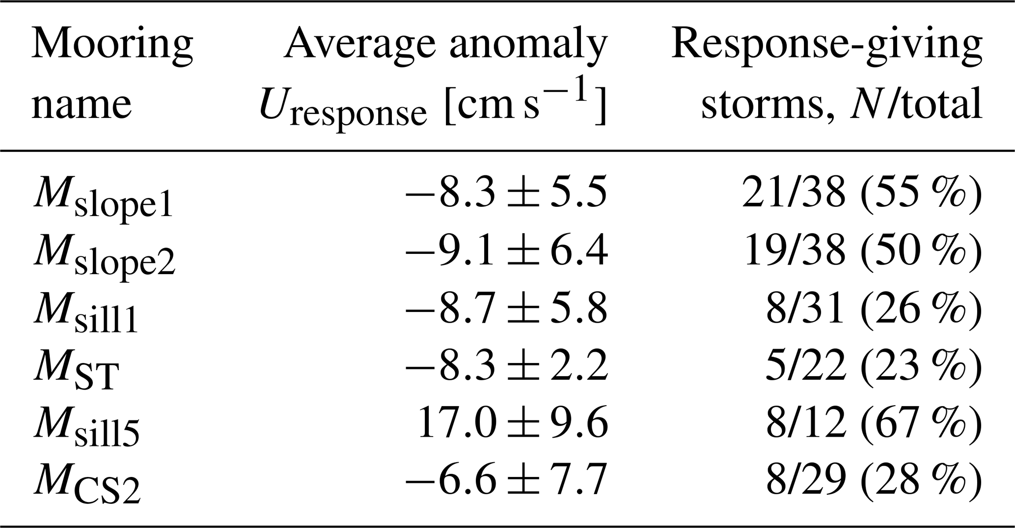
Within the observed ISW outflow, at the location of M_sill5, periods of strong along-slope wind co-vary with enhanced overflow on monthly time scales (Daae et al., 2018). Idealized numerical experiments (Dundas et al., 2024) also suggest that storms can adjust the SSH across a trough, thus connecting the southward inflow and the northward outflow. This is similar to the situation described by Morrison et al. (2020) and observed by Darelius et al. (2023a), where the downslope flow of DSW along a canyon or ridge causes an SSH anomaly that drives an upslope flow of WDW east of the corrugation. We therefore expect the storms to induce enhanced outflow (i.e., northward flow) at M_sill5 and this is confirmed by the observations (Fig. 7c, Table 2).

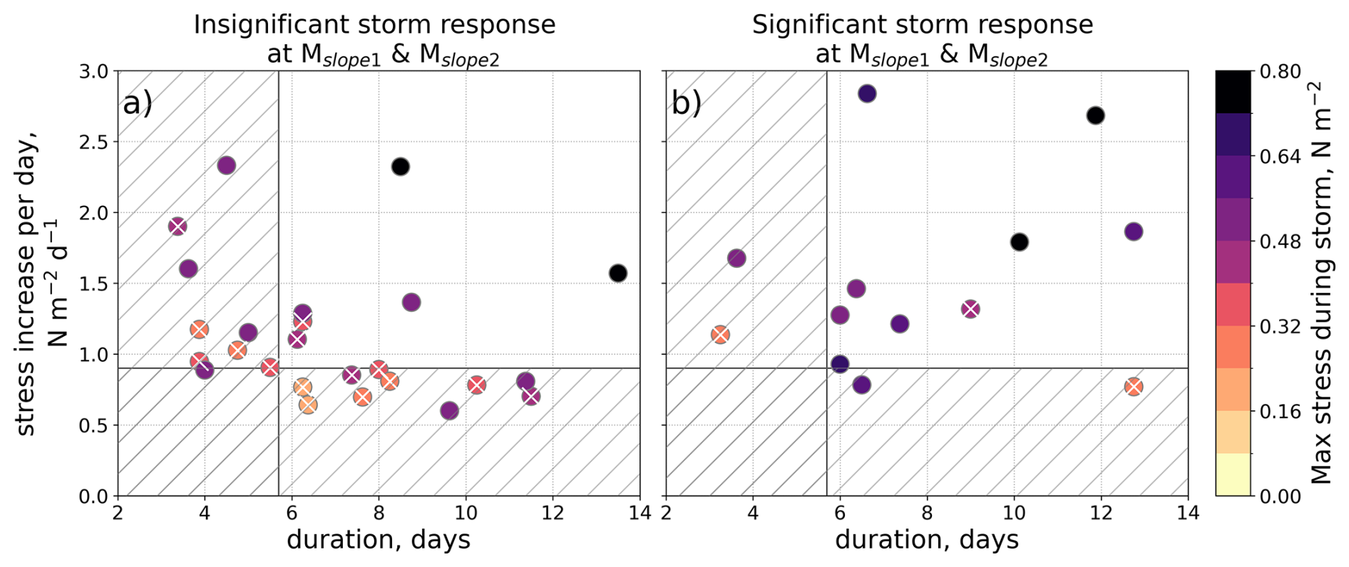
Figure 8 Scatter plots of storm duration and ocean surface stress increase per storm day, colored by the corresponding τ_max. The storms that do not induce a significant response at M_slope1 and M_slope2 are shown in panel (a), and those that do are shown in panel (b). The hatched area indicates a duration shorter than 5.7 d and/or a stress increase smaller than 0.9 N m⁻² d⁻¹. White crosses mark storms with ${\mathit{\tau }}_{max}<\mathrm{0.5}$ N m⁻².

Most of the strongest storm events (stress increase rate > 1.5 N m⁻² d⁻¹) occur between December and June (Fig. 4). Strong and long storm events are expected to cause the largest current response (Dundas et al., 2024), and thus, the seasonality in storm intensity (although weak) might contribute to the tendency of seasonality in storm response at M_sill1, and M_ST. The enhanced current during winter (Darelius et al., 2024a) could also cause a larger current pathway overshoot at the Filchner Trough opening (Daae et al., 2017), preventing the storm signal from propagating southward and reaching the mooring locations on the shelf, thus contributing to the tendency of fewer significant storm response events during winter.

At the southernmost mooring location, at M_CS2 along the eastern flank of Filchner Trough, 28 % of the storms cause a significant response (Fig. 3, average response: −6.6 cm s⁻¹ Fig. 7f). The fact that significant storm responses are recorded at this location highlights the potential for storms to increase the southward heat transport towards Filchner Ice Shelf. If warm water is present on the continental shelf during a response-giving storm, this warm water will likely be pushed southward as observed by Darelius et al. (2016). However, it will not necessarily reach the mooring during the storm event due to the relatively long background advection time scales (5–9 weeks) from the continental slope to 76° S (Steiger et al., 2024).

3.3 Which atmospheric conditions trigger a storm response?

The composite analysis of the mooring records shows that while some storms enhance the circulation, other storms do not. To investigate the atmospheric conditions that give a significant storm response we focus on the slope moorings (M_slope1 and M_slope2) since these records are the longest and since most of the storms that induce a response on the Filchner Sill and in the Small Trough also give a response on the slope (Fig. 3).

We find that an ASC response to a storm depends on the storm duration, the ocean surface stress increase during the storm, and the maximum stress (Fig. 8). Between 2017 and 2021, 70 % of storms that are (i) longer than 5.7 d, (ii) have a rate of stress increase larger than 0.9 N m⁻² d⁻¹, and (iii) have maximum stress higher than 0.5 N m⁻² over the Upstream box, give a significant storm response in the slope moorings.

Looking at large-scale atmospheric patterns, the low-pressure systems that give a response at M_slope1 and M_slope2, i.e., significantly enhance the ASC above the upper part of the continental slope, are deep (Fig. 9a). The average pressure at the center of the response-giving storms is 968 hPa. Both the wind speed and the sea ice movement are thus enhanced along the coast upstream of the study area (Fig. 9b, d). Prior to the storm events, the sea ice concentration is also, on average, low compared to the climatology when there is a response (Fig. 9c). In comparison to these conditions, the conditions during the storms that do not significantly enhance the ASC are less intense. The average pressure at the center of the storms without a response is 978 hPa, and the wind speeds and the sea ice movement are lower (Fig. 9e, f, h). The sea ice concentration is also more similar to the climatology (Fig. 9g).

Based on the composites and the case study (Fig. 5), we thus suggest that relatively low sea ice concentration, high sea ice mobility, and strong wind along the coast upstream of the study area are conditions that favor a significant storm response. This is also expected, as these conditions lead to an efficient momentum transfer from the atmosphere into the ocean, enhanced Ekman convergence, and an increased cross-slope SSH-gradient that drives a barotropic response in the ASC.

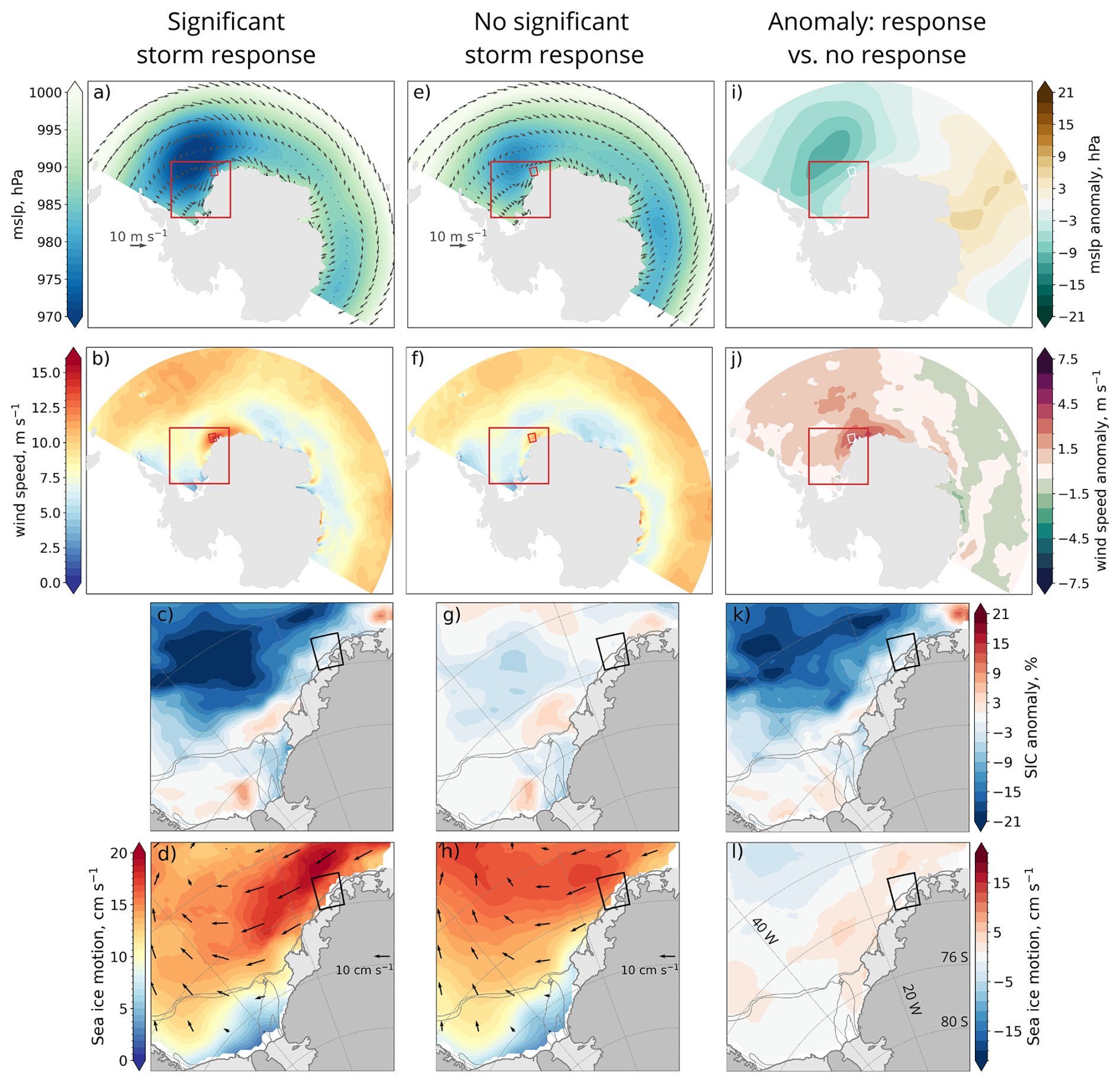
Figure 9 Composite mean atmospheric fields during storms (a–d) with and (e–h) without a significant storm response at M_slope1 and M_slope2. The difference between the fields during storms with and without a response is shown in (i)–(l). The first row shows the mean sea level pressure (color) and the mean 10 m wind (gray arrows) ±3 d of τ_max. The second row shows the wind speed in color and is otherwise equal to row one. The third row shows the mean sea ice concentration anomaly (with seasonal climatology removed) in a two-day window ending when the storm begins. The fourth row shows the speed of the sea ice motion (color) and its velocity (black arrows) ±3 d of τ_max. White regions along the coast indicate missing data or areas without sea ice.

3.4 A shift in mid-2019

An apparent change in the storm response occurs during 2019, which is most prominent at M_CS2: Before July 2019, only one storm event caused a significant response at this location, while after July 2019, 40 % of the storms caused a significant response (Fig. 3). For the slope moorings, there is a similar but opposite tendency. Here, there are fewer significant storm response events after July 2019 (Fig. 3). While we cannot rule out that this is a coincidence, these results indicate that (i) the potential for a significant storm response depends on conditions that vary interannually and (ii) a storm response at M_CS2 is not necessarily propagating from M_slope1 and M_slope2 southward along Filchner Trough. The latter is contrary to results from the idealized numerical simulations in Dundas et al. (2024), where the ASC and the circulation on the shelf east of Filchner Trough were tightly connected. We suggest that the complex bathymetry – and potentially the interplay between the Antarctic Coastal Current and the ASC – are important factors that explain the differences between the results of the idealized model and the observations presented here.

Interannual variability in the sensitivity to wind forcing on monthly time scales was also observed in the Antarctic Coastal Current (M_CC, mooring location shown in Fig. 1) and on the sill of Filchner Trough (15 d low-pass-filtered, Daae et al., 2018). This variability was associated with shifts in the average wind direction and its strength along the coast upstream of Filchner Trough: When the wind had a northwestward component and the wind speed was low, the significant correlation, estimated between the wind and the current, weakened. We do not observe a substantial change in the direction of the mean ocean surface stress before and after mid-2019 (not shown), and while there is a reduction in the variability and average strength of the zonal stress, these changes are minor (Fig. B1e). There is neither an apparent change in the strength nor the duration of the storms (Figs. 4 and 3).

We do, however, identify several changes in the background circulation and hydrography on the shelf during 2019 (Fig. B1). After July 2019 (i) the current at M_CS2 veers eastward (Fig. B1f), (ii) the correlation, estimated following Sciremammano (1979), between the along-coast wind and the along-isobath current at M_CS2 changes sign (Fig. B1a), (iii) ISW starts to dominate the winter hydrography at M_CS2 and is associated with increased variability in the current (Fig. B1b). Additionally, we note that (iv) a transition from “Berkner mode” to “Ronne mode” occurred in mid-2018 (Hattermann et al., 2021; Janout et al., 2021), (v) at the shelf break the warmest water is anomalously warm and the seasonal cycle is disrupted after mid-2019 (Darelius et al., 2023b) and that, (vi) the summertime sea ice concentration increases in 2019 (Steiger et al., 2024).

It is beyond the scope of the present study to investigate the relationship between these changes and the apparent shift in the regional storm response. We note, however, that changes in the summer sea ice cover are likely to play a role, as it agrees with the results of the composite analysis that low sea ice concentration favors significant storm responses in the ASC. A more detailed presentation and discussion of the changes occurring in 2019 is found in Appendix B.

4 Conclusions

We analyze a network of moorings and confirm that storms can enhance the circulation on the southeastern Weddell Sea continental shelf. These events do not have a systematic significant ocean current response but when they do, they clearly strengthen the westward Antarctic Slope Current (ASC), the dense outflow from Filchner Trough, the southward flow along the eastern flank of Filchner Trough, and the inflow through the Small Trough. Our findings provide observational evidence that storms can enhance the southward transport of warm water towards the Filchner Ice front, as suggested by Darelius et al. (2016) and by the numerical experiments of Dundas et al. (2024). The duration of a storm, the total cumulated ocean surface stress during the event, and the maximum stress, will, to a large extent, determine whether a storm event enhances the ASC: 70 % of the observed storms that are longer than 5.7 days, have a larger stress increase than 0.9 N m⁻² d⁻¹, and ${\mathit{\tau }}_{max}>\mathrm{0.5}$ N m⁻², give a significant increase in the ASC.

The interannual variability in the storm response – notably the apparent shift in 2019 that we are unable to explain – highlights the importance of ambient conditions in determining the response of the ASC and the currents on the continental shelf to wind forcing. It also points to a knowledge gap that needs to be addressed if we are to predict how the system evolves in a future of climate change.

Longer observational time series from the region, in combination with designated experiments in a regional model setup, would help us to further understand the observed variability in storm response. A regional model could also provide estimates of the storm-driven heat transport across the shelf and its importance relative to the heat transport driven by the background flow. The present study, however, provides evidence that storms along the coast upstream of Filchner Trough can enhance the circulation on the shelf, potentially allowing heat to reach the ice front before it is lost to the atmosphere through wintertime convection.

Appendix A: Supporting figures

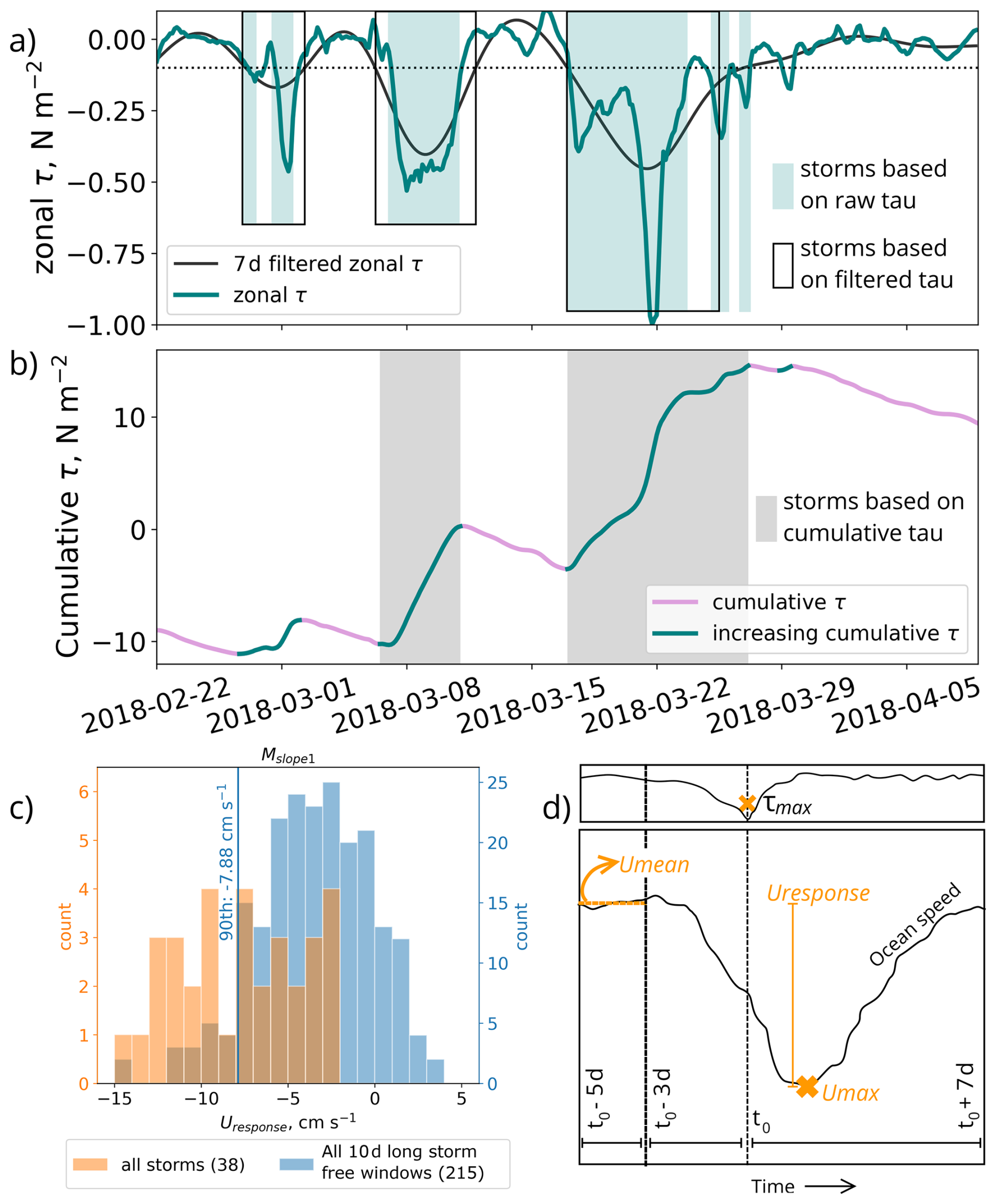
Figure A1 (a, b) Example of the storm detection algorithm described in Sect. 2.3. Time series of (a) eastward ocean surface stress and (b) the cumulative westward ocean surface stress. Identified storm periods are indicated based on (a) the raw ocean surface stress (blue shading) and lowpass filtered ocean surface stress (black boxes) and (b) based on cumulative ocean surface stress (gray shading), which we use throughout our analysis. (c, d) Illustrate the procedures used to determine significance and to identify U_response as described in Sect. 2.5. (c) Histogram of U_response (orange) and the current increase during all 10 d long storm-free windows (blue) at M_slope1. The 90th percentile, which is used to determine significance, is indicated (blue line). (d) A sketch of the procedure used to identify U_response, indicating the definition of τ_max in the upper sub-panel and U_mean, U_max, and U_response in the lower sub-panel.

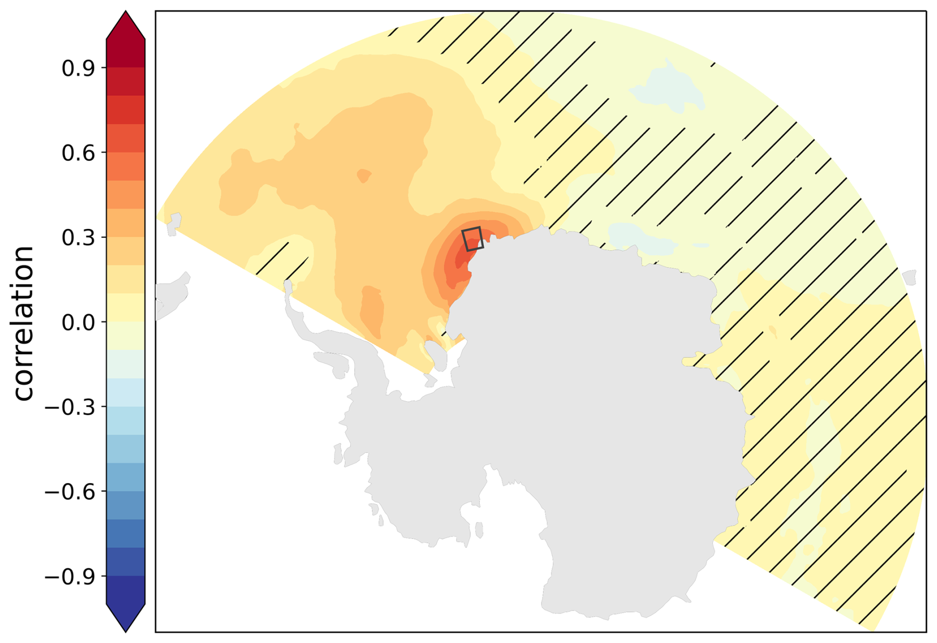
Figure A2 Correlation map of the average wind speed in the Upstream box (black rectangle) vs. the overall wind field during the observation period (2017–2021). Hatched regions indicate insignificant correlation at the 0.95 significance level, following Sciremammano (1979).

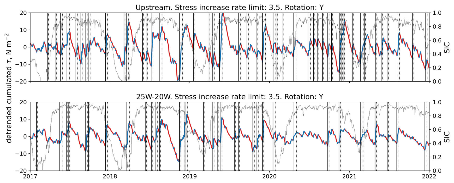
Figure A3 Time series of cumulative and detrended ocean surface stress over the upstream box (upper panel) and a region further west (25 to 20° W) to indicate the difference in storm identification. Solid black lines indicate storm start and dashed lines are the storm end. The blue parts of the curve highlight increasing cumulative ocean surface stress while the red parts are decreasing.

Appendix B: Changes during 2019 and possible connections to oceanic storm response

The consistent eastward direction of the current at M_CS2 from 2019 and onwards (Fig. B1f) is in stark contrast to the current at this location from 2014 to 2016: then, the current had a strong seasonal cycle with a southwestward direction during the warm season and west or northward during the cold season (Ryan et al., 2017). We speculate that the interannual variability in storm response may be related to changes in background circulation at the location. This could be driven by variable interaction between the southward current along the eastern flank of Filchner Trough, the inflow through the Small Trough, and the Coastal Current as they all interact on the narrow continental shelf east of Filchner Trough at roughly 76° S. The complex bathymetry in the region of M_CS2 might thus hinder the southward signal from propagating neatly southward as it does in the model setup with idealized geometry (Dundas et al., 2024).

Since the 2019 shift is not only locally present at 76° S but also appears in the storm response on the slope, it is possible that properties of the Antarctic Coastal Current might affect the shift. Daae et al. (2018) observe a shift in the correlation between wind and the currents (on monthly time scales) at moorings from the Filchner Sill and the Coastal Current (M_CC) between 2003 and 2004 (locations indicated in Fig. 1). The Coastal Current (on the shelf) had the strongest correlation with the wind in 2003, while the outflow at the sill showed the highest correlation in 2004 (Daae et al., 2018). This shift is hence similar to the shift in storm response we observed in 2019: the storm response on the shelf increases when the storm response on the slope decreases. One possible explanation could be that the storm-enhanced signal under certain conditions propagates mainly along the shelf break, causing a strong signal at the slope moorings, and in other not yet identified conditions, mainly propagates along the coast, causing a strong signal at the M_CS2 mooring. In such a scenario, we would, however, also expect a stronger storm-response at a mooring located just east of M_CS2 from mid-2019 onwards, but this is not the case (not shown). In mid-2018, the circulation under the northern section of Filchner Ice Shelf changed from “Berkner mode” to “Ronne mode” (Hattermann et al., 2021; Janout et al., 2021). This means that the source waters of the ISW observed in the Filchner cavity originated from the Ronne Trough after 2018 rather than from the Berkner Shelf. We considered the possibility that the mid-2019 shift in storm response at the M_CS2 location could be a delayed response (roughly one year lag) to this large-scale shift in circulation and hydrography. However, at M_CS3, which captures the northward-flowing ISW leaving the cavity, indications of the change from Berkner to Ronne mode appear in 2018. Following the start of 2019, Ronne-sourced ISW is already consistently present at 76° S and the current has veered eastward (Fig. B1c, f). Due to this offset in timing between the shift in hydrography and circulation following the transition from Berkner to Ronne mode and the shift in storm response along the continental slope (M_slope1 and M_slope2) and in Filchner Trough (M_CS2), we are hesitant to suggest a direct link between the events. What causes the interannual shift in storm response in the southeastern Weddell Sea thus remains an open question.

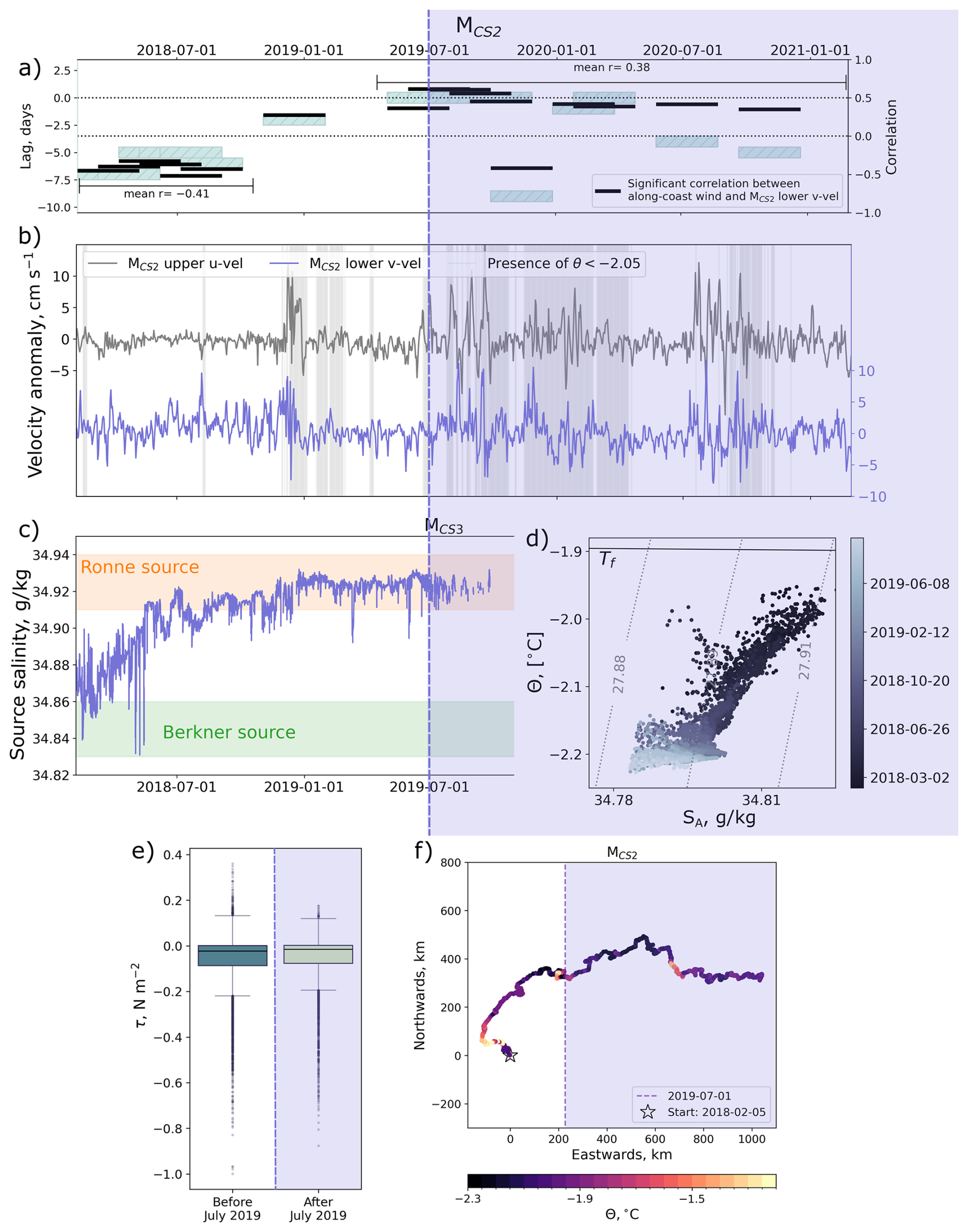
Figure B1 Indications of a shift around 2019 in the southeastern Weddell Sea shelf region. Panels (a)–(c) have a shared x-axis, the purple background indicates the period after 1 July 2019. (a) Time series from M_CS2 of 90 d long, 33 % overlapping windows of significant correlation (0.95 significance level, black bars) and lag (blue bars) between the along-coast wind and the southward bottom current, following Sciremammano (1979) (24 h–30 d bandpass filtered. Positive correlation: roughly south-westward wind corresponds to current toward Filchner Ice Shelf). (b) Current anomalies at M_CS2; eastward component at the upper sensor (gray) and the northward component at the lower sensor (purple) with gray shading when water colder than $\mathit{\theta }=-\mathrm{2.05}$ °C is present. (c) The estimated ISW source water salinity at M_CS3 with approximate ranges of Berkner (green shading) and Ronne (orange shading) mode source waters (Hattermann et al., 2021). (d) ΘS_A-diagram from M_CS3 colored by time. For clarity, we have omitted observations with σ<27.885 kg m⁻³ in panels (c) and (d). (e) Box plots of the along-slope ocean surface stress before (blue) and after (green) July 2019. (f) Progressive vector diagram of the current at the bottom sensor of M_CS2 colored by temperature. The temperature is based on the average absolute salinity (at the nearest sensor level) because the salinity sensor stopped recording in early 2020. The start of the time series (star) and the 1 July 2019 (dashed line) are indicated.

Appendix C: Source salinity estimates

To estimate the arrival of the shift from Berkner to Ronne mode described by Hattermann et al. (2021) and Janout et al. (2021), we estimate the source salinity of the waters whose temperature and salinity are measured at M_CS3 by identifying the intersection between the Gade line (Gade, 1979) and the surface freezing point in ΘS_A space (illustrated in Fig. C1). Solving the linear relationship given by Wåhlin et al. (2010) for the source salinity, S₀, gives

$$\begin{array}{}\text{(C1)}& S_{\mathrm{0}}=S\left[\mathrm{1}+{\displaystyle \frac{c_p}{L_{\mathrm{f}}}}(T_{\mathrm{0}}-T)\right],\end{array}$$

where c_p=4186 J kg⁻¹ K⁻¹ is the specific heat capacity of sea water and $L_{\mathrm{f}}=\mathrm{3.34}\times {\mathrm{10}}^{\mathrm{5}}$ J kg⁻¹ is the latent heat of fusion (e.g., Hattermann et al., 2021). By first estimating the surface freezing temperature, T₀, at the recorded salinity, S, and then using Eq. (C1) to estimate the corresponding source salinity, S₀, we obtain an initial estimate of where the salinity-dependent surface freezing point intersects with the Gade line. The calculation is repeated once, replacing S by S₀ to find a new T₀ and S₀ (Fig. C1).

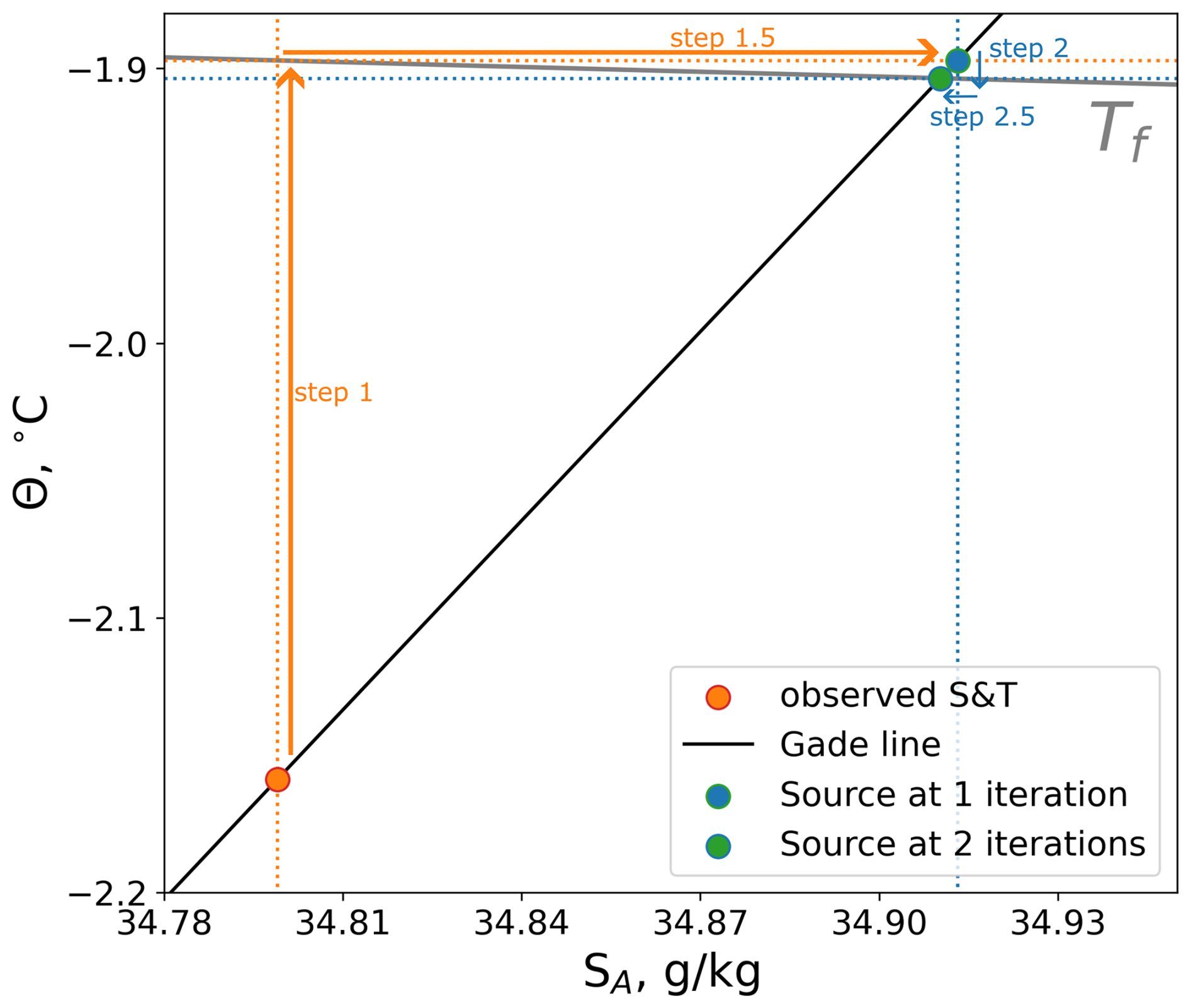
Figure C1 Illustration of the method to estimate source salinity following Eq. (C1). The desired value is the temperature and salinity at the intersection between the relevant Gade line (black line) and the salinity-dependent freezing point (gray line). The process is as follows: given an observed temperature and salinity pair (orange dot), the freezing point is estimated (step 1). Then, the salinity at this temperature of the Gade line is estimated (step 1.5). This completes iteration 1 and the first approximation of the source temperature and salinity (blue dot). Completing one more iteration (steps 2 and 2.5) gives a good approximation of the source water properties (green dot).