Flow structure and mixing near a small river plume front: Winyah Bay, SC, USA

This study presents Eulerian data from Winyah Bay, SC, USA collected during the passage of a tidal plume. The data captured the evolution and structure of the plume and include high-resolution velocity and temperature time series, supplemented by temperature – salinity profiles from a MicroCTD profiler. The observations identified a pre-existing plume extending to 4 m, with a water density of 1023.6 kg m⁻³, laying above denser ambient waters. Upon arrival, the newly discharged tidal plume introduced a fresher layer (1020.7 kg m⁻³) extending to 2.6 m, gradually thinning due to radial spreading. The plume's frontal propagation measured at 0.36 m s⁻¹ with a calculated Froude number of 1.32, indicating gravity current dynamics. In the across-front direction a return flow developed under the plume that extended throughout the water column, resembling an estuarine-like circulation pattern. Mixing processes were examined using the available overturn potential energy (AOPE) in the water column as described in Smith (2020). The analysis showed that near the bed, bottom boundary layer turbulence is the main mixing mechanism both before and after the passage of the front. In the surface layer, before the arrival of the front, mixing is driven by wind-induced shear and overturning. Within the gravity current, despite the high turbulent kinetic energy dissipation rates in certain regions, shear-induced mixing was minimal. These findings were reflected in the density diffusivity estimates near the surface that varied from 10⁻⁶ m² s⁻¹ prior to the arrival of the front, increasing to 10⁻⁵ m² s⁻¹ very near the front and diminishing to 10⁻¹⁰ m² s⁻¹ within the plume despite the high velocity shear observed there. The limited mixing within the plume despite the high shear observed can be explained using the concept of a layer-interface structure, where layers of high turbulence and low stratification alternate with regions of low turbulence and higher stratification. Although not resolved by these observations, this structure has been observed in numerical simulations of mixing. The development of the counter-flow under the plume suggests that tide and/or wind induced straining may play an important role in enhancing stratification in plumes like the one studied here.

1 Introduction

Freshwater tidal plumes are common features in coastal environments, where rivers discharge nutrient-rich freshwater into saltier ocean waters. A plume discharged during ebb tide behaves like a jet outflow as it enters the coastal ocean. In the absence of high winds and strong coastal currents it transitions into a buoyancy-driven surface current that expands under the action of gravity (i.e., gravity wave). Further offshore, and assuming there are no constraints on the flow, the plume will turn until it achieves geostrophic balance and will propagate as a Kelvin wave (Münchow and Garvine, 1993). Under realistic conditions, the geometry, structure, and dispersion paths of freshwater plumes depend on wind forcing, river discharge, coastal circulation (including tides), and bathymetry (Horner-Devine et al., 2015). Moderate upwelling-favorable winds drive the plume offshore, causing it to thin and stretch into filament-like shapes that can extend tens of kilometers (Li et al., 2003; Yankovsky et al., 2022). Conversely, under downwelling conditions, the plume is compressed against the coast, deepening as it is driven parallel to the shoreline (Fong and Geyer, 2002). During their evolution, tidal plumes exhibit distinct flow structures that resemble those found in gravity currents created in the laboratory by Britter and Simpson (1978). This was confirmed by Imberger (1983) and Luketina and Imberger (1987) who used field observations to develop a conceptual model showing the similarities between gravity currents and tidal plumes.

In the absence of strong wind forcing, radial spreading plays a significant role in mixing and plume evolution. Spreading stretches the plume horizontally, leading to thinning and increased velocity, which intensifies shear at the base of the plume. This shear drives mixing, which incorporates denser ambient water into the plume through entrainment. The density increase due to entrainment deepens the plume and reduces its buoyancy, which may subsequently decrease its lateral spreading rate and overall velocity as it transitions to subcritical flow (Hetland, 2010; MacDonald et al., 2007). Usually, the base of the plume experiences stratified-shear instabilities at the plume/ambient water interface, which may cause mixing between the two water bodies (Kilcher et al., 2012, MacDonald et al., 2007). The frontal region is the most energetic as it forms a convergence zone that extends several meters into the water column. The mixing and turbulence are intense (O'Donnell et al., 2008) and TKE dissipation rates are of the order of 10⁻⁴ to 10⁻³ m⁻² s⁻¹ diminishing exponentially to 10⁻⁷–10⁻⁶ behind the front (Orton and Jay, 2005; O'Donnell et al., 2008; Horner-Devine et al., 2013; Delatolas et al., 2023). Recently, Spicer et al. (2021) argued that bottom generated tidal mixing can also be important, especially under the influence of large tidal currents, as is the case for the Connecticut River discharging into Long Island Sound. Using a numerical model, they demonstrated that frontal mixing contributed only 10 % to the total mixing in that system, with the remaining 90 % being a balance between interfacial and tidal mixing, depending on tidal strength and river buoyancy input. Using a more realistic plume model, Whitney et al. (2024) showed that although tidal mixing in the Connecticut River plume is important, interfacial mixing is the largest contributor. Although both shear and convection have been recognized as potential mixing drivers in the ocean (Ivey et al., 2020), traditionally, plume studies have focused mainly on the effect of shear on mixing the water column. Numerical modeling work has also identified tidal straining (de Boer et al., 2006, 2008) as a mechanism that may enhance stratification in the coastal ocean even under high shear conditions, particularly during ebb and/or neap tidal phases. During ebb tide, freshwater advection rates may be increased, strengthening vertical density gradients, and during neap tide, shear may be reduced as tidal amplitudes decrease (Simpson et al., 1990; Souza and Simpson, 1996). However, while this phenomenon has been well-studied in estuaries, few observational studies have assessed its effect on river plumes, and those have focused more on effects of the spring-neap cycle (i.e., Rijnsburger et al., 2018).

To date, our improved understanding of coastal circulation is guided primarily by numerical modeling exercises. Such numerical experiments rely on existing parameterizations of turbulence and mixing to describe density diffusivity (K_ρ), a parameter that defines the rate at which fresh water is mixing with the ambient higher salinity water. It is usually expressed as:

$$\begin{array}{}\text{(1)}& K_{\mathit{\rho }}=\mathrm{\Gamma }{\mathit{\epsilon }}_{\mathit{\kappa }}/N^{\mathrm{2}}\end{array}$$

where ε_k is the turbulent kinetic energy (TKE) dissipation rate, N is the buoyancy frequency ($N^{\mathrm{2}}=-g/{\mathit{\rho }}_o\partial \mathit{\rho }\left(z\right)/\partial z$, where g is gravitational acceleration, and ρ is water density with the subscript o denoting ambient salty water) and Γ is the mixing efficiency parameter defined as the ratio of the dissipation rate (ε_p) of turbulent potential energy (TPE) to ε_k (Smith, 2020):

$$\begin{array}{}\text{(2)}& \mathrm{\Gamma }={\mathit{\epsilon }}_p/{\mathit{\epsilon }}_k\end{array}$$

The parameter Γ represents the amount of turbulent kinetic energy expended to mix the water column in coastal stratified systems, and is used widely to model mixing and estimate buoyancy fluxes in quasi-steady shear flows. The stratified state of the water column is characterized by its turbulent potential energy that represents the energy associated with the potential difference between the averaged and fluctuating states of the water particles. Following Osborn (1980), Γ is commonly parameterized using the flux Richardson number (Ri_f) so that$\mathrm{\Gamma }=R{i}_{\mathrm{f}}/\left(\mathrm{1}-R{i}_{\mathrm{f}}\right)$; in the absence of a robust expression for Ri_f (e.g., Mater and Venayagamoorthy, 2014), it is usually assumed that Γ≈ 0.22 (Peters, 1999; Kay and Jay, 2003; MacDonald and Geyer, 2004; Osborn, 1980). However, Scotti (2015) showed that for isotropic overturn Γ≈2. Burchard and Hofmeister (2008) in their work on mixing and stratification in estuaries and coastal seas (applying Simpson's (1981) concept of potential energy anomaly ϕ) used a bulk mixing efficiency Γ=0.04, while Simpson et al. (1990) used a value of 0.003. Lozovatsky and Fernando (2013), motivated by the variability of Γ and Ri_f estimates in the literature, re-examined mixing processes to conclude that mixing efficiency depends on both the gradient Richardson number (Ri_g) and the buoyancy Reynolds number (Re_b). They argued that a constant mixing efficiency value can be used only for a limited range of Ri_g and Re_b values representing conditions where turbulence is internally generated, stationary and homogeneous. More recently, Caulfield (2021) highlighted the complexity of mixing processes, and the different scales involved. He emphasized the tendency for layer-interface structures to develop, where a small vertical range of rapid density change separates relatively well-mixed regions. Within these strongly stratified structures, turbulence is generally inhibited, but small regions of weaker density gradients can generate strong turbulence. Given the broad range of values presented in the literature, and the limited comparisons between real-world measurements and parameterizations (see reviews by Gregg et al., 2018 and Caulfield, 2021), there is a need to provide additional data sets to better constrain these parameterizations.

The objectives of this study are three-fold: (i) to present high quality experimental data of flow structure, stratification and turbulence from a relatively new site in the SE US and as such to enrich the database on tidal plume dynamics data available to the community; (ii) to examine how plumes interact with the ambient coastal ocean and determine the modification, if any, of the ambient water flow structure; and (iii) to evaluate mixing mechanisms and the relation of TKE dissipation rates to density diffusivity within a gravity plume.

Our study engages with the broader theoretical and observational efforts to understand circulation and mixing in buoyant, stratified flows, building off prior work (e.g., Marmorino and Trump, 2000, O'Donnell et al., 2008, Spicer et al., 2022). We utilize advanced methodologies to investigate full water column flow and density structure in the vicinity of the Winyah Bay, SC (USA) tidal plume front, under light upwelling wind conditions. High-resolution Eulerian time series of flow, temperature, and turbulence structure, extending close to the sea surface, are analyzed alongside individual temperature-salinity (T-S) profiles. Turbulent kinetic and potential energy dissipation rates (ϵ) are estimated using a combination of acoustic Doppler current profiler (ADCP) based techniques (Zeiden et al., 2023) and Thorpe sorting approaches (Smith, 2020). These methods allow for precise characterization of turbulent signals, mixing processes, and hydrographic characteristics (temperature, salinity, and density) across the plume front. By integrating these state-of-the-art approaches, this study provides details on tidal plume kinematics and assesses mixing efficiencies with unprecedented detail.

2 Experimental Setup

2.1 Data Collection

Data collection took place outside the mouth of Winyah Bay, an estuary located in South Carolina, USA. It is 29 km long, extends over an area of 157 km² and receives water from a drainage area of 47 060 km². It is a microtidal system, subjected to semidiurnal tides with a mean tidal range of 1.4 m at the mouth which at its narrowest point is 1.2 km wide and ∼ 8.2 m deep (Kim and Voulgaris, 2005). The data presented here were collected as part of a larger synoptic survey of the Winyah Bay plume that occurred on board the R/V Savannah during the period 12 to 15 April 2023. This includes time series of velocity and temperature profiles, accompanied by distinct CTD and turbulence structure profiles collected at a single site (TS2) located some 10 km off the mouth of the estuary (Fig. 1). The mean water depth was 11.5 m, and the bathymetry is relatively smooth (see Fig. 1a). The site was selected with the aim of capturing the propagation of a newly discharged tidal plume as it entered the coastal ocean.

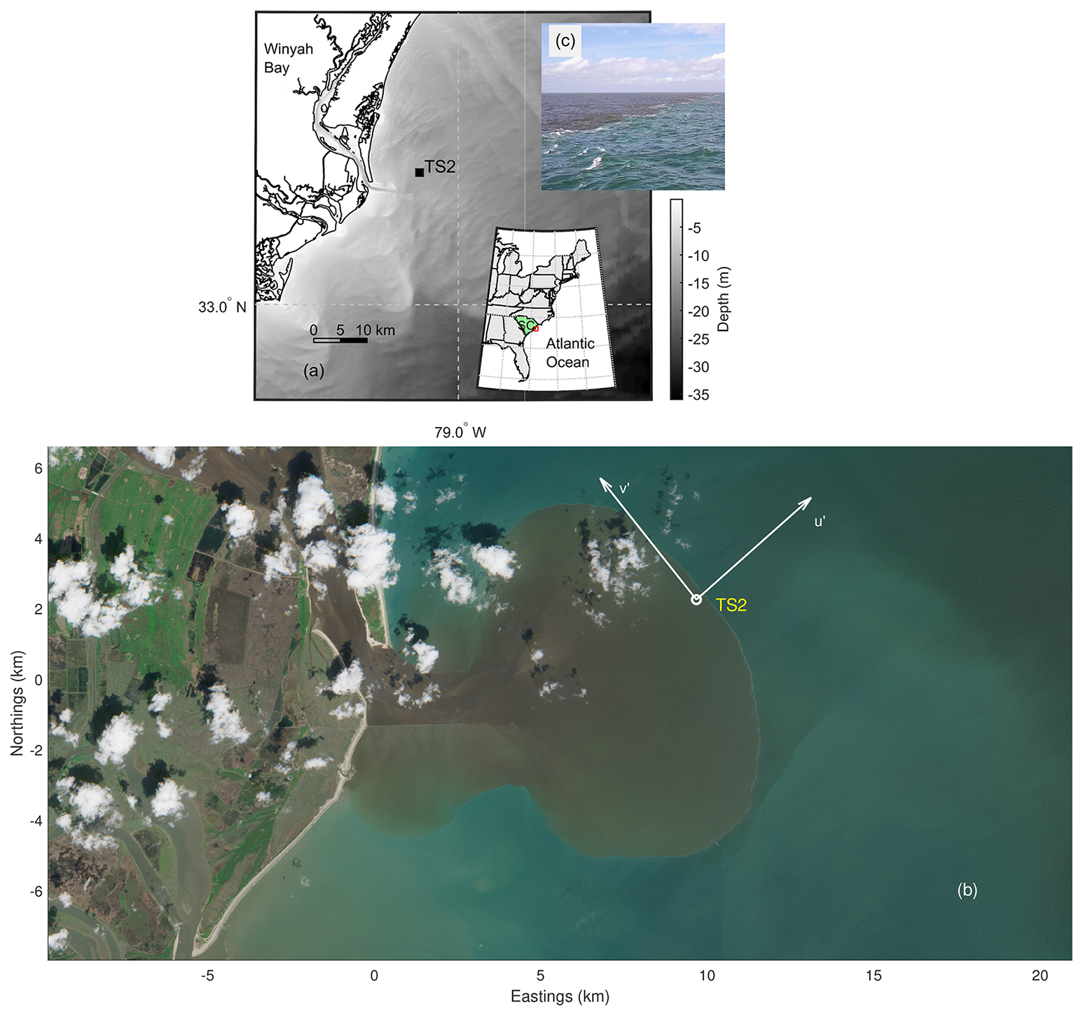
Figure 1 (a) Location of time series data collection (station TS2) off the coast of South Carolina, USA. (b) Sentinel L2 satellite image (modified Copernicus Sentinel data 2023 processed by Sentinel Hub) of a plume exiting Winyah Bay. Image was captured on 15 April 2023 at 15:49:31 UTC. The TS2 station location is also shown on the image while the coordinates shown are local with origin at the mouth of the estuary. The across-front (u^′) and along-front (v^′) coordinate system used for current velocities are also shown. (c) Photograph of the front examined in this study.

Two floating platforms were deployed on 14 April 2023, for a period of ∼ 4 h capturing data for ∼ 2 h before and after the passage of a plume front. One platform (RoboCat) was a small catamaran structure equipped with a downward looking 5 beam Nortek Signature 1000 Acoustic Doppler Current Profiler (AD2CP) capable of providing high frequency, high resolution time series of horizontal and vertical currents extending close to the sea surface. The four slanted beams (Broadband, BB mode) were configured to collect data at 1 Hz over a burst (ensemble) of 8.53 min (i.e., 512 profiles per burst). Cell bin size and range were 0.25 m and 15 m, respectively, and the blanking distance was set to 0.2 m. The 5th beam (HR mode) was sampling simultaneously, recording along-beam, radial velocities at a frequency of 8 Hz resulting in 4096 radial velocity profiles per ensemble; the HR mode was configured with blanking and bin cell sizes of 0.20 and 0.04 m, respectively (i.e., 171 cells over a range of 7 m). The burst data collection was repeated every 9 min resulting in a gap of 0.47 min between successive ensembles. For both BB and HR modes, after accounting for AD2CP transducer submergence, the first bin was located at 0.55 m below the sea surface.

The second platform was equipped with a thermistor array (t-array) consisting of 10 fast responding temperature sensors (RBR Coda3), arranged on a vertical aluminum rod. The rod was cantilevered from the platform and the individual sensors were separated by ∼ 0.30 m. The array provided time series of temperature in the range extending from 0.02 to 2.70 m below the sea surface with a sampling frequency of 2 Hz. The data were recorded using a specially built raspberry Pi microcontroller, equipped with a 12 port USB hub providing connections for the RBR units and a GPS unit (for time synchronization).

In addition to the platform, discrete CTD profiles and turbulence dissipation rates were acquired using an uprising MicroCTD profiler (Rockland Scientific) that was manually deployed from a small inflatable boat in the vicinity of the two surface platforms described above. A total of 16 individual profiles were collected at irregular intervals but overall distributed into periods before, during and after the front arrival. The exact timing of the profiles and their grouping in relation to the tidal plume front are discussed later in the results section (see Fig. 3).

In-situ meteorological data (i.e., wind speed and direction, air temperature, barometric pressure, and relative humidity) were obtained from the meteorological station aboard the R/V Savannah. The data were recorded at a rate of 1 sample every 30 s. Surface wind stress were estimated using the Coupled Ocean-Atmosphere Response Experiment (COARE) algorithm version 3.6 (COARE 3.6, Fairall et al., 2003; Edson et al., 2013). The inputs to the algorithm included the recorded wind speed and direction, after they were averaged over periods of 512 s to match the AD2CP ensemble averaging scheme, air and sea temperature, relative humidity, and barometric pressure. A downward IR flux of 400 W m⁻² and a maximum daytime solar radiation of 900 W m⁻² were assumed. It should be noted that during data collection the vessel was in proximity to the site but stationed farther away (> 150 m) from the AD2CP and thermistor array, so as not to interfere with the flow at the deployment site.

Although no direct observations of the spatial extent of the plume exist, a Sentinel image (see Fig. 1b) obtained on 15 April 2023, at 15:49:31 UTC, ∼ 2 h after ebb provides a glimpse of the plume geometry. The imagery time corresponds to a similar tidal stage as that experienced during data collection and under similar wind forcing. The freshwater plume and associated front are clearly shown to be radially dispersing and at the time of the imagery its dimensions were ∼ 11×7 km. The area of the plume was estimated to be approximately 62 km².

2.2 Turbulence Measurements

The Rockland Scientific microstructure profiler (MicroCTD) used was equipped with two piezoceramic shear probes, augmented by a fast thermistor, microconductivity sensor, and a JAC CT sensor for CTD measurements. The profiler was operated in an uprising mode providing raw data from approximately 9 m all the way to the sea surface. The CTD sampling frequency was 64 Hz corresponding to a vertical resolution of ∼ 0.01 m and the temperature and conductivity measurements were synchronized using the actual uprising velocity and following the procedure recommended by the manufacturer. Discrete dissipation estimates from the MicroCTD deployments were obtained from the two perpendicular shear probes, using the Rockland Scientific provided processing tools (Lueck, 2016) with default cutoffs for spectral integration using the Nasmyth spectra vs. fitting to the inertial subrange at dissipation rates greater than $\mathrm{1.5}\times {\mathrm{10}}^{-\mathrm{5}}$ W kg⁻¹. To maximize vertical resolution, each estimate represents a 2 s record (approximately 1.2 m), with 50 % overlap between estimates. The FFT length for ensemble averaging within a spectral estimate was 1 s. The minimum vertical velocity was 0.5 m s⁻¹, and terminal speeds were approximately 0.6 m s⁻¹. Data at depths where the instrument showed high vibration (> 1000 counts), an angle of attack greater than 5°, or estimates from the two shear probes differed by more than a factor of two were removed, following Huguenard et al. (2019). Finally, the TKE dissipation from the two shear probes were averaged at each depth to produce one profile.

In addition to the discrete dissipation profiles obtained with the MicroCTD, more regular dissipation profiles were estimated from the AD2CP HR radial velocity records using the structure function (SF) method (Wiles et al., 2006; Zippel et al., 2018; Scannell et al., 2017) following the process described in Zeiden et al. (2023). This method is suitable for use with moving platforms as it is immune to sensor motion (Thomson et al., 2019) and the second-order structure function (D) is defined as

$$\begin{array}{}\text{(3)}& D\left(z,r\right)=\langle {\left(u_r^{\prime }\left(z-r/\mathrm{2}\right)-u_r^{\prime }\left(z+r/\mathrm{2}\right)\right)}^{\mathrm{2}}\rangle \end{array}$$

where r is the spatial distance between measurements, 〈 〉 denotes time averaging, and $u_r^{\prime }\left(z\right)$ is the demeaned, instantaneous along-beam (radial) velocity. D is then related to the dissipation rate (ε) through the equation:

$$\begin{array}{}\text{(4)}& D\left(z,r\right)=C_v^{\mathrm{2}}\mathit{\epsilon }{\left(z\right)}^{\frac{\mathrm{2}}{\mathrm{3}}}{r}^{\frac{\mathrm{2}}{\mathrm{3}}}+\mathcal{N}\left(z\right)\end{array}$$

where 𝒩 is an offset representing the noise level in the measurements and $C_v^{\mathrm{2}}$ (= 2.2) is a constant (Wiles et al., 2006). A least-squares linear regression of D(z,r) against $r^{\mathrm{2}/\mathrm{3}}$ at each elevation z below the sea surface is used to provide estimations of ε and 𝒩, with the latter being an indicator of the accuracy of the estimate.

The data were pre-processed following Zeiden et al. (2023) using their MATLAB^® code. This included removal of bad velocity values defined as those with low amplitude (< 40 dB) and/or low coherence (< 50). In addition, spikes in the data were removed using an along-beam median filter. Finally, wave bias was removed using an Empirical Orthogonal Function (EOF) based filter that removes profiles of wave orbital velocities estimated from the 4 larger EOFs. Following Zeiden et al. (2023), in our analysis we used separation scales (r) ranging from one to four times the cell size (i.e., 0.04 to 0.16 m). Additionally, in the post-processing flow, the resulting dissipation profiles were filtered based on a mean-square percent error (MSPE) of the least square fit of Eq. (4); only estimates with MSPE < 5 % were accepted. More details on the processing method can be found in Zeiden et al. (2023).

It should be noted that a comparative analysis of dissipation estimates from the MicroCTD and AD2CP showed qualitative agreement (Papageorgiou, 2023, see Figs. 2.28, 2.30 and 3.22 therein). The MicroCTD measurements are from single profiles while the structure function estimates integrate data over a longer period (8.53 min), thus any higher frequency variability in the microstructure data would not be visible in the SF method derived values. Overall, the estimates from both measurement systems display similar trends in the vertical and are of similar order of magnitude; the variability observed in the profiles (with a maximum discrepancy of one order of magnitude) is likely attributed to the differing averaging periods. This assertion is further supported by the observation that the discrepancies between the MicroCTD and structure function estimates are comparable in magnitude to the variations observed among individual MicroCTD casts (Papageorgiou, 2023).

3 Results

3.1 Environmental Conditions

The Pee Dee average tidally corrected discharge during data collection was ∼ 480 m³ s⁻¹ (USGS Station 02135200, located ∼ 60 km upstream the mouth of the estuary), which is above the average of 380 m³ s⁻¹ for this station. The Pee Dee River contributes ∼ 55 % to 60 % of the fresh water discharged by Winyah Bay (Kim and Voulgaris, 2005) with the remainder being contributed by the Little Pee Dee (∼ 20 %) with contributions from the typical low discharge coastal plain rivers of Waccamaw (∼ 8 %), Black (∼ 7 %), Lynche (∼ 7 %), and Sampit (∼ 1 %) (Kim and Voulgaris 2005); these other rivers are not instrumented and therefore the actual discharge from the mouth of the estuary is anticipated to be at least 1.5 times larger (i.e., ∼ 720 m³ s⁻¹) than that recorded at USGS station 02135200 (see Fig. 2b). Tidal surface elevation data (Fig. 2c) were available from NOAA station 8661070 (Springmaid Pier, SC) located ∼ 56 km northeastward from the WB mouth. Data collection started at low water (LW) and proceeded up to ∼ 2 h before high water spanning the period LW to LW + 4 h. During data collection winds were persistent toward the NE (upwelling favorable) with a mean wind speed and surface stress of 5.4 m s⁻¹ and 0.031 N m⁻² , respectively (Fig. 2). The maximum wind stress observed during the sampling period was 0.053 N m⁻² at ∼ 15:00 UTC. Wave conditions were calm to moderate with wave heights < 1.0 m and mean period ∼ 7 s (NOAA NDBC Station 41024).

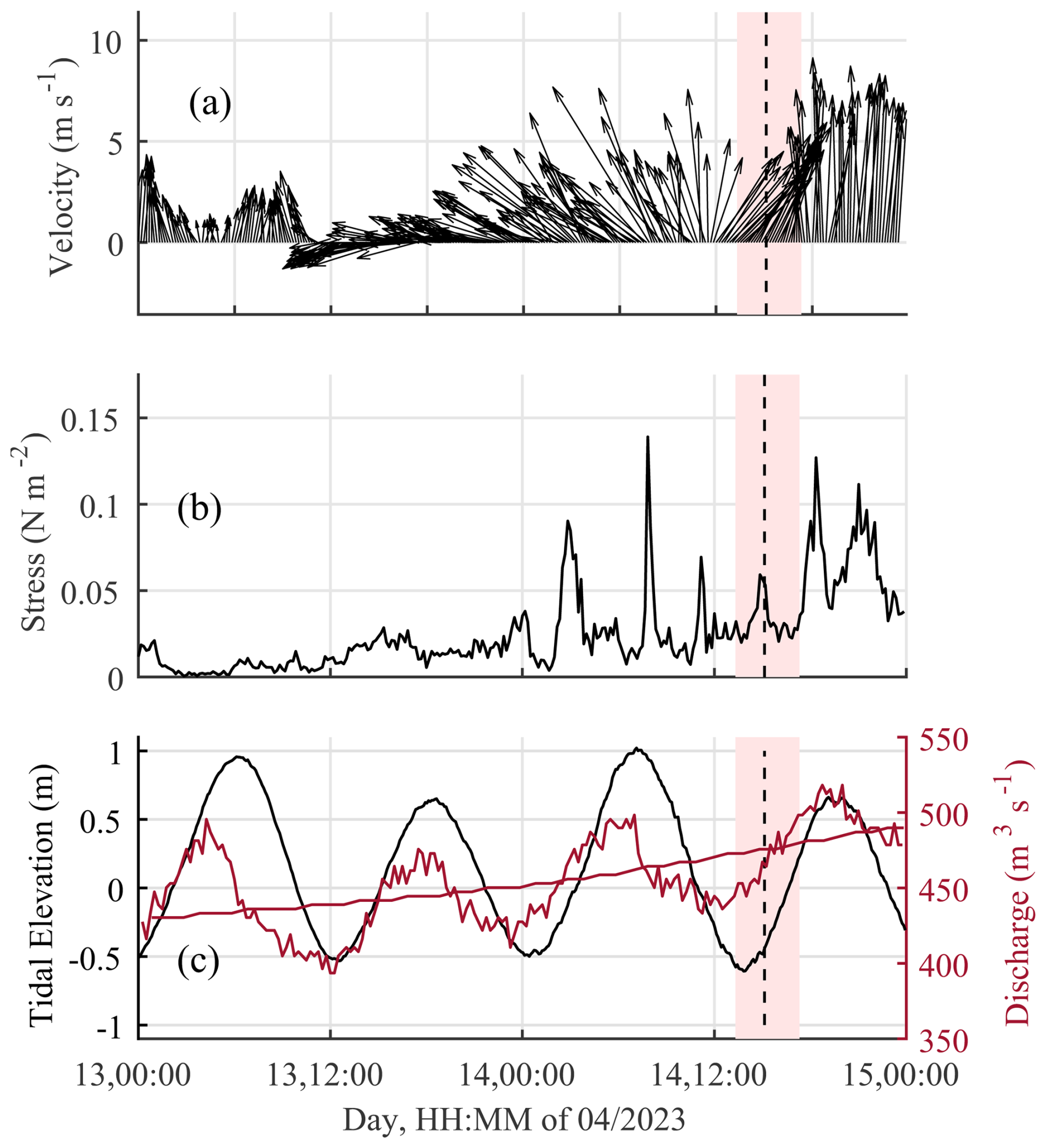
Figure 2 Time series of: (a) wind vectors for 2 d around the data collection period; (b) total wind stress estimated using the COARE 3.6 algorithm; and (c) measured tidal elevation (NOAA station 8661070, black line) and recorded (solid red line) and tidally corrected (dashed-dotted red line) river discharge (USGS station 02135200). Vertical black dashed line represents the time of plume front arrival and the red shaded area denotes the data collection period.

3.2 Near Surface Temperature Structure

The time series of both raw (at 2 Hz) and smoothed (using a 180-point/90 s moving averaging window) thermistor array data are shown in Fig. 3a and b, respectively. The same smoothed data, gridded as a function of time and elevation, are displayed in the form of a contour map in Fig. 3c. Initially the near surface temperature ranged from 18.5 °C at the surface to 17.5 °C towards the bottom of the array (2.82 m below the sea surface). The arrival of the plume front (15:07 UTC) is identified as the time when all temperatures from all depths collapse and shift to a higher temperature. This time corresponds to ∼ 1.9 h after LW, when the mean temperature over the top 3 m of the water column shifted from 18.3 to 18.7 °C. The near-surface mean temperature gradient, defined as the difference between the bottom and top sensor temperatures, divided over their separation distance (2.82 m), was ∼ 0.4 °C m⁻¹ until approximately 15 min prior to the arrival of the front. Then it dropped to 0.1 °C m⁻¹, increasing over time to almost 1.0 °C m⁻¹ toward the end of the data collection period, some 2.4 h after the plume front passage (see Fig. 3c). As seen from the spacing of the 4 upper thermistor time series (Fig. 3b), the local vertical temperature gradient within the top 1 m of the water column increased from 0.1 °C m⁻¹ near the front to 1.4 °C m⁻¹ some 2 h later.

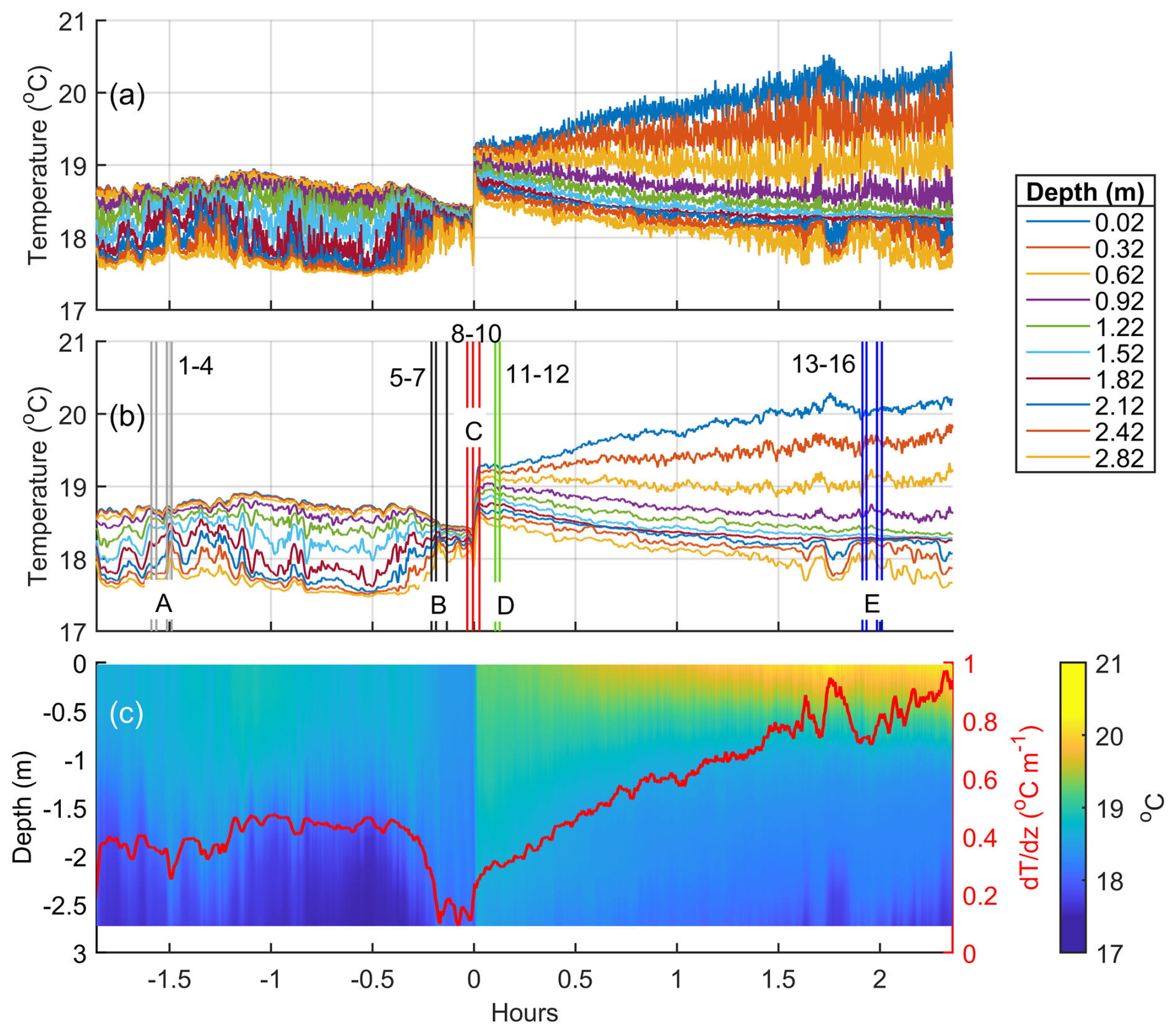
Figure 3 (a) Time series of the raw 2 Hz recorded temperatures for each individual thermistor located at depths varying from 0.02 to 2.72 m (see legend). (b) Same data as (a) but smoothed using a 180 point (90 s) moving average window. (c) Smoothed thermistor data (as in b) shown as a colored contour plot with temperature gradient (d$T/\mathrm{d}z$) superimposed (red line). The vertical lines in (b) identify the times of MicroCTD data collection with the numbers adjacent to them denoting the cast number; the letters (A to E) represent the sorting of the casts into groups (see text for details). Times are relative to the time of plume front arrival.

It is worth noting the oscillations shown in the temperature record in water depths 1.82 to 2.42 m during the periods −1.6 to −1.0 h. They have an amplitude of ∼ 0.2 °C and are visible in both the raw and smoothed data. Similar oscillations are seen later in the record after the plume front has passed through (see times 1.5 to 2 h). These latter oscillations are limited to the lowest three sensors corresponding to depths > 2 m and indicate potential internal wave activity.

3.3 Temperature – Salinity – Density Profiles

The 16 MicroCTD profiles of temperature and salinity collected during this study were used to estimate water density utilizing the TEOS-10 (IOC et al., 2010) model. The time of each profile in relation to the front arrival is shown in Fig. 3b. Based on cast time in relation to the time the front passed over the sensors, the profiles were sorted into 5 distinct groups. Casts 1–4 (group A) represent conditions before (∼ 1.6 h) the arrival of the front, when the plume's leading edge was at some distance from the data collection site, while casts 5–7 (group B) represent conditions just before (∼ 10 min) the plume's front passed over the sensors. Data from casts 8–10 (group C) correspond to when the plume front was exactly over the station. After the front's passage, casts 11–12 (group D), provide an insight of the conditions in the interior of the plume but near the front (some 5–6 min after). Finally, casts 13–16 (group E), show the structure of water properties from the interior of the newly arrived plume well after (∼ 2 h) the front had gone by.

The raw MicroCTD data are shown in a T-S diagram (Fig. 4) with different colors for different groups. Three distinct water masses can be identified corresponding to: (i) ambient deep water, (ii) a slightly less dense water mass representing a pre-existing water mass, presumably from the previous tidal cycle, and (iii) that of the newly arrived, warmer fresher plume. Each water mass is characterized by a certain range of T and S with these two parameters exhibiting an almost linear T-S relationship but with different slopes.

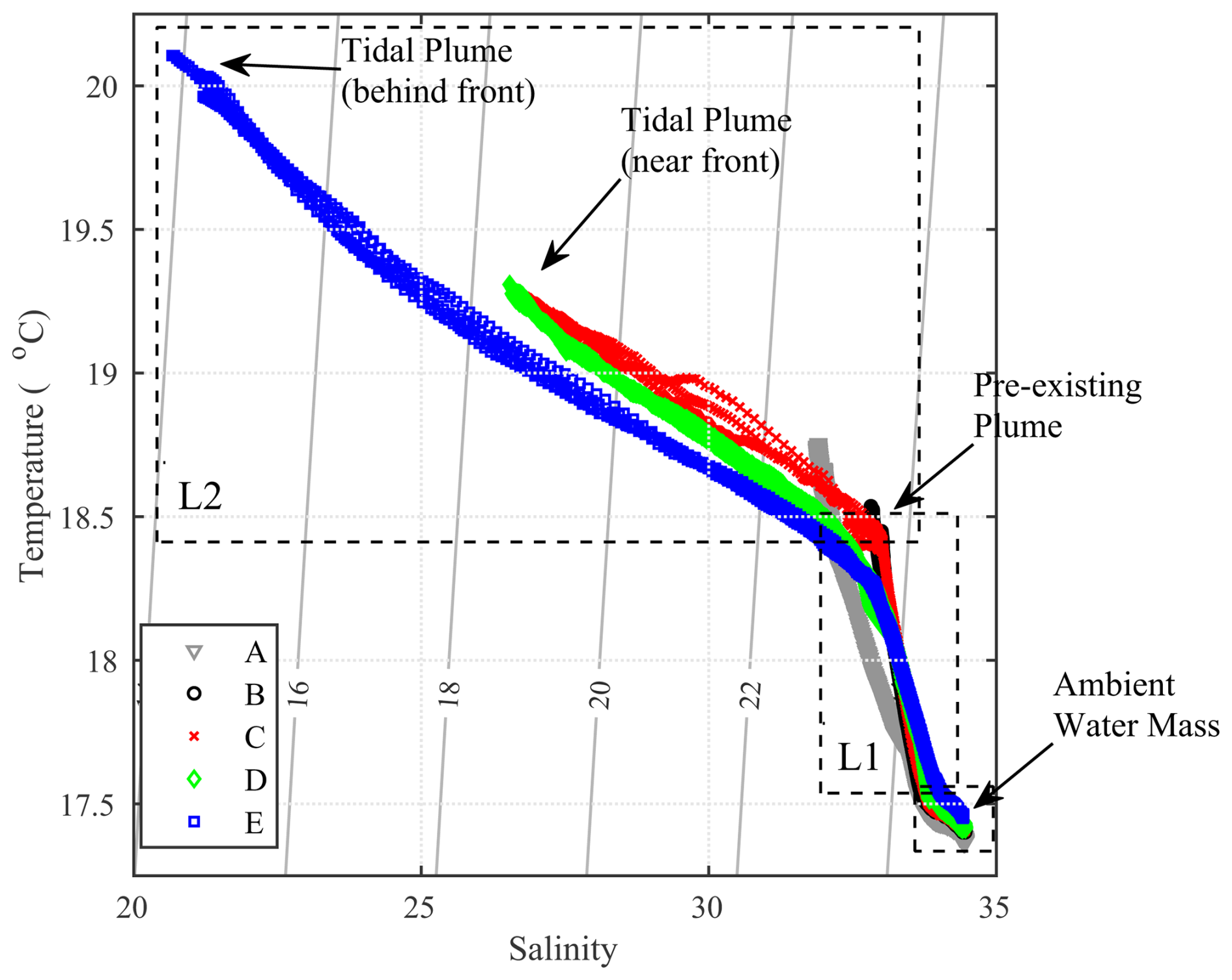
Figure 4 T-S diagram of the MicroCTD profile data collected during this study color-coded according to the group (A to E) they belong to (see text for details). The three dashed line boxes outline regions of the T-S space corresponding to the newly arrived layer (L2, top left), pre-existing (L1, middle box), and ambient (bottom right) water masses. End-members are indicated with arrows.

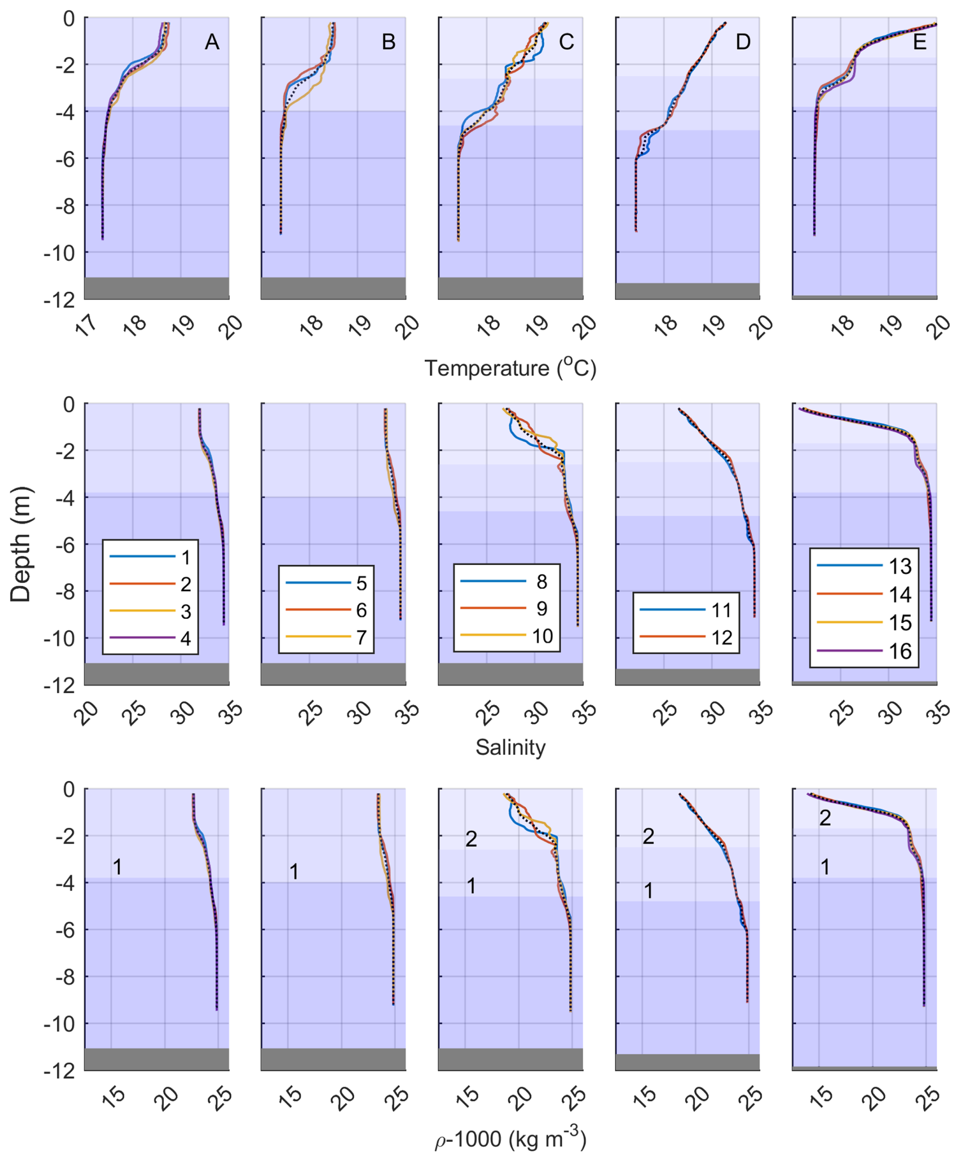
Figure 5 Individual profiles (1 to 16) of temperature (T), salinity (S), and density (ρ) arranged in different panels by group (i.e., 5 columns for groups A to E). Profiles within each group correspond to a different location/distance from the plume front (see Fig. 3b). Black dashed lines indicate averaged profiles for each group. Different shades of blue, from darker to lighter represent the different water masses: ambient, pre-existing plume (layer 1), and new plume (layer 2), respectively. For the depths of each layer see discussion in Sect. 4.

The vertical extent and structure of these water masses are displayed in the individual profile plots of temperature, salinity, and derived density (Fig. 5), separated by group. Group A and B profiles exhibit a consistent single step structure, while group C profiles show a two-step pattern that appears to persist in the profiles corresponding to groups D and E. These patterns are present in both temperature and salinity, something not surprising given the linear relationship between T and S (see Fig. 4).

Initially, in group A and B the uppermost layer (< 2 m) displays temperature, salinity, and density levels of approximately 18.7 °C, 32, and 1023 kg m⁻³, respectively. Meanwhile, the ambient bottom layer conditions (> 6 m) remain relatively stable, with temperature ∼ 17.3 °C, salinity 34.4, and density 1024.8 kg m⁻³. This is also clearly delineated in the T-S diagram shown in Fig. 4. As the front passes through, a sudden rise in surface temperature is observed by approximately 0.7 °C; the water temperature kept increasing with time until the end of data collection (a total of 1.5 °C increase over a period of ∼ 2 h). A similar abrupt shift toward lower values is seen in salinity. At the time of the front's arrival (group C) salinity reduces by approximately 5, eventually reaching a decrease of 12. In terms of density, the arrival of the front is associated with a decrease of 4 kg m⁻³, reaching densities of 1019 kg m⁻³ near the sea surface (< 2 m). In the interior of the plume (groups D and E) fresh, lighter water was recorded with surface water densities close to 1014 kg m⁻³.

3.4 Flow Structure

During the ∼ 4 h of data collection, a total of 27 averaged velocity profiles (ensembles) were collected using the AD2CP. The east (u) and north (v) components of the flow were rotated to local across- (u^′) and along-front (v^′) components (i.e., u^′ is along the direction of front propagation and v^′ transverse to the front propagation direction, see Fig. 1c). The coordinate system for this rotation was determined from drone imagery (see Fig. 12 in Sect. 4.3) with the direction of the cross-front (u^′) component established as 50° N. The vertical structure of the across- (u^′) and along-front (v^′) components is presented in Fig. 6a, b, in the form of contour plots. The vertical dashed line in Fig. 6 indicates the time of the front arrival as determined from the temperature profiles shown in Fig. 3.

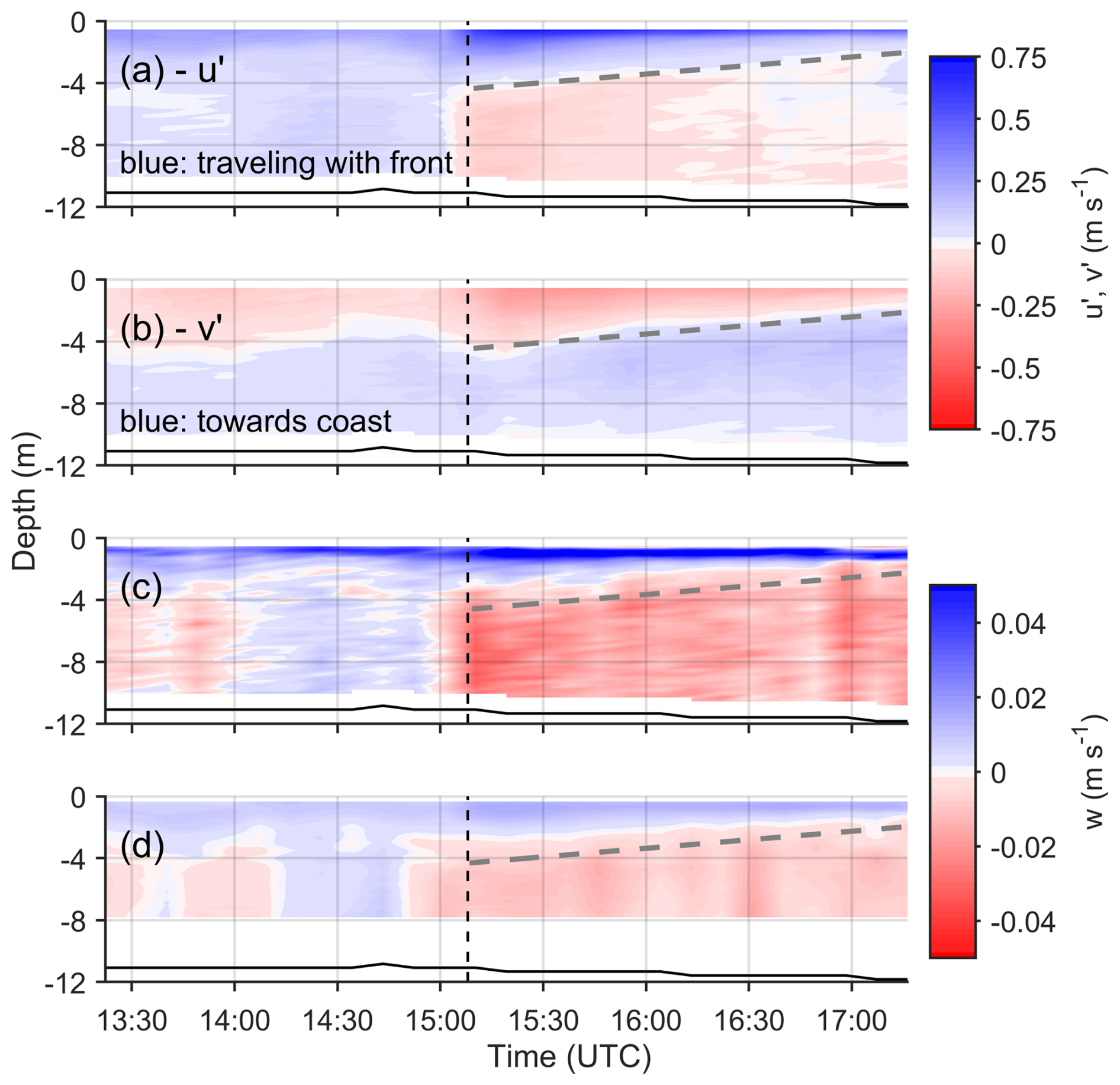
Figure 6 Vertical and temporal distribution of averaged current velocity components: (a) cross-front velocity component, u^′ (i.e., in the front propagation direction), (b) along-front velocity component, v^′, positive toward the coast (i.e., transverse to the front propagation direction), (c) vertical (w) component from the 4 beam BB data, and (d) vertical (w) component from the 5th beam. Data in (a), (b) and (c) represent an 8.53 min average while in (d) the average is 4.27 min. Vertical dashed lines indicate the time of front arrival; total water depth is shown as a solid black line. Note the different velocity scales for the horizontal and vertical velocities. Slanted grey dashed line indicates position of reversal of u^′ flow at base of plume (i.e., $u^{\prime }(z,t)=\mathrm{0}$).

Before the arrival of the front, the across-front (u^′) flow velocity (Fig. 6a) is uniformly positive throughout the water column with a depth averaged value of ∼ 0.10 m s⁻¹. With the front's arrival, the upper layer-averaged flow intensifies to ∼ 0.28 m s⁻¹ and then diminishes over time to ∼ 0.07 m s⁻¹, toward the end of the data collection period. During this time, a return flow develops under the surface layer with a vertically averaged (within the return layer) velocity that ranges from approximately −0.10 m s⁻¹ immediately after the arrival of the front to −0.02 m s⁻¹ toward the end of the data collection period. The observed flow pattern resembles that of estuarine circulation, and it is clearly associated with the arrival of the new plume. Estimates of the vertically (by layer) and temporarily (from the time of the front arrival to the end of the record) integrated velocities indicate upper- and lower-layer velocities of 0.174 and −0.044 m s⁻¹, respectively. Multiplying by the respective average layer depths of ∼ 2.5 and ∼ 9.0 m we obtain fluxes of 0.43 and 0.39 m³ s⁻¹ per m width, a difference of ∼ 10 % from their mean value.

The along-front flow component v^′ (Fig. 6b) shows a pattern of offshore (negative) flow near the surface and onshore directed flow below. This pattern is consistent before and after the arrival of the front with the flows being slightly intensified during the latter period. The mean velocities of the offshore directed upper layer are $\sim -$0.05 and $\sim -\mathrm{0}$.07 m s⁻¹ before and after the front arrival while those of the onshore (positive) directed bottom layer are ∼ 0.06 m s⁻¹ before the front arrival, doubling to ∼ 0.13 m s⁻¹ after that time. The increase in velocity at this time could be due to errors in defining the along-/across-front coordinate system, undulation of the front as it is not linear (see Fig. 1c), or tidal influence.

In the along-front propagation direction (u^′ > 0) the plume (surface layer) exhibits a shallowing over time (Fig. 6a, see slanted dashed line) with its base starting at ∼ −4 m when the front arrives and linearly shifting to ∼ −2 m at the end of the data collection period. This is likely due to radial expansion, but it could also be related to the formation of the trailing front, as described in a semi-analytical model of a radial supercritical plume forced by a constant discharge (Garvine, 1984). This shallowing over time suggests that for each time step (t) there is a depth level z(t) where u^′ reverses over a short time (dt) around t. At these times and depths d$u^{\prime }\left(z\right)/$dt is < 0 implying a local along front velocity divergence (d$u^{\prime }\left(z\right)/$dx> 0) at that elevation. Although continuity arguments would suggest that such divergence should drive vertical currents, the observed patterns shown in Fig. 6c and d are not easily explained using such arguments.

Two values of vertical velocity are available: (i) a value estimated from combining the 4 slanted BB beam radial velocities (Fig. 6c), and (ii) from the 5th beam radial velocity (Fig. 6d). Both vertical velocity estimates agree qualitatively, although the BB velocities show slightly higher values. The 5th beam radial velocities are considered more accurate as they do not suffer from the potential of contamination from the horizontal velocities due to tilt errors. Both records show a consistently positive (upward) flow close to the sea surface (< 2 m) for the whole period of data collection. Farther below just before and after the front's arrival negative velocities are seen, of the order of 0.02 m s⁻¹ (Fig. 6d), which persist all the way to the seabed. The depth of the vertical flow divergence (d$w/$dz< 0) appears to be shallower than that of $u^{\prime }\left(z\right)\approx \mathrm{0}$ (see slanted dashed line in Fig. 6) a depth where a consistent downward vertical flow is present.

3.5 Acoustic Backscatter

Acoustic returns include scattering by both turbulent salinity microstructure and particles in suspension (Lavey et al., 2013). Our AD2CP data lack sound spectral characteristics to allow for separation of the different backscattering sources. Furthermore, the acoustic frequency of 1 MHz falls in the region where both salinity microstructure and fine sediment-induced backscatter are equally important (see Fig. 2 in Lavey et al., 2013). Despite these limitations, acoustic backscatter data provide qualitative information describing the conditions during the data collection period. Figure 7 shows a time series of the intensity of the return acoustic signal (16 s averages) from both the HR 5th beam (Fig. 7a, vertical resolution 0.04 m, sampling frequency 8 Hz) and transducer 1 of the broadband (BB) array of the sensor (Fig. 7b, vertical resolution 0.25 m, sampling frequency 1 Hz). The HR return (Fig. 7a) does not extend to the seabed, unlike the BB transducer 1 data (Fig. 7b). Both data sets were corrected for geometric spreading and attenuation due to water absorption. Three major patterns are evident: (1) very high acoustic intensity at the time of the arrival of the front, presumably due to particulates and detritus accumulated in the front convergence zone; (2) increased acoustic backscatter near the sea bed that is confined at depths > 6 m prior to the arrival of the plume expanding to shallower depths (∼ 4 m) after the arrival of the front, especially toward the end of the time series; (3) increased intensity near the sea surface after the arrival of the plume that expands to deeper depths over time. The patterns described in (2) and (3) lead to the development of a lower backscatter region in mid-waters with a vertical extent that reduces over time after the arrival of the plume, suggesting a merging of the top and bottom high backscatter layers. In the region of lower backscatter intensity, prior to the arrival of the plume, we see evidence of internal waves (IW) with periods varying between 5 and 9 min. These IWs correspond to the times and depths (∼ 2 m) of the IWs identified in the lower sensors of the thermistor array (see Fig. 3b). No clear evidence is present for the period after the arrival of the front suggesting minimal, if any, role of flow instabilities in mixing processes.

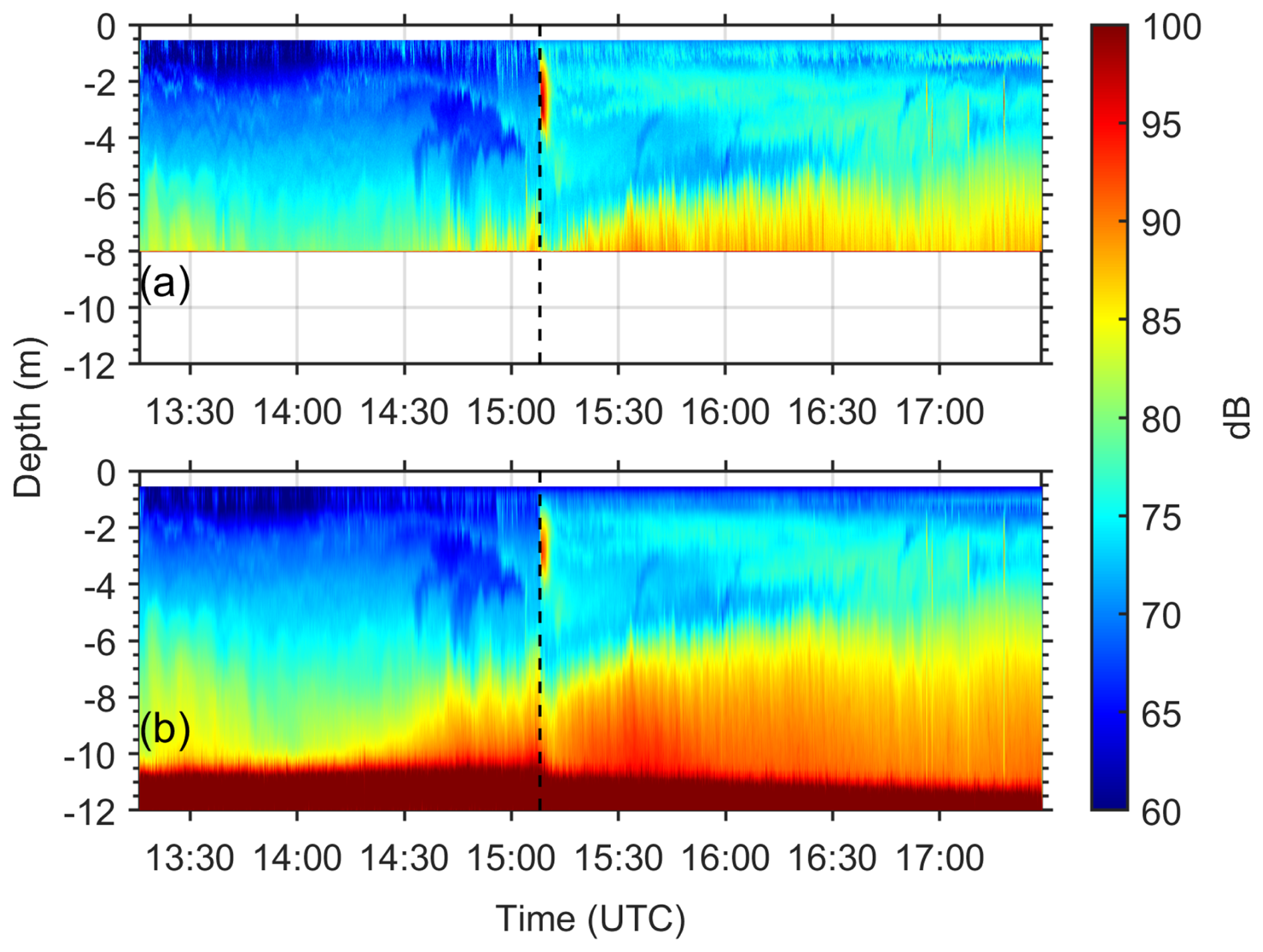
Figure 7 Time series of acoustic backscatter profiles corrected for geometric spreading and water attenuation. (a) From the HR 5th beam record with a vertical resolution of 4 cm, extending to ∼ 7.5 m depth; (b) from one of the Broad Band transducers (beam 1) extending all the way to the sea bed (vertical resolution 25 cm). Both records are 16 s averages of individual pings collected at 8 and 1 Hz for the HR and BB transducers, respectively.

3.6 Tidal Dynamics

The short record length (∼ 4 h) of the time series shown in Fig. 6 does not allow resolution of the tidal signal using harmonic analysis. Instead, the mean velocities from a total of 80 ensembles from 64 stations occupied during the study period are utilized. These stations are in the general area of the sampling site (see Fig. 8d) and the data were collected at different times over a period of ∼ 5 tidal cycles from 12 to 15 April 2023. The assumption made here is that the spatial variability of the tidal signal in the area is not significant. Only depth-averaged velocity data from water depths > 4.5 m are used in the analysis to ensure that the tidal current estimates are not influenced by plume-associated flows. This depth was defined based on the CTD profiles (see Fig. 5), and estimates using small variations in the selection of depth did not show significant changes in the results. The harmonic analysis was carried out for the two horizontal flow components using only periods corresponding to the semi-diurnal (M₂) and diurnal (O₁) constituents. Resolution of more semi-diurnal (i.e., S₂ etc.) or diurnal constituents is not possible due to the length of the time series and all energy from adjacent frequencies are included in the two components used in the analysis. In Fig. 8a and b the reconstructed time series of the tidal flows are shown together with the velocity data used as input in the least-squares analysis.

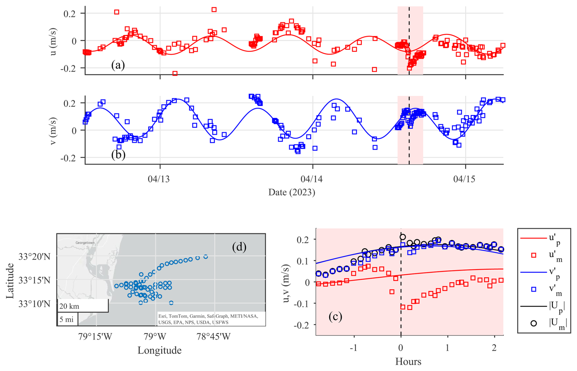
Figure 8 Time series of (a) east (u) and (b) north (v) bottom-averaged (depths > 4.5 m) velocity components from all stations occupied during the period 12–15 April 2023. The reconstructed tidal flow, shown as a solid line, was developed using the results of harmonic analysis at semi-diurnal and diurnal frequencies. The shaded area indicates the period station TS2 was occupied. (c) Close up of the measured and predicted tidal flows with time in hours relative to the time of plume front arrival rotated in across-front (u^′) and along-front (v^′) components; subscripts m and p denote measured and predicted flows, respectively. (d) Map showing the spatial distribution of the stations used for the tidal analysis.

The M₂ and O₁ amplitudes estimated were 0.06 and 0.01 m s⁻¹ for the east (u) component and 0.13 and 0.03 m s⁻¹ for the north (v) component of the flow. The corresponding relative phases were 205.3 and 69.3° for u and 60.3 and 233.7° for v. The overall mean tidal flow values were −0.03 and 0.07 m s⁻¹ for u and v, respectively. This mean flow is included in the tidal predictions shown in Fig. 8.

In Fig. 8c the predicted tidal flows and measured velocities are shown in across- (u^′) and along-front (v^′) coordinates. The along-front component (v^′) seems to follow the tidally predicted component most of the time. On the other hand, the across-front component (u^′) shows the largest deviation from the predicted tidal velocity in response to the tidal plume. The largest deviation occurs at the time of the front arrival (negative return flows) and diminishes over time. This confirms that although the along-front flow (v^′) in the lower layer is predominantly tidal, the cross-front component (u^′) is mainly the result of the arrival of the plume.

3.7 Turbulence Dissipation

Figure 9a shows turbulent kinetic energy (TKE) dissipation rate (ε_k) profiles estimated from the AD2CP vertical beam radial velocities using the second-order structure function (SF) method (see Sect. 2.2). The gaps seen in the profiles at mid-water levels are because of interference between two successive pulses and are a result of the shallow operating depth of the AD2CP. These data failed the MSPE (< 5 %) error criterion, as did some other data as shown in the figure.

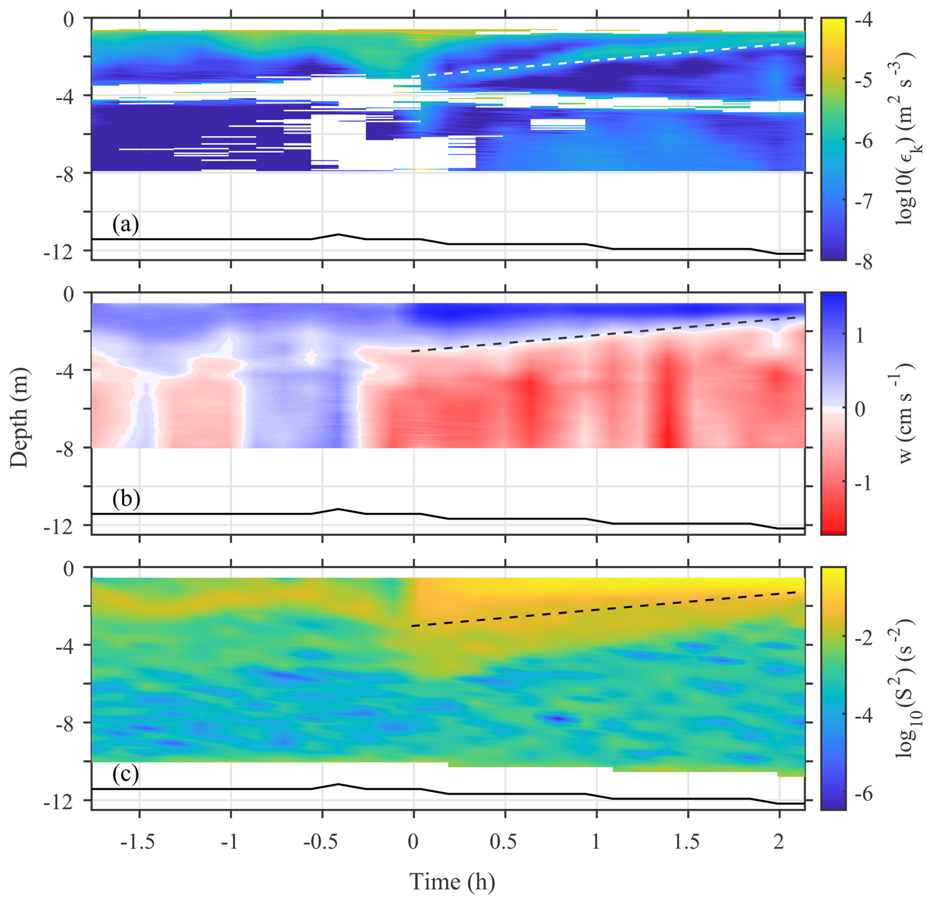
Figure 9 Time series of vertical distribution of: (a) Dissipation rate (ε_k) estimated from the AD2CP 5th beam HR radial velocity profile using the structure function (SF) method (see Sect. 2.2), derived from all 27 of the AD2CP 4.27 min ensembles. (b) Mean vertical velocity estimated after waves were removed using an EOF method (Zeiden et al., 2023). (c) Log of the square velocity shear (S²) estimated from the horizontal velocity components shown in Fig. 6. Dashed line is used to identify the location of vertical velocity divergence in all panels.

Prior to the front's passage, dissipation rates near the surface (< 2 m) are relatively high, of the order of 10⁻⁵ m² s⁻³ and decrease with depth down to 4 m. At greater depths (> 4 m) dissipation rates remain relatively constant and < 10⁻⁸ m² s⁻³. After the passage of the front, the dissipation rates exhibit a more complex structure, with high values near the surface as expected, reducing to 10⁻⁷ m² s⁻³ at greater depth and then increasing again (secondary peak) before decreasing again toward the 4 m depth. The secondary peak appears as a band of elevated TKE dissipation rates starting at ∼ 3 m immediately after the passage of the front and reducing in depth with time reaching approximately 1 m about 2 h after the front's arrival. In the lower water column (> 6 m) dissipation rates are lower before the arrival of the front than after. This is attributed to benthic boundary layer processes and increased near bed total current speeds mainly because of the tides (see Fig. 8c).

Although vertical velocities from the 5th beam were presented in Fig. 6d, the same data after correction for wave bias using the EOF method described in Zeiden et al. (2023) are shown in Fig. 9b. They show the same pattern as that of the raw velocities, i.e., persistent positive (upward) flow close to the surface and predominantly negative (downward) flows at greater depths after the passage of the front, but the velocity magnitudes are smaller by a factor of ∼ 2, never exceeding 0.02 m s⁻¹. As in Fig. 6, a clear divergence in vertical flow is evident that starts at ∼ 3.5 m depth just behind the front that linearly moves to shallower depths over time (see dashed line in Fig. 9b). As discussed earlier, this area of divergence seems to coincide with both the depths of elevated dissipation in the upper water column seen in Fig. 9a and with the region of relatively higher velocity shear (S) levels shown in Fig. 9c. It is worth nothing that the latter relationship is more with the base of the higher shear layer (bottom of tidal plume) and not necessarily with the highest shear levels, which are found closer to the surface (Fig. 9c).

4 Data Synthesis and Discussion

4.1 Plume Structure

The T-S-density profile results presented in Fig. 5 reveal a water column that transitions from a single-step to a two-step density structure. This suggests the presence of a pre-existing plume (hereafter referred to as layer 1) from the previous tidal cycle followed by the arrival of a newly discharged tidal plume (layer 2) that propagates above it. The system transitions from a two-layer model (ambient waters and pre-existing fresher water mass) before the arrival of the front to a three-layer model afterward. Although various investigators have used a particular isohaline to delineate a plume (i.e., S=21 in Kastner et al., 2018, S=27 in McDonald and Geyer, 2004 etc.) the T-S diagram shown in Fig. 4 suggests that the depth of the warmer tidal plume is defined by temperature and salinity values > 18.3 °C and < 32.7, respectively. This depth is 2.9 m initially reducing to 1.9 m toward the end of the data collection period. We quantitatively estimated the plume depth using the generalized equation of Arneborg et al. (2007), after modifying it for a three-layer structure (see Appendix A). The estimated depths for the pre-existing (D₁) and the new (D₂) plume are listed in Table 1 and provide each layer's vertical extent both before (t<t_f) and after (t> t_f) the front's arrival.

Table 1 Depths of pre-existing (D₁) and newly arrived (D₂) plumes for the times corresponding to the different group profiles.

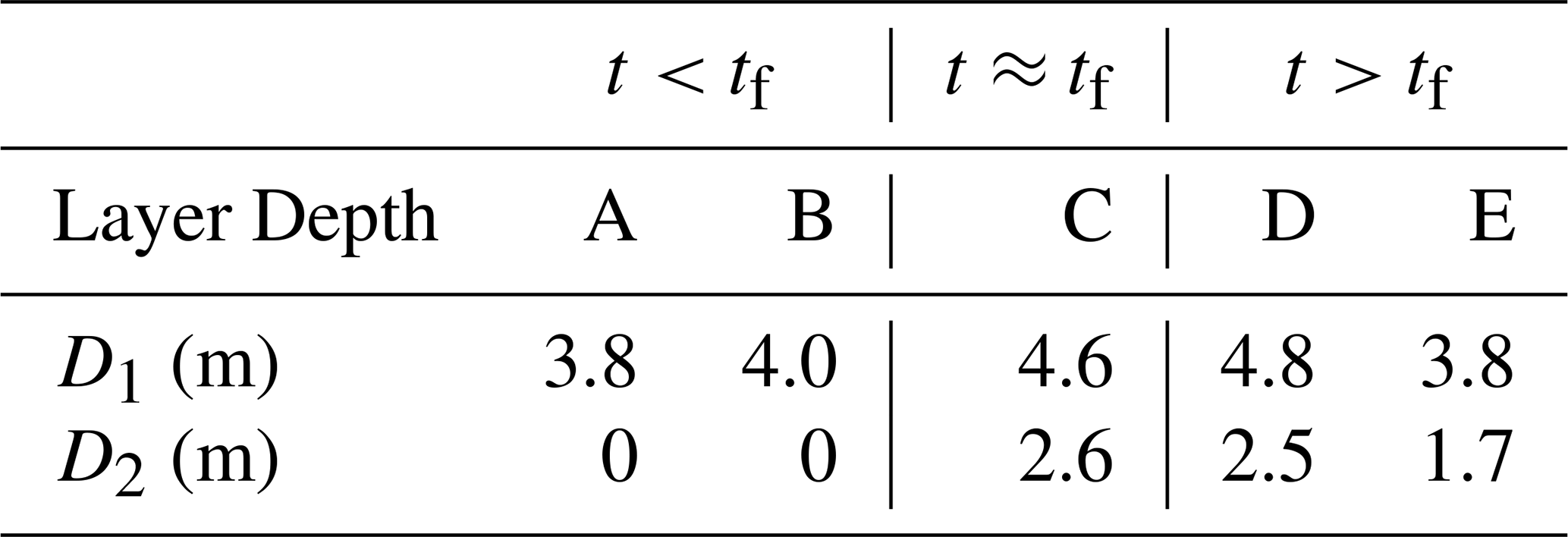
Initially, the pre-existing plume (layer 1) has a depth (D₁) of 3.8 m. The arrival of the newly discharged plume (layer 2) causes a depression in the interface between the pre-existing plume and the ambient waters by approximately 1 m, though this depression gradually diminishes over time. Over the course of the experiment, the depth of the newly discharged plume gradually decreased from 2.6 to 1.7 m, indicating a reduction by a factor of 0.75 over a period of ∼ 2 h. The D₁ and D₂ depths presented above appear to correspond to the 34 and 32.5 isohalines, respectively.

Utilizing the depths in Table 1 and the density profiles shown in Fig. 5, the mean water density within each layer was estimated and a conceptual schematic of the water column during the experiment is constructed and shown in Fig. 9. The pre-existing plume maintained a depth close to 4 m, with an average density of 1023.8 kg m⁻³ (S=33.1), overlying ambient ocean waters with a density of 1024.8 kg m⁻³ (S=34.3), while the new plume had an average density of 1020.7 kg m⁻³ (S=29.3).

4.2 Frontal Propagation

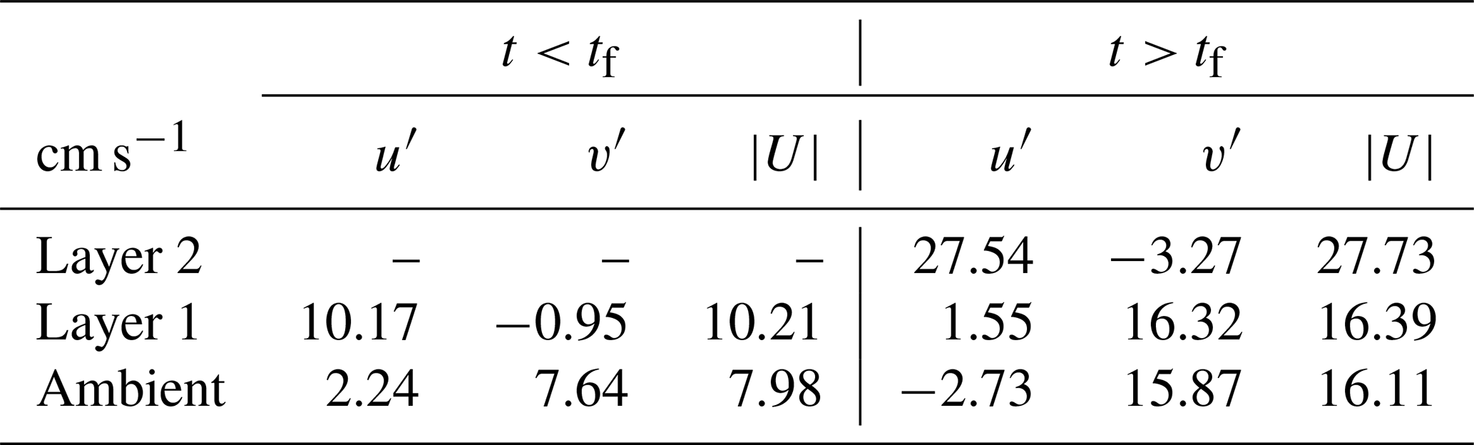
The absolute speed of the front was estimated from the upper bin of the AD2CP that was located at 0.55 m below the sea surface (U_s in Fig. 11) and successive photographs collected from a drone (Fig. 12). Both methods revealed a frontal propagation toward the ENE with an absolute front speed of 0.61 m s⁻¹. Although the propagation of the front, as shown in the imagery (z=0 m) is 50° N, the direction of the mean current of the upper bin (z = 0.55 m) of the AD2CP is 74° N. The water mass behind the front was moving with absolute speeds of 0.72 and 0.75 m s⁻¹ some 8.5 and 17 min after the front passage, respectively. The layer-depth averaged velocities of the front and plume behind it (denoted as U_f), after subtracting the layer-averaged velocity of the ambient layer, were 0.36 and 0.40 m s⁻¹, respectively, suggesting an overtaking velocity of 0.04 m s⁻¹. The vertically and time averaged across- (u^′) and along-front velocities (v^′) of the different layers identified in this study and schematically shown in Fig. 10 are listed in Table 2.

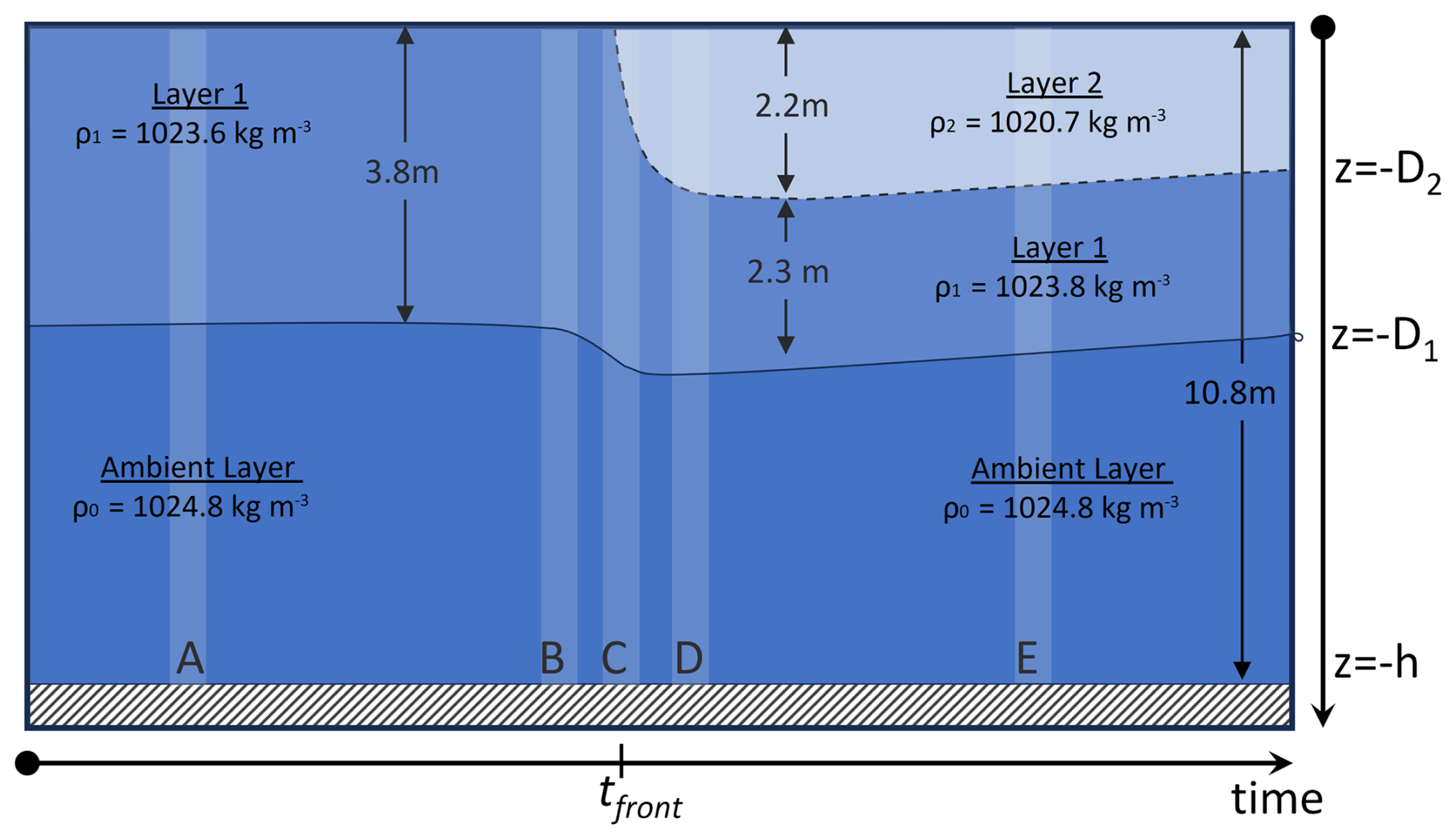
Figure 10 Conceptual model describing the structure of the water column throughout the data collection period. Initially a 2-layer structure is present (t < t_f) where an upper layer of depth D₁ and density ρ₁, presumably from a previous plume, is over ambient ocean waters with density ρ₀. The front of a newly discharge tidal plume of depth D₂ and density ρ₂ arrives at t=t_f, contributing to the creation of a 3-layer structure. The vertical shaded bands denote the time/relative location of the microCTD profile groups shown in Fig. 3b.

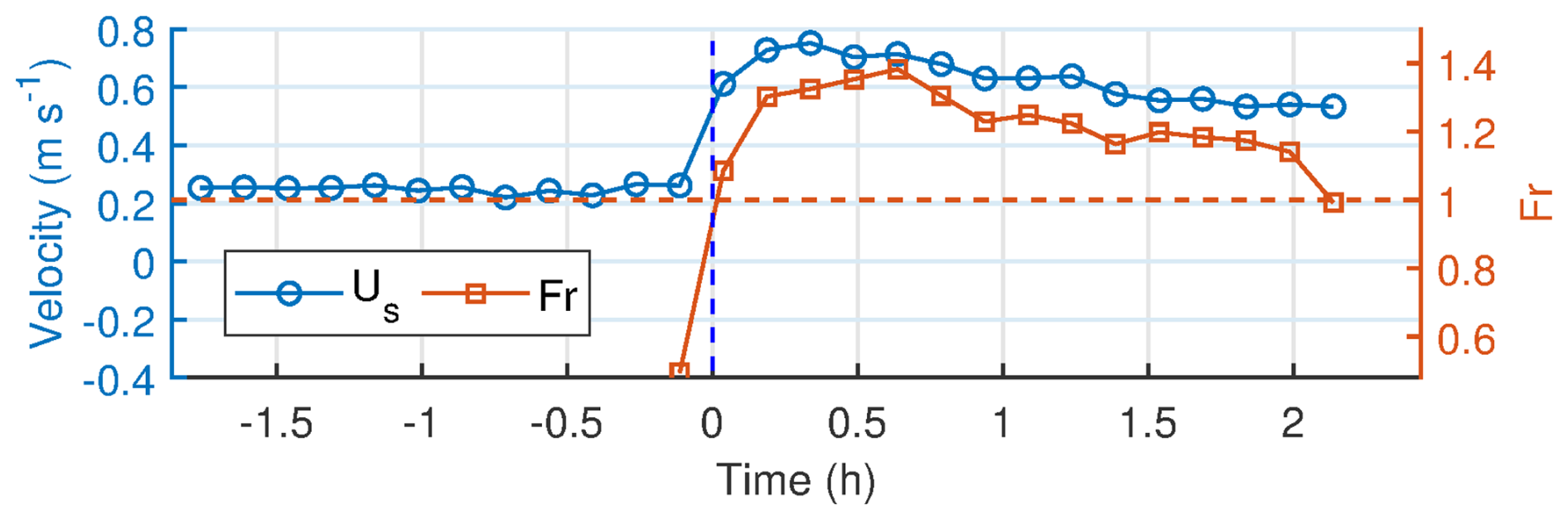
Figure 11 Near surface currents (U_s) before and after the arrival of the plume measured by the first bin of the AD2CP (z=0.55 m) and Froude number (Fr) variability inside the newly arrived plume.

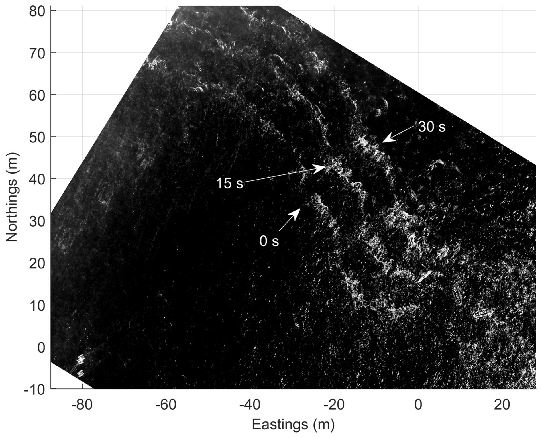
Figure 12 Composite image created from the superimposition of three orthorectified aerial images of the front obtained at three different times, 15 s apart. Image rectification based on the drone GPS data while lens distortion was accounted for using an earlier version of the calibration package of Bouguet (2022).

Table 2 Vertically integrated and time averaged across-front (u^′), along-front (v^′) and total magnitude ($\left|U\right|$) velocities (in cm s⁻¹) for each layer shown in Fig. 10 prior to (t<t_f) and after (t>t_f) the arrival of the front. Layer 2 is the newer plume, layer 1 is the pre-existing plume, and the waters below layer 1 are the ambient layer.

The reduced gravity g^′ and the mean depth of the layer of the plume (layer 2, D₂) were found to be 0.034 m s⁻² and 2.2 m, respectively. Based on these values a frontal Froude number ($Fr=U_{\mathrm{f}}/(g^{\prime }{D}_{\mathrm{2}}{)}^{\mathrm{1}/\mathrm{2}}$) of 1.32 is estimated. This value is between the theoretical value of 1.42 expected for a freely propagating gravity current (von Karman, 1940) and the value of 1.19 suggested by Huppert and Simpson (1980). The flow remained supercritical (Fr>1), although diminishing over time for 2 h after the front passed over the station (Fig. 11). Using an average water depth of 11.5 m and the frontal speed of 0.36 m s⁻¹, a frontal Reynolds number ($R{e}_{\mathrm{f}}=\left(U_{\mathrm{f}}h\right)/\mathit{\nu }$ ) of 4.03×10⁶ is estimated, a value very similar to that found for the Merrimack River plume by Horner-Devine at al. (2013). The bulk-mixing coefficient (β, Simpson and Britter, 1979, 1980) was calculated to be 0.11, which is less than half of the value of 0.37 reported in Pritchard and Huntley (2000).

Although there are no direct observations of the spatial structure and spreading rate of the plume, the Sentinel image collected the day after the experiment (see Fig. 1) provides a snapshot in time of the plume shape and areal extent at that time. Assuming a semicircular shape as in Pritchard and Huntley (2006), the area of the plume (62 km²) was used to estimate the plume effective radius to be 4.4 km. Using the observed plume velocity averaged over 2 h past the front arrival of 0.33 m s⁻¹ (1.2 km h⁻¹) as a representative value of a linear spreading rate (see Pritchard and Huntley, 2006), then the change of the effective radius variability during the time elapsed between the front's passage from the sensors to the end of the data collection period (∼ 2 h) is ∼ 6.7 km. Assuming an instantaneous release of freshwater and conservation of mass, then the reduction of the plume depth over the 2 h of observation is estimated to be ∼ 0.43 m. This is an extreme value estimate assuming all river discharge occurred instantaneously at LW and there was not a continuous supply of fresh water. The shallowing of the plume observed is of the order of 0.60 (using the density profiles in Fig. 5) which is greater than the 0.43 value but reasonable given the uncertainties of these estimates.

4.3 Plume Flow Structure

As discussed in Sect. 3.4, the flow structure along the direction of the plume propagation is characterized by the development of a return flow under the plume (Fig. 6a) resembling that of estuarine circulation. The strength of the return flow reduces over time as the plume spreads. Tidal analysis (Fig. 8c) clearly shows that the predicted tidal velocity component along this direction is weak (from 0 to 0.05 m s⁻¹), and the return flow deviates significantly from the expected tidal signal. Crude 2-D water mass conservation analysis (per unit width of water column) showed a closure within 10 % supporting the argument of the development of a plume-driven return flow. Although opposing flows underneath tidal plumes have been described before (e.g., Horner-Devine et al., 2009) these represented ambient water conditions into which the plume was discharged. Shipborne flow observations on the Merrimack River by MacDonald et al. (2007) did not capture such return flows. In the same area, Spicer et al. (2022) observed return flows under the detached Merrimack River plume, but those were attributed to the tidal patterns of the area and not the plume itself. More recently, Delatolas et al. (2023) reported return flows that were thought to be associated with the frontal convergence zone reaching all the way to the sea bed; however, since the study was focusing on mixing and not flow structure, no evidence was presented to identify the role of tides as was the case in Spicer et al. (2022) for the same location.

In another study, Orton and Jay (2005) presented evidence of return flows under the Columbia River tidal pulse (see Fig. 2a therein) under upwelling-favorable winds and high river discharge (4900 m³ s⁻¹). The return flows extended all the way to the bed (∼ 20 m), as is the case in this study. Our observations also appear to be in close agreement with those of Solodoch et al. (2020) from the Mississippi River plume. They showed similar return flows under the plume, and they found these to qualitatively resemble the canonical density current structure for a gravity current propagating in stratified waters. As shown in the schematic of Fig. 10, in our case the new front is arriving into already stratified waters (layer 2), consistent with the arguments of Solodoch et al. (2020). The development of such return flows has implications on modeling and representation of tidal plumes, and most likely depends not only on river discharge and local water depth but also on the degree of stratification of the ambient waters prior to the arrival of the plume. One important finding of this study is how the shallowing of the base of the plume and the development of return flows can lead to areas of horizontal flow divergence, and possibly the development of vertical flow divergence, co-located with areas of local maxima in TKE dissipation rates (Fig. 9).

The along-front flow v^′ observed structure (Fig. 6b) of offshore (negative) flow near the surface and onshore directed flow below is attributed to tidal flow. The onshore (positive) directed along-front flow (v^′) shown in Fig. 6b seems to be explained by the tidal component as predicted using the tidal analysis (Fig. 8c). This is supported by the fact that the pattern is the same before and after the arrival of the front. The offshore (negative) directed upper layer flow most likely represents the radial spreading of the plume and the influence of the upwelling-favorable winds prevailing during this time. Analysis by Papageorgiou (2023) demonstrated that the vertical structure within the pre-existing plume (layer 1) resembles that of an Ekman layer, suggesting that the movement of the older plume is driven by the wind that is directed toward the NE (Fig. 2).

4.4 Mixing Processes

The density profiles (Fig. 5) from the periods corresponding to groups A to E were matched to corresponding mean velocity profiles (Fig. 6) to estimate buoyancy frequency (N) and shear (S, where $S^{\mathrm{2}}={\left(\frac{\partial u}{\partial z}\right)}^{\mathrm{2}}+{\left(\frac{\partial v}{\partial z}\right)}^{\mathrm{2}}$ ) for each group. The process included spline interpolation of the flow data (dz=0.25 m) to the elevations of the buoyancy frequency profiles (dz ∼ 0.01 m), and application of a 32-point moving average (∼ 0.32 m) prior to estimating gradients. The individual N and S estimates for each profile were then averaged for each group and the profiles are shown in Fig. 13 (top). The logarithm of 4N² and S² are plotted together. These profiles depict an alternative representation of the gradient Richardson number (Ri${}_{\mathrm{g}}=N^{\mathrm{2}}/S^{\mathrm{2}}$) so that S²>4N² represents Ri_g<0.25, suggesting that turbulence can mix the water column (Thorpe, 1987).

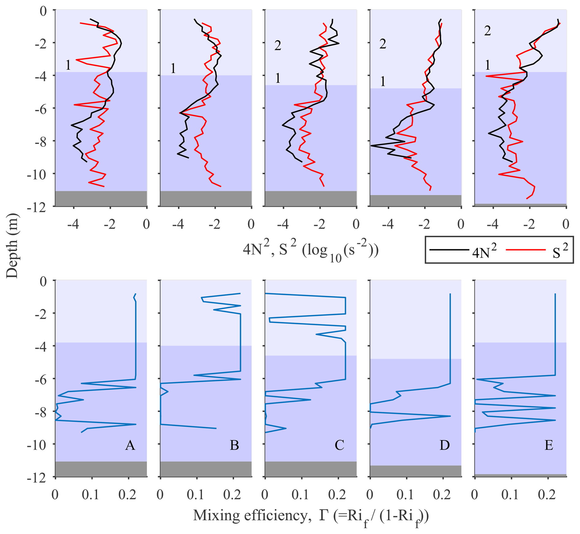
Figure 13 Top: Group (A to E) mean profiles of four times the squared buoyancy frequency (4×N²) and vertical shear (S²) estimated from the CTD profile shown in Fig. 5. S²>4N² represents Ri_g<0.25. Bottom: Mixing efficiency parameter (Γ) estimates using Eq. (5). The different shades and numbers 1 and 2 represent the different water masses identified (1 – pre-existing plume, 2 – newly discharged plume).

As expected, buoyancy (represented by 4N²) is generally highest within the plume layers, although it tends to stay elevated one to two meters below layer 1 (the pre-existing plume) for all but group E, which was furthest behind the front (Fig. 13, top panel, black line). Before the arrival of the front (group C), buoyancy is suppressed closer to the surface, then increases in the top 2 m (within layer 2) after the front's passage. Shear (S²) values also are highest within the plume layers, with broad patterns like those of buoyancy, although shear shows slightly less depth variability and a clearer near-bottom increase for all groups (Fig. 13, top panel, red line).

Mixing should be favorable where S²>4N², which is consistently the case for the lower part of the water column (depths > 6 m). This is not unexpected, as in this region stratification is relatively weak and bottom friction can generate shear. Near the sea surface, the $S^{\mathrm{2}}/\mathrm{4}{N}^{\mathrm{2}}$ ratio tends to oscillate around 1. Prior to the arrival of the plume (A and B) near the surface (< 2 m) there is a tendency for S²>4N² while farther below and within 2 m of either side of the interface with the ambient waters, buoyancy dominates (i.e., S²<4N²). The latter pattern persists even in group C although its vertical extent is limited to ±1 m around the interface. Once the front of the new plume arrives (layer 2, group C) buoyancy exceeds shear within the new plume. Later (D), buoyancy and shear appear to be balancing each other (i.e., S²∼4N²), suggesting a gradient Richardson number of ∼ 0.25. This balance is maintained within the newly arrived tidal plume (E), but buoyancy seems to be dominant within the pre-existing plume layer (layer 1).

Overall, the shear and buoyancy profiles indicate that conditions are most favorable for mixing in the top 2 m prior to the front's arrival, and in the lower plume layer right at the front. Mixing is also likely throughout the plume (particularly in the newer plume waters) after the front's passage. Stability dominates just beneath the plume, but below that conditions are again favorable for mixing, where stability is lower and shear is increasing near-bottom.

Mixing processes are examined using the `available overturn potential energy' (AOPE) in the water column, first presented by Dillon (1982) and later revisited by Smith (2020). The latter work presented an implementation method suitable for profile data with uneven vertical spacing, as is the case for our MicroCTD, which we follow here. The method sorts the density values of the profile and then estimates the relevant Thorpe scales (L_T). The regions of the water column where the cumulative sum of L_T becomes 0 define parts of the water column where overturning occurs (i.e., turbulence patches). The size of each turbulence patch (L_Q) is estimated, and a constant Thorpe scale is assigned to each of them. Using this method, we estimated the dissipation rate (ε_p) of turbulent potential energy (TPE) using:

$$\begin{array}{}\text{(5)}& {\mathit{\epsilon }}_p={\displaystyle \frac{(\mathrm{0.55}+\mathrm{0.45}m/\widehat{m})}{\mathit{\alpha }}}{L}_T^{\mathrm{2}}{N}_A^{\mathrm{3}}\end{array}$$

where α=4, $m/\widehat{m}$ is the slope ratio (m-ratio) defined as the slope of a linear fit of the raw data (m) over the slope of a linear fit to the sorted data ($\widehat{m}$, equivalent linear stratification, see Mater et al., 2015), and N_A is the equivalent buoyancy frequency derived from the equivalent linear stratification defined as:

$$\begin{array}{}\text{(6)}& N_A={\displaystyle \frac{\sqrt[\mathrm{2}]{\mathrm{2}\mathrm{AOPE}}}{L_T}}\end{array}$$

where AOPE is the change in potential energy before and after sorting (see Eq. (9) in Smith, 2020).

The ratio of the Thorpe scale (L_T), representing overturn, over the size of a turbulence patch (L_Q) where the overturn takes place, can provide an insight into the mixing mechanism (i.e., shear-flow vs. density inversion driven). This is called the L-ratio, and it has been empirically related to the m-ratio. An m-ratio of −1 represents what Smith (2020) defines as a “young” patch corresponding to conditions of purely buoyancy induced turbulence, while a value of +1 represents mixing by pure shear-driven turbulence. This parameter is a potential indicator of the relevant contribution of the kinetic and potential components in total turbulent energy and dissipation (Smith, 2020).

The vertical distribution of the Thorpe overturning scales for each one of the profiles, arranged by group, is shown in Fig. 14 (top). These plots appear to be more informative than the buoyancy and shear plots (Fig. 13) discussed earlier. The largest overturning scales are found near the bed with values ranging from 0.20 to 0.50 m. The smallest (∼ 0.20 m) near-bed L_T scales are found at group A, slightly increasing at group B prior to the arrival of the plume, and attaining their largest values (∼ 0.50 m) during and after the arrival of the new plume (groups C to E). Similarly high overturning Thorpe scales are seen near the surface, limited to depths < 1.5 m in group A. This layer of high L_T values deepens over time to 2.5 and 4.0 m for group B and C profiles, respectively. After the arrival of the new plume, there are very few near-surface L_T estimates, as the sorting of the density profiles did not identify any overturns, or the ones estimated were of the order of the vertical resolution of the CTD profiles (∼ 0.01 m) which approach the instrument noise level. In groups A to C no significant overturning is revealed in the region between the surface and bottom layers. The same results are shown in Fig. 14 (middle) where the extent of the regions of overturning (i.e., turbulence patches) are shown.

The slope ratio profiles (Fig. 14, bottom) suggest that the near bed overturning regions, described above, coincide with regions of ratios close to +1 suggesting shear flows being the main driving force. Near the sea surface the slope ratio values show a scatter from −1 to +1 for group A. The scatter reduces to the range −1 to 0 in group B, suggesting a diminishing contribution of shear flows. This narrow range continues to group C where slopes are between −1 and −0.5. It is worth noting that the areas of highest shear (S²) shown in Fig. 13 do not coincide with the regions of slope ratio +1 suggesting that the flow shear is not sufficient to create overturns within the plume in the presence of strong stratification.

Figure 15 shows the vertical distribution of the estimated TPE dissipation rates (ε_ρ, Eq. 5, Fig. 15 top) and density diffusion coefficient ($K_{\mathit{\rho }}={\mathit{\epsilon }}_{\mathit{\rho }}/N^{\mathrm{2}}$, Fig. 15 bottom). For comparison, the TKE dissipation rate profiles from the AD2CP (SF method, see Fig. 9) and the MicroCTD estimates are also shown on the same figure as black solid and red dotted lines, respectively. As discussed earlier (see Eq. 2) the ratio ${\mathit{\epsilon }}_k/{\mathit{\epsilon }}_{\mathit{\rho }}$ describes the mixing efficiency of the flow. Although the plots appear busy, general patterns emerge worth identifying. (i) The TKE dissipation rates (ε_k) from the instantaneous microstructure profiles and the averaged AD2CP HR radial velocities (see Sect. 3.7) show a general qualitative agreement. As discussed earlier and in Papageorgiou (2023) the SF method estimates are time-averaged quantities, while the microstructure estimates are those of individual instantaneous profiles. Nevertheless, all estimates show higher dissipation rates near the sea surface, diminishing with depth to 10⁻⁹–10⁻⁸ m² s⁻¹, values close to noise levels. (ii) Near the surface in groups A and B profiles, ε_ρ≪ε_k, by at least two orders of magnitude, suggesting Γ values ∼ 0.01 as suggested by Burchard and Hofmeister (2008). In group C, ε_ρ is smaller but similar order to ε_k indicating a higher mixing efficiency than in A and B. (iii) Near the bed, in the regions where the slope ratio was found to be ∼ +1, the TKE and TPE dissipation rates appear to be of similar orders of magnitude, making the argument of a mixing efficiency coefficient (Γ) with values between 0.2 and 1 plausible. (iv) Within the new plume, although relatively high TKE dissipation rates are estimated by both the SF method and the microstructure probe, the overturning analysis suggests limited vertical mixing. This discrepancy within the new plume could potentially be attributed to local anisotropic turbulence (Lewin and Caulfield, 2024) that does not contribute to vertical mixing and/or turbulence advection, however we are unable to assess that mechanism here. It is worth noting that the conditions and resulting mixing effects observed here resemble those described in studies associating stratification with tidal straining. Given the two-layer flow observed in the across-front direction (Fig. 6a), and the importance of tides to this plume system, mixing may be suppressed by enhanced density gradients due to advection of fresher surface water on the ebb tide. Rijnsburger et al. (2018) observed tidal currents rotating in opposite directions in the surface and bottom layers during neap tide and low winds off the Rhine River mouth, a phenomenon also predicted by a 3-D numerical model of this region (de Boer et al., 2006). This was observed in the far-field, so a slightly different regime given our high Froude number estimates, while our system may be more analogous to what has been observed in estuaries. Upwelling-favorable winds and the related Ekman transport could further reinforce this enhancement of freshwater advection in the across-front direction. The observations presented here represent neap tide conditions, which may also enhance stratification and reduce mixing and stirring processes (Rijnsburger et al. 2018; Simpson et al., 2005). To date, there have been few observational studies addressing the potential role of tidal straining in the context of river plumes. Furthermore, it should be noted that tidal straining describes the drivers for enhanced stratification but does not provide insights into the actual mixing processes themselves.

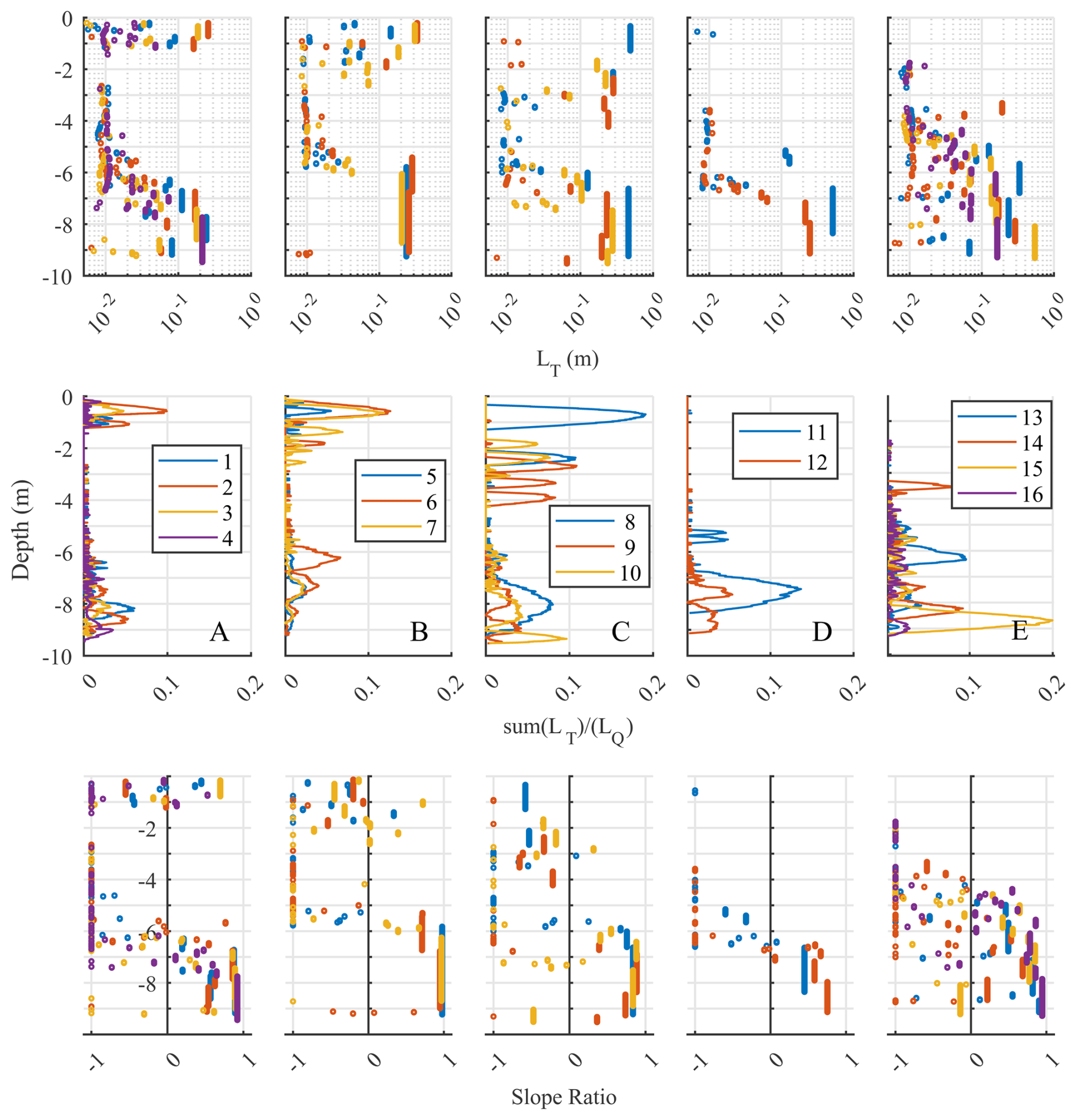
Figure 14 Results of the Smith (2020) method for assessing mixing using the water column turbulent potential energy. Top: Thorpe scales (L_T) estimated from sorting individual density profiles (see Fig. 5). Middle: Vertical extent of turbulence patches estimated from summing the estimated Thorpe displacements; the values shown are the sums normalized by the scale (length) of each individual turbulence patch. Bottom: Vertical distribution of the slope ratio indicating the potential mixing mechanism (see text for details). Each column corresponds to a different profile group (A to E) representing different times in relation to the time the plume front passed over the station.

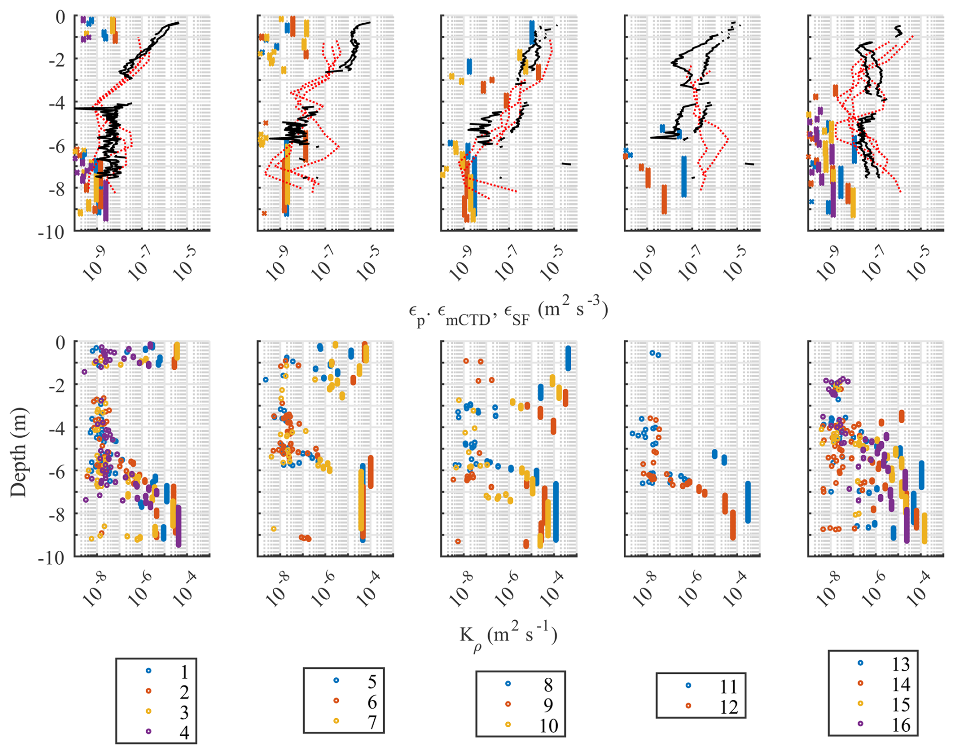
Figure 15 Results of the Smith (2020) method for mixing using the water column turbulent potential energy. Top: Profiles of (i) dissipation rate of turbulent potential energy (ε_ρ) using the Smith (2020) method (dots); (ii) TKE (ε_k) from the microstructure (MicroCTD) profiler (red dashed lines) and the AD2CP (black lines) after applying the Structure Function (SF) method (see Fig. 9a). Bottom: Density diffusivity (K_ρ) estimated using the Smith (2020) method (see text for details). Each column corresponds to a different profile group (A to E) representing different times in relation to the time the plume front passed over the station.

In summary, the vertically integrated layer estimates of TKE and TPE dissipation rates, along with density diffusivity, are listed in Table 3 for the different groups/times before (A, B), during (C) and after (D, E) the passage of the front.

Table 3 Layer integrated estimates of dissipation rate of TKE (ε_k), turbulent potential energy (ε_p), and density diffusivity (K_ρ) for the different regions before (A, B), at (C), and after (D, E) the plume front passage. The mixing efficiency parameter Γ estimated for the corresponding dissipation rates is also listed.

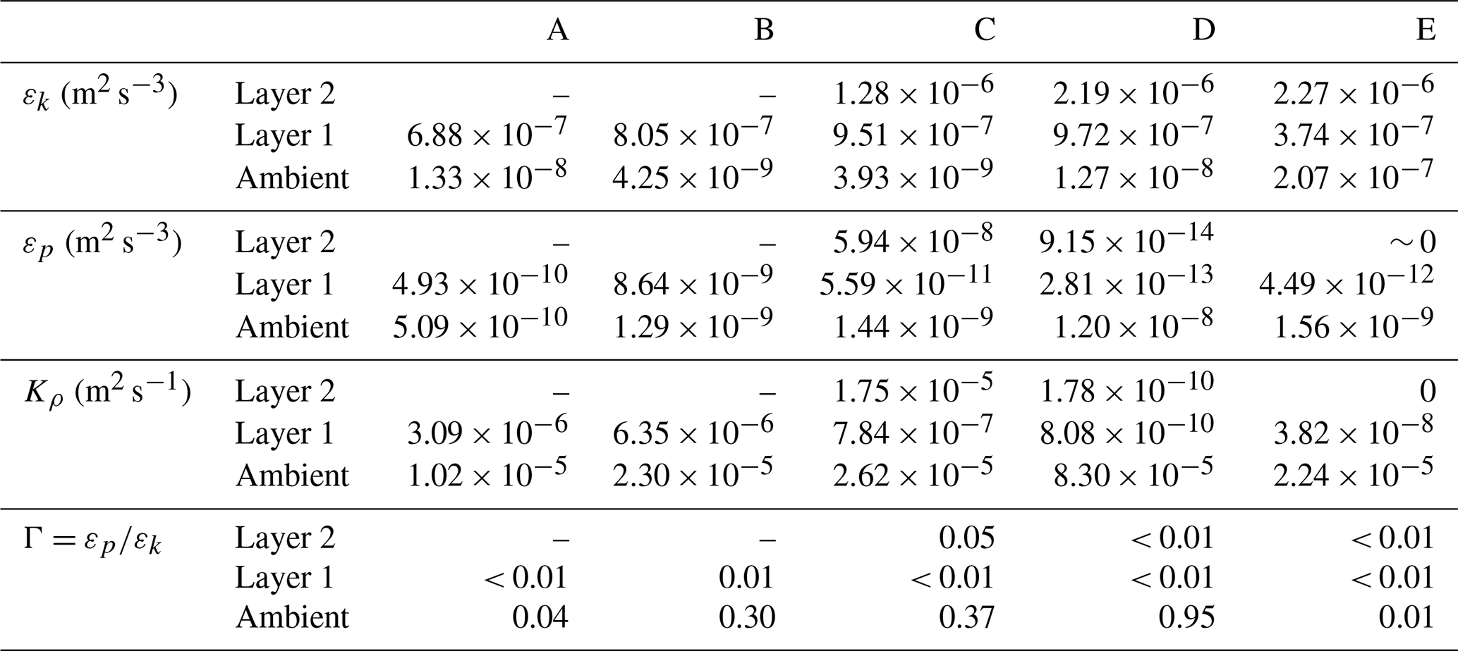
It is notable that within the plume (layer 2), density diffusivity is highest (∼ 10⁻⁵ m² s⁻¹) during the passage of the front (group C) and quickly reduces to ∼ 10⁻¹⁰ m² s⁻¹ soon after (group D) diminishing to zero some 1–2 h later (group E). This suggests vertical mixing is shut down behind the front despite the highly sheared flows occurring there (see Fig. 9c). The gradient Richardson number within the plume (layer 2, see Fig. 13 top) is ∼ 0.25 with corresponding squared buoyancy frequency (N²) values of 0.008 and 0.025 s⁻² for D and E, respectively. Using these values with the corresponding TKE dissipation rates listed in Table 3 we derive buoyancy Reynolds numbers (Re_b) of 273 and 90 for D and E, respectively. Imberger (1983, cited in Delatolas et al., 2023) suggested that when Re_b < 21 turbulence ceases to be isotropic as stratification suppresses vertical mixing. However, in their studies ε_k was on the order of 10⁻⁶ m² s⁻³ near the front and reduced to 10⁻⁸ m² s⁻³ behind it, while our results indicate a higher, almost constant dissipation rate of 10⁻⁶ m² s⁻³ within the tidal plume. This TKE dissipation trend is also noteworthy as it differs from the exponential decay observed in several other plumes (Orton and Jay, 2005; O'Donnell et al., 2008; Horner-Devine et al., 2013; Delatolas et al., 2023). Our diffusivity estimates at and behind the plume (C and D) appear to be even lower than those presented in Ivey et al., (2020) for Re_b ∼ =10 (see their Fig. 3) and our gradient Richardson numbers are high for pure convective mixing. Near the bed and within the ambient layer the TKE dissipation rate is extremely low (10⁻⁸ to 10⁻⁹ m² s⁻³) increasing to 10⁻⁷ m² s⁻³ at E. This increase is attributed to bottom boundary layer turbulence and increased tidal velocities over time as shown in Fig. 8c. Near bed density diffusivity appears to remain constant at ∼ $\mathrm{3}\times {\mathrm{10}}^{-\mathrm{5}}$ m² s⁻¹. In terms of mixing efficiency, mixing is more efficient in the bottom boundary layer with Γ values ranging from 0.01 to 1, and most estimates differing significantly from the often-assumed constant value of 0.22 (Osborn, 1980; Gregg et al., 2018).

Although Ri_g and Re_b are independent parameters, if local shear production of TKE is the dominant contributor to mixing these two parameters are interrelated (Lozovatsky and Fernando, 2013) so that in the range of 0.03 < Ri_g < 0.4, Re_b should span values 10⁴ to 10⁶. These values are significantly higher than our estimates, suggesting discrepancies in the assumptions regarding turbulence and stratification. Recently, Caulfield (2021) highlighted the complexity of modeling and parameterizing the interplay between turbulence and mixing in density-stratified flows. Synthesizing the literature, the author suggested that although Γ initially might increase with increasing gradient Richardson number, in strongly stratified flows, after a threshold value, Γ might start diminishing or stay constant (see Fig. 1a in Caulfield, 2021). The review highlighted the importance of mixing in layered strongly stratified flows where the flow can be organized in layers of “quiescent, locally more strongly stratified regions and vigorously turbulent, more weakly stratified regions”. Numerical simulation results from Howland et al. (2020) and Portwood et al. (2016) were used to show that in a weakly stratified flow (Re_b = 218), 96 % of the water column contributed to total volume-integrated turbulence dissipation. On the other hand, in a strongly stratified flow case (Re_b= 13.4) only 4 % of the flow volume was highly turbulent with the local Re_b values within these turbulent regions being similar to the values in the previous case. However, these small patches of turbulence contributed to 56 % of the total dissipation rate, making the argument that the truly turbulent regions of the strongly stratified flow are very similar to those of the weakly stratified case. We argue that this layer interface structure can explain the existence of a high dissipation rate in our strongly stratified flow within the plume; although these highly turbulent regions might be layered, the averaging used in the methods for measuring dissipation rates do not allow for identification of these turbulence layers.

For comparison, and as a demonstration of the discrepancies common parameterizations can lead to, we also estimated mixing efficiency parameter Γ values from the CTD data using the following parameterization (i.e., Spicer et al., 2022):

$$\begin{array}{}\text{(7)}& \mathrm{\Gamma }={\displaystyle \frac{R{i}_{\mathrm{f}}}{\mathrm{1}-R{i}_{\mathrm{f}}}}\end{array}$$

where Ri_f(=Ri_gPr_t) is the flux Richardson number and Pr_t is the turbulent Prandtl number given by $P{r}_{\mathrm{t}}=\sqrt{\mathrm{1}+\mathrm{4.47}R{i}_{\mathrm{g}}}$ (Tjernstrom, 1993). As in Spicer et al. (2022) the Ri_f estimates were limited to an upper value of 0.18 resulting in a maximum mixing efficiency value of 0.22. The results of these estimates are shown in Fig. 13 (bottom panel) as Γ profiles and they are remarkably different than what we obtained using the ratio of the TPE over the TKE dissipation (Eq. 2, see Table 3). In general, this parameterization estimated maximum mixing efficiency (∼ 0.22) around the interfaces of the various water layers identified (see shaded areas in Fig. 13). This is driven mostly by the upper limit of 0.18 imposed to the Ri_f. In deeper waters (> 6 m) the efficiency parameter drops significantly with some tendency for increase over time from A to E. After the front's arrival, within both the newly arrived and the pre-existing plumes (D and E) Γ=0.22 suggesting high mixing efficiency, presumably because of the high shear present at these times.

Assumptions go into both methods of calculating Γ; when using $\mathrm{\Gamma }={\mathit{\epsilon }}_p/{\mathit{\epsilon }}_k$, only ε_k was directly estimated from data, while ε_p was calculated using the AOPE method. For the parameterization based on Ri_f, Ri_g is assumed to be the most important factor influencing the mixing efficiency coefficient, ignoring the influence of Re_b and potential layering of the turbulence. This suggests that caution should be used when utilizing the more traditional parameterization(s) in the absence of ε_p and ε_k estimations.

5 Conclusions and Summary

This study presents comprehensive observational data highlighting the kinematics and mixing processes within a tidal river plume and its interaction with a pre-existing plume and the ambient waters. Flow and mixing processes some 2 h before and after the passage of a front at a location with a total depth of 11.5 m were analyzed. Prior to the arrival of the new plume, a pre-existing plume extending some 4 m below the sea surface was present. The water density of the pre-existing front was 1023.6 kg m⁻³ while the underlaying ambient waters had a density of 1024.8 kg m⁻³. The water density of the newly arrived front was 1020.7 kg m⁻³ and its depth was 2.6 m, diminishing over time mainly due to radial spreading.

The relative propagation speed of the front associated with the newly discharged plume was 0.36 m s⁻¹ while behind the front the propagation speed was 0.40 m s⁻¹. A frontal Froude number of 1.32 was estimated suggesting that the new plume was propagating as a gravity current entering already stratified coastal waters.

The velocity field showed an estuarine-like circulation in the direction of front propagation with a counteracting flow under the plume. A strong divergence in the across-front velocity evolving into shallower depth over time seems to drive upward and downward vertical velocities of a few cm s⁻¹. In the along front direction, a similar two-layer upwelling-like counteracting flow structure was observed but its pattern is consistent for both periods before and after the arrival of the plume. The only effect of the plume arrival is the enhancement of the offshore flow under it. This lower layer flow seems to be closely related to the ambient tidal currents in the area while the top layer is likely influenced mainly by wind forcing.

Our estimates of TKE dissipation rates are similar to those of Delatolas et al. (2023) and other studies that documented enhanced dissipation at river plume fronts, reinforcing the idea that frontal regions are hotspots of mixing. In contrast to other studies, we did not observe a decline in turbulence dissipation within the stratified plume interior, although eddy diffusivity did decline suggesting reduced mixing. We also observed sustained local dissipation maxima near the plume base associated with the depths of enhanced shear resulting from the reversed flow; however, this is not matched by similarly high mixing efficiency, suggesting suppressed mixing despite active shear.

Tidally induced bottom boundary mixing is present and efficient but does not seem to influence mixing within the plume itself. Given the microtidal regime of our study site, tidal mixing was limited to the benthic boundary layer and did not appear to affect the mixing within the plume, differing from numerical model results for the Connecticut River plume (Spicer et al., 2021).

Our analysis of mixing processes using the available overturn potential energy in the water column as presented by Smith (2020) indicated low mixing inside the plume. This result is contradictory to that estimated using common parameterizations based on estimates of the flux Richardson number. The latter parameterization suggests higher mixing efficiency within the plume, while the available overturn potential energy analysis revealed that mixing occurred mainly in the bottom boundary layer. Near the sea surface, prior to the arrival of the new plume, mixing was dominated by a mixture of overturning and wind-induced shear flows. However, within the gravity current, and further from the frontal area, the mixing efficiency of the shear-induced turbulence was very small, despite the high TKE dissipation rates measured in that region. This is attributed to the possible existence of strongly stratified turbulence conceptualized as local regions of high turbulence (weak stratification) embedded in regions high stratification (lower turbulence) as described in Caulfield (2021). The averaging methods used for determining the vertical variability of turbulence dissipation do not allow for resolving this layering effect.

Appendix A

The plume depth was quantitatively estimated using the generalized equation of Arneborg et al. (2007), which was originally developed to estimate the thickness (D) of a bottom gravity current:

$$\begin{array}{}\text{(A1)}& D={\displaystyle \frac{\mathrm{2}{\int }_{-h}^{\mathrm{0}}\frac{\mathit{\rho }\left(z\right)-{\mathit{\rho }}_o}{{\mathit{\rho }}_o}z\mathrm{d}z}{{\int }_{-h}^{\mathrm{0}}\frac{\mathit{\rho }\left(z\right)-{\mathit{\rho }}_{\mathrm{0}}}{{\mathit{\rho }}_o}\mathrm{d}z}}\end{array}$$

where, z is the elevation below sea surface, h is the total depth of the water column, ρ(z) is the density at elevation z and ρ_o is the reference ambient density (1024.8 kg m⁻³ in this study).

Given our observations that a two-layer structure is developed into a three-layer structure we modified Eq. (3) to track the depth of the pre-existing (D₁) and the new (D₂) plume reflecting the system's state both before (t<t_f) and after (t>t_f) the front's arrival at time t_f. The modified equations are:

$$\begin{array}{}\text{(A2)}& {\displaystyle }{D}_{\mathrm{1}}\left(t\right)={\displaystyle \frac{\mathrm{2}{\int }_{-h}^{\mathrm{0}}\frac{\mathit{\rho }\left(z,t\right)-{\mathit{\rho }}_o}{{\mathit{\rho }}_o}z\mathrm{d}z}{{\int }_{-h}^{\mathrm{0}}\frac{\mathit{\rho }\left(z,t\right)-{\mathit{\rho }}_{\mathrm{0}}}{{\mathit{\rho }}_o}\mathrm{d}z}},\text{for}t<t_{\mathrm{f}}\text{(A3)}& {\displaystyle }{D}_{\mathrm{2}}\left(t\right)=\mathrm{0},\text{for}t<t_{\mathrm{f}}\text{(A4)}& {\displaystyle }{D}_{\mathrm{2}}\left(t\right)={\displaystyle \frac{\mathrm{2}{\int }_{-<D_{\mathrm{1}}\left(t<t_{\mathrm{f}}\right)>}^{\mathrm{0}}\frac{\mathit{\rho }\left(z,t\right)-\mathit{\rho }(-D_{\mathrm{1}},t)}{\mathit{\rho }(-D_{\mathrm{1}},t)}z\mathrm{d}z}{{\int }_{-<D_{\mathrm{1}}\left(t<t_{\mathrm{f}}\right)>}^{\mathrm{0}}\frac{\mathit{\rho }\left(z,t\right)-\mathit{\rho }(-D_{\mathrm{1}},t)}{\mathit{\rho }(-D_{\mathrm{1}},t)}\mathrm{d}z}},t\ge t_{\mathrm{f}}\text{(A5)}& {\displaystyle }\begin{array}{rl}{D}_{\mathrm{1}}\left(t\right)& ={\displaystyle \frac{\mathrm{2}{\int }_{-h}^{-D_{\mathrm{2}}\left(t\right)}\frac{\mathit{\rho }\left(z,t\right)-{\mathit{\rho }}_o}{{\mathit{\rho }}_o}\left(z-D_{\mathrm{2}}\left(t\right)\right)\mathrm{d}z}{{\int }_{-h}^{-D_{\mathrm{2}}\left(t\right)}\frac{\mathit{\rho }\left(z,t\right)-{\mathit{\rho }}_o}{{\mathit{\rho }}_o}\mathrm{d}z}}\\ & +D_{\mathrm{2}}\left(t\right),t\ge t_{\mathrm{f}}\end{array}\end{array}$$