Phytoplankton detection study through hyperspectral signalling in the Patagonian fjords

In recent decades, the monitoring of coastal areas has become a priority due to the continued growth of human population pressure. Areas such as these constitute biodiversity hotspots in which the increase in phytoplankton blooms has become a socioecological problem with severe impacts at global and regional levels. One area affected by these blooms is the Patagonian fjords, a complex and intricate coastal system that is highly exposed to climate forces and anthropogenic activities, particularly the aquaculture industry (primarily salmon and mussel farming), which is the main driver of the local economy. In this context, ensuring prompt and accurate monitoring of phytoplankton in the area is crucial. As such, the focus of the present study is on the use of a new technology that combines hyperspectral sensors and unmanned aerial vehicles (UAVs) to detect, identify and differentiate phytoplankton species from optical data. Findings have identified differences not only between diatoms and dinoflagellates through the shape and magnitude of the spectral signal at 440, 470, 500, 520, 550, 570 and 580 nm, but also at the genus level (Rhizosolenia sp., Pseudo-nitzschia sp., Skeletonema sp., Chaetoceros sp. and Leptocylindrus sp.) and species level (Heterocapsa triquetra). Chlorophyll a concentration played a key role in reflectance spectra, demonstrating high variability in the green-red (∼500–750 nm) bands at low concentrations (<2 µg L⁻¹), and even greater variability in the blue bands (∼400–490 nm) under higher concentrations (>4 µg L⁻¹). Although the present study represents a positive step forward in the use of new tools and offers a novel monitoring methodology with regards to phytoplankton found in complex coastal systems, including the detection of a new identification route, increasingly high-quality imaging and data from a broader range of ecosystems and environments remains a necessity.

1 Introduction

Phytoplankton are an essential group of organisms that play a critical role in aquatic ecosystems. They form the base of food webs, are key species in carbon and nitrogen biogeochemical cycles and provide ecosystem services in the ocean (Legendre, 1990; Le Quéré et al., 2005). However, phytoplankton can also be harmful to the environment and to human beings. Intense phytoplankton blooms of several species can have multiple negative impacts on coastal systems. These negative effects occur due to changes in the water quality (i.e., oxygen reduction, turbidity and unpleasant odours), and certain such blooms (∼200 known taxa; Hallegraeff et al., 2021) can also produce toxins which enter the food chain, with severe consequences for aquatic systems and even human health (Berdalet et al., 2016; León-Muñoz et al., 2018; Díaz et al., 2019; Gobler, 2020). Moreover, harmful algal blooms (HABs) are becoming increasingly common around the world (Heisler et al., 2008; Anderson, 2012; Glibert, 2020; Gobler, 2020). The rise in these phenomena is mainly related to the increment in marine resource exploitation driven by human population growth (Hallegraeff et al., 2021). Thus, the problems caused by HABs, in conjunction with the expected disruption of phytoplankton communities due to climate change, strengthens calls for permanent monitoring to facilitate essential forecasting, management and mitigation tasks.

The monitoring of phytoplankton in surface waters using satellite imaging has been a common practice for decades due to the broad spatial coverage and high temporal resolution afforded by this type of technology (Hu et al., 2005; Shen et al., 2012; Shi et al., 2019; Li et al., 2021). The optical properties of phytoplankton, such as pigment concentration (algae colour), size and morphology affect the reflectance signal, thus allowing for the identification of different groups (Moisan et al., 2017; Shi et al., 2019). Differences in the major absorbance and/or reflectance peaks across the spectrum have been related to the colour of the algae as well as chlorophyll type and concentration (Mao et al., 2010; Moisan et al., 2017; Gernez et al., 2023). For example, in the green band (∼495–580 nm), a peak at approximately 570–580 nm has been associated with Bacillariophyta and Haptophyta (brown algae). Furthermore, Chlorophyta (green algae), known to contain chlorophyll b, have displayed peaks at approximately 540 nm due to their green colour (Jeffrey and Vesk, 1997; Gitelson et al., 1999; Mao et al., 2010). However, although satellite technology has aided large-scale phytoplankton monitoring and detection, in addition to differentiation between the main phytoplankton groups and even algal blooms (Hu et al., 2005; Shen et al., 2012; Gernez et al., 2023), the use of this technology has certain limitations. For example, despite recent advancements in terms of satellites missions that use hyperspectral sensors (i.e., Plankton, Aerosol, Cloud, Ocean Ecosystem – PACE), such equipment is still unable to accurately detect phytoplankton community-composition levels (Shen et al., 2012; Muller-Karger et al., 2018). Limitations in spatial and temporal resolutions, satellite orbit constraints, restricted surface-to-subsurface signal detection and a restricted number of reflectance bands are the main obstacles to the detection of dominant bloom-forming species and the identification of algae (Shen et al., 2012; Muller-Karger et al., 2018; Schaeffer and Myer, 2020).

Phytoplankton monitoring is a complex undertaking in coastal regions with high environmental heterogeneity. Therefore, more frequent temporal and spatial resolution readings are necessary in order to detect rapid changes. In subantarctic coastal areas, such as the Patagonian fjords, satellite information availability is limited for part of the year due to cloud cover and the complex coastal morphology (i.e., fjords and channels). There is a two-layer water circulation pattern throughout this coastal area (Valle-Levinson, 2010; Castillo et al., 2016), which consists of a surface layer fed by continental freshwater (estuarine water) and a subsurface layer of salty, nutrient-rich subantarctic water that stems from the western Pacific Ocean (Dávila et al., 2002; Pérez-Santos et al., 2014; Linford et al., 2024). Consequently, this type of circulation contributes to substantial environmental variability which, in turn, has a significant influence on phytoplankton distribution and abundance, including HAB occurrence (Alves-de-Souza et al., 2008; Jacob et al., 2014; León-Muñoz et al., 2018; Cuevas et al., 2019).

The accurate observation of phytoplankton in coastal areas in which its population characteristics can change rapidly over short timescales (from hours to days) and at small spatial scales (<100 m) represents a significant challenge. This observation is particularly important in the Patagonian fjords, which hosts one of the largest aquaculture industries in the world (primarily salmon and mussel farming). These industrial activities have experienced recurrent HABs in recent years, leading to significant socioeconomic and ecosystemic damage in the local area (León-Muñoz et al., 2018; Díaz et al., 2019; Soto et al., 2019; Ugarte et al., 2022). Therefore, the development and implementation of an effective phytoplankton monitoring system that incorporates accurate, high-resolution is essential. This will not be an easy undertaking. The complexity and, as yet unknown, aspects of phytoplankton bloom dynamics, in addition to factors such as the broad diversity of species involved, the complex topography and the climate heterogeneity (extensive cloud cover and rainfall) in the area of study directly impact the ability to conduct monitoring activities (Garreaud et al., 2013).

The spatial and temporal resolution required to ensure the accurate detection of phytoplankton in the Patagonian fjords is now possible due to advances in technology. In particular, unmanned aerial vehicles (UAVs) equipped with high-precision instruments have recently become more widely used in marine monitoring (Kislik et al., 2018; Kimura et al., 2019; McEliece et al., 2020; Hong et al., 2021). Specifically, the use of hyperspectral cameras that capture in situ reflectance signals at low altitudes (<100 m) through the visible to near-infrared regions of the spectrum (∼400–1000 nm) is significant, since these cameras are capable of out-performing more traditional multispectral cameras and satellites (Moses et al., 2012; Olivetti et al., 2023). The identification of phytoplankton species using hyperspectral imaging represents a new method with which to conduct the in-situ monitoring of temporal and spatial variations at the local level in complex coastal ecosystems. This optical technology has substantial potential in terms of improving the monitoring of phytoplankton and detection of HABs in coastal environments. This is due to its continuous spectrum, which includes more than 160 values that range from blue to red bands (400–750 nm), under a low width spectral signal of 2 nm, in contrast to a width signal of 10 or even 23 nm used in other sensors. This ensures a more accurate phytoplankton characterization is achieved by means of reflectance (Shen et al., 2012; Van der Merwe and Price, 2015; Wu et al., 2019; Olivetti et al., 2023). Recent studies have illustrated the usefulness of this technology for the detection of phytoplankton blooms through the accumulation of algae (Szekielda et al., 2007). Furthermore, this optical technology allows for the identification of differences in reflectance spectra between recurrent and non-recurrent bloom areas with changes in the green (∼545–575 nm) and red bands (∼650–700 nm) (Min et al., 2021). It also has the capability to utilize hyperspectral reflectance data to estimate phytoplankton characteristics through pigment concentration changes. Regarding the latter point, this does not merely relate to the main phytoplankton pigment chlorophyll, which is recorded by satellites, but also their secondary pigments, such as phycocyanins (Shen et al., 2012).

Accordingly, the present study examines the advantages and disadvantages afforded by hyperspectral imaging using a hyperspectral camera, coupled to a UAV, in the detection of phytoplankton from reflectance (R(λ)) in complex coastal waters in remote areas. The primary objective is to characterize the reflectance spectra of different phytoplankton assemblages, either harmful or non-harmful, dominated by a single species. By analysing differences in the magnitude and shape at the spectral signal, the objective is to distinguish distinct phytoplankton groups.

2 Materials and methods

2.1 Study area

The area of study pertaining to the present research is located in one of the three main fjord regions in the world, in northern Patagonia (∼41.45–42.75° S), southern Chile (Fig. 1). It should be noted that this region is home to the majority of Chilean aquaculture activities (salmon, blue mussels and macroalgae) (>90 %) (Soto et al., 2019).

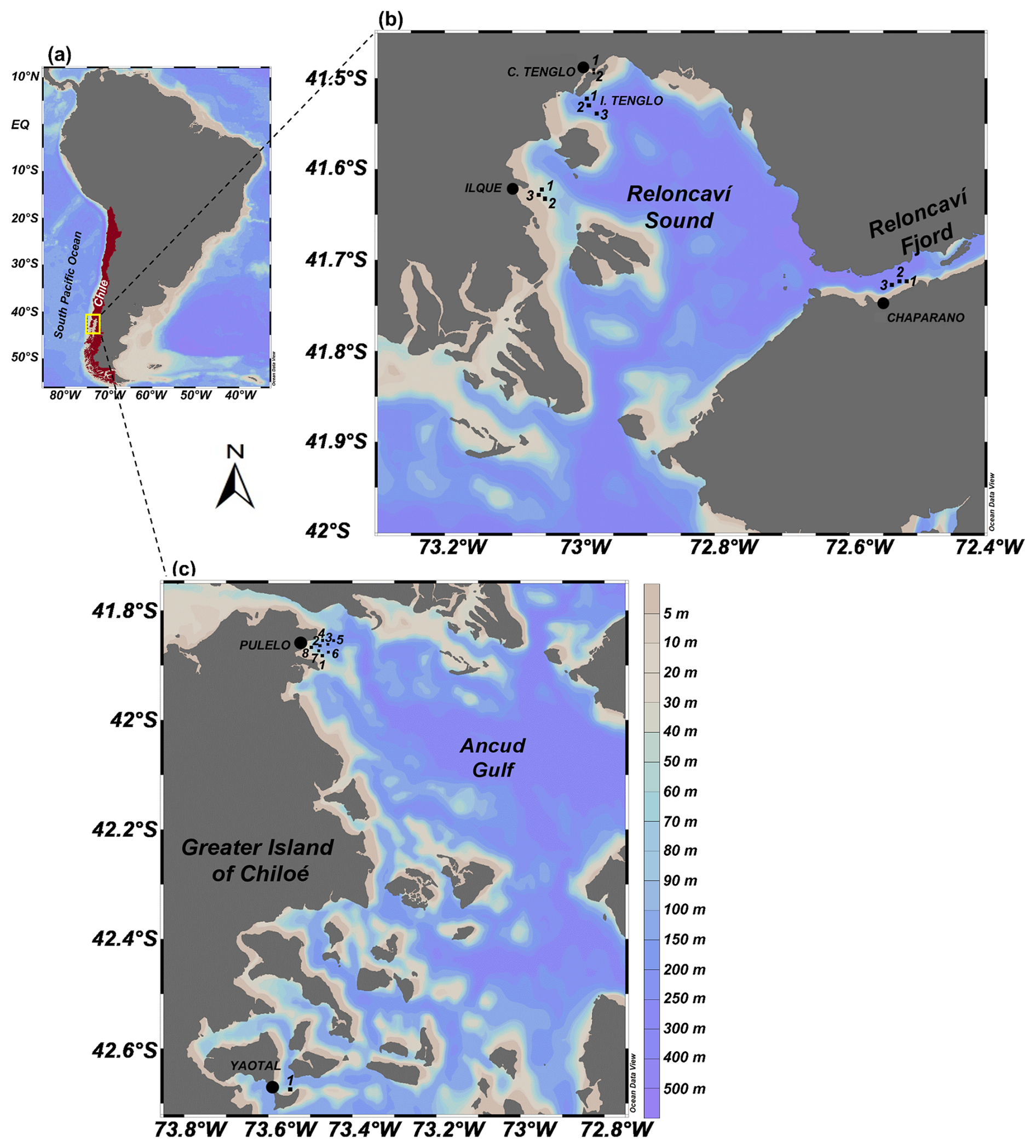
Figure 1 (a) Study area in the northern Patagonian fjords of Chile (∼41.45–42.75° S) (yellow box), and sampling locations at (b) Reloncaví Sound and (c) Greater Island of Chiloé.

Throughout this complex coastal system, freshwater inputs from rivers, rainfall, groundwater and melting glaciers generate an estuarine circulation pattern (Dávila et al., 2002; Valle-Levinson, 2010; Castillo et al., 2016), which has a considerable influence over the biogeochemical processes and physical oceanography in the area. The freshwater inputs generate stratification conditions which strongly impact the bio-optical water properties and support the growth of diatom-dominant phytoplankton communities (Iriarte et al., 2007; Silva et al., 2011; González et al., 2019).

2.2 Field sampling

The present study implemented a field sampling strategy from January to May 2023 (the summer-autumn period in the southern hemisphere) in the coastal system that constitutes the area of study in order to acquire in situ hyperspectral images and oceanographic data pertaining to temperature, salinity and phytoplankton.

Specific sectors were selected for the in situ sampling from across the study area (Fig. 1) based on a set of criteria, including historical physical-chemical characteristics (temperature, salinity and turbidity), local circulation patterns, HAB occurrence and proximity to aquaculture facilities (Table S1 in the Supplement) (Silva et al., 2011; Soto et al., 2019, 2021).

Six locations were identified throughout the area in line with the aforementioned criteria. These were: Ilque (I), Isla Tenglo (T) and Canal Tenglo (CT), all within the Reloncaví Sound coastal system; Chaparano (C), located in the Reloncaví Fjord; and Pulelo (P) and Yaotal (Y), two sampling points located on the coast of the Greater Island of Chiloé (Table S1, Fig. 1b and c). Sampling transects of three or four stations were performed across these monitoring locations, depending on topography and UAV flight autonomy.

The field sampling was undertaken during daylight hours (∼ 10:30–16:00 LT – local time) under safe and optimal weather conditions. Although meteorological conditions varied between clear and cloudy days, all sampling transects were conducted under conditions in which there was no rain, wind speeds were low (<15 m s⁻¹) and surface waters were calm (waves < 1 m).

Water samples for oceanographic monitoring were collected simultaneously with the optical data at each station. The geo-location (latitude/longitude) was sent from equipment onboard the research ship to the UAV technician, who was located on the shore, to coordinate water sampling using aerial observations. The autonomous flights were configured using DJI Pilot 2 drone software at an altitude of 100 m above the sea surface and a flight speed of ∼1–2 m s⁻¹, in order to obtain images of an area of 2500 m² around the oceanographic sampling points.

Since phytoplankton is commonly distributed within the first ∼20–30 m of the water column, two sampling depths were established: the first was at the surface (∼1.5 m), while the second was based on water transparency rather than at a defined depth. Temperature, salinity and in situ chlorophyll a (Chl a) levels were established using two conductivity, temperature and depth probes (CTDs), an RBRconcerto³ and an AML-Oceanographic Metrec XL. Transparency was determined by a Secchi disk. Water samples were collected using a Niskin bottle, at both the surface and at Secchi depths, and stored in opaque plastic bottles for subsequent analysis at the laboratory, in terms of both phytoplankton in situ total biomass (Chl a) and phytoplankton abundance and taxonomy. Discrete water samples collected for analyses of phytoplankton abundance and taxonomy were fixed with Lugol's iodine solution (1 %).

2.3 Phytoplankton analysis

Phytoplankton species abundance was estimated according to the microphytoplankton range (∼20–200 µm) in the laboratory. The phytoplankton identification and cell counts were performed following the Utermöhl method (Utermöhl, 1958), i.e., 10 mL of a fixed water sample were sedimented from day to day prior to observations being taken using an inverted light microscope (Olympus CKX-41). Taxonomic identification was conducted to the lowest rank possible (genus or species) (Mardones and Clément, 2016).

2.4 UAV system, reflectance measurement and hyperspectral imaging

The UAV deployed in the present study was a DJI Matrice 300 RTK drone with the capacity to support a maximum weight of ∼9 kg and a flight autonomy of approximately 30 minutes (Fig. 2a). A hyperspectral camera, model Resonon Pika L, was connected to the drone by a custom-made 3D printed carbon fibre gimbal (Fig. 2b). In addition, an Intel NUC mini-personal computer (mini-PC) was attached to the drone using a custom-made 3D printed mount, including batteries (Fig. 2b).

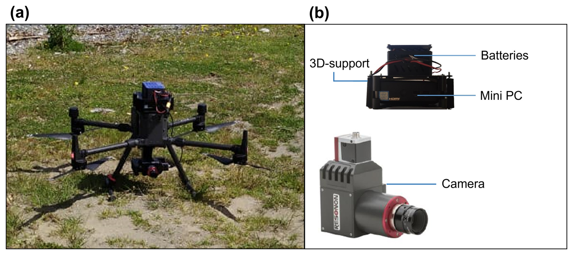
Figure 2 UAV system: (a) DJI Matrice 300 RTK drone, and (b) Resonon Pika L hyperspectral camera, 3D printed mount with batteries and Intel NUC mini-PC.

The Resonon Pika L camera captures 236 spectral bands covering a spectrum range from ∼400 to 900 nm with a spectral resolution of approximately ∼2.1 nm. A Flame S spectrometer (Flame Ocean Insight) was used to record the light conditions (solar radiation) during the flight, in the same spectral bands as those captured by the hyperspectral camera. A laptop connected via a cellular connection or a Wireless Local Area Network (WLAN) to the mini-PC was used to operate the camera and record reflectance data. In remote areas where connectivity was not available, communication between computers was established by an Ubiquiti Loco M5 access point through a local wireless network.

2.5 Data processing and analyses

Prior to conducting the data analyses, a pre-selection was performed, in which all samples with several co-occurring phytoplankton genera (>3) were removed from the final dataset. Only stations where one or a maximum of two genera dominated the community by >80 % of abundance were considered for the reflectance fingerprint analysis and differentiation among the spectral signals.

Several steps were involved in processing the raw image data captured by the hyperspectral camera using Spectronon Pro software. The raw data were processed to obtain reflectance (R(λ)) using the calibration file provided by Resonon and the downwelling irradiance data provided by a miniature spectrometer (Flame Ocean Insight). Subsequently, pixel cleaning was undertaken using an adapted Normalized Difference Water Index (NDWI), whereby pixels that did not correspond to water and those that were saturated due to the solar angle of incidence were masked (Xie et al., 2014). Due to the lack of reference points in the monitoring areas, non-geometric correction was applied to the raw image data. A consequence of this was that the raw data were used only as reflectance data rather than images in the present study. These data were normalized using the min-max method. The Savitzky–Golay method, or digital smoothing polynomial filtering (DISPO), based on the least-squares polynomial smoothing and differentiation fit (Ruffin and King, 1999; Gallagher, 2020), was then applied to reduce the noise signal and obtain a clean spectrum, without altering its properties. Finally, reflectance data were averaged in order to obtain a reflectance value at each band to emphasize the shape singularities of each spectrum. For analysing and comparing the spectral signals of the different phytoplankton species, the reflectance R(λ) values were used at a spectral resolution of approximately ∼2.1 nm, while the wavelength bands were limited to the visible and near-infrared light of between 400 and 750 nm.

A hierarchical cluster analysis (HCA) was performed to explore the changes in R(λ) under different genera domains. A resemblance matrix based on the hyperspectral normalized R(λ) was generated using the nearest neighbour single linkage algorithm and the cosine index, as a distance measure for calculating similarities among spectral signals. Differentiation among spectral signals for the stations in which the same phytoplankton genus domain was identified using the non-parametric Kolmogorov–Smirnov test. To assess the influence of pigment concentration at spectral signals, a statistical analysis was applied to determine the differences among low (<2 µg L⁻¹), moderate (>4 µg L⁻¹) and high (>8 µg L⁻¹) Chl a concentrations.

The in situ temperature and salinity were converted to the conservative temperature and absolute salinity by applying the algorithms proposed in the Thermodynamic Equation of Seawater 2010 (TEOS-10). The conservative temperature is similar to the potential temperature, although it represents the heat content of seawater with greater precision. Conversely, absolute salinity represents the spatial variation in the composition of seawater by considering the different thermodynamic properties and the horizontal density gradient in the open ocean (IOC et al., 2010). Oceanographic variables across the present study area were characterized on a seasonal scale, with a permutational analysis of variance (One-way PERMANOVA) conducted to determine the differences between the stations. Prior to the analysis, data were homogenized (log-transformed) and normalized in order to enhance approximate multivariate normality.

Data were visualized and processed using Ocean Data View (ODV) (Schlitzer, 2023), in which the Data-Interpolating Variational Analysis (DIVA) for gridding and interpolation were applied (Troupin et al., 2012), and also by PRIMER 7 (Clarke and Gorley, 2015) and PAST 4.06 software tools (Hammer et al., 2001).

3 Results

3.1 Phytoplankton and spectral signals

Although the phytoplankton community identified in the present investigation was typical of the summer-autumn diatoms assemblage described for the area of study, its composition changed between seasons, with an increase in diversity and a decrease in dominance, in addition to a slight increase in richness in the autumn, with the exception of Canal Tenglo (Fig. 3, Table S2).

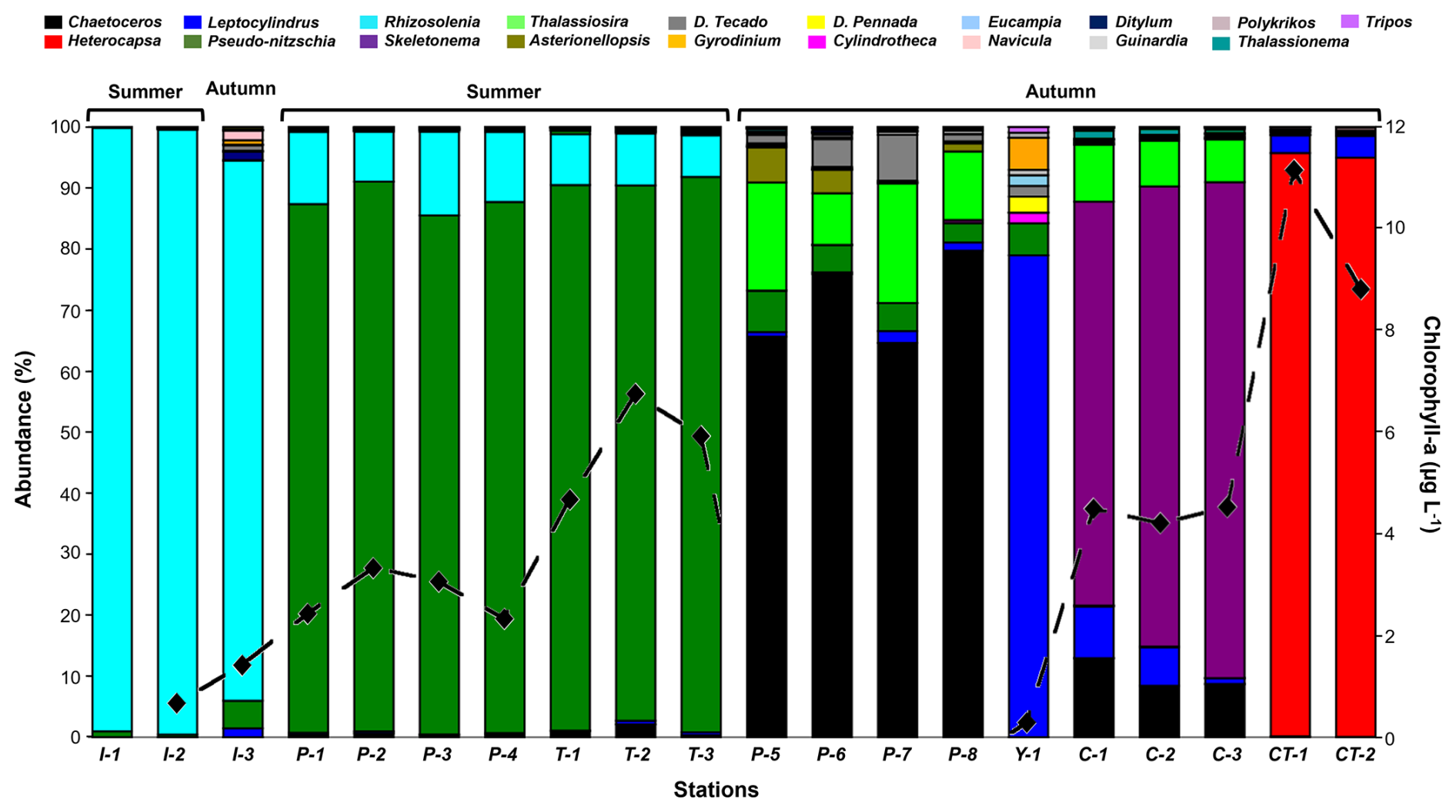
Figure 3 Microphytoplankton community composition (histogram) and total biomass (black dotted line) during summer and autumn at sampling locations. Each colour represents a genus of the community. Location codes: I = Ilque, P = Pulelo, T = Isla Tenglo, Y = Yaotal, C = Chaparano, and CT = Canal Tenglo.

Although merely one bloom of the microalgae Heterocapsa triquetra was detected during the study period, composition analysis showed a clear monogenus domain (>80 % abundance) of Rhizosolenia sp. at Ilque, and Pseudo-nitzschia sp. at Pulelo and Isla Tenglo, in the summer (Fig. 3). In the autumn, a combination of two genera was required in order to reach 80 % abundance, at Chaparano, Yaotal and Pulelo (Fig. 3).

Although the reflectance spectrums, under a diatom genus domain, displayed similar patterns across the blue and green bands (∼400–565 nm), differences in the shape of the curve and the reflectance values were observed, including between sample stations at the same location (Figs. 4 and 5). During summer, samples at Ilque, which were dominated by Rhizosolenia sp., displayed significant differences in the spectral signal (p<0.01) between stations in both the blue (∼400–490 nm) and the green to near infra-red (∼500–750 nm) bands (Fig. 4a, Table S3).

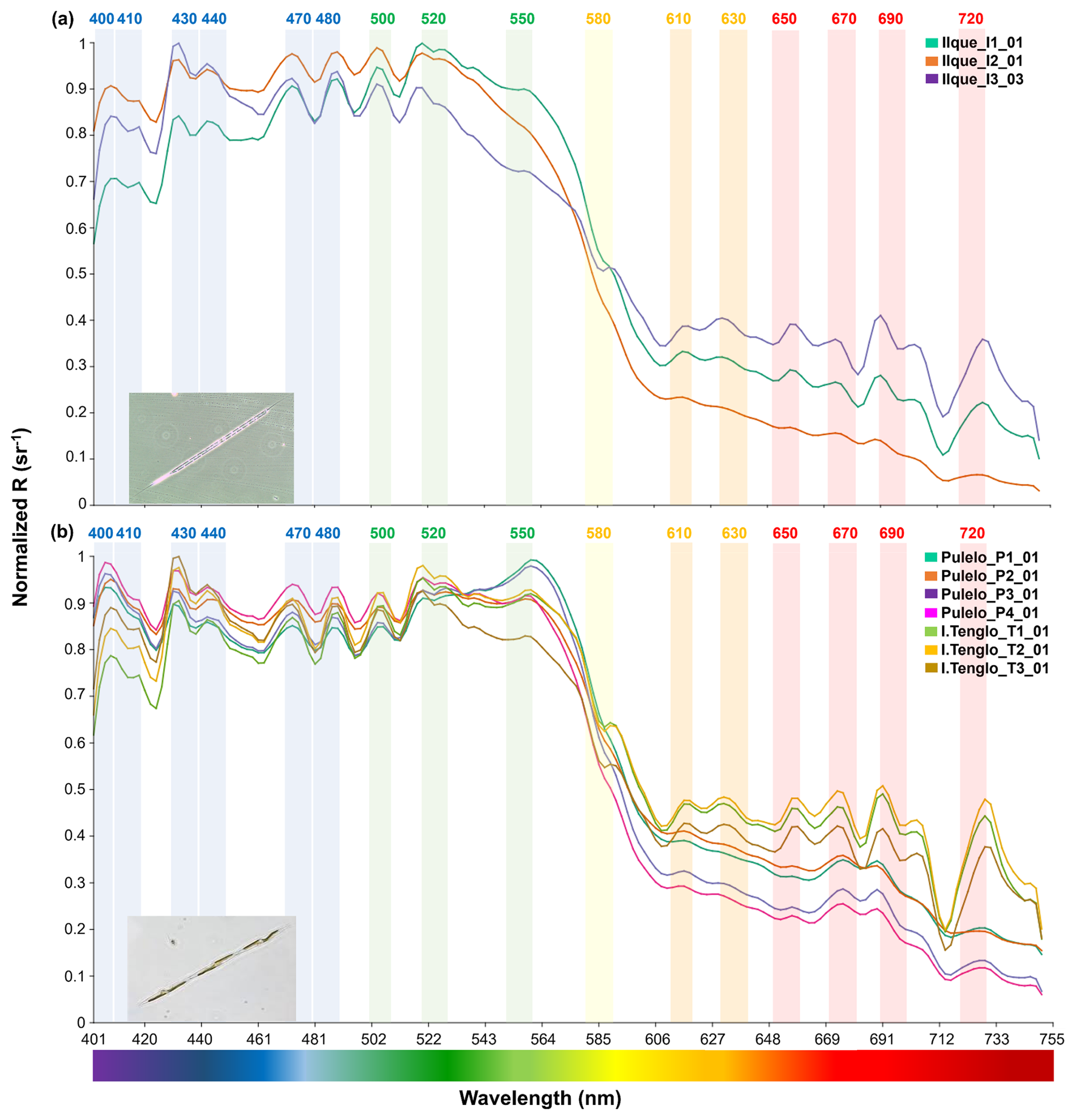
Figure 4 Diatoms spectral signals: (a) Rhizosolenia sp. at Ilque (aqua green, orange and purple lines); (b) Pseudo-nitzschia sp. at Pulelo (aqua green, orange, purple and pink line) and Isla Tenglo (jasmine green, yellow and brown line) (∼41.45–42.75° S).

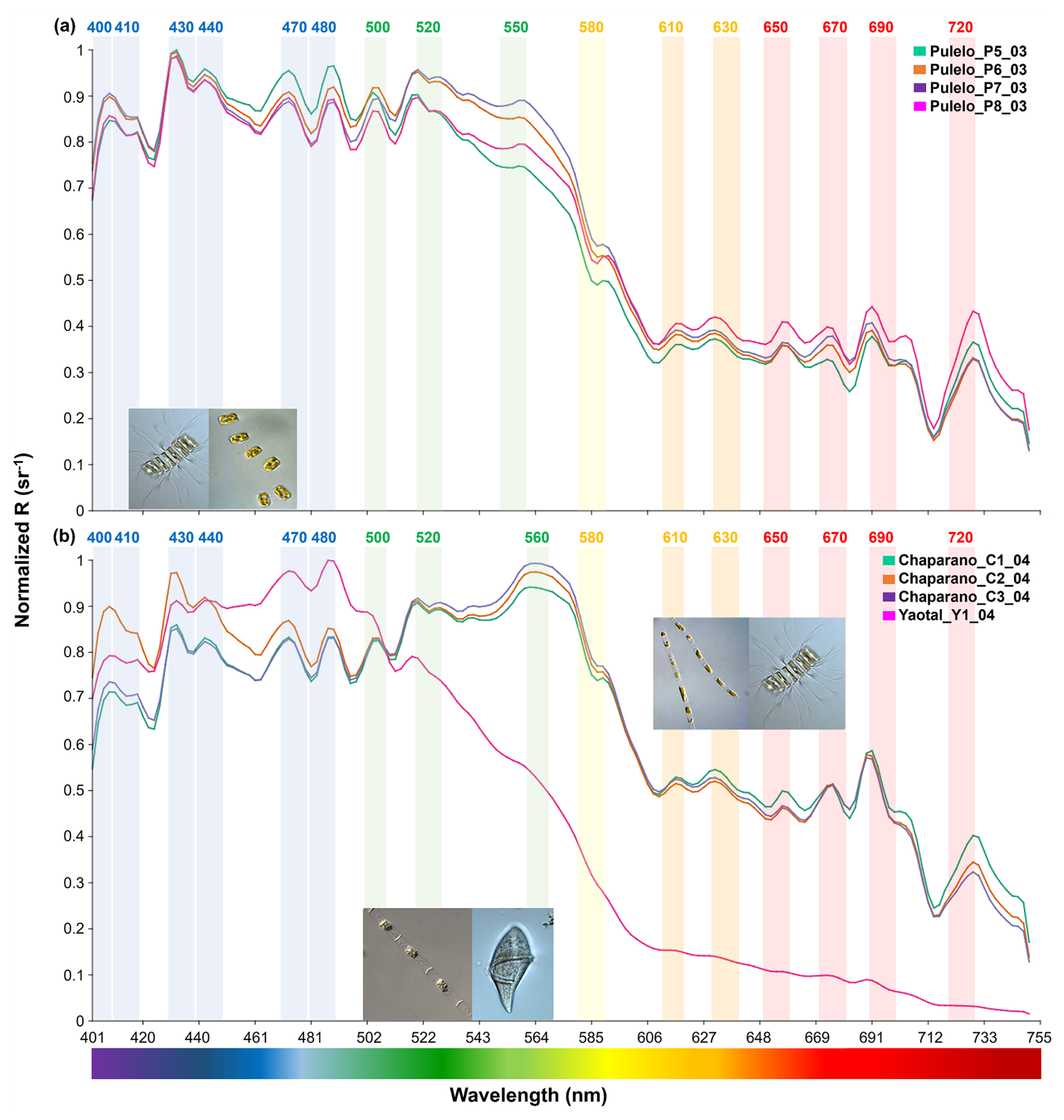
Figure 5 Diatoms spectral signals: (a) Chaetoceros sp. and Thalassiosira sp. at Pulelo (green, orange, purple and pink lines); (b) Skeletonema sp. and Chaetoceros sp. at Chaparano (green, orange and purple lines) and Leptocylindrus sp. and Gyrodinium sp. at Yaotal (pink line) (∼41.45–42.75° S).

Similarly, under Pseudo-nitzschia sp. domain, significant spectral differences (p<0.01) were detected at Pulelo in the total spectrum (Table S3). In the blue (∼400–490 nm) bands, similar signals recorded at stations 1 and 3 differ from those measured at stations 2 and 4 (Fig. 4b, Table S3). In the same way, signals from stations 1 and 2 differed significantly in the spectral signal from those at stations 3 and 4 (Fig. 4b, Table S3), from the green to near infra-red (∼500–750 nm) bands. At Isla Tenglo, only station 3 displayed a spectral signal significantly different in the green to near infra-red (∼500–750 nm) bands (Fig. 4b, Table S3).

The analysis displayed a more homogeneous reflectance signal in relation to the March to April (autumn) samples (Fig. 5). At Pulelo, similar spectral signals were detected, with the exception of station 8 (Fig. 5a, pink line), in the green to near infra-red (∼500–750 nm) bands (Fig. 5a, Table S3). Furthermore, only station 2 at Chaparano (Fig. 5b, orange line) displayed a statistically different total spectrum (p<0.05) and spectral signal in the blue (∼400–490 nm) bands (p<0.01) (Fig. 5b, Table S3).

By performing a band-based comparison, it was found that all samples under diatoms genera domain displayed a similar pattern in the blue (∼400–490 nm) bands, with the exception of Leptocylindrus sp. at Yaotal, with the highest R(λ) (>0.9 sr⁻¹) registered at 470–480 nm (Fig. 5b). In the green (∼500–565 nm) bands, where chlorophyll pigments reflect light, generally high values of reflectance (>0.9 sr⁻¹) were recorded, in addition to a higher variability in terms of both shape and R(λ) values (Figs. 4 and 5). In fact, at Ilque, where Rhizosolenia sp. dominated, the reflectance exhibited an acute downward slope between the green and yellow (∼550–610 nm) bands (Fig. 4a), in which the absorption peaks of accessory pigments, such as phycoerythrin and phycocyanin, are usually detected. A similar slope was observed at Pulelo and Isla Tenglo under Pseudo-nitzschia sp. domain (Fig. 4b). This slope was less pronounced at Chaparano (Fig. 5b).

The spectral reflectance from all diatom genera displayed a declining slope in the red to near-infra-red (∼650–740 nm) bands, where another peak in chlorophyll reflectance is typical. In this area of the spectrum, two main peaks were observed, between ∼680–720 nm and with an acute decline at ∼714 nm (Figs. 4 and 5). Strong variability was registered among genera in this area of the spectrum, with the highest values detected at Chaparano for the Skeletonema sp. and Chaetoceros sp. assemblage (Fig. 5b).

Furthermore, important differences were observed in the spectra between diatoms and dinoflagellates. The spectral signal of dinoflagellates was captured on merely one occasion, under a bloom of the Heterocapsa triquetra species. The spectrum shape of this species displayed a completely different pattern compared to those of diatom genera. In the Heterocapsa triquetra spectral signal, a clear increase in the R(λ) from the blue to green bands (∼400–565 nm) was observed (Fig. 6).

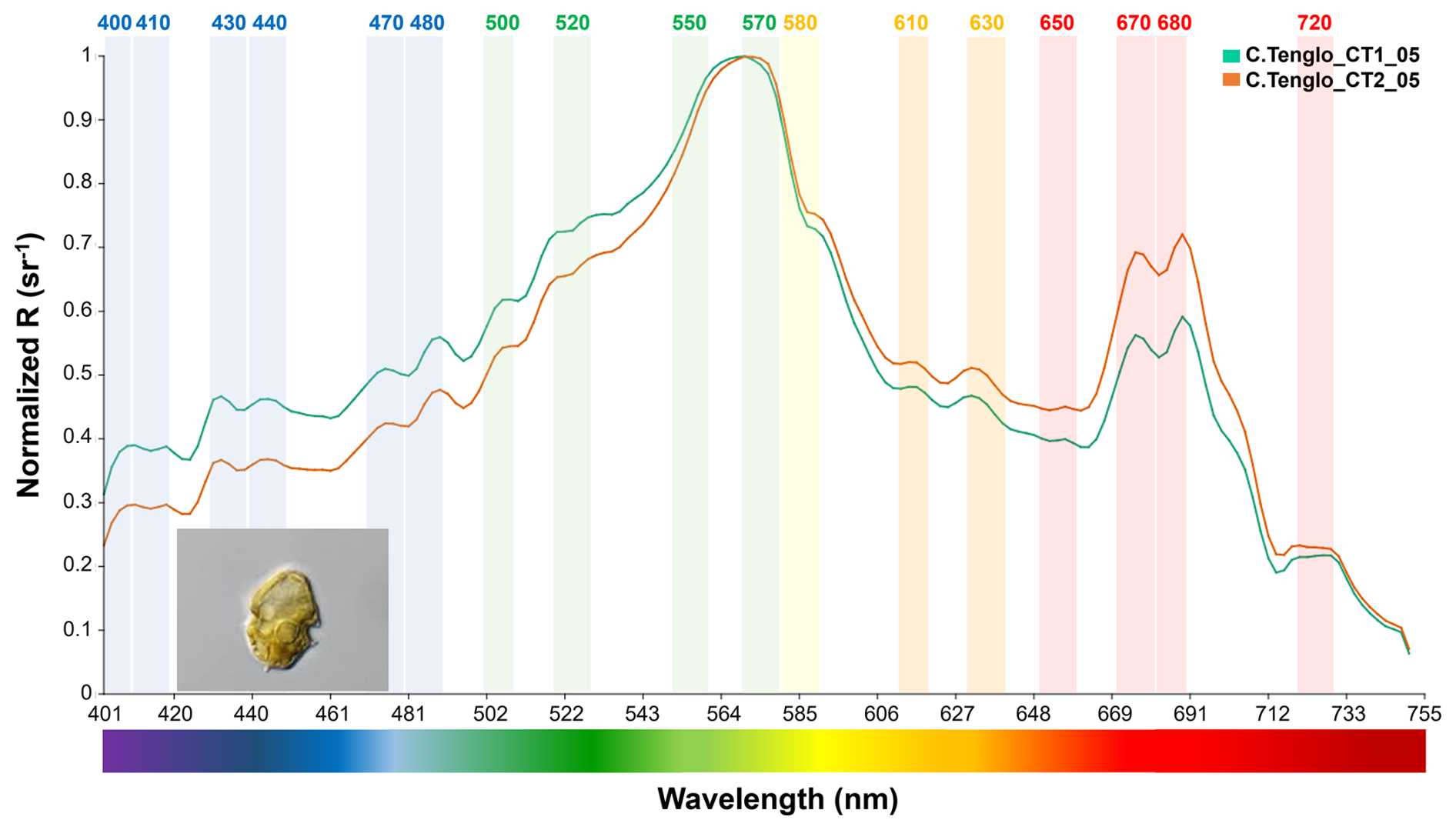
Figure 6 Spectral signal of the dinoflagellate Heterocapsa triquetra at Canal Tenglo (green-Sta.1, orange-Sta.2) (∼41.45–42.75° S).

R(λ) values were up to two or three times lower than for diatoms in the blue (∼400–490 nm) bands (Figs. 4–6), with differences observed between station signals (Table S3). The main peak of R(λ) was at 570 nm in the yellow-green area (Fig. 6). Differences between dinoflagellates and diatoms were also registered in the red to near infra-red (∼650–740 nm) bands, with a distinctive signal of two R(λ) peaks at 670 and 680 nm (>0.55 sr⁻¹), in conjunction with a plateau structure at 720 nm (Figs. 4–6). In summary, differences between groups were detected by means of the shape (Figs. 4–6), the peaks observed at 440, 470, 500, 520, 550, 570 and 580 nm, and the variations in magnitude displayed in the blue-green (∼400–565 nm) and the red to near infra-red (∼650–740 nm) bands (Figs. 4–6).

3.2 Oceanographic conditions and reflectance

Oceanographic conditions were subject to seasonal changes (F=8.18, p<0.01), whereby the highest conservative temperature was registered in the summer of 2023, while conservative temperatures generally ranged from 14–18 °C (Fig. 7a and b). In the autumn, the water temperature reduced overall variability, with maximum values not exceeding 13 °C in the surface layer (Fig. 7c and d).

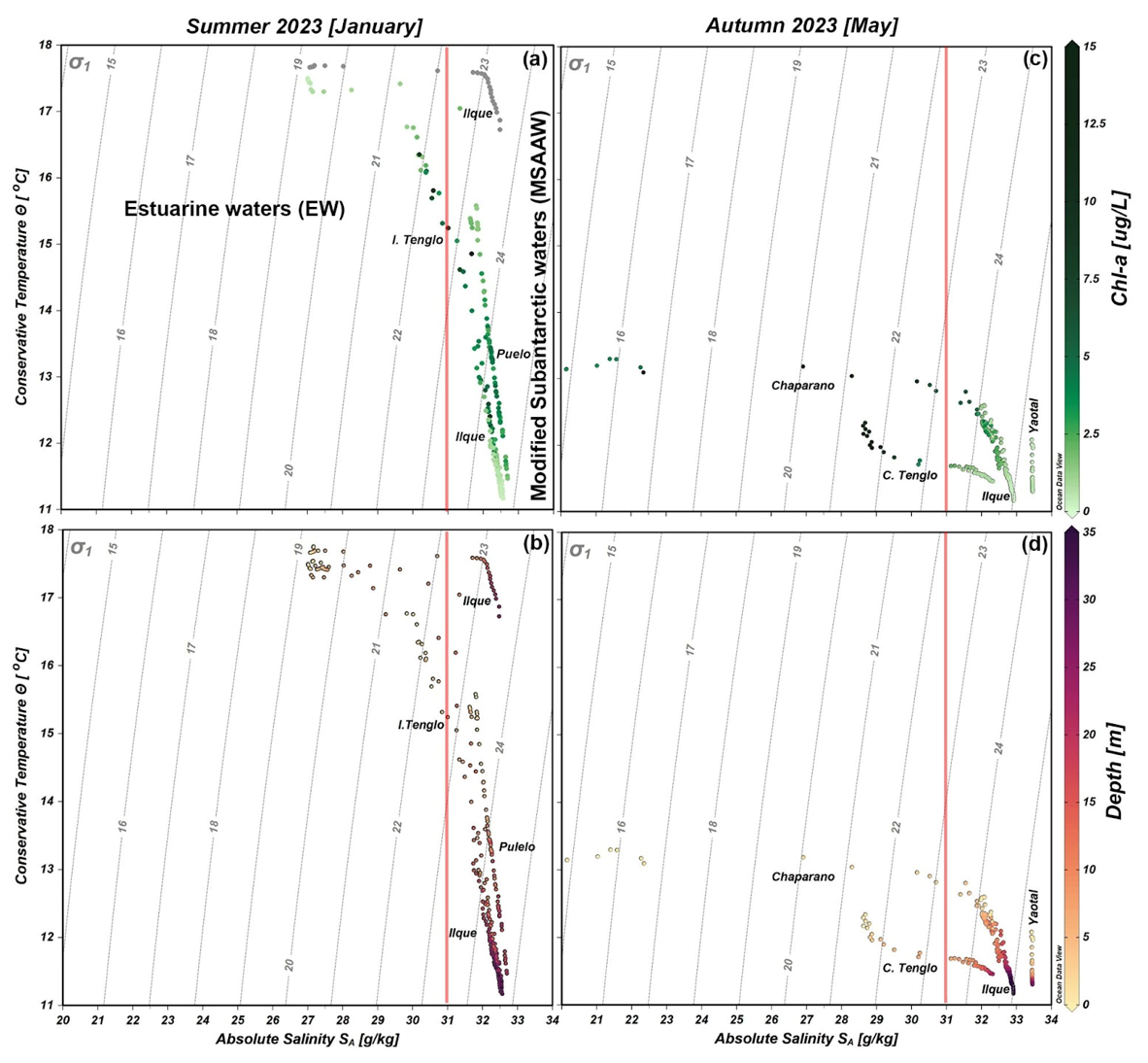
Figure 7 Conservative temperature and absolute salinity scatter diagram, including density (σ) isoline (grey vertical lines) collected during the 2023 summer and autumn oceanographic campaigns. Images (a) and (c) show incorporation of Chl a; images (b) and (d) show water depth where data was obtained. In (a) the grey dots in the Ilque area denote no Chl a data.

The absolute salinity minimum was observed in the surface layer (20–22 g kg⁻¹) of Chaparano during the autumn, contributing to the decrease in water density (Fig. 7d). In summer, absolute salinity varied from 26–33 g kg⁻¹ (Fig. 7b). According to the salinity criteria (Sievers and Silva, 2008), estuarine water (0–31 g kg⁻¹) and modified subantarctic water (31–33 g kg⁻¹) were observed along both seasonal stations. In the case of Chl a distribution, the highest values (15 µg L⁻¹) were registered at the surface layer of Canal Tenglo during the autumn, although no general pattern was observed.

In terms of chlorophyll a, the reflectance spectra displayed variability when different Chl a concentrations were compared (Fig. 8). For example, significant differences (p<0.01) in spectra signals were detected at Ilque, with Rhizosolenia dominant, between January (low Chl a = 0.8 µg L⁻¹) and March (high Chl a = 1.6 µg L⁻¹).

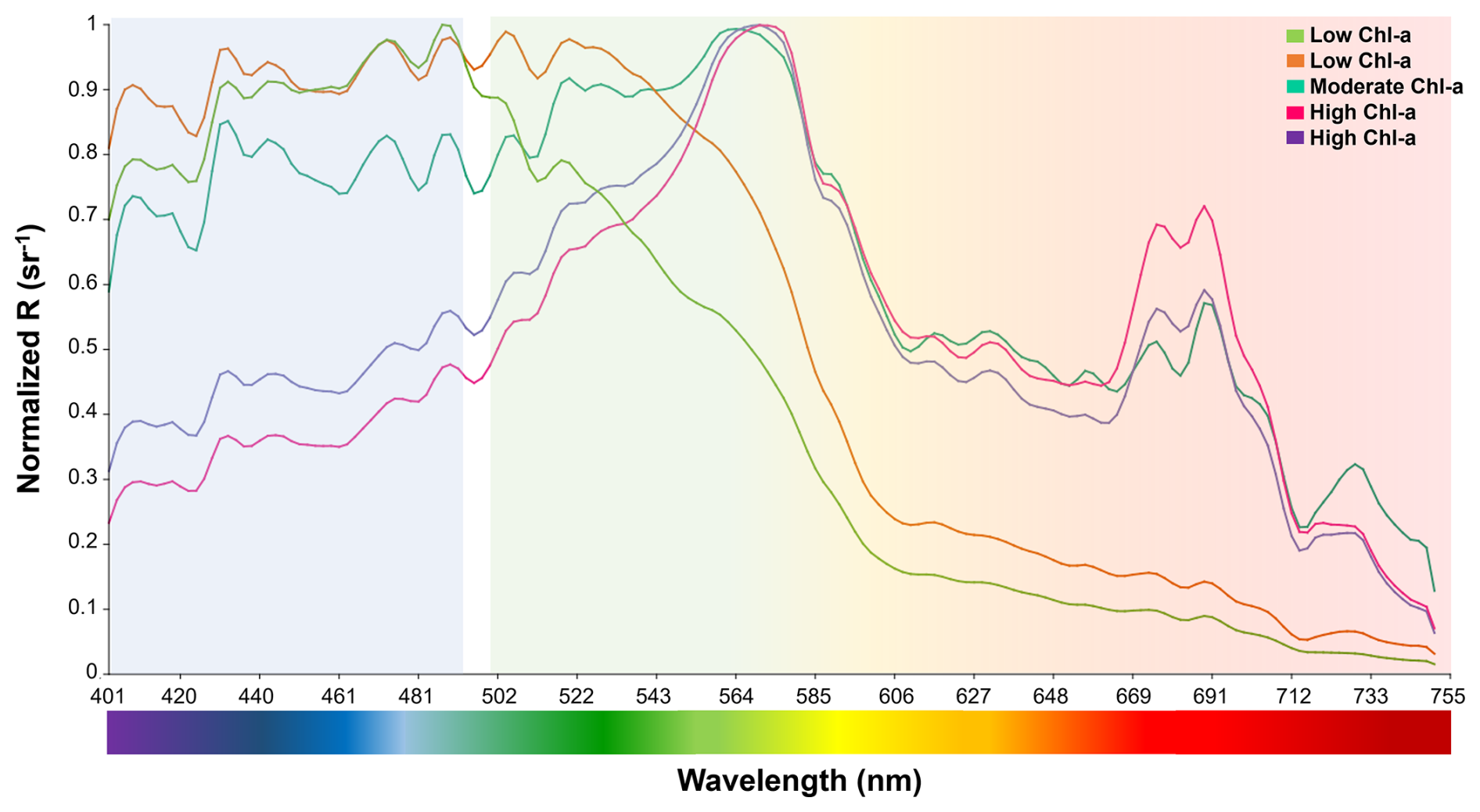
Figure 8 Microphytoplankton spectral signals with different Chlorophyll a concentrations. Low chlorophyll a (<2 µg L⁻¹) (jasmine green and orange lines); moderate chlorophyll a (>4 to 7.9 µg L⁻¹) (aqua green line); and high chlorophyll a (>8 µg L⁻¹) (pink and purple lines).

Also in January, measurements at Pulelo (low Chl a = 2.92 µg L⁻¹) and Isla Tenglo (high Chl a = 5.93 µg L⁻¹) exhibited significant differences (p<0.01), with Pseudo-nitzschia dominant. Regardless of the dominant species, at low Chl a concentration levels (<2 µg L⁻¹) reflectance spectral signals exhibited more significant variability in the green-red (from 500 to 750 nm) bands, while under moderate (>4 µg L⁻¹) to high (>8 µg L⁻¹) Chl a concentrations this variability was greater in the blue (∼400–490 nm) band (Fig. 8).

Finally, the cluster analysis grouped together spectra that corresponded to stations under the same dominant groups and genera more closely (Fig. 9). Although similarity values were high, two main distinctions were identified: the first relates to locations being grouped together due to the dominance of diatoms, while the second relates to locations grouped together due to the dominance of the dinoflagellate Heterocapsa triquetra (Canal Tenglo) (Fig. 9).

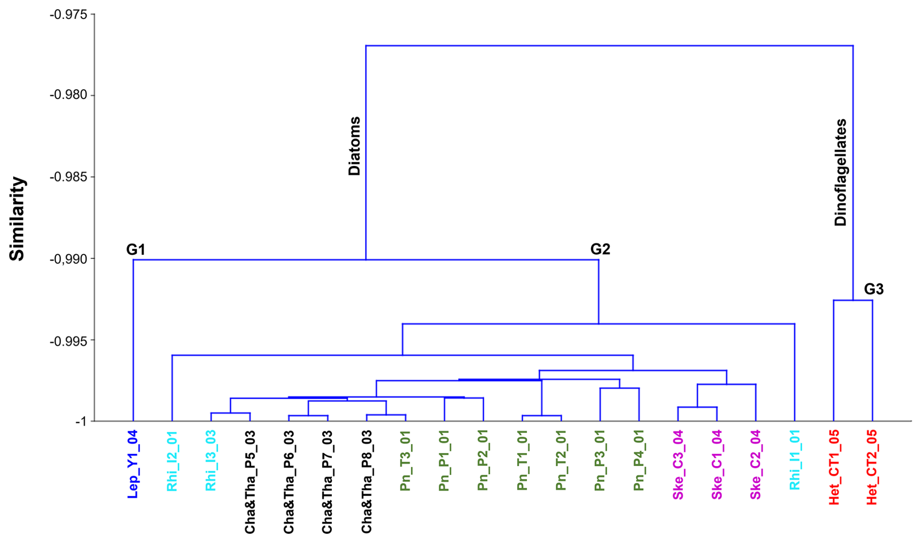
Figure 9 Dendrogram of microphytoplankton hyperspectral normalized R(λ) signals classified by the dominant genus. Colours identify different genus and sampling locations: Leptocylindrus sp. in Yaotal (blue); Rhizosolenia sp. in Ilque (cyan); Chaetoceros sp. and Thalassiosira sp. in Pulelo (black); Pseudo-nitzschia sp. in Pulelo and Isla Tenglo (green); Skeletonema sp. in Chaparano (violet) and Heterocapsa triquetra in Canal Tenglo (red).

Within the diatoms, two groups can be described. The first (G-1) pertains to the group identified at Yaotal during the autumn, which was dominated by Leptocylindrus sp. (78.95 %), in which the dinoflagellate Gyrodinium sp. (5.26 %) was the secondary genus. The second group (G-2) grouped together the remaining locations that were dominated by diatoms (Fig. 8). Within G-2, all samples were grouped together by the dominant genus, with the exception of Ilque (Fig. 9). Nevertheless, the dendrogram grouped together locations based not only on the dominant genus, but also on the basis of similar oceanographic conditions (Fig. 9). Thus, when observing Fig. 9 it is possible to see Yaotal (blue) and Ilque (cyan) on the left side of the cluster, which were associated with changes in salinity during the autumn season and characterized by low Chl a values. On the right side of the cluster, the locations of Canal Tenglo (red) and Chaparano (violet) were characterized by the detection of high Chl a values.

4 Discussion

4.1 Phytoplankton assemblages and spectral R(λ) variability

In the present work, a hyperspectral R(λ) data set with a total of 20 R(λ) spectra was obtained. This data set characterizes the fingerprints of the main phytoplankton groups as well as the predominant genera in the northern Patagonian fjords (Iriarte et al., 2007; Alves-de-Souza et al., 2008; Jacob et al., 2014; Cuevas et al., 2019). These spectral fingerprints are representative of the most dominant species-genera among the phytoplankton community and appear consistent, including under varying oceanographic conditions. The results of the present paper are highly relevant, particularly in a context in which a limited number of existing datasets or studies incorporate in situ hyperspectral reflectance (R(λ)) as a new means with which to investigate phytoplankton composition (Casey et al., 2020).

In the present study, two main groups (diatoms and dinoflagellates) and three sub-groups of phytoplankton assemblages were identified through the R(λ) spectrum, with a variability observed not only between groups, but also among genera. Although the R(λ) spectrum of different diatom genera was similar in shape and magnitude across the blue to green bands (∼400–520 nm), the spectral signal enabled the “fingerprints” of different genera to be detected. These differences are especially observed at the blue (∼400–490 nm) and the red to near infra-red bands (∼650–740 nm), where the absorption and fluorescence of accessory pigments are highest (Kramer et al., 2022).

In the red to near infra-red bands (∼650–740 nm), absorbance peaks of 683 and 700 nm have been previously related to HABs (Shen et al., 2012), in concurrence with the drops in reflectance values registered for both diatom and dinoflagellate groups in the present study. Past spectral studies have shown differences in the signal of diatoms and dinoflagellate species (Tao et al., 2013). For example, Zhao et al. (2010) described three different spectral fingerprints that grouped several species together. In the aforementioned study, the dinoflagellate Heterosigma akashiwo was characterized by a single reflectance peak of 680–750 nm. However, the results of the present study showed a more accurate spectrum, due to the width of the spectral signal, with a double peak structure between 670–690 nm, a plateau at around 720–730 nm and a previous higher peak in the green bands at ∼570 nm. This main peak has been previously described to characterize the spectral signal of the HAB dinoflagellate species Lepidodinium chlorophorum (Gernez et al., 2023), thus raising the possibility of it being considered a dinoflagellate spectral signal characteristic. However, the hyperspectral reflectance results of diatom species in the present study demonstrate a similar peak at around 560–570 nm for Skeletonema sp., in line with studies that utilize satellite remote-sensing reflectance (Tao et al., 2013).

The effects of pigment concentrations and the community composition of phytoplankton on the reflectance spectrum have been shown to be essential factors in the development of optical fingerprints at the genus or species levels (Mao et al., 2010; Kramer et al., 2022; Gernez et al., 2023). Although increases in absorbance and decreases in reflectance generally correlate directly with changes in algal density (cell concentration) in monospecific laboratory experiments (Gitelson et al., 1999), non-significant differences in spectral signals under different cell concentrations were detected during field monitoring. The lack of relationship between cell density and reflectance is likely given in the range of densities observed in the present study, which varied from 1 582 600 to 3400 cells per litre. In this context, the main factor that affects reflectance signals with differences in curve shapes in relation to the same species was related to pigment concentration (Chl a). In fact, significant differences in major spectral bands (blue, green and red) were observed on the basis of this pigment concentration. In the summer, under low Chl a concentrations, peaks in reflectance in the green-red (∼500–750 nm) bands, where chlorophyll pigment reflects light, showed significant variability in both shape and magnitude of R(λ), both among genera and across the different locations. In terms of spectral signals registered in the autumn, under higher Chl a concentrations and a more diverse community, greater variability was detected in the blue (∼400–490 nm) bands. However, as indicated by Mao et al. (2010), such variations in the blue bands (i.e., 400–450 nm) are driven by the species composition under low Chl a concentrations, in contrast to the green (500–550 nm) bands.

Recent studies have described a covariation between pigments, both accessory and specific groups, and optical properties such as fluorescence, scattering or cellular grouping (Kramer et al., 2022). In the present study, total Chl a has been shown to play a key role in the spectra with the R(λ) signal classification. The HCA groups together the same phytoplankton assemblages and genera, including under variable oceanographic conditions (primarily by salinity and Chl a). Furthermore, it groups locations with similar total biomass concentration (Chl a) and phytoplankton community composition. Locations with open water circulation, in which there were different dominant diatoms genera, characterized by low total biomass concentrations (min. <1 µg L⁻¹), higher salinity and the presence of dinoflagellates (Gyrodinium sp. and other thecate dinoflagellates) were grouped together more closely (Yaotal, Ilque and Pulelo). Conversely, stations with high Chl a concentrations (min. >1 µg L⁻¹), located mainly in enclosed areas like Chaparano and Canal Tenglo, formed part of another group. Additionally, it should be noted that locations with the lowest Chl a concentrations also displayed the lowest mean values of abundance.

The variability in reflectance can be associated with multiple factors, including biological (community composition, cellular morphology, cell density, pigment composition and concentration or physiological status), physical-chemical (suspended matter, stratification, the roughness of the surface or the specular reflection), and meteorological (wind speed, solar radiation, cloudiness and solar angle) (Gitelson et al., 1999; Kim et al., 2016; Muñoz et al., 2023). For example, stratification plays a key role in the vertical distribution of phytoplankton and matter in estuarine and coastal waters. River discharge and glacier melting constitute an important input of coloured dissolved organic matter (CDOM) and total suspended matter (TSM), and they also alter the bio-optical signals, especially in the blue bands (Simis et al., 2017; Kramer et al., 2022; Adhikari et al., 2023). Indeed, in the Patagonian fjords, and particularly in the Chiloé Inner Sea, high synchrony between Chl a and turbid river plumes has been detected using remote sensing reflectance (Rrs₆₄₅ product) at 645 nm (Muñoz et al., 2023).

In fact, variations in bio-optical water properties have not only been related to a punctual parameter, but also to the interactions of these parameters and their seasonality (Flores et al., 2022; Adhikari et al., 2023; Muñoz et al., 2023), with changes in the optical signal associated with both biological (phytoplankton succession) and non-biological (stratification) characteristics in the water column (Simis et al., 2017). Moreover, the ability to accurately distinguish the effect of different factors on in situ reflectance signals is complex, since it may be a nonlinear relationship. Therefore, further research is necessary to understand both the biological features, i.e., phytoplankton composition and pigment concentration, including accessory pigments, and non-biological characteristic on the reflectance signal.

4.2 New technologies: limitations, opportunities and challenges

Optical technology for the remote detection of phytoplankton, such as satellites, have been employed for decades (Hu et al., 2005; Shen et al., 2012; Moisan et al., 2017; Gernez et al., 2023). Although limitations related to satellite observations associated with spatial-temporal and spectral band resolution are well known (Muller-Karger et al., 2018; Schaeffer and Myer, 2020), more modern satellites that use multi- or hyperspectral sensors, such as Plankton, Aerosol, Cloud, Ocean Ecosystem (PACE) and Hyperspectral Imager for the Coastal Ocean (HICO), have shown improvements in spatial (∼1200–90 m) and/or spectral resolution (∼350–900 nm) in recent years (Kramer et al., 2022; Gernez et al., 2023). Crucially, these modern multi- or hyperspectral sensors favour observation in the ultraviolet (UV), visible and near-infrared bands. Nevertheless, certain limitations remain in terms of the number of spectral bands and satellite orbit cycles or those caused by cloud cover and sunglint in remote areas.

Accurate observations represent a challenge in coastal areas where the spatial-temporal variability of phytoplankton changes rapidly. The recent development of new technologies, such as UAVs and hyperspectral cameras to detect and monitor phytoplankton blooms, particularly harmful algae species at a high spatial-temporal resolution, can fill in the gaps of satellite data and also help to validate this data with in situ measurements. The utility of this technology in terms of in situ measurements has been demonstrated around the world, especially in coastal areas in which current or future economic activities, or future projects under prospecting are present (Kim et al., 2016; Kimura et al., 2019; McEliece et al., 2020; Min et al., 2021). Consequently, an essential factor in this regard is the optical system chosen for to capture the spectral signal. Currently, there are multiple possibilities, including radiometers and hyperspectral and multispectral cameras, which offer several characteristics, such as distinct spectral resolutions, different model sizes and varying imaging systems (Kislik et al., 2018; Olivetti et al., 2023). Although hyperspectral cameras are a high-cost technology, their high resolution is considered the best option for phytoplankton and HAB monitoring in complex and small coastal areas with aquaculture activities, including fjords, bays and estuaries (Olivetti et al., 2023).

The present study has identified a series of advantages and challenges of using UAVs and hyperspectral technology for the detection and identification of phytoplankton assemblages in complex coastal waters. One of these advantages is the continuous spectral resolution afforded by the hyperspectral camera, which is capable of measuring each ∼2 nm, from 400 to 1000 nm, i.e., it is a powerful tool with which to differentiate between phytoplankton assemblages through changes in spectral signals at high spectral resolution. The use of UAVs for in situ reflectance measurement is another advantage. For example, conducting monitoring at optimal altitudes (<100 m) allows for a high spatial resolution (∼3.5 cm by pixel) to be achieved. UAVs can also be deployed to capture reflectance under cloud cover or other atmospheric conditions, such as suspended dust and other particulate matter. These advantages contrast with the major challenges in terms of capturing satellite reflectance in coastal systems with complex topographies and high cloud cover throughout the year. The challenge is especially significant if it is necessary to obtain images and water samples simultaneously.

Despite the aforementioned advantages, the use of UAVs as a means of phytoplankton monitoring in remote areas remains a challenge. Although this technology can help to reduce sampling times and provide researchers with the possibility to conduct monitoring in remote coastal areas, the dependency on a strong network signal in the vicinity constitutes a major limitation, particularly in more isolated areas where network signal is weak or inconsistent. Furthermore, adverse weather conditions, such as wind or rain, as previously identified by Kislik et al. (2018), can compromise the use of a UAV. Other limitations that were identified during the undertaking of the present study relate to technical aspects, including flight time being limited by battery life and the lack of reference points over large expanses of water (Kislik et al., 2018; Wu et al., 2019). A further aspect to consider is the camera size. Hyperspectral cameras are a relatively new technology and, as such, are large and heavy. Therefore, their functionality is somewhat limited since those who wish to utilize this equipment are forced to invest in a large, expensive drone in order to carry the camera. In addition, a further related challenge to overcome is the high variability of these cameras available on the market, with a broad range of specifications in terms of spectral resolution, geometry acquisition and imaging systems. As a result, a degree of caution is required at the moment of acquisition because the specifications of the camera that is purchased will determine the ability of the user to capture and compare data and apply algorithms in future work. Further significant obstacles that can hinder the identification of phytoplankton using reflectance data include the analysis of the vertical distribution of phytoplankton in the water column (∼1–40 m), using both satellites and UAV-hyperspectral camera systems, particularly in the design of future algorithms. This also includes the difficulties associated with conducting analyses of the presence of other particles, mainly non-biological, in the water column, as well as their impact on solar radiation absorption/reflexion and in terms of other physical aspects, such as water roughness.

The high resolution afforded by this new technology has the potential to enhance the classical detection algorithms that are based on reflectance and/or absorbance ratios and which have traditionally been applied on the basis of satellite data (Mao et al., 2010; Tao et al., 2013; Gernez et al., 2023). However, despite recent works having increasingly included hyperspectral data for the study of phytoplankton assemblages, these datasets remain limited to specific areas and/or are unavailable. Indeed, the lack of a robust hyperspectral image library is another important factor to consider. Therefore, future observations must combine UAV-hyperspectral camera systems and next-generation satellite hyperspectral data with the in-situ collection of biological (phytoplankton concentration, pigments and taxonomy) and non-biological data (CDOM and TSM) across multiple and diverse environments.

5 Conclusions

The aim of the present study was to take the first steps in the identification of phytoplankton from in situ hyperspectral signals using a UAV and hyperspectral technology in a complex coastal system, which in this case was the Patagonian fjords. The results obtained show the potential of hyperspectral data for the detection and identification of phytoplankton assemblages. Evidence was found of differences between the spectral signals of diatoms (i.e., Rhizosolenia sp., Pseudo-nitzschia sp. and Leptocylindrus sp.) that were detected in the blue band (∼400–490 nm) with those of dinoflagellates (i.e., Heterocapsa triquetra) that were observed in the red to near-red bands (∼650–740 nm), regardless of cellular concentration. In addition, pigment concentrations were validated as determinants, with Chl a playing a significant role in the classification of the reflectance spectra signal. The present study illustrates the great potential of hyperspectral technology and the usefulness of UAV systems to support and improve both satellite and in situ monitoring in complex coastal waters, such as the Patagonian fjords. The reflectance data registered in the present study, which is associated with a specific genera label, in conjunction with information on oceanographic conditions and phytoplankton pigments, can be employed in a possible next step to aid in the development of an accurate algorithm through machine learning. This would not only help to identify and differentiate phytoplankton genera blooms, but also non-biological particles (suspended materials and sediment) and other water characteristics.