Contribution of meridional overturning circulation and sea ice changes to large-scale temperature asymmetries in CMIP6 overshoot scenarios

This work analyzes overshoot simulations from 13 models, including the SSP5-3.4OS and SSP1-1.9 experiments from the Coupled Model Intercomparison Project Phase 6 (CMIP6), to assess how regional temperatures after overshoot differ from those of before, and how these differences may be impacted by changes in sea ice, the Atlantic Ocean Heat Transport (OHT) and the Atlantic Meridional Overturning Circulation (AMOC). The overshoot scenarios, characterized by a peak in radiative forcing levels followed by a decline, show that changes during the CO₂ increasing phase are not necessarily compensated during the CO₂ decreasing phase, particularly at the regional level. Even if the global mean temperature may recover after the overshoot, regional conditions post-overshoot may still differ from those pre-overshoot, with spatial patterns characterized by large-scale temperature asymmetries. These asymmetries are found between Northern (NH) and Southern Hemisphere (SH), between high and mid-latitudes of the NH, and between western and eastern areas of the Southern Ocean. Changes in sea ice and ocean circulation are identified as potential sources of hysteresis, highlighting the impact of oceanic changes in the behavior of atmospheric variables in case of overshoot. The analyses from this work show that the relative contribution of each mechanism strongly depends on the model. Inter-model differences in the contributions of the meridional overturning can be associated with different climatologies of Mixed Layer Depth (MLD) in the northern North Atlantic (NNA) and in certain areas of the Southern Ocean. Despite these differences across models, both ocean circulation and sea ice changes contribute to shaping the regional temperatures after overshoot, with the temperature asymmetries between NH and SH mainly explained by changes in the AMOC, those between high and mid-latitudes of the NH by sea ice changes, and those between western and eastern areas of the Southern Ocean by the Southern Meridional Overturning Circulation (SMOC). These results highlight the importance of model intercomparison and analysis of ocean dynamics to understand the regional impacts of an overshoot, and more generally the responses to forcing changes.

1 Introduction

The growing probability of exceeding the temperature targets of the Paris Agreement of 2015 (Raftery et al., 2017), as a result of delays in implementing effective mitigation measures (IPCC, 2022), increases the likelihood of overshoot scenarios. In these scenarios, global average temperature surpasses the target of 1.5 °C above pre-industrial levels (United Nations/Framework Convention on Climate Change, 2015) and is reduced to the target afterwards with net-negative emissions (Gasser et al., 2015). However, large uncertainties exist for these possible scenarios, including the feasibility of recovering pre-overshoot temperatures with large-scale Carbon Dioxide Removal (CDR) in the expected timescales, and the long-term climate risks associated with reinforced Earth-system feedbacks characteristic of such scenarios (Schleussner et al., 2024).

Considering the increasing interest in these overshoots, the Coupled Model Intercomparison Project Phase 6 (CMIP6; Eyring et al., 2016) included in the ScenarioMIP (O'Neill et al., 2016) two scenarios with Shared Socio-economic Pathways (SSP) that reach a peak before starting a forcing decline: SSP5-3.4OS and SSP1-1.9. Both of these represent Overshoot Scenarios (OS), but at different forcing levels. While SSP1-1.9 includes mitigation actions to meet the 1.5 °C target of the Paris Agreement with a moderate overshoot, SSP5-3.4OS follows the unmitigated scenario SSP5-8.5 up to 2040 and starts an aggressive mitigation afterwards (Tebaldi et al., 2021).

The analysis of these scenarios shows different behaviors for global and regional climates. Even if global temperatures revert, the impact on regional temperature, precipitation and climate extremes may remain for decades (Pfleiderer et al., 2024). This regional irreversibility, understood as a post-overshoot state different from the pre-overshoot state with the same CO₂ concentration levels and with the same global temperature, is associated with hemispheric temperature asymmetries between pre-overshoot and post-overshoot states (Roldán-Gómez et al., 2025), impacting the precipitation of tropical areas through changes in the position of the Intertropical Convergence Zone (ITCZ). These temperature asymmetries may be linked to persistent changes in the Ocean Heat Transport (OHT) and to different thermal inertia depending on the region (Roldán-Gómez et al., 2025), but also to other factors like anthropogenic aerosol emissions (England et al., 2021) and ice melting (Li et al., 2020).

The analysis of the SSP1-1.9 and SSP5-3.4OS scenarios confirms the relevant role of hysteresis mechanisms in shaping regional temperature and precipitation after global temperature overshoots. Hysteresis is understood as the dependence of the climate system not only on the current CO₂ concentration but on the CO₂ pathway. Relevant hysteresis mechanisms are found in the large-scale hydrology, with persistent changes in global precipitation after a CO₂ overshoot (Cao et al., 2011), with changes in the position of the ITCZ associated with a delayed energy exchange between the tropics and extratropics (Kug et al., 2022), and with impacts on the monsoon system, with a contrasting eastern-western hemispheric monsoon response in the NH (Oh et al., 2022) and an enhanced El Niño-like warming pattern altering the East Asian summer monsoon (Song et al., 2022).

Hysteresis is also found in ocean dynamics and sea level changes (Palter et al., 2018), in Antarctic ice sheet retreat (Garbe et al., 2020; Bochow et al., 2023), in ocean acidification (Jiang et al., 2024) and in ocean carbon cycle feedbacks (Schwinger and Tjiputra, 2018). Li et al. (2024) show that the post-overshoot state in SSP5-3.4OS is characterized by a persistent weakening of Atlantic Meridional Overturning Circulation (AMOC), with impacts on the OHT also for the Southern Ocean and, to a lesser extent, for the Indo-Pacific basin. However, there are large uncertainties in these changes, with responses of the AMOC to forcing changes that strongly depend on the model considered (Sgubin et al., 2017; Bellomo et al., 2021). In global warming conditions, a decrease in OHT is generally found (Mecking and Drijfhout, 2023), both in the NH and in the SH, but models disagree on the presence of tipping points, with only some models showing a local convection collapse in the subpolar North Atlantic, and only a few of them presenting a full AMOC disruption (Sgubin et al., 2017). Changes in the AMOC also depend on the emission scenario and the associated loss of sea ice (van Westen and Baatsen, 2025). A collapse of the AMOC may have important impacts at a global scale (Orihuela-Pinto et al., 2022), stressing the need to understand in which conditions it may occur (Jackson et al., 2023). Baker et al. (2025) show that the collapse of the AMOC is unlikely even under extreme forcing conditions, and may only occur in case a strong Pacific Meridional Overturning Circulation (PMOC) emerges.

This work analyzes overshoot scenarios from CMIP6 (SSP5-3.4OS and SSP1-1.9) to better understand why models present a different level of irreversibility in ocean dynamics and sea ice changes, and how this translates into the emergence of different large-scale temperature asymmetries in the post-overshoot climate. Asymmetries between Northern (NH) and Southern Hemisphere (SH), between high and mid-latitudes of the NH, and between western and eastern areas of the Southern Ocean are correlated with changes in the OHT, including contributions of the AMOC in the Atlantic basin and of the Southern Meridional Overturning Circulation (SMOC) in the Southern Ocean, as well as with changes in the ice cover in both the NH and SH. These analyses, covering the entire range of responses present in CMIP6 models, allow for a complete assessment of the relative contribution of each mechanism to temperature asymmetries, and for a better understanding of the different responses found in regional climates after the overshoot.

2 Methods

The analyses are based on all the available simulations of CMIP6 overshoot experiments SSP5-3.4OS and SSP1-1.9, listed in Table 1. This includes 165 simulations from 11 different models for SSP1-1.9, all of them covering the period from 1850 to 2100, and 16 simulations from eight models for SSP5-3.4OS, with four of them covering an extended period from 1850 to 2300. As shown in Table 1, ensembles of simulations with the same forcing specifications and different initial conditions are available for some of the models, including CanESM5 and UKESM1-0-LL for SSP5-3.4OS, and CanESM5, MIROC6, MIROC-ES2L, IPSL-CM6A-LR, EC-Earth3, MPI-ESM1-2-LR, MRI-ESM2-0, and UKESM1-0-LL for SSP1-1.9. The use of ensemble averages allows to better separate the responses to forcing changes from potential contributions of internal variability. In addition to the ensemble of simulations from each individual model, combined ensembles are also considered, including the ensemble of all simulations (ALL) for SSP1-1.9 and SSP5-3.4OS, and the ensemble of simulations covering the extended period (EXT) for SSP5-3.4OS. Considering the disparity in the number of simulations available for each model (only one SSP1-1.9 simulation for CNRM-ESM2-1, FGOALS-g3 and GFDL-ESM4, and up to 50 SSP1-1.9 simulations for CanESM5 and MIROC6), the use of the same weight for each simulation would generate an ensemble average mostly driven by a few models with large ensembles. To avoid that, the ensemble averages of the ALL and EXT ensembles are computed by averaging all the simulations from each model to obtain a per-model average in a first step and by averaging all the models in a second step, so that all the models contribute with the same weight to the multi-model average. The ALL ensemble of SSP5-3.4OS contains 16 simulations from 8 models, covering the period from from 1850 to 2100, while the EXT ensemble of SSP5-3.4OS contains only 4 simulations from 4 models, but covering an extended period from 1850 to 2300. Both ensembles are then complementary, being the ALL ensemble mostly used to analyze the inter-model dispersion and the EXT ensemble mostly used to analyze the long-term stabilization after the overshoot. For MRI-ESM2-0, CNRM-ESM2-1 and IPSL-CM6A-LR the only available SSP5-3.4OS simulation covers the extended period, so there is no difference between the extended simulation and the ensemble average. However, for CanESM5 there is one simulation covering the extended period and 4 simulations covering only from 1850 to 2100. In that case, the extended simulation is identified as CanESM5-EXT, while the average of the 5 simulations is identified as CanESM5.

Ziehn et al. (2021)Swart et al. (2019a, b)Lovato et al. (2021)Voldoire (2019a, b)Döscher et al. (2022); EC-Earth-Consortium (2019a, b, c)Li (2019, 2020)John et al. (2018)Boucher et al. (2019a, b)Shiogama et al. (2019)Tachiiri et al. (2019)Schupfner et al. (2021)Yukimoto et al. (2019a, b)Good et al. (2019a, b)

Table 1 Models and simulations considered in this work, resolution of atmospheric (ResA) and ocean component (ResO) of each model and associated references. For the SSP5-3.4OS, the simulations covering the extended period (up to 2300) are included in the column (EXT).

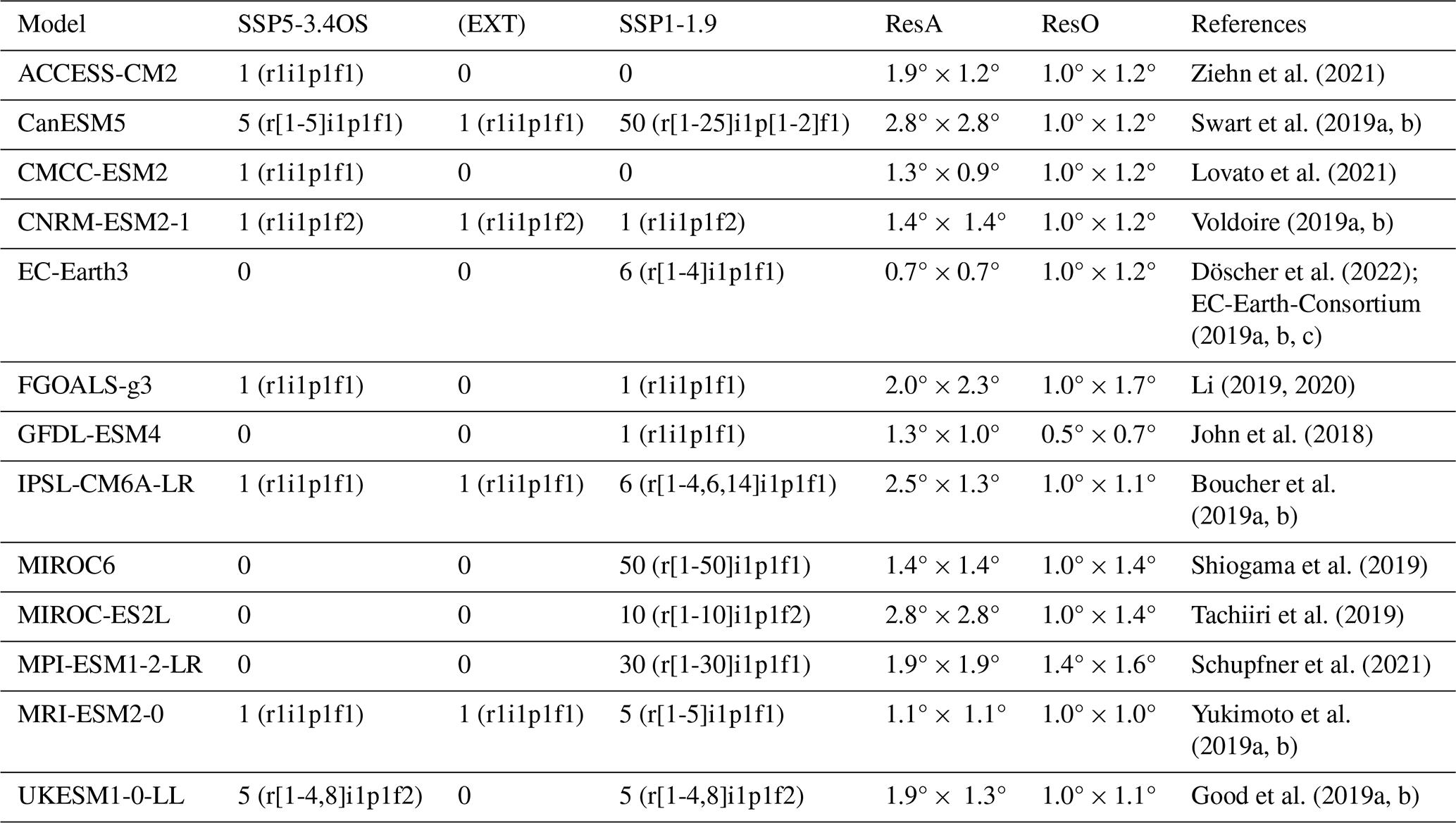
As shown in Table 1, the resolution of the atmospheric component of the selected models varies from 2.8 to 0.7°, while the resolution of the ocean component varies from 1.7 to 0.5°. To allow for combined analyses, a longitude-latitude grid is considered both for the atmospheric and the ocean variables, and all the simulations are remapped with a bilinear interpolation to a common grid resolution of 2.8°, the coarsest among the analyzed climate models.

In a first step, analyses are focused on annual Sea Surface Temperatures (SST), to characterize the temperature asymmetries generated during the overshoot. For that, the temporal evolution of SST and the difference between pre- and post-overshoot states are analyzed, considering all the ocean basins. To highlight the long-term variability, the temporal evolutions are filtered with a 10 year moving average. The post-overshoot state is defined as a 20-year period from 2220 to 2239 for SSP5-3.4OS EXT and from 2080 to 2099 for the SSP1-1.9 and the SSP5-3.4OS ALL ensemble. This post-overshoot state is compared with the pre-overshoot state with the same global average of surface air temperature, which is reached in 2034 for SSP5-3.4OS and in 2030 for SSP1-1.9, and the pre-overshoot state with the same CO₂ concentration (Meinshausen et al., 2020), reached in 2015 both for SSP5-3.4OS and SSP1-1.9. Considering these dates and in order to use a reference period large enough to focus on the long-term variability, our pre-overshoot reference for all analyses (except those stated otherwise) is the period from 2020 to 2039. Despite their secondary role with respect to changes in CO₂ concentration, potential differences in aerosol emissions between SSP5-3.4OS and SSP1-1.9 are assessed by considering the aerosol emissions provided by Feng et al. (2020).

To evaluate temperature asymmetries between pre- and post-overshoot states, and considering the results from Roldán-Gómez et al. (2025), the regions included in Fig. 1 are considered. In particular, the asymmetry between NH and SH is characterized as the difference between regional averages of SST for the extratropical ocean areas of the NH (EN) and the extratropical ocean areas of the SH (ES), the asymmetry between mid and high latitudes of the NH is characterized with the difference between regional averages for mid-latitude extratropical ocean areas of the NH (ENM) and high-latitude extratropical ocean areas of the NH (ENH), and the asymmetry between western and eastern areas of the Southern Ocean is characterized with the difference between regional averages for south-western Southern Ocean (SSW) and south-eastern Southern Ocean (SSE). The asymmetries have been evaluated for all the basins together, considering the results from Roldán-Gómez et al. (2025) and the existing connections between Atlantic, Southern Ocean and Indo-Pacific basins (Li et al., 2024). To confirm that the results are not sensitive to this choice, results for EN, ES and ENM but including only the Atlantic basin (ENATL, ESATL and ENMATL) are included in Appendix A.

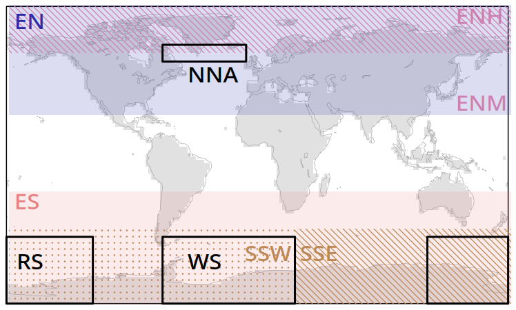
Figure 1 Regions considered for the analysis of temperature asymmetries and MLD, including extratropical ocean areas of the NH (EN; 23–90° N), high-latitude extratropical ocean areas of the NH (ENH; 60–90° N), mid-latitude extratropical ocean areas of the NH (ENM; 23–60° N), extratropical ocean areas of the SH (ES; 90–23° S), south-western Southern Ocean (SSW; 90–45° S; 180° W–25° E), south-eastern Southern Ocean (SSE; 90–45° S; 25–180° E), northern North Atlantic (NNA; 55–65° N; 70–10° W), Weddell Sea (WS; 90–50° S; 70° W–25° E), and Ross Sea (RS; 90–50° S; 120° E–120° W).

In a second step, some mechanisms and processes potentially contributing to these temperature asymmetries are explored. Considering the large model differences existing for these variables (Sgubin et al., 2017), the analyses are focused on the global, Atlantic and Pacific OHT, the Atlantic mass transport, the sea ice concentration, and the Mixed Layer Depth (MLD) provided by the models. A set of indices are defined to evaluate their variability, including the Atlantic OHT at 26° N, the global OHT at 50° S, the total sea ice area for the NH and the SH, the average March MLD for the northern North Atlantic (NNA, as defined in Fig. 1), and the average September MLD for Weddell Sea and Ross Sea (WS and RS, as defined in Fig. 1). The difference between pre- and post-overshoot states and the temporal evolution of these indices are evaluated for each simulation of SSP5-3.4OS and SSP1-1.9 experiments, as well as for the ensemble average of each individual model and the average of ALL and EXT ensembles.

3 Results

3.1 Temperature asymmetries

The evolution of the global average of SST for the SSP5-3.4OS and SSP1-1.9 experiments is shown in Fig. 2a and b. At the end of the simulations (2300 for the extended simulations of SSP5-3.4OS and 2100 for the others), the global average of SST for the SSP5-3.4OS EXT ensemble (gray line in Fig. 2a) and the SSP1-1.9 ALL ensemble (red line in Fig. 2b) is larger than that of the situation before the overshoot with the same global average of surface air temperature (horizontal solid line; reached in 2034 for SSP5-3.4OS and in 2030 for SSP1-1.9) or the situation before the overshoot with the same CO₂ concentration (horizontal dashed line; reached in 2015 both for SSP5-3.4OS and SSP1-1.9). This shows that the heat accumulated by the ocean during the CO₂ increasing phase is not totally released to the atmosphere afterwards, in line with the results from Roldán-Gómez et al. (2025). Despite this common result for the EXT and ALL ensembles, strong differences exist across the simulations and models. For example, for the extended simulation of MRI-ESM2-0 in SSP5-3.4OS (gold line in Fig. 2a) and for the ensemble average of MIROC6 (brown line in Fig. 2b), MIROC-ES2L (orange line in Fig. 2b), MPI-ESM1-2-LR (dark grey line in Fig. 2b), and MRI-ESM2-0 (gold line in Fig. 2b) in SSP1-1.9, the global average of SST after overshoot is lower than that of before.

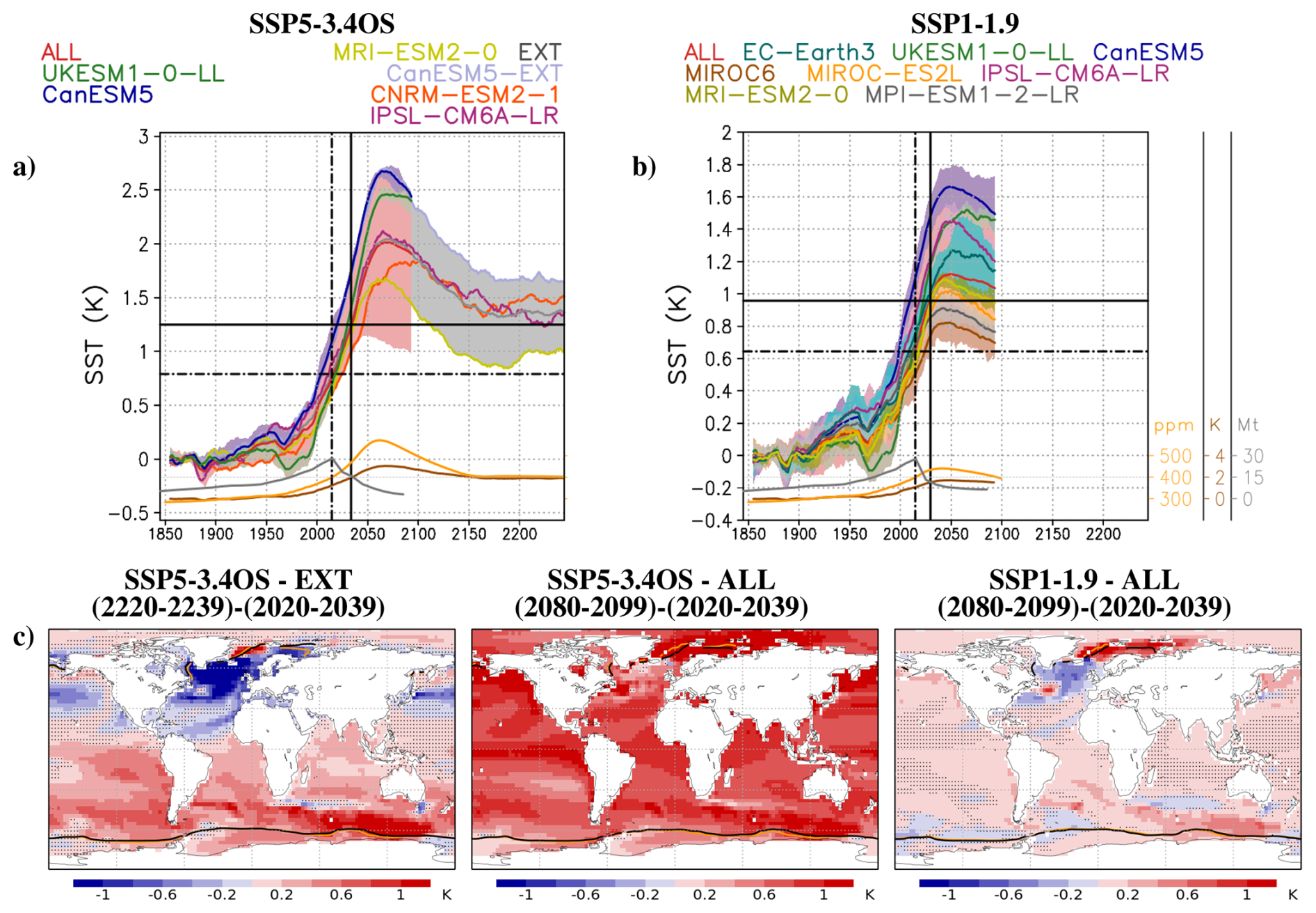
Figure 2 (a, b) Global average of Sea Surface Temperature (SST) anomaly with respect to 1861–1880 obtained from the CMIP6 simulations of experiments (a) SSP5-3.4OS and (b) SSP1-1.9, including the ALL and EXT ensembles, the ensemble average for each individual model and the individual extended simulations. Envelopes show the min-max values within each ensemble. Yellow, gray and brown curves in the lower part of each panel respectively show the CO₂ concentration from Meinshausen et al. (2020), the anthropogenic aerosol emissions from Feng et al. (2020), and the global surface air temperature obtained with the SSP1-1.9 ALL ensemble and the SSP5-3.4OS EXT ensemble. The vertical lines show the year before the overshoot with the same CO₂ concentration (dashed line) and global surface air temperature (solid line) as at the end of the run (2100 for the SSP1-1.9 ALL ensemble and 2300 for the SSP5-3.4OS EXT ensemble), while the horizontal lines represent the value of SST in the SSP1-1.9 ALL ensemble and in the SSP5-3.4OS EXT ensemble for those years. (c) Difference between the ensemble mean, temporal average values of SST for (left) the periods 2220–2239 and 2020–2039 obtained with the SSP5-3.4OS EXT ensemble, (center) the periods 2080–2099 and 2020–2039 obtained with the SSP5-3.4OS ALL ensemble, and (right) the periods 2080–2099 and 2020–2039 obtained with the SSP1-1.9 ALL ensemble. Contours of 15 % of sea ice concentration are included in the maps, both for the periods 2220–2239 and 2080–2099 (yellow) and for the reference period 2020–2039 (black). Stippling indicates locations where the differences are not significant (t-test with p<0.05).

Regarding the spatial patterns, the comparison of post-overshoot (2220–2239) and pre-overshoot (2020–2039) mean states for the average of SSP5-3.4OS EXT ensemble (Fig. 2c, left) highlights an asymmetry between extratropical areas of the NH (region EN from Fig. 1), with colder values after overshoot, and extratropical areas of the SH (region ES from Fig. 1), with warmer values after overshoot. A more localized asymmetry is also found between mid-latitude areas of the NH (region ENM from Fig. 1), mainly presenting colder post-overshoot states, and high-latitude areas of the NH (region ENH from Fig. 1), which present warmer values. This asymmetry between ENM and ENH is more important when comparing the post-overshoot (2080–2099) and pre-overshoot (2020–2039) states of SSP1-1.9 ALL ensemble (Fig. 2c, right). In this case, also an asymmetry between eastern (region SSE from Fig. 1) and western Southern Ocean (region SSW from Fig. 1) is found, being SSE mainly warmer and SSW mainly colder after the overshoot.

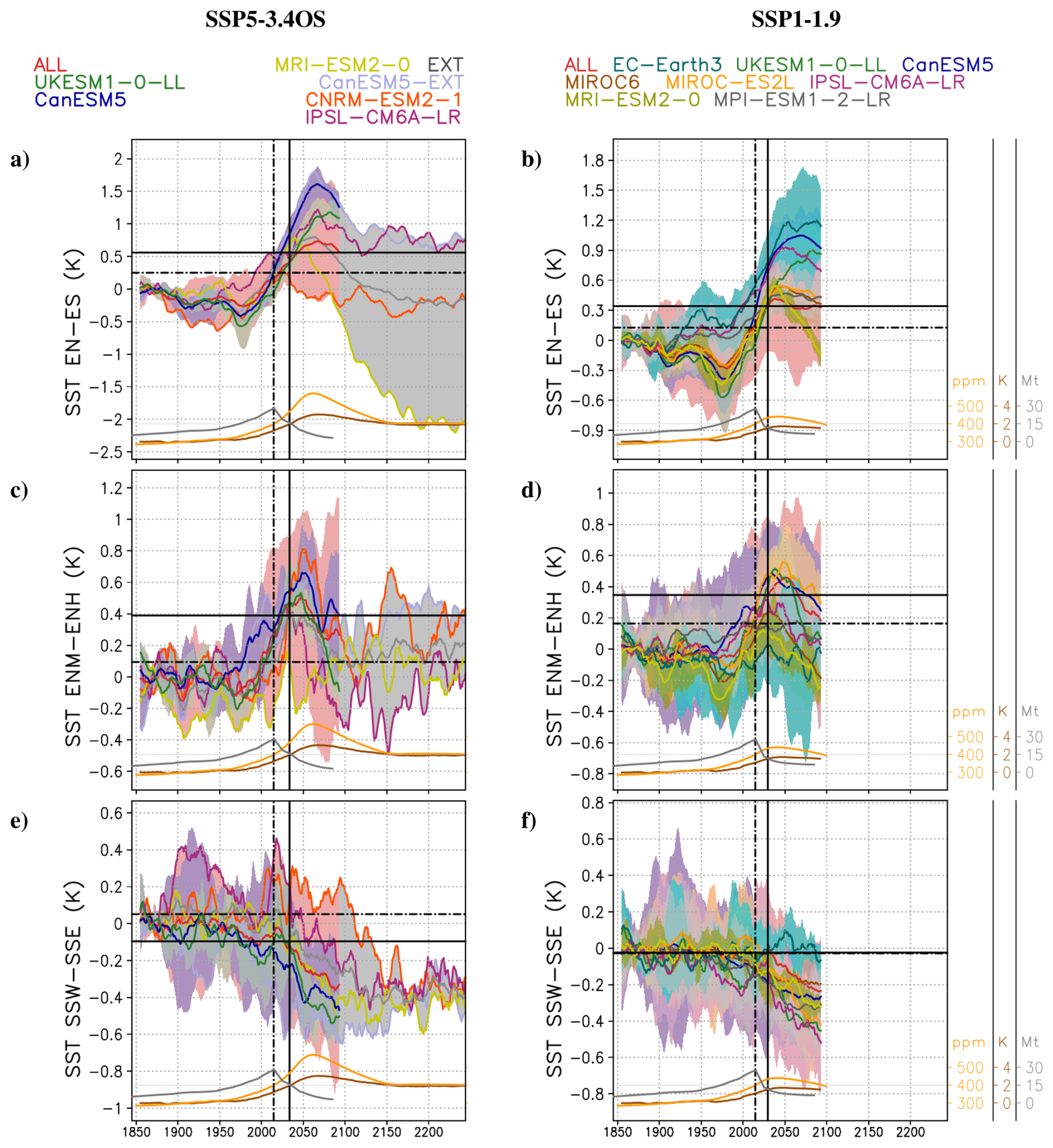
Figure 3 (a, b) Anomaly of Sea Surface Temperature (SST) difference between the extratropical ocean areas of the NH (EN) and the extratropical ocean areas of the SH (ES) with respect to 1861–1880, obtained from the CMIP6 simulations of experiments (a) SSP5-3.4OS and (b) SSP1-1.9, including the ALL and EXT ensembles, the ensemble average for each individual model and the individual extended simulations. Envelopes show the min–max values within each ensemble. Yellow, gray and brown curves in the lower part of each panel respectively show the CO₂ concentration from Meinshausen et al. (2020), the anthropogenic aerosol emissions from Feng et al. (2020), and the global surface air temperature obtained with the SSP1-1.9 ALL ensemble and the SSP5-3.4OS EXT ensemble. The vertical lines show the year before the overshoot with the same CO₂ concentration (dashed line) and global surface air temperature (solid line) as at the end of the run (2100 for the SSP1-1.9 ALL ensemble and 2300 for the SSP5-3.4OS EXT ensemble), while the horizontal lines represent the value of SST difference in the SSP1-1.9 ALL ensemble and in the SSP5-3.4OS EXT ensemble for those years. (c, d) Same as (a), (b), but for the mid-latitude extratropical ocean areas of the NH (ENM) and the high-latitude extratropical ocean areas of the NH (ENH). (e, f) Same as (a), (b), but for the south-western Southern Ocean (SSW) and the south-eastern Southern Ocean (SSE).

The comparison of different models (Fig. 3) for indices that represent the aforementioned asymmetries reveals that these asymmetries are not equally present in all models. For example, the simulations with MRI-ESM2-0 show a EN-ES asymmetry larger than 2 °C at the end of SSP5-3.4OS (year 2300; gold line of SST EN-ES in Fig. 3a) and close to 0.3 °C at the end of SSP1-1.9 (year 2100; gold line of SST ENM-ENH in Fig. 3b), while for other simulations like those with IPSL-CM6A-LR (purple line of SST EN-ES in Fig. 3a, b) this asymmetry is not clearly found. Something similar happens for the ENM-ENH asymmetry (Fig. 3c, d). Even if the averages of the SSP5-3.4OS EXT ensemble (gray line of SST ENM-ENH in Fig. 3c) and the SSP1-1.9 ALL ensemble (red line of SST ENM-ENH in Fig. 3d) show more negative values of ENM-ENH temperature after overshoot, this is only found for some simulations like those from MRI-ESM2-0 and IPSL-CM6A-LR (gold and purple lines of SST ENM-ENH in Fig. 3c, d), while some others like those from CNRM-ESM2-1 (dark orange line of SST ENM-ENH in Fig. 3c) or MIROC-ES2L (orange line of SST ENM-ENH in Fig. 3d) do not show a clear asymmetry. Fewer discrepancies exist for the SSW–SSE asymmetry (Fig. 3e, f), for which most model simulations show colder temperatures in the western sector after the overshoot, even if some particular simulations like those from EC-Earth3 show comparable temperatures in both regions (turquoise line of SST SSW–SSE in Fig. 3f).

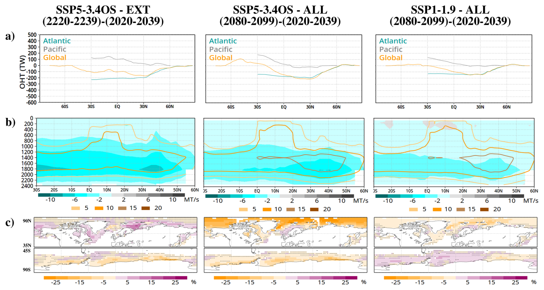
Figure 4 Difference between the ensemble mean, temporal average values of (a) Ocean Heat Transport (OHT; positive to the North), (b) Atlantic mass transport (positive to the South), and (c) sea ice concentration for (left) the periods 2220–2239 and 2020–2039 obtained with the SSP5-3.4OS EXT ensemble, (center) the periods 2080–2099 and 2020–2039 obtained with the SSP5-3.4OS ALL ensemble, and (right) the periods 2080–2099 and 2020–2039 obtained with the SSP1-1.9 ALL ensemble. Differences of OHT are shown per latitude, for the Atlantic basin, the Pacific basin, and the global zonal average. Differences of Atlantic mass transport are shown per latitude and level. Contours in (b) indicate climatological values of Atlantic mass transport obtained during the period 1861–1880. Stippling in (c) indicates locations where the differences are not significant (t-test with p<0.05).

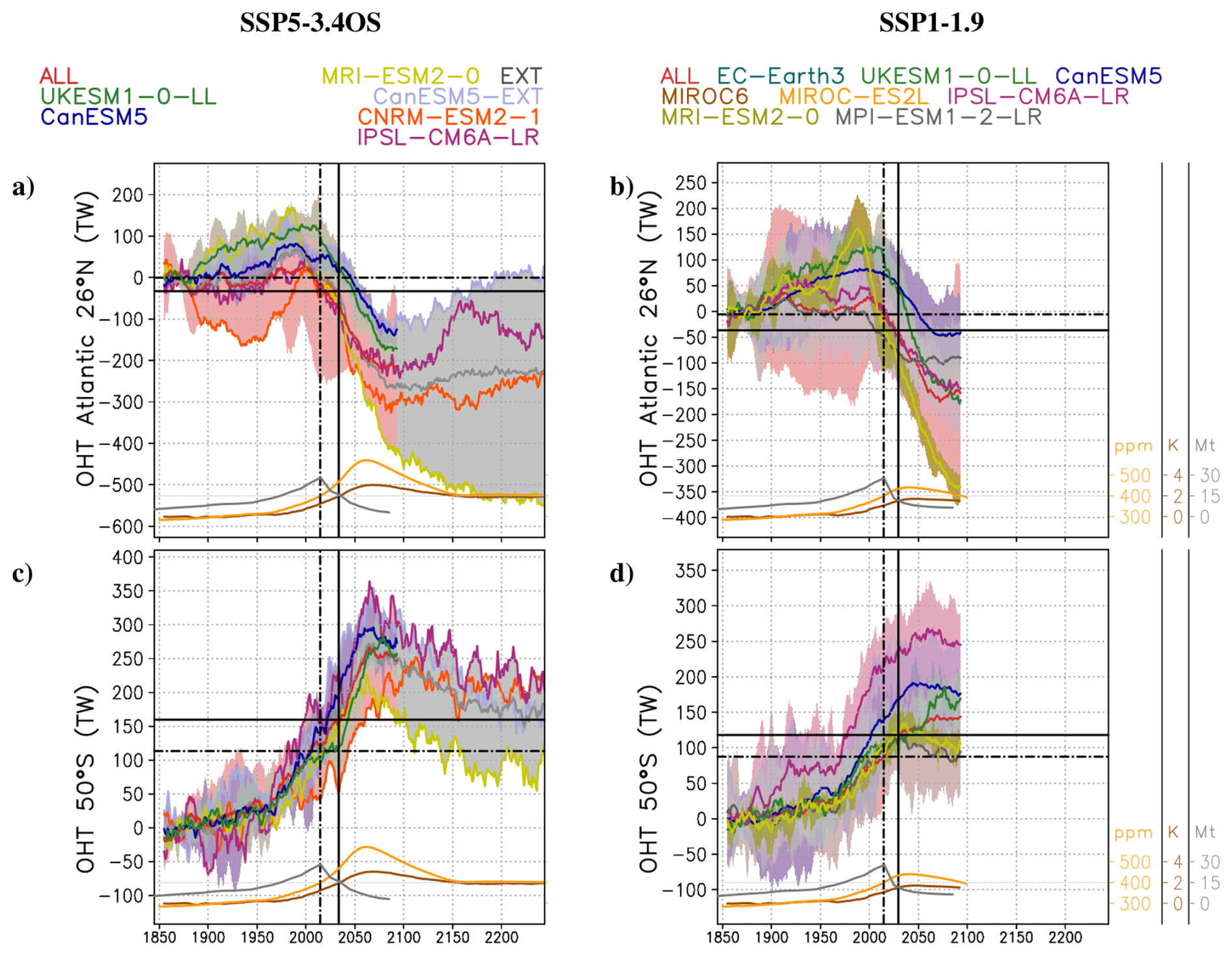
Figure 5 (a, b) Anomaly of Atlantic Ocean Heat Transport (OHT; positive to the North) at 26° N with respect to 1861–1880 obtained from the CMIP6 simulations of experiments (a) SSP5-3.4OS and (b) SSP1-1.9, including the ALL and EXT ensembles, the ensemble average for each individual model and the individual extended simulations. Envelopes show the min–max values within each ensemble. Yellow, gray and brown curves in the lower part of each panel respectively show the CO₂ concentration from Meinshausen et al. (2020), the anthropogenic aerosol emissions from Feng et al. (2020), and the global surface air temperature obtained with the SSP1-1.9 ALL ensemble and the SSP5-3.4OS EXT ensemble. The vertical lines show the year before the overshoot with the same CO₂ concentration (dashed line) and global surface air temperature (solid line) as at the end of the run (2100 for the SSP1-1.9 ALL ensemble and 2300 for the SSP5-3.4OS EXT ensemble), while the horizontal lines represent the value of Atlantic OHT at 26° N in the SSP1-1.9 ALL ensemble and in the SSP5-3.4OS EXT ensemble for those years. (c, d) Same as (a), (b), but for the global OHT at 50° S.

3.2 Meridional overturning circulation changes

The alteration of the meridional overturning circulation plays a major role on the regional hysteresis in case of overshoot (Li et al., 2024). Figure 4 shows the difference between post-overshoot (2220–2239 for SSP5-3.4OS EXT ensemble and 2080–2099 for SSP5-3.4OS and SSP1-1.9 ALL ensemble) and pre-overshoot (2020–2039) states for the global, Atlantic and Pacific OHT (Fig. 4a) and the Atlantic mass transport (Fig. 4b). In the multi-model average, the post-overshoot state is characterized by a lower northward OHT in the Atlantic basin (Fig. 4a), particularly between 30° S and 30° N, associated with a weakened meridional mass transport (Fig. 4b). Changes in the Atlantic Ocean mass transport are particularly strong where the overturning streamfunction attains its climatological maximum, that is between 1200 and 2000 m and between 30 and 40° N. In line with the analysis from Li et al. (2024) and Baker et al. (2025), the reduced heat transport in the Atlantic basin is partly compensated by increased northward OHT in the Pacific basin, between 30° S and the equator (Fig. 4a). In the Southern Ocean, higher values of northward OHT are found on average between 60 and 30° S for the SSP5-3.4OS ALL ensemble (Fig. 4a, center), but this is not the case for the SSP1-1.9 ALL ensemble (Fig. 4a, right) and the SSP5-3.4OS EXT ensemble (Fig. 4a, left). As for the case of temperatures, the temporal evolution of OHT for individual models (Fig. 5) highlights a strong inter-model dispersion. MRI-ESM2-0 shows a strong decrease in Atlantic OHT (gold line in Fig. 5a, b), while other models like CanESM5 and IPSL-CM6A-LR (blue and purple lines in Fig. 5a, b) show a more limited decrease. In the Southern Ocean, some models like CNRM-ESM2-1 (dark orange line in Fig. 5c) and IPSL-CM6A-LR (purple line in Fig. 5c, d) show a relevant strengthening of the northward OHT at the end of the run, while others like MRI-ESM2-0 (gold line in Fig. 5c, d) do not show relevant changes with respect to the pre-overshoot state.

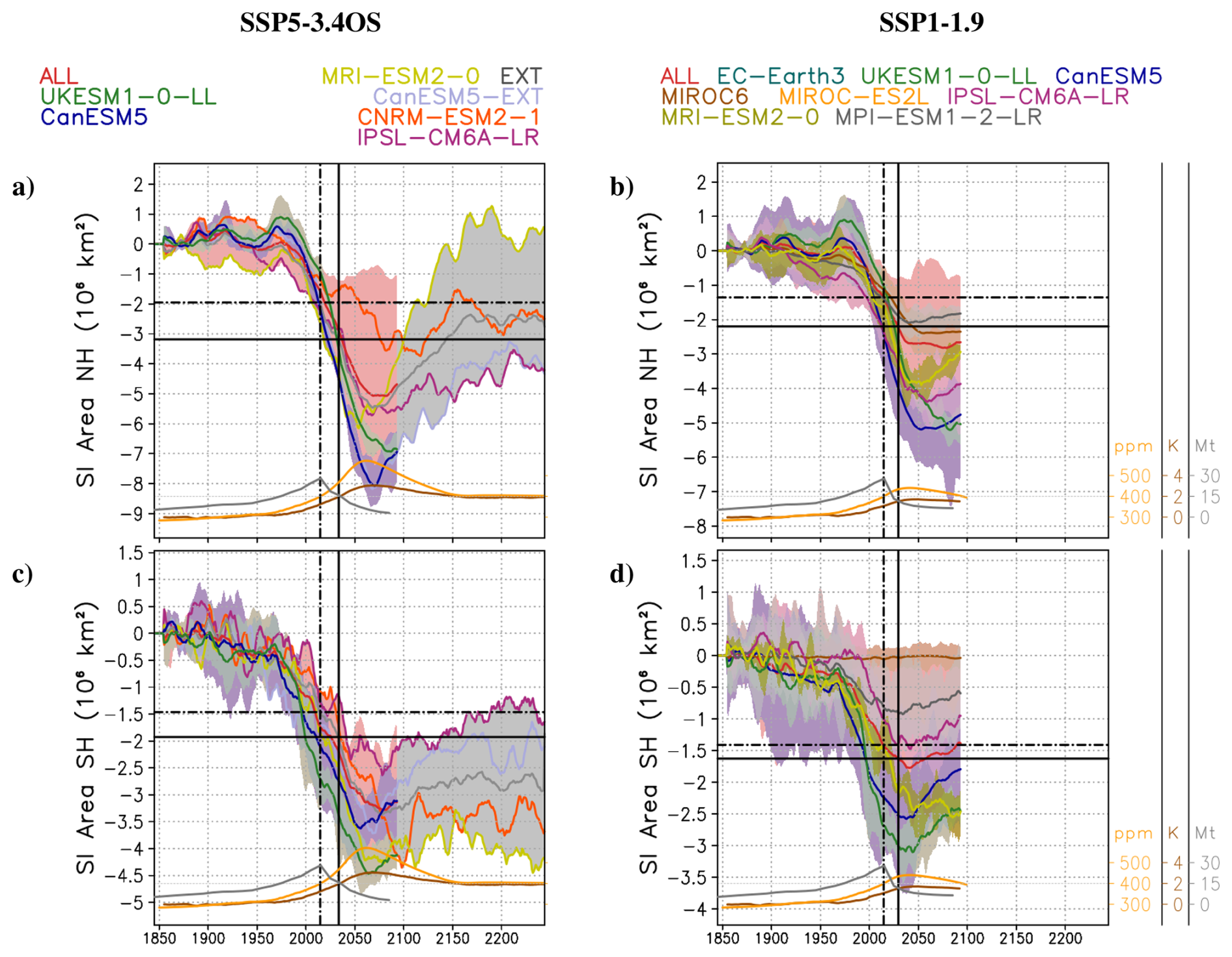
Figure 6 (a, b) Anomaly of Sea Ice (SI) area in the NH with respect to 1861–1880 obtained from the CMIP6 simulations of experiments (a) SSP5-3.4OS and (b) SSP1-1.9, including the ALL and EXT ensembles, the ensemble average for each individual model and the individual extended simulations. Envelopes show the min–max values within each ensemble. Yellow, gray and brown curves in the lower part of each panel respectively show the CO₂ concentration from Meinshausen et al. (2020), the anthropogenic aerosol emissions from Feng et al. (2020), and the global surface air temperature obtained with the SSP1-1.9 ALL ensemble and the SSP5-3.4OS EXT ensemble. The vertical lines show the year before the overshoot with the same CO₂ concentration (dashed line) and global surface air temperature (solid line) as at the end of the run (2100 for the SSP1-1.9 ALL ensemble and 2300 for the SSP5-3.4OS EXT ensemble), while the horizontal lines represent the value of SI area in the NH in the SSP1-1.9 ALL ensemble and in the SSP5-3.4OS EXT ensemble for those years. (c, d) Same as (a), (b), but for the SI area in the SH.

3.3 Sea ice changes

Hysteresis in the sea ice coverage is also identified as a mechanism potentially explaining irreversibility in temperature (Li et al., 2020). As shown in Fig. 4c, the post-overshoot state for the SSP5-3.4OS EXT ensemble average is characterized by higher sea ice concentrations in the NH and lower sea ice concentrations in the SH (Fig. 4c, left), a feature that can be linked to the reduced global northward heat transport. By contrast, for the SSP1-1.9 ALL ensemble lower concentrations are found in the eastern Southern Ocean and the NH and higher concentrations are found in the western Southern Ocean (Fig. 4c, right). These differences between SSP5-3.4OS and SSP1-1.9 can be explained by the different models represented in each ensemble, as individual models show highly heterogeneous sea ice responses. As shown in Fig. 6a, c, the average of the SSP5-3.4OS EXT ensemble (gray line) shows a larger sea ice area in the NH and a smaller sea ice area in the SH after overshoot, but this mean response is dominated by the simulations from MRI-ESM2-0 (gold line in Fig. 6a, c) and, to a lesser extent, CNRM-ESM2-1 (dark orange line in Fig. 6a, c). For the average of SSP1-1.9 ALL (red line in Fig. 6b, d), the behavior is the opposite, with smaller sea ice area in the NH and larger sea ice area in the SH after overshoot.

3.4 Contributions to temperature changes across different models

Considering the large discrepancies across the models in the simulation of temperature changes (Fig. 3), the OHT responses (Fig. 5), and the concomitant sea ice changes (Fig. 6), the contribution of each mechanism to large-scale temperature asymmetries must be analyzed on a per-model basis.

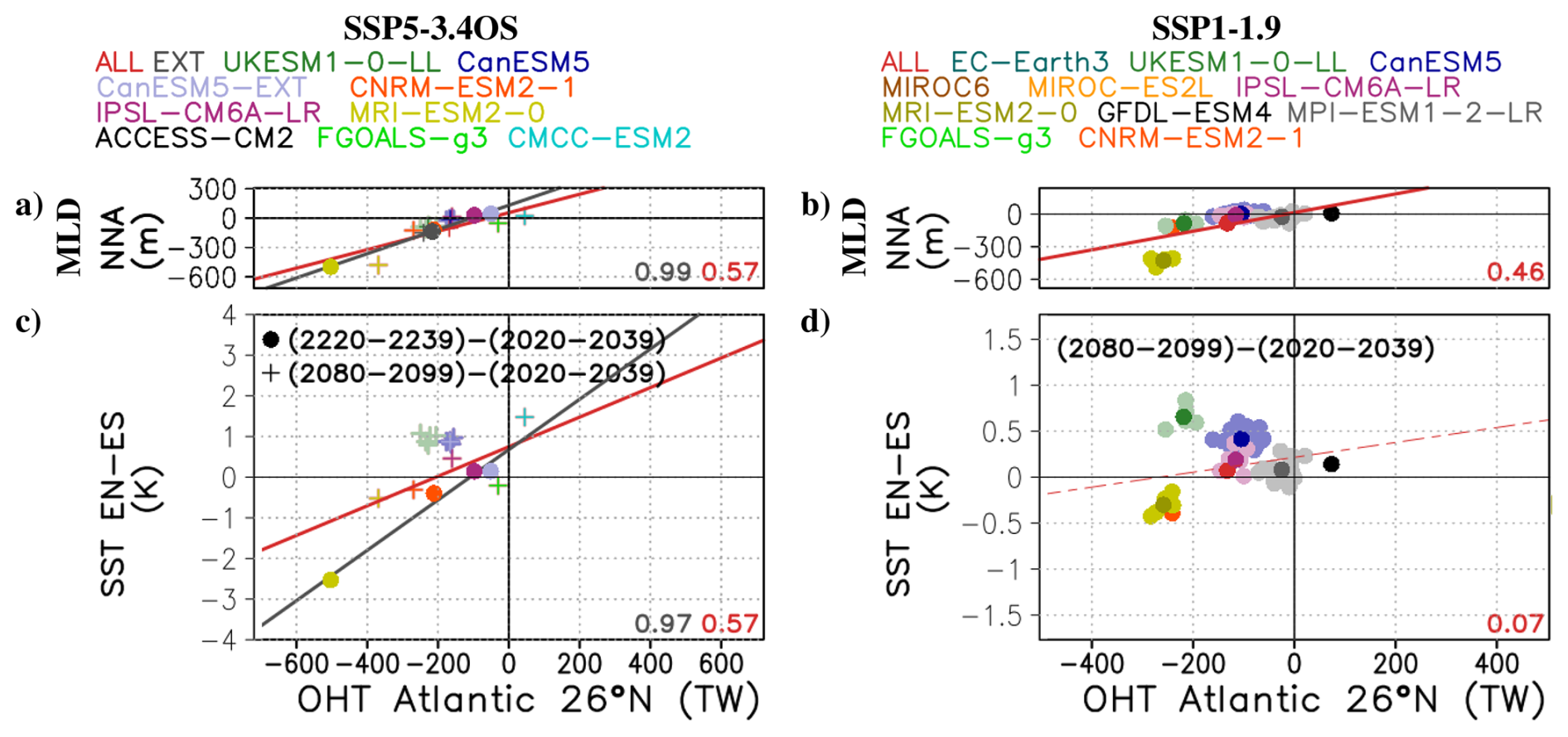
Figure 7 (a, b) March Mixed Layer Depth (MLD) in the northern North Atlantic (NNA) versus Atlantic Ocean Heat Transport (OHT) at 26° N for the periods 2220–2239 and 2080–2099 with respect to the reference period 2020–2039, obtained with each simulation of (a) SSP5-3.4OS and (b) SSP1-1.9, as well as with the ensemble average of all the models (ALL), the ensemble average of simulations extended up to 2300 (EXT), and the ensemble average of each model containing several simulations. Regression lines and coefficients of determination (R²) are included within the figures, both for EXT ensemble (gray) and ALL ensemble (red). Solid lines indicate that correlations are significant (t-test with p<0.05). (c, d) Sea Surface Temperature (SST) difference between extratropical ocean areas of the NH (EN) and extratropical ocean areas of the SH (ES) versus Atlantic OHT at 26° N for the periods 2220–2239 and 2080–2099 with respect to the reference period 2020–2039, obtained with each simulation of (c) SSP5-3.4OS and (d) SSP1-1.9, as well as with the ensemble average of all the models (ALL), the ensemble average of simulations extended up to 2300 (EXT), and the ensemble average of each model containing several simulations.

Figure 7c, d shows how the EN-ES temperature asymmetry – as characterized by the difference between the post-overshoot (2220–2239 and 2080–2099) and pre-overshoot (2020–2039) states – in individual simulations and their ensemble mean relate to changes in Atlantic OHT at 26° N. The models with the most negative differences in the northward Atlantic OHT, like MRI-ESM2-0 and CNRM-ESM2-1, are also those showing the coldest temperatures in EN with respect to ES. The R² coefficient between northward Atlantic OHT at 26°N and EN-ES asymmetry reaches 0.97 for SSP5-3.4OS EXT and 0.57 for SSP5-3.4OS ALL, both significant at a 95 % confidence level (Fig. 7c). Even if the high correlation for SSP5-3.4OS EXT may be explained by the limited number of simulations covering the period up to 2300 (only 4 simulations), these results show a clear relationship between Atlantic OHT and the hemispheric temperature asymmetries. For the case of SSP1-1.9, MRI-ESM2-0 and CNRM-ESM2-1 are also the models showing the strongest OHT reduction and EN-ES asymmetry, even if the ensemble averages do not support a linear relationship between both quantities (Fig. 7d). The relationship between Atlantic OHT at 26° N and the MLD in NNA (Fig. 7a, b) is almost linear, with significant correlations of 0.99 for SSP5-3.4OS EXT (Fig. 7a) and 0.46 for SSP1-1.9 ALL (Fig. 7b). Changes during the overshoot are significantly stronger for the models with the largest climatological values of MLD, with a R² coefficient between the post-overshoot MLD change and its reference climatology of 0.98 for SSP5-3.4OS EXT (Fig. 8a) and 0.52 for SSP1-1.9 ALL (Fig. 8b).

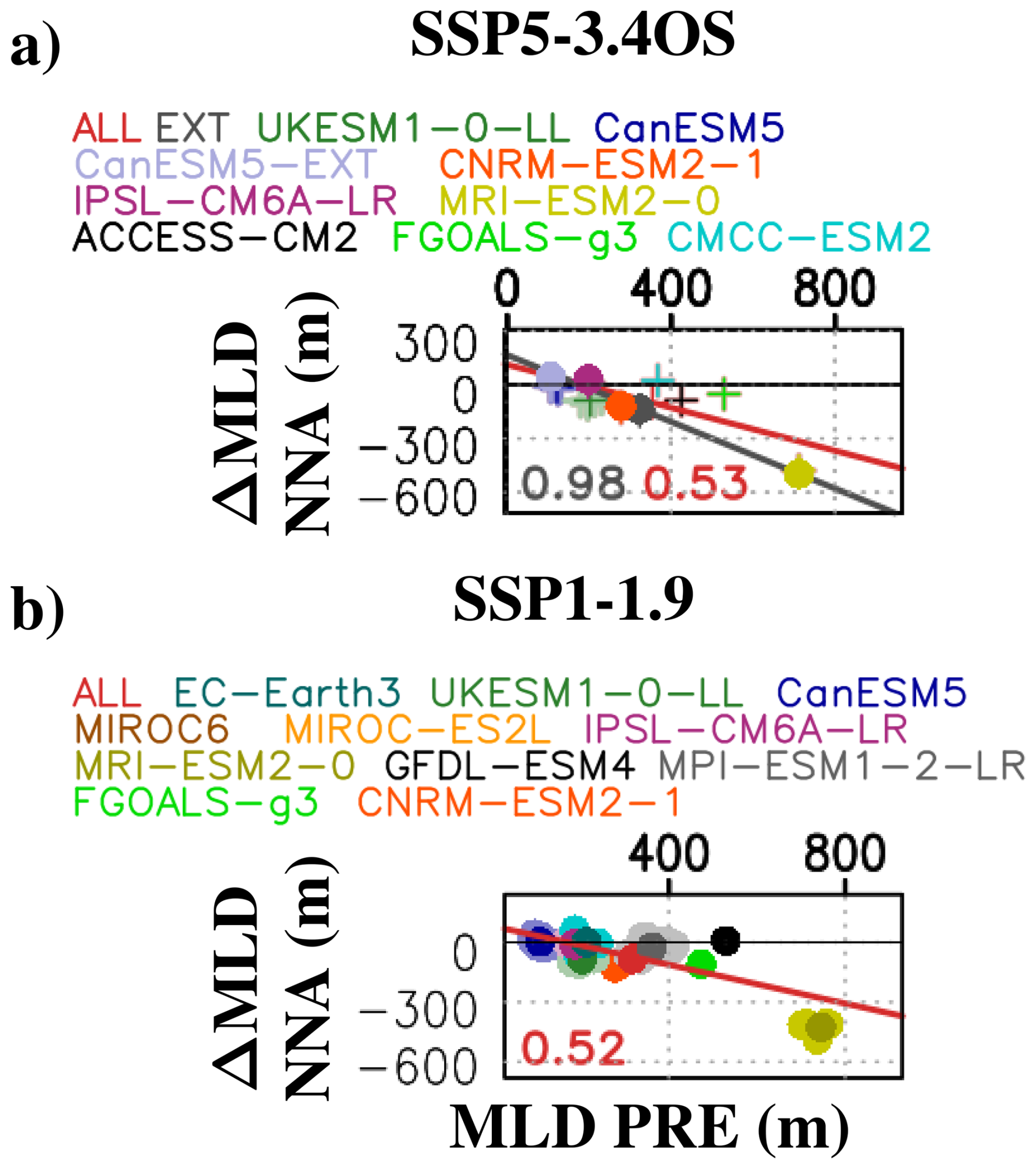
Figure 8 (a, b) March Mixed Layer Depth (MLD) in the northern North Atlantic (NNA) post-overshoot (2220–2239 and 2080–2099) to pre-overshoot (2020–2039) difference versus its climatology for the pre-industrial period (PRE; 1861–1880), obtained with each simulation of (a) SSP5-3.4OS and (b) SSP1-1.9, as well as with the ensemble average of all the models (ALL), the ensemble average of simulations extended up to 2300 (EXT), and the ensemble average of each model containing several simulations. Regression lines and coefficients of determination (R²) are included within the figures, both for EXT ensemble (gray) and ALL ensemble (red). Solid lines indicate that correlations are significant (t-test with p<0.05).

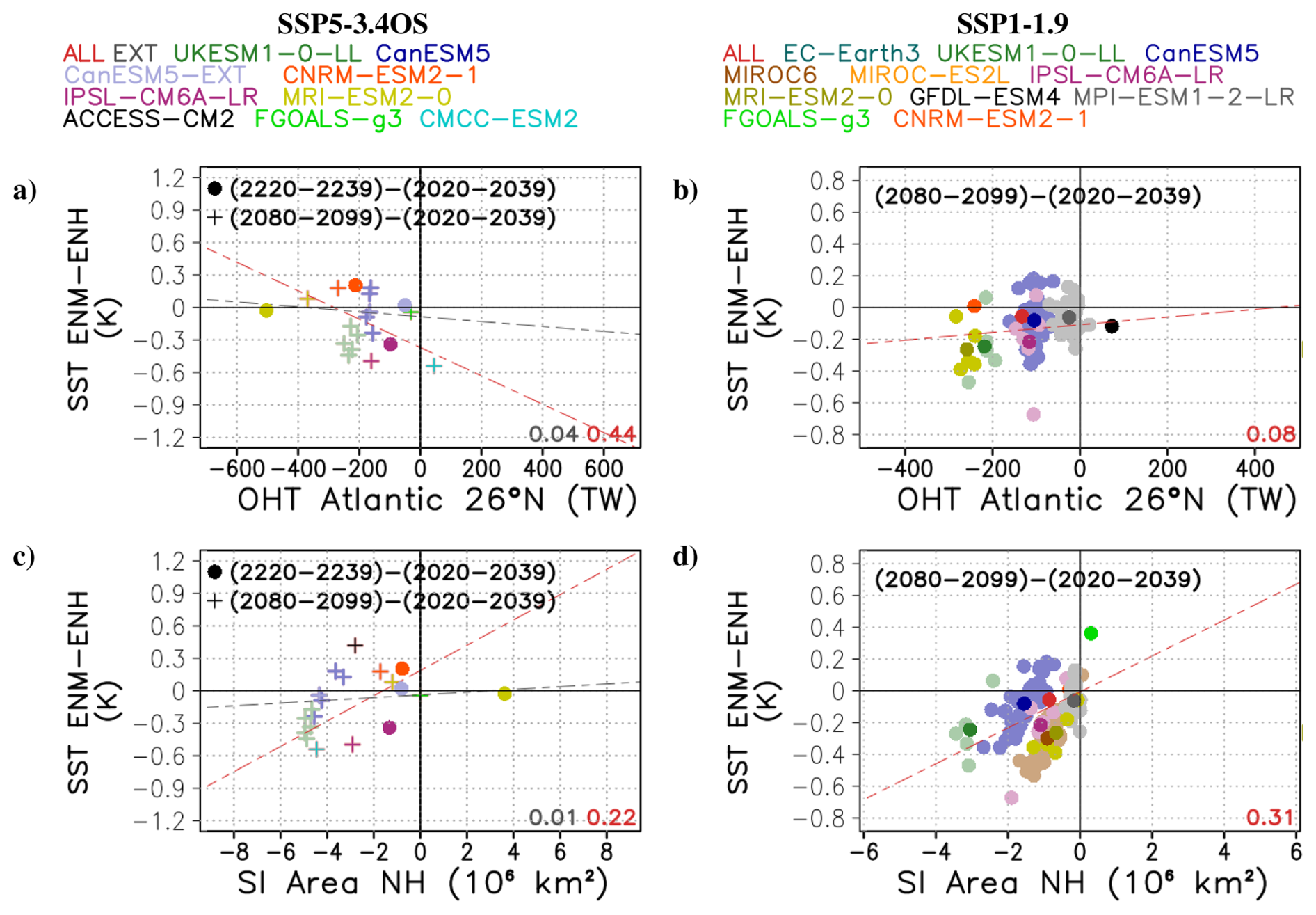
Figure 9 (a, b) Sea Surface Temperature (SST) difference between mid-latitude extratropical ocean areas of the NH (ENM) and high-latitude extratropical ocean areas of the NH (ENH) versus Atlantic Ocean Heat Transport (OHT) at 26° N for the periods 2220–2239 and 2080–2099 with respect to the reference period 2020–2039, obtained with each simulation of (a) SSP5-3.4OS and (b) SSP1-1.9, as well as with the ensemble average of all the models (ALL), the ensemble average of simulations extended up to 2300 (EXT), and the ensemble average of each model containing several simulations. Regression lines and coefficients of determination (R²) are included within the figures, both for EXT ensemble (gray) and ALL ensemble (red). Solid lines indicate that correlations are significant (t-test with p<0.05). (c, d) Same as in (a), (b), but for SST ENM-ENH differences versus Sea Ice (SI) area in the NH.

The ENM-ENH temperature asymmetry cannot be clearly linked to changes in the Atlantic OHT (Fig. 9a, b). A certain contribution of sea ice changes (Fig. 9c, d) is found for some of the models. Indeed, in models like UKESM1-0-LL, CMCC-ESM2, IPSL-CM6A-LR, CanESM5 and MIROC6 the individual simulations with a larger decline in the NH sea ice area after the overshoot, show the strongest ENM-ENH asymmetry. By contrast, simulations with weaker changes in the sea ice, like those from CNRM-ESM2-1, ACCESS-CM2, MPI-ESM1-2-LR, and FGOALS-g3, do not show relevant temperature asymmetries between the mid and high latitudes of the NH. Despite this consistent behavior, the R² coefficients when considering ensemble averages are small, with only 0.22 for SSP5-3.4OS ALL (Fig. 9c) and 0.31 for SSP1-1.9 ALL (Fig. 9d), evidencing important differences across the models. As shown in Fig. 9d, there are also important differences across the simulations from a given model, indicating that results can also be sensitive to internal variability. Interestingly, within some model ensembles, like those from CanESM5 and MIROC6, the simulations support a linear relationship between the changes in the sea ice area and the ENM-ENH asymmetries, indicating that in these models a relationship between sea ice area and SST is found associated with internal variability.

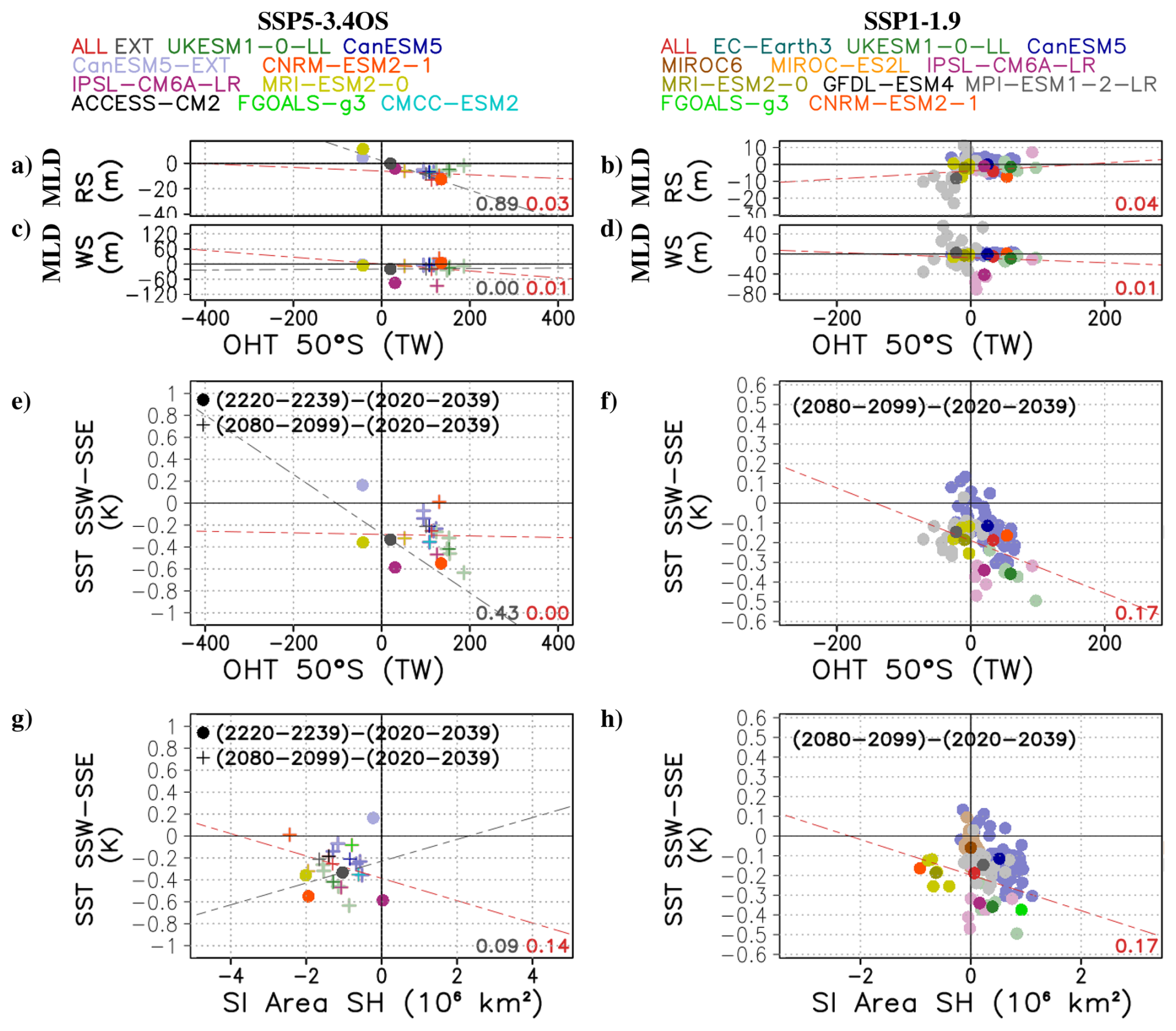
Figure 10 (a, b) September Mixed Layer Depth (MLD) in Ross Sea (RS) versus global OHT at 50° S for the periods 2220–2239 and 2080–2099 with respect to the reference period 2020–2039, obtained with each simulation of (a) SSP5-3.4OS and (b) SSP1-1.9, as well as with the ensemble average of all the models (ALL), the ensemble average of simulations extended up to 2300 (EXT), and the ensemble average of each model containing several simulations. (c, d) Same as in (a), (b), but for the September MLD in Weddell Sea (WS). (e, f) Sea Surface Temperature (SST) difference between south-western Southern Ocean (SSW) and south-eastern Southern Ocean (SSE) versus global Ocean Heat Transport (OHT) at 50° S for the periods 2220–2239 and 2080–2099 with respect to the reference period 2020–2039, obtained with each simulation of (e) SSP5-3.4OS and (f) SSP1-1.9, as well as with the ensemble average of all the models (ALL), the ensemble average of simulations extended up to 2300 (EXT), and the ensemble average of each model containing several simulations. Regression lines and coefficients of determination (R²) are included for all the panels, both for EXT ensemble (gray) and ALL ensemble (red). Solid lines indicate that correlations are significant (t-test with p<0.05). (g, h) Same as in (e), (f), but for SST SSW–SSE differences versus Sea Ice (SI) area in the SH.

The contribution of sea ice changes to the SSW–SSE asymmetry (Fig. 10g, h) seems marginal. Simulations with a larger increase in SH sea ice area, like those from CanESM5 and FGOALS-g3 in SSP1-1.9 (Fig. 10h), are not necessarily those with larger SSW–SSE asymmetries. A relevant contribution of the OHT at 50° S – which can be linked to the SMOC – to the SSW–SSE asymmetry is found (Fig. 10e, f), as the models with a larger OHT increase (e.g. UKESM1-0-LL, IPSL-CM6A-LR, and CNRM-ESM2-1) tend to simulate the largest temperature asymmetries. For the case of UKESM1-0-LL, this situation is also associated with a decrease in the MLD in the WS and RS regions (Fig. 10a–d), while for the IPSL-CM6A-LR the decrease is limited to the WS region (Fig. 10c, d), and for CNRM-ESM2-1 it is limited to the RS region (Fig. 10a, b), reflecting that the key areas of MLD in the Southern Ocean are highly model dependent. For the case of SSW–SSE asymmetry, the large spread among the models reduces the R² coefficient between OHT and temperature differences, to 0.43 for SSP5-3.4OS EXT (Fig. 10e) and to 0.17 for SSP1-1.9 ALL (Fig. 10f). Other factors like eddy compensation or wind stress changes may also have a relevant role in this area, contributing also to reduce the R² coefficient.

To better illustrate the different spatial patterns associated with these changes, comparisons between post-overshoot and pre-overshoot states are provided for individual models in Appendix B.

4 Discussion and conclusions

The analysis of CMIP6 overshoot scenarios (SSP5-3.4OS and SSP1-1.9) confirms that certain regions do not fully return to their pre-overshot state. This incomplete recovery is marked by persistent large-scale temperature asymmetries. Important temperature asymmetries are found between extratropical areas of the NH and SH, as well as between mid and high latitudes of the NH, and between eastern and western areas of the Southern Ocean. The relative role of these temperature asymmetries strongly depends on the model, with some models like MRI-ESM2-0 presenting strong asymmetries between NH and SH, some others like CNRM-ESM2-1 asymmetries between mid and high latitudes, and some models like IPSL-CM6A-LR and CanESM5 showing important asymmetries in the Southern Ocean.

These temperature asymmetries can be associated with several mechanisms introducing hysteresis in the climate system during the overshoot, including changes in ocean dynamics and meridional overturning circulation (Palter et al., 2018), both in the Atlantic and in the Southern Ocean (Li et al., 2024), as well as the melting of sea ice (Li et al., 2020). These processes are known to be inter-connected as revealed in the analysis of pre-industrial and global warming scenarios, with changes in OHT producing changes in sea ice, and altering then the MLD around Greenland (Meccia et al., 2022).

The post-overshoot situation is generally characterized by a weakened AMOC, with lower northward OHT in the Atlantic and a decrease in MLD around Greenland. An alteration of the SMOC is also present in some simulations, with a decrease in MLD and southward OHT in the Southern Ocean. In addition, the sea ice lost during the CO₂ increasing phase is not always fully recovered during the CO₂ decreasing phase. These changes can explain EN-ES, ENM-ENH, and SSW–SSE temperature asymmetries, being the simulations with the largest EN-ES asymmetries those with the largest reductions in the Atlantic OHT and MLD in NNA region, the simulations showing important ENM-ENH asymmetries those including a more limited recovery of NH sea ice after the overshoot, and the simulations with the largest SSW–SSE asymmetries those with the largest changes in the OHT in the Southern Ocean.

In line with Sgubin et al. (2017), the analyses performed in this work show that the contribution of each mechanism strongly depends on the model, with some models like MRI-ESM2-0 showing strong alterations of the AMOC, some models like CNRM-ESM2-1 highlighting persistent changes in the sea ice, and some others like IPSL-CM6A-LR and CanESM5 simulating a relevant impact of the SMOC. This model-dependent behavior highlights the current uncertainties for the simulation of the ocean circulation and sea ice responses, which are probably limited by the coarse resolutions considered for these experiments, unable to resolve potentially key contributions from mesoscale eddies and sea ice leads. The discrepancies between models can be associated with different climatological values for the MLD in the Subpolar North Atlantic region and in the Southern Ocean depending on the model. Models showing the largest climatological MLD also allow larger MLD decreases, producing a stronger AMOC slowdown, and then a larger hysteresis in the meridional overturning during the overshoot. Despite these preliminary results, a more detailed per-model analysis would be needed to fully understand the physical mechanisms explaining this relationship. Identifying such relationships between climatological characteristics and projected changes could enable potential emergent constraints (Hall et al., 2019), if a robust observational estimate of MLD could be obtained. The contribution of each mechanism may also depend on the individual simulation of a given model, suggesting a relevant role of internal variability. This is found for example in Fig. 9d, in which different ensemble members of CanESM5 and MIROC6 show a different relative contribution of NH sea ice changes to the ENM-ENH asymmetry.

This work provides a comprehensive analysis of CMIP6 overshoot scenarios, with the goal of identifying the main large-scale temperature patterns present in the post-overshoot climate and how ocean circulation and sea ice changes contribute to shaping these patterns. These analyses show a link between persistent changes in the OHT and sea ice after the overshoot and the emergence of temperature asymmetries in the post-overshoot climate, between NH and SH, between high and mid-latitudes of the NH and between eastern and western Southern Ocean. They also show substantial inter-model differences in the relative contributions of meridional overturning circulation and sea ice changes to these asymmetries. Such in-depth analysis of changes and associated processes across models is the basis to better understand projected changes and can ultimately help to reduce the uncertainty of expected changes. Additional efforts would be needed to better understand model differences with regard to ocean circulation and sea ice changes, while comparisons with observational data, in particular for the MLD and AMOC strength, could help to reduce model uncertainties.

Appendix A: Temperature asymmetries for Atlantic basin

Temperature asymmetries between NH and SH and between mid and high latitudes of the NH are analyzed based on the EN, ES, ENM and ENH regions defined in Fig. 1. These asymmetries are partly associated with changes in the AMOC, mainly focused on the Atlantic basin. To verify that the results are not sensitive to the selection of the regions, and in particular to the use of regions covering all basins, the same analyses are performed only for the Atlantic basin. In particular, Figs. A1 and A2 show the same results as for Figs. 2, 7 and 9 but considering the regions ENATL, ESATL and ENMATL. These regions are equivalent to EN, ES and ENM but considering only the Atlantic basin. For ENH, as this region mainly covers the Arctic Ocean, the per-basin separation is not meaningful.

Figure A2c, d shows a larger impact of the Atlantic OHT at 26° N in the ENMATL-ENH asymmetry than that obtained for the ENM-ENH asymmetry in Fig. 9a, b. The R² coefficient between OHT and temperature difference reaches 0.79 for SSP5-3.4OS EXT (Fig. A2c) and 0.75 for SSP1-1.9 ALL (Fig. A2d). Despite this minor difference, the results shown in Figs. A1 and A2 are generally in line with those from Figs. 2, 7 and 9, with ENATL-ESATL asymmetries behaving in a similar way as EN-ES asymmetries and ENMATL-ENH asymmetries behaving in a similar way as ENM-ENH asymmetries. This similarity confirms that even if the AMOC is mainly focused on the Atlantic basin, the changes in the OHT impact also the Southern Ocean and the Indo-Pacific basin (Li et al., 2024).

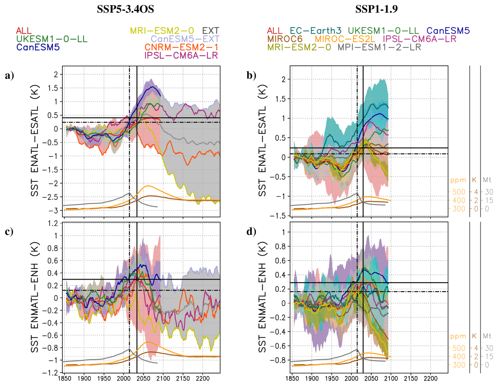
Figure A1 (a, b) Same as Fig. 2a, b, but for Atlantic extratropical areas of the NH (ENATL; 23–90° N; Atlantic basin) and Atlantic extratropical areas of the SH (ESATL; 90–23° S; Atlantic basin). (c, d) Same as Fig. 2a, b, but for Atlantic mid-latitude extratropical areas of the NH (ENMATL; 23–60° N; Atlantic basin) and high-latitude extratropical areas of the NH (ENH; 60–90° N).

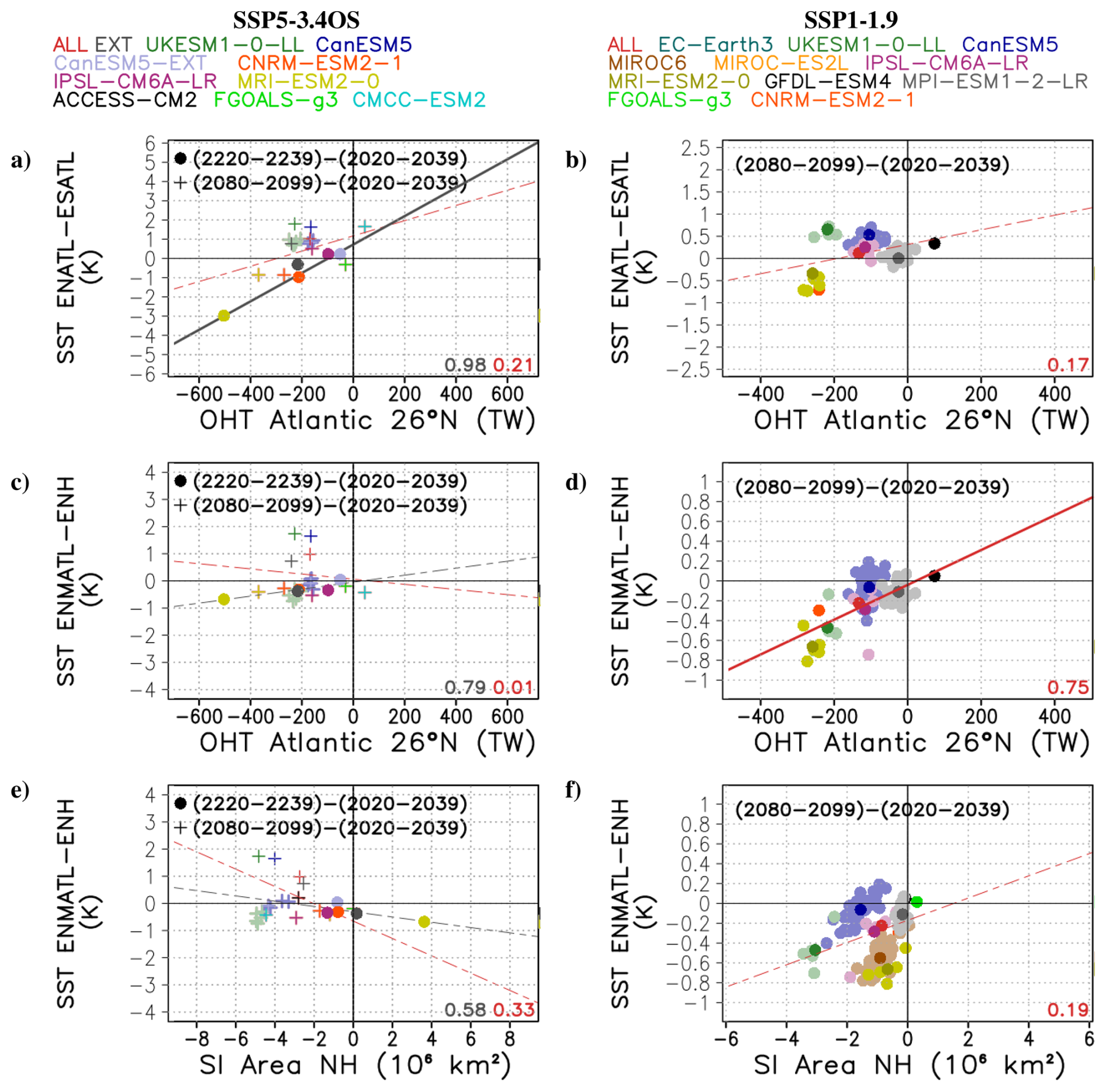
Figure A2 (a, b) Same as Fig. 7c, d, but for Atlantic extratropical areas of the NH (ENATL; 23–90° N; Atlantic basin) and Atlantic extratropical areas of the SH (ESATL; 90–23° S; Atlantic basin). (c, d) Same as Fig. 9a, b, but for Atlantic mid-latitude extratropical areas of the NH (ENMATL; 23–60° N; Atlantic basin) and high-latitude extratropical areas of the NH (ENH; 60–90° N). (e, f) Same as Fig. 9c, d, but for ENMATL and ENH.

Appendix B: Results for individual models

The post-overshoot state (2220–2239 for the SSP5-3.4OS EXT ensemble and 2080–2099 for the SSP5-3.4OS and SSP1-1.9 ALL ensembles) is compared with the pre-overshoot state (2020–2039) for all the models providing extended simulations of SSP5-3.4OS, namely, MRI-ESM2-0 (Fig. B1), CNRM-ESM2-1 (Fig. B2), IPSL-CM6A-LR (Fig. B3), and CanESM5 (Fig. B4). From these models, the simulations from MRI-ESM2-0 show very clear EN-ES asymmetries (Fig. B1a), while the simulations from CNRM-ESM2-1 show more prominent ENM-ENH asymmetries (Fig. B2a), and the simulations from IPSL-CM6A-LR show larger SSW–SSE asymmetries (Fig. B3a).

The simulations from MRI-ESM2-0 (Fig. B1) are characterized by strong changes of the AMOC, reflected as strong changes in the Atlantic OHT between 30° S and 30° N (Fig. B1b), the Atlantic mass transport (Fig. B1c) and the MLD around Greenland (Fig. B5a). These strong changes, which can be linked to the particularly large climatological values of MLD in NNA simulated by this model, generate a strong temperature asymmetry between extratropical areas of the NH and SH (Fig. B1a). In the NH, an asymmetry is also found between mid-latitude areas (with lower temperatures after the overshoot) and high-latitude areas (with higher temperatures instead) even if this ENM-ENH asymmetry is less prominent than the EN-ES asymmetry. The strong temperature asymmetry between NH and SH impacts also the sea ice distribution (Fig. B1d), which is generally increased in the NH and decreased in the SH. Only some areas of the NH around Greenland and Barents Sea show a relative decrease for the case of SSP1-1.9 and SSP5-3.4OS up to 2100.

The simulations from CNRM-ESM2-1 (Fig. B2) are characterized by strong sea ice changes (Fig. B2d). Both for the NH and SH, the sea ice lost during the CO₂ increasing phase is not fully recovered during the CO₂ decreasing phase (Fig. B2d), generating higher ocean surface temperatures in the polar areas after overshoot (Fig. B2a). Even if smaller in magnitude than those of MRI-ESM2-0, relevant changes are also found in the AMOC and its associated variables, with lower northward Atlantic OHT after overshoot (Fig. B2b), a decrease in the Atlantic mass transport (Fig. B2c) and a lower MLD around Greenland, extending up to the North Sea (Fig. B5b). The smaller changes with respect to MRI-ESM2-0 can be linked to smaller climatological values of MLD in NNA. Changes of MLD are limited to those areas with the largest climatological values, including a decrease in MLD in some areas of Labrador sea and the eastern subpolar North Atlantic that could explain the AMOC weakening, and an increase north of Iceland, potentially associated with a lack of sea ice recovery after overshoot. In the Southern Ocean, the OHT at 50° S is slightly increased in the post-overshoot situation (Fig. B2b), and a small increase in MLD is found in the WS area, where sea ice experiences a post-overshot decline (Fig. B2c).

The simulations from IPSL-CM6A-LR (Fig. B3) are characterized by important changes in the Southern Ocean, with an increase in the OHT at 50° S (Fig. B3b) and an important decrease in the MLD in the WS, the Southern Ocean region with the largest climatological values (Fig. B5c). These regional changes in the Southern Ocean may explain higher temperatures in SSE and lower temperatures in SSW after overshoot (Fig. B3a). The SSW–SSE temperature asymmetry can be linked to an asymmetry in the sea ice concentration, which experiences a decrease for SSE and an increase for SSW after overshoot (Fig. B3d). In the NH, there is a widespread decrease in sea ice concentrations (Fig. B3d), in line with the results from CNRM-ESM2-1 (Fig. B2d). The simulations from IPSL-CM6A-LR present very low climatological values of MLD in NNA, that experience a moderate strengthening after the overshot. These MLD changes cannot thus explain the weakening observed for the AMOC after the overshoot (Fig. B3c), accompanied by a decrease in the northward Atlantic OHT (Fig. B3b), changes that are, however, smaller in magnitude than those simulated by MRI-ESM2-0 and CNRM-ESM2-1.

The simulations from CanESM5 (Fig. B4) also show relevant changes in the Southern Ocean, with an increase in the OHT at 50° S (Fig. B4b) similar to that of IPSL-CM6A-LR (Fig. B3b) but without a clear strengthening of the MLD in the WS (Fig. B5d). In the NH, an ENM-ENH asymmetry is also found (Fig. B4b), potentially associated with a lack of recovery of NH sea ice after overshoot, as for the case of CNRM-ESM2-1 (Fig. B2d). As for the case of IPSL-CM6A-LR, the simulations of CanESM5 present low climatological values of MLD in NNA that are moderately strengthened after the overshoot, thus again decoupled from the observed weakening of the AMOC (Fig. B4c) and the northward Atlantic OHT (Fig. B4b), both smaller than for MRI-ESM2-0 and CNRM-ESM2-1. As for the case of IPSL-CM6A-LR, the retreat of sea ice coverage after overshoot increases the MLD in some areas of the eastern North Atlantic.

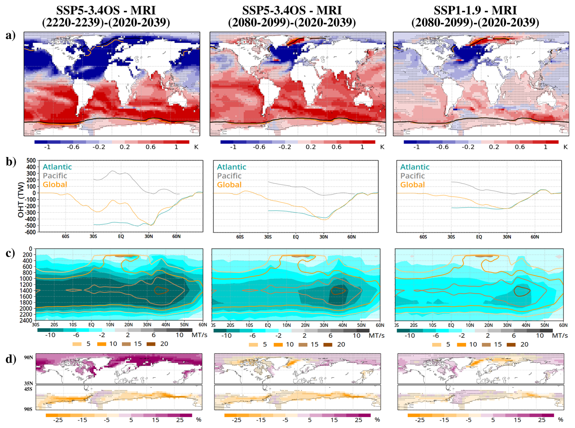
Figure B1 (a–d) Difference between the ensemble mean, temporal average values of (a) Sea Surface Temperature (SST), (b) Ocean Heat Transport (OHT; positive to the North), (c) Atlantic mass transport (positive to the South), and (d) sea ice concentration for (left) the periods 2220–2239 and 2020–2039 obtained with the MRI-ESM2-0 simulation of SSP5-3.4OS, (center) the periods 2080–2099 and 2020–2039 obtained with the MRI-ESM2-0 simulation of SSP5-3.4OS, and (right) the periods 2080–2099 and 2020–2039, obtained with the MRI-ESM2-0 ensemble of SSP1-1.9. Contours of 15 % of sea ice concentration are included in the maps of SST, both for the periods 2220–2239 and 2080–2099 (yellow) and for the reference period 2020–2039 (black). Differences of OHT are shown per latitude, for the Atlantic basin, the Pacific basin, and the global zonal average. Differences of Atlantic mass transport are shown per latitude and level. Contours indicate climatological values of Atlantic mass transport obtained with the period 1861–1880. Stippling indicates locations where the differences are not significant (t-test with p<0.05).

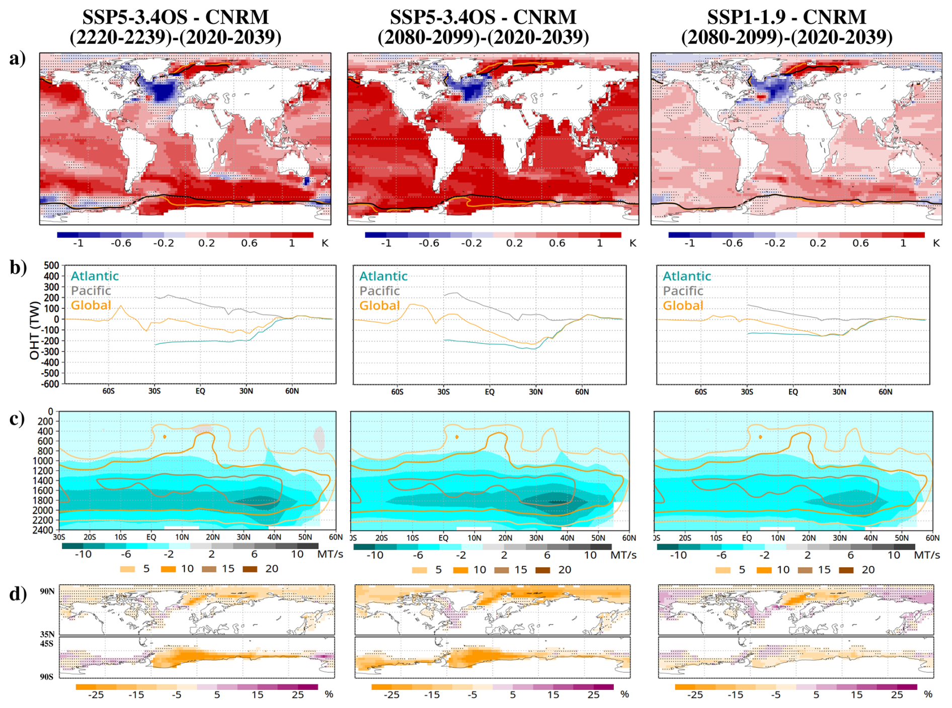
Figure B2 Same as Fig. B1, but for the CNRM-ESM2-1 model.

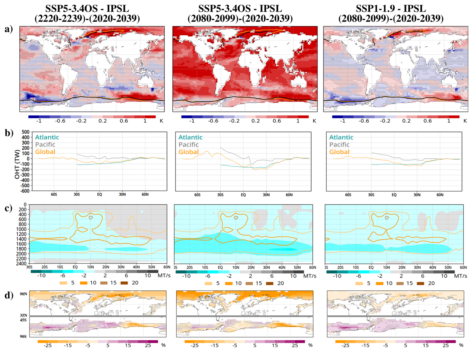
Figure B3 Same as Fig. B1, but for the IPSL-CM6A-LR model.

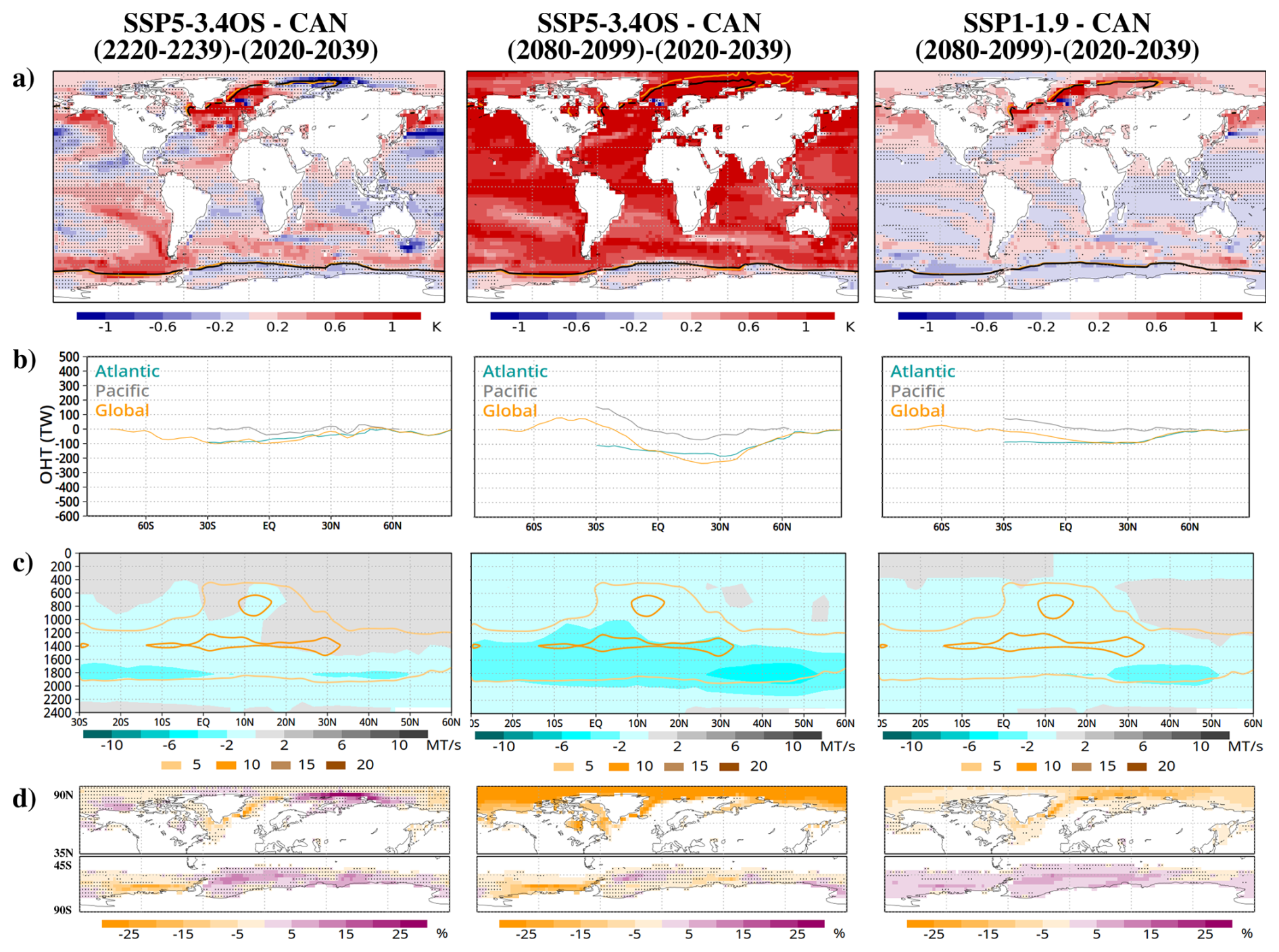
Figure B4 Same as Fig. B1, but for the CanESM5 model.

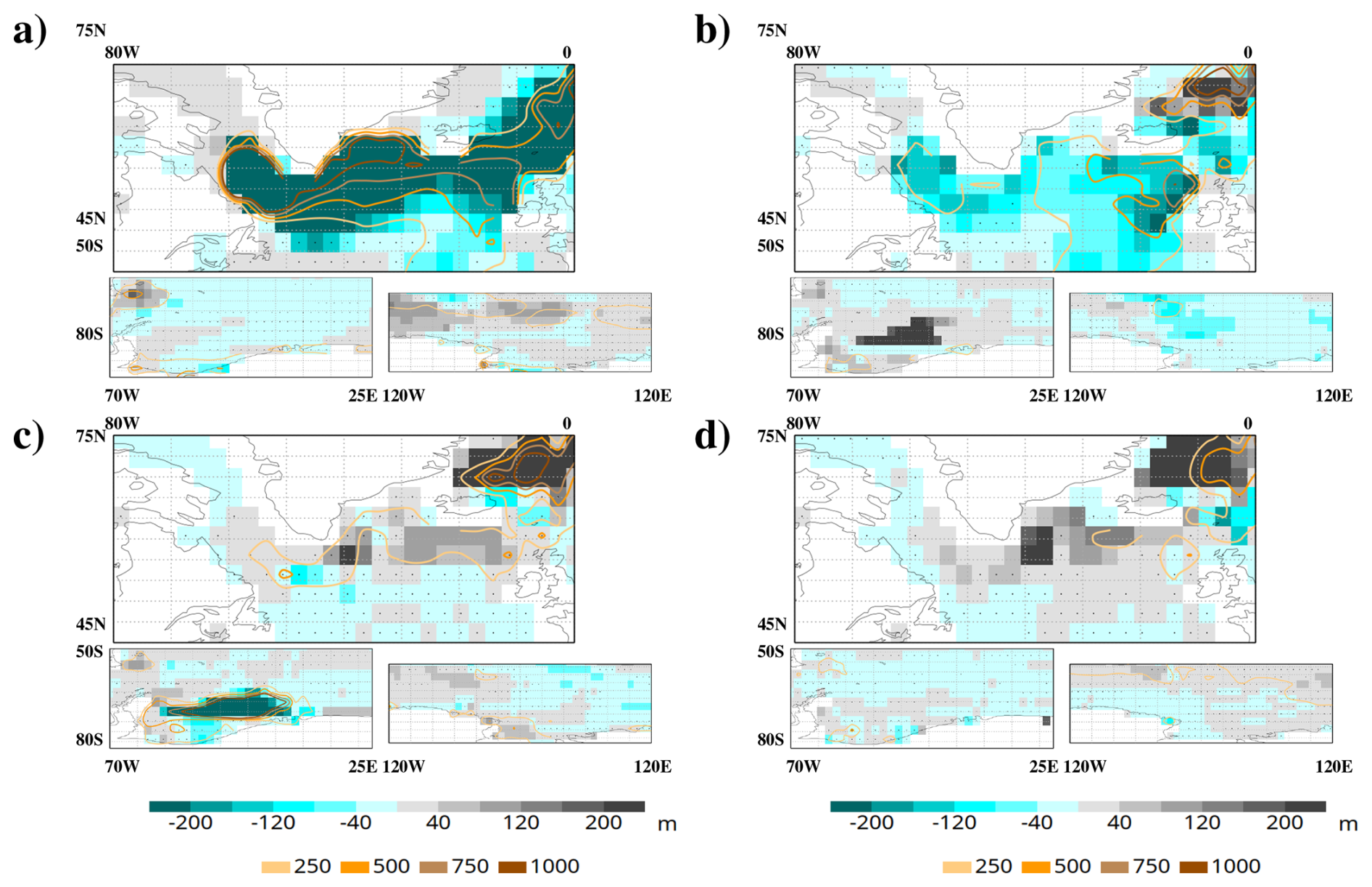
Figure B5 Difference between the ensemble mean, temporal average values of March Mixed Layer Depth (MLD) in the northern North Atlantic (NNA) and September MLD in Weddell Sea (WS) and Ross Sea (RS) for the periods 2220–2239 and 2020–2039 obtained with the extended SSP5-3.4OS simulations of (a) MRI-ESM2-0, (b) CNRM-ESM2-1, (c) IPSL-CM6A-LR, and (d) CanESM5. Contours indicate climatological values of MLD obtained with the period 1861–1880. Stippling indicates locations where the differences are not significant (t-test with p<0.05).