Multiscale phytoplankton dynamics in a coastal system of the eastern English Channel: the Boulogne-sur-Mer coastal area

To study changes in phytoplankton community composition on different timescales, an automated flow cytometer (CytoSub, CytoBuoy b.v.) was deployed at the MAREL Carnot automated monitoring station in Boulogne-sur-Mer (eastern English Channel, France) during spring (2021 and 2022) and summer (2022), following an Eulerian approach. Phytoplankton dynamics were recorded every 2 h, distinguishing 11 phytoplankton functional groups (PFGs) based on optical and fluorescence properties. This enabled detailed characterization of PFG successions, including MicroRED (mostly diatoms) and NanoRED (mostly haptophytes of the species Phaeocystis globosa) transitions in spring, as well as a summer dominance by PicoORG (picocyanobacteria, mostly of the genus Synechococcus) and PicoRED. Four rare events, including a salinity drop (April 2021), strong winds (May 2021 and April 2022), and a marine heat wave (July 2022), caused rapid shifts in phytoplankton community assemblage. Empirical mode decomposition (EMD) and Lomb–Scargle periodogram (LSP) analyses revealed that 85±10 % of variability in total phytoplankton abundance, red fluorescence (a proxy of chlorophyll a), and Shannon diversity occurred on relatively short timescales (9 h to 11 d) for time series of several months, highlighting the value of high-frequency monitoring in capturing ecological dynamics under macrotidal conditions in the eastern English Channel.

1 Introduction

Phytoplankton, comprising unicellular autotrophic organisms suspended in the water column, are key primary producers in marine ecosystems, driving carbon fixation and supporting heterotrophic organisms (Falkowski et al., 2003; Pal and Choudhury, 2014). They play a central role in marine food webs, including the microbial food web (Legendre and Rassoulzadegan, 1995), biogeochemical cycles, and the carbon biological pump. Despite constituting less than 0.1 % of the global biomass, phytoplankton contribute approximately half of the world's annual net primary production (Falkowski et al., 1998; Field et al., 1998; Bar-On et al., 2018; Bar-On and Milo, 2019).

Coastal zones, defined as transitional areas between marine and terrestrial environments which cover 12 % of Earth's surface and accommodate between 23 % and 50 % of the global population (Crossland et al., 2005), are highly dynamic environments with significant ecological and socioeconomic importance. These regions support 90 % of global fishing activity and exhibit high primary production driven by nutrient enrichment (Crossland et al., 2005; Cloern et al., 2014). Monitoring phytoplankton in these zones provides valuable insights into ecosystem health, helps us to better understand local ecosystems, and offers indirect socioeconomic benefits (Holland et al., 2023; Louchart et al., 2023). Coastal waters are characterized by high spatiotemporal variability influenced by natural and anthropogenic factors, making them ideal for high-frequency studies, which can capture rapid phenomena occurring within hours (Dubelaar et al., 2004; Kbaier Ben Ismail et al., 2016), and elucidating the strong spatiotemporal variability linked to mesoscale and submesoscale processes (Rantajärvi et al., 1998; Bonato et al., 2015). These studies are especially valuable for understanding processes like harmful algal blooms (HABs; Serre-Fredj et al., 2021) and multiscale phytoplankton dynamics in connection with multiscale changes in coastal water states (Hynes et al., 2024).

Phytoplankton dynamics respond rapidly to environmental changes driven by abiotic factors (e.g., light, turbulence, nutrients, temperature, and salinity) and biotic factors (e.g., competition, predation, and parasitism; Smith and Lancelot, 2004; Menge and Weitz, 2009; Wyatt, 2014; Chiswell et al., 2015). Understanding these responses requires monitoring approaches that capture temporal variability. Eulerian and Lagrangian frameworks are often employed, but interpreting time series data can be challenging due to the interplay between spatial and temporal changes.

In this study, we deployed an automated submersible “pulse-shape-recording” flow cytometer, associated with physicochemical parameters, at a coastal monitoring station in the eastern English Channel (EEC). This instrument performs optical single-cell measurements every 2 h, capturing phytoplankton dynamics from picophytoplankton (1 µm) to microphytoplankton (800 µm width; Olson et al., 2003; Dubelaar et al., 2004; Pomati et al., 2013; Fontana and Pomati, 2014; Pereira et al., 2017; Fragoso et al., 2019; Louchart et al., 2020). High-frequency cytometry measurements previously revealed insights into growth rates, physiological responses to rare events, and community variability (Sosik et al., 2010; Dugenne et al., 2014; Thyssen et al., 2014). By deploying the automated flow cytometry in an Eulerian framework in a highly dynamic system subject to anthropogenic pressure, we aimed to track phytoplankton variability across multiple timescales, capturing both periodic (e.g., tidal cycles) and non-periodic (e.g., rare events) changes in functional groups and community assemblage. This approach allowed us to explore phytoplankton dynamics over hours to months, enhancing our understanding of EEC coastal ecosystem variability.

2 Materials and methods

2.1 MAREL Carnot station

The MAREL Carnot station is an automated measurement platform that is part of the National Observation Service and integrated into the COAST-HF network (https://coast-hf.fr, last access: 12 December 2024). It is integrated into the French National Structure for Littoral and Coastal Observation (IR ILICO) infrastructure (https://www.ir-ilico.fr, last access: 12 December 2024) dedicated to high-frequency monitoring of French coastal environments (Halawi Ghosn et al., 2023; MAREL Carnot, 2024). The station is situated at the end of the 2 km long Carnot dike (50°44^′25.8^′′ N, 1°34^′3.72^′′ E) near the lighthouse at the entrance to Boulogne-sur-Mer harbor (Pas-de-Calais, France) at the mouth of the Liane estuary (Fig. 1). The depth of this area ranges between 5 and 16 m, with a mean depth of approximately 10 m (Halawi Ghosn et al., 2023). This coastal area is subject to significant anthropogenic pressures, including those from harbor activities but also agricultural runoff entering the river (Lheureux et al., 2023). This station continuously monitors subsurface (1.5 m depth) physicochemical parameters at 20 min intervals, including sea surface temperature (SST), salinity, turbidity, dissolved oxygen, wind direction and speed, and fluorescence, with a multiparameter sensor (NKE MP6) and a static weather station (AirMAR 200WX). A comprehensive description of these parameters is provided in Halawi Ghosn et al. (2023). As a fixed monitoring platform, it enables Eulerian observation of the marine environment by continuously recording temporal variations at a single location.

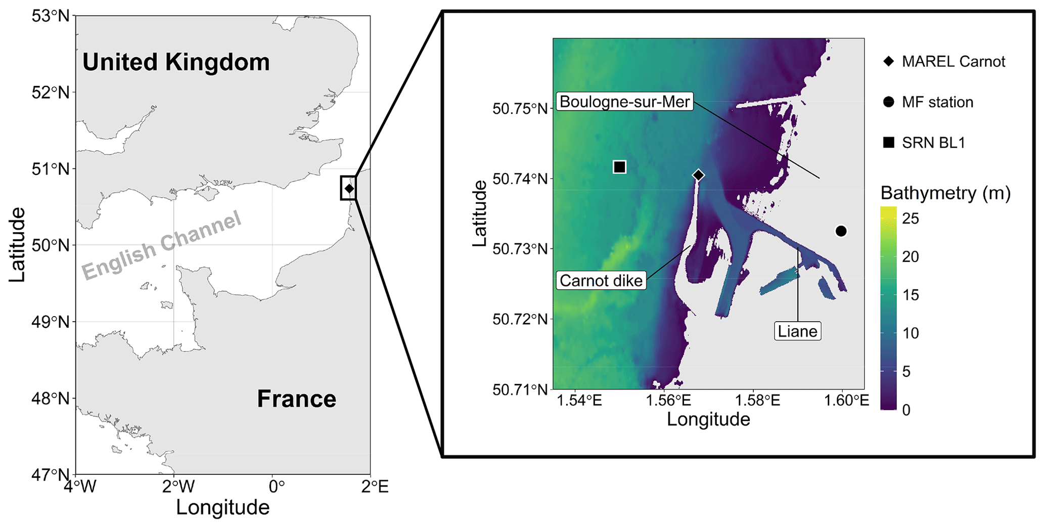
Figure 1 Map of the study area showing the location of the MAREL buoy on the Carnot dike in Boulogne-sur-Mer. The bathymetry data, with an approximate resolution of 10 m, were developed as part of the TANDEM project (SHOM, 2015). Only regions with bathymetric depths of more than 0 m are displayed. The MAREL Carnot, Météo-France (MF; 2.43 km from MAREL Carnot), and SRN Boulogne 1 (BL1; 1.25 km from MAREL Carnot) stations are indicated.

Wind data for 2021 were sourced from Météo-France (50°43^′57^′′ N, 1°35^′59^′′ E) due to a lack of available data from the MAREL Carnot station during that period. Additionally, water height data for 2021 and 2022 were obtained from the Réseaux marégraphiques français (REFMAR) data of the Service Hydrographique et Océanographique de la Marine (SHOM, France). Furthermore, low-frequency nutrient data (ammonium, nitrite, nitrate, phosphate, and silicate) from the Suivi Régional des Nutriments (SRN) program were utilized at the Boulogne 1 SRN station (50°43^′90^′′ N, 1°33^′00^′′ E) off the Boulogne-sur-Mer coastal area (the nearest low-frequency monitoring station with fortnightly 0.5 to 1 m depth sampling), as these parameters were not monitored by the MAREL Carnot station (Lefebvre et al., 2024). The 2021 and 2022 data are presented in Fig. 2.

Figure 2 SRN nutrient data (Lefebvre et al., 2024) at the Boulogne 1 station for 2021 and 2022. The two study periods are highlighted by the dashed lines (orange for 2021 and red for 2022).

The complex currents and the presence of multiple estuaries in the EEC (from the Somme estuary in Picardy, including the Liane estuary in Boulogne-sur-Mer, to the Slack estuary near the Strait of Dover, in addition to remote influence by the Seine estuary) contribute to the formation of the “coastal flow” (Brylinski et al., 1991). This region of freshwater influence (ROFI) affects physicochemical parameters, such as nutrients and salinity, which are influenced by freshwater discharge from local or remote estuaries and land-based streams entering the sea. Along a coastal strip spanning 3 to 5 nautical miles, brackish waters are observed, separated from the open sea by an interface similar to a desalination and tidal front (Brylinski et al., 1991). These conditions significantly shape phytoplankton dynamics, particularly during recurrent seasonal events such as the spring bloom, which is dominated in this region by an alternance of diatoms and haptophytes (Phaeocystis globosa; Breton et al., 2000; Lefebvre et al., 2011; Breton et al., 2022). The coastal waters off Boulogne-sur-Mer are characterized by a macrotidal regime (tidal range > 4 m) and occasionally border on mega-tidal conditions (tidal range > 8 m; Levoy et al., 2000). The tides are semidiurnal, completing a full cycle approximately every 12.4 h (Lazure and Desmare, 2012). During ebb tide, the current in the EEC flows southwestward, while flood tide results in a northeastward flow, causing a reversal in currents during tidal shifts. However, wind dynamics can significantly alter this circulation pattern, adding to the complexity of the hydrodynamics of the EEC at various spatiotemporal scales (Lazure and Desmare, 2012; Bertin et al., 2024). The current patterns within the harbor are also influenced by factors such as freshwater inflows and tidal phases, with an eddy typically forming during rising tide (Jouanneau et al., 2013; Sentchev and Yaremchuk, 2016). Current speeds inside the harbor are generally lower than offshore but remain substantial due to tidal influence, typically ranging between 0.1 and 0.3 m s⁻¹ (Sentchev and Yaremchuk, 2016). These speeds ensure that the water column remains well-mixed.

These hydrological characteristics play a crucial role in influencing phytoplankton dynamics across different timescales, as plankton, by definition, are transported by currents.

2.2 Automated flow cytometer

A CytoSub (CytoBuoy b.v., the Netherlands) was deployed at the MAREL Carnot station between 23 March and 12 May 2021 and then between 17 March and 3 August 2022. This automated flow cytometer uses a 488 nm laser (blue) to digitize the optical features and pulse profiles of particles. The interaction of each particle with the laser beam produces forward scatter (FWS), which relates to particle size (Cunningham and Buonnacorsi, 1992), and sideward scatter (SWS), which provides information about the internal and external complexities of the particles (Dubelaar et al., 2004; Fontana and Pomati, 2014; Fragoso et al., 2019). It also measures three types of fluorescence (red, orange, and yellow: FLR, FLO, and FLY) corresponding to pigment composition: chlorophyll a, phycoerythrin and phycocyanin, and pheopigments or degraded pigments, respectively (Dubelaar and Gerritzen, 2000; Dubelaar and Jonker, 2000). The digitized profile yields different features such as the area under the curve, the maximum, and the minimum, which are used to create two-dimensional plots (cytograms). In these plots, particles are positioned according to their optical properties, allowing for clustering (gating) of similar particles, as shown in Fig. 3.

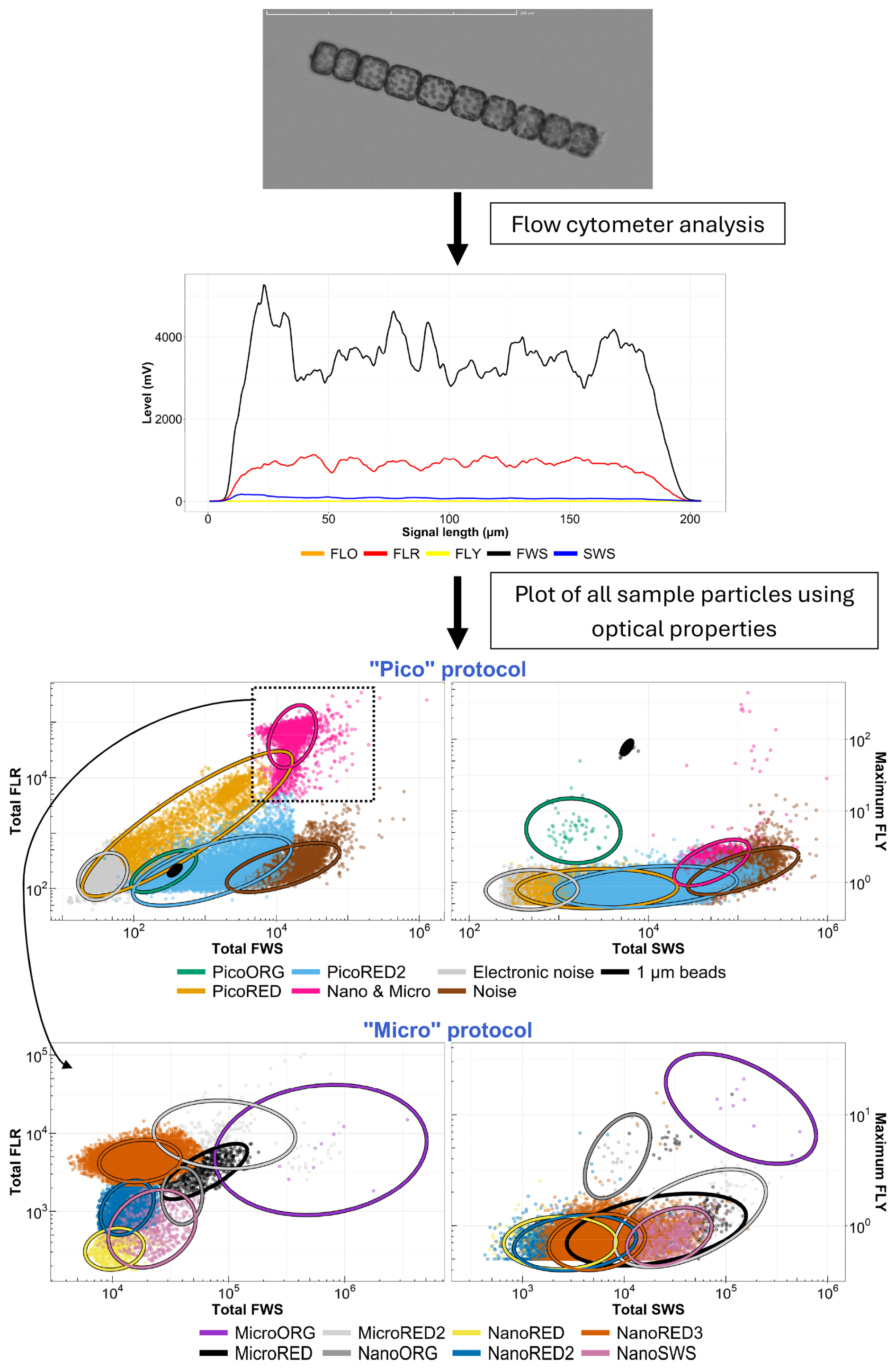
Figure 3 Diagram of the principle of the automated pulse-shape-recording flow cytometer, from particles to cytograms. The top figure shows an example picture of a colonial diatom (Lauderia sp.) taken by the CytoSub. Its associated optical spectrum is shown below. The cytograms shown at the bottom of the figure are based on the properties of the optical features of all of the cells and colonies analyzed for a single sample, calculated from the optical signals recorded and assigned to a single cluster using an exclusive set function. The colored scatter points and ellipses (t-distribution confidence interval of 95 %) are shown as a gating example for these particles.

Three cytometry protocols were used in this study, each optimized for specific size ranges. The “Pico” protocol targets particles below 5 µm, while the “Micro” protocol captures particles above 5 µm. A third protocol, “Micro-Photos”, mirrors the Micro protocol but uses a lower sample flow rate to acquire precise images of particles that comprise the different nano- and micro-PFGs (phytoplankton functional groups; Thyssen et al., 2022). While not allowing for a definitive taxonomic identification at the species or complex level, these images can suggest a possible composition of dominant groups – particularly for micro- and nano-PFG clusters. This visual information is further supported by the analysis of pulse shapes, which provide an in silico image of cells and colonies across all of the clusters. In 2021, a single threshold (or trigger level) based on minimal FLR was applied for both protocols. In 2022, two detection thresholds were used during in situ measurements by MAREL Carnot with the CytoSub, using both SWS and FLR signals to capture the longer pulse shape. This adjustment does not affect measurements of PFG abundance or total phytoplankton abundance.

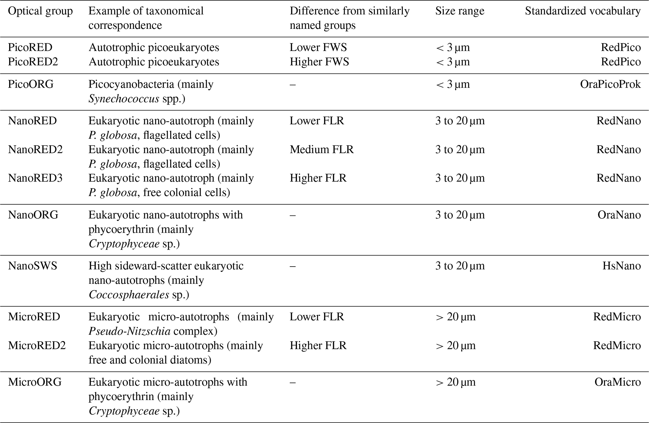
During this study, 11 PFGs were defined through manual clustering using the CytoClus 4 software. The bibliographic context of the study area involving the use of automated flow cytometry (Guiselin, 2010; Bonato et al., 2015; Louchart et al., 2020, 2024), sometimes in combination with complementary methods such as microscopy and the Micro-Photos protocol (based on photo identification), enabled us to interpret PFGs in terms of probable taxonomic equivalents, which were additionally related to the novel consensual nomenclature published in Thyssen et al. (2022) and detailed in Table 1. However, as our method was particularly atoxonomic for the smallest size classes where no photographs can be taken by the Micro-Photos protocol, it was not possible to provide definitive taxonomic identifications for the PicoRED groups. However, based on size (<3 µm) and fluorescence characteristics, the PicoRED groups likely include small picoeukaryotes such as Micromonas spp. or other similar prasinophytes (Not et al., 2004; Masquelier et al., 2011).

Table 1 Detailed glossary of the characterized PFGs. The taxonomical or optical interpretation of each group is based on determination by images and the literature. A particle belonging to a given group therefore has optical properties similar to those of the proposed optical equivalent even when it is uncertain that the observed particle corresponded to the given taxa (or attributed taxa). Thyssen et al. (2022) optical group common vocabulary equivalents and the associated size ranges are also provided.

To facilitate comparisons between the 2 study years, ordinal days (O_d) were standardized to the UTC+01:00 time zone (see Sect. 3.1).

2.3 Statistical analysis

2.3.1 Climatological baseline and definition of rare events

To assess the occurrence and intensity of rare environmental events (e.g., marine heat waves, desalination, and high-wind storms), we used a long-term baseline derived from high-frequency MAREL Carnot surface measurements collected between 2004 and 2023. The probability density functions of the parameters used are shown in Fig. 4. Percentile thresholds (e.g., the 90th, 95th, and 99th percentiles) were computed from this 20-year dataset and used to identify values considered anomalously high, as commonly done for time series rare event detection (e.g., Camuffo et al., 2020; Jamous and Marsooli, 2023; Hemming et al., 2024). This method provides a robust site-specific context for interpreting rare events.

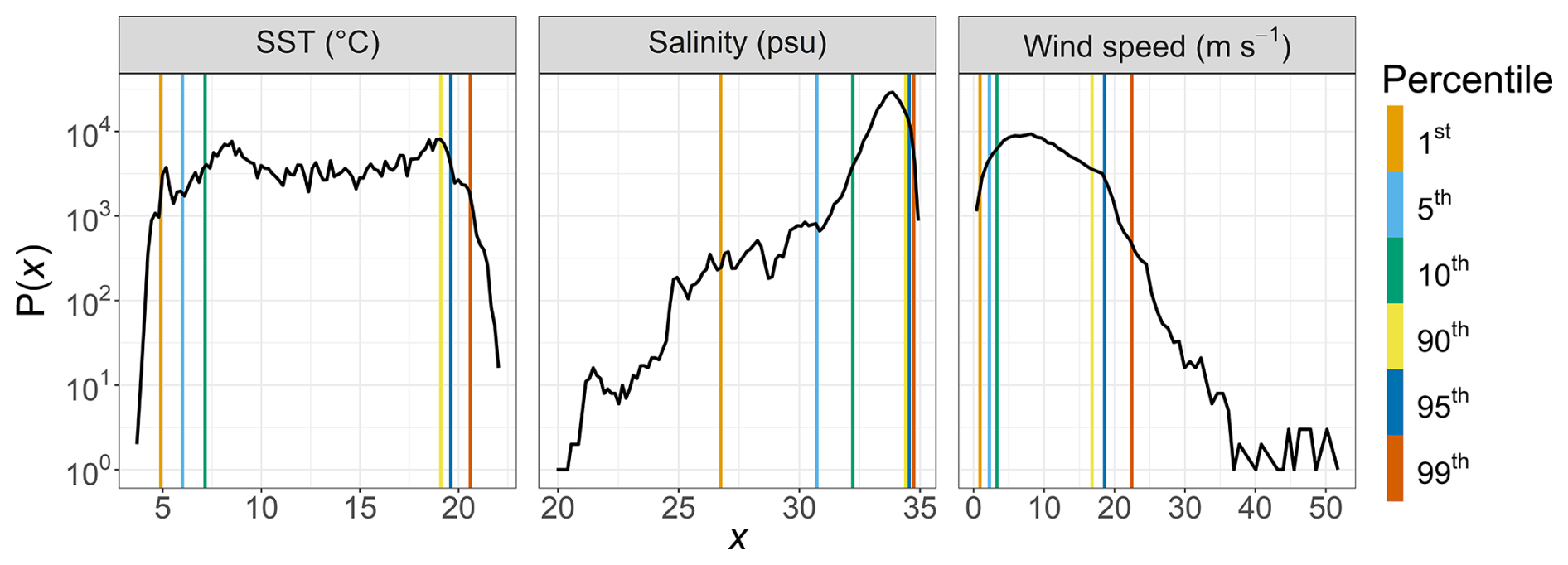
Figure 4 Probability density functions of MAREL Carnot SST (°C), salinity (psu), and wind speed (m s⁻¹) data recorded between 2004 and 2023. The colored dashed lines indicate the estimated percentiles for each time series.

2.3.2 Empirical mode decomposition and Lomb–Scargle periodogram (EMD–LSP) analysis

EMD was used to characterize the multiscale phytoplankton dynamics. This algorithm decomposes a time series X(t) into n intrinsic mode functions (IMFs) C_i(t) as described by Huang et al. (1998):

$$\begin{array}{}\text{(1)}& X\left(t\right)=\sum _{i=\mathrm{1}}^n{C}_i\left(t\right)+r_n\left(t\right).\end{array}$$

EMD works by first constructing upper and lower envelopes that connect the local maxima and minima of the time series. The mean of these envelopes defines the first zero-mean IMF C₁(t). This IMF is then subtracted from the original time series, and the process is repeated n times until a monotonic function r_n(t), representing the trend of the series, is obtained (Huang et al., 1998). This decomposition method allows a time series to be expressed as a sum of oscillating modes, each with a distinct characteristic scale, alongside a trend. EMD was previously used, for instance, to analyze phytoplankton dynamics in Lake Geneva (French–Swiss border) by Schmitt et al. (2013), where it was applied to study multiscale variability.

To determine the mean period of each IMF, we applied the LSP, a technique originally developed to analyze irregular astronomical time series (Lomb, 1976; Scargle, 1982) but applicable to biological time series (Ruf, 1999). The LSP evaluates various periodic patterns by fitting sine or cosine waves of different frequencies, amplitudes, and phases to the observed data. The most appropriate pattern, including its phase and amplitude, is identified by determining the frequency of the sinusoidal waveform that best describes the observed data. Only frequencies above 2f_min were retained based on the Nyquist–Shannon theorem. The mean period $\stackrel{\mathrm{‾}}{T_i}$ for each IMF was calculated using

$$\begin{array}{}\text{(2)}& \stackrel{\mathrm{‾}}{T_i}={\left({\displaystyle \frac{\underset{\mathrm{0}}{\overset{\mathrm{\infty }}{\int }}f{L}_i^{\mathrm{s}}\left(f\right)\mathrm{d}f}{\underset{\mathrm{0}}{\overset{\mathrm{\infty }}{\int }}{L}_i^{\mathrm{s}}\left(f\right)\mathrm{d}f}}\right)}^{-\mathrm{1}},\end{array}$$

where f is the frequency and $L_i^{\mathrm{s}}$ is the Lomb–Scargle spectrum of C_i(t). This method provides an energy-weighted calculation of the mean period (Huang et al., 1998, 2009). Additionally, the period of the maximum peak in the periodogram, T_max, was extracted. The code used to apply the EMD–LSP method is provided in the “Code and data availability” section.

To assess the contribution of each IMF to the total signal, we calculated the relative variance V_i=V(C_i). The variance lost $V_i^{\mathrm{lost}}$ after removing IMFs C₁ to C_i from the original signal was estimated using

$$\begin{array}{}\text{(3)}& V_i^{\mathrm{lost}}=\mathrm{100}\cdot {\displaystyle \frac{\sum _{k=\mathrm{1}}^i{V}_k}{\sum _{k=\mathrm{1}}^n{V}_k+V\left(r_n\right)}},\end{array}$$

where n is the total number of IMFs found for X(t). This calculation provides an estimate of the cumulative information loss across different timescales based on the periods of the different IMFs.

2.3.3 Shannon diversity index H^′

We applied the EMD–LSP method to the exponential value of the Shannon diversity index H^′ (Shannon, 1948) based on the cytometric optical communities:

$$\begin{array}{}\text{(4)}& H^{\prime }=-\sum _{i=\mathrm{1}}^S{p}_i{\log }_{\mathrm{2}}\left(p_i\right),\end{array}$$

where log ₂ is the binary logarithm, S is the number of communities, and p_i is the proportion of the community i in the entire ecosystem. The Shannon diversity index is widely used to characterize community diversity by considering both their richness (number of functional groups) and relative abundances (or relative FLR in our case) in a sample. It serves as an indicator of ecosystem health and can signal disturbance (Hill, 1973; Li, 1997, 2002). We examined the dynamics of its exponential form, known as Hill's diversity number of order 1 (Hill, 1973). This cytometric diversity index provides information about the non-taxonomic entropy of community assemblages and reflects the level of organization (in thermodynamic terms) of the ecosystem. The Shannon index dynamics capture how quickly the functional structure of a part of the ecosystem can change, as cytometric groups can be considered functional groups based on optical features as proxies of size, granulosity, and pigment content (Le Quéré et al., 2005; Fontana and Pomati, 2014; Fragoso et al., 2019; Fuchs et al., 2022; Louchart et al., 2024).

Shannon entropy is fundamental in phytoplankton ecology as it determines the community structure and can therefore be linked to the environmental conditions. It was previously applied to functional groups in other studies (e.g., Sun and Wang, 2021). The binary logarithm was used in Eq. (4) to express the measure in bits and to ensure comparability with previous ecological studies based on functional traits (e.g., Sun and Wang, 2021).

Here, we applied the EMD–LSP analysis to the time series of exp (H^′) to explore the variability in the arrangement of communities over multiple timescales. The aim was to account for its multiscale dynamics, spanning hours to days, and to understand the dynamic shifts in community assemblage.

3 Results

3.1 Phytoplankton phenologies

The abundance and FLR data (both total and per optically defined PFG) are shown in absolute values in Fig. 5 and in relative values in Fig. 6. First, it is important to note that these time series are incomplete. This results from technical failures that occurred during the deployments.

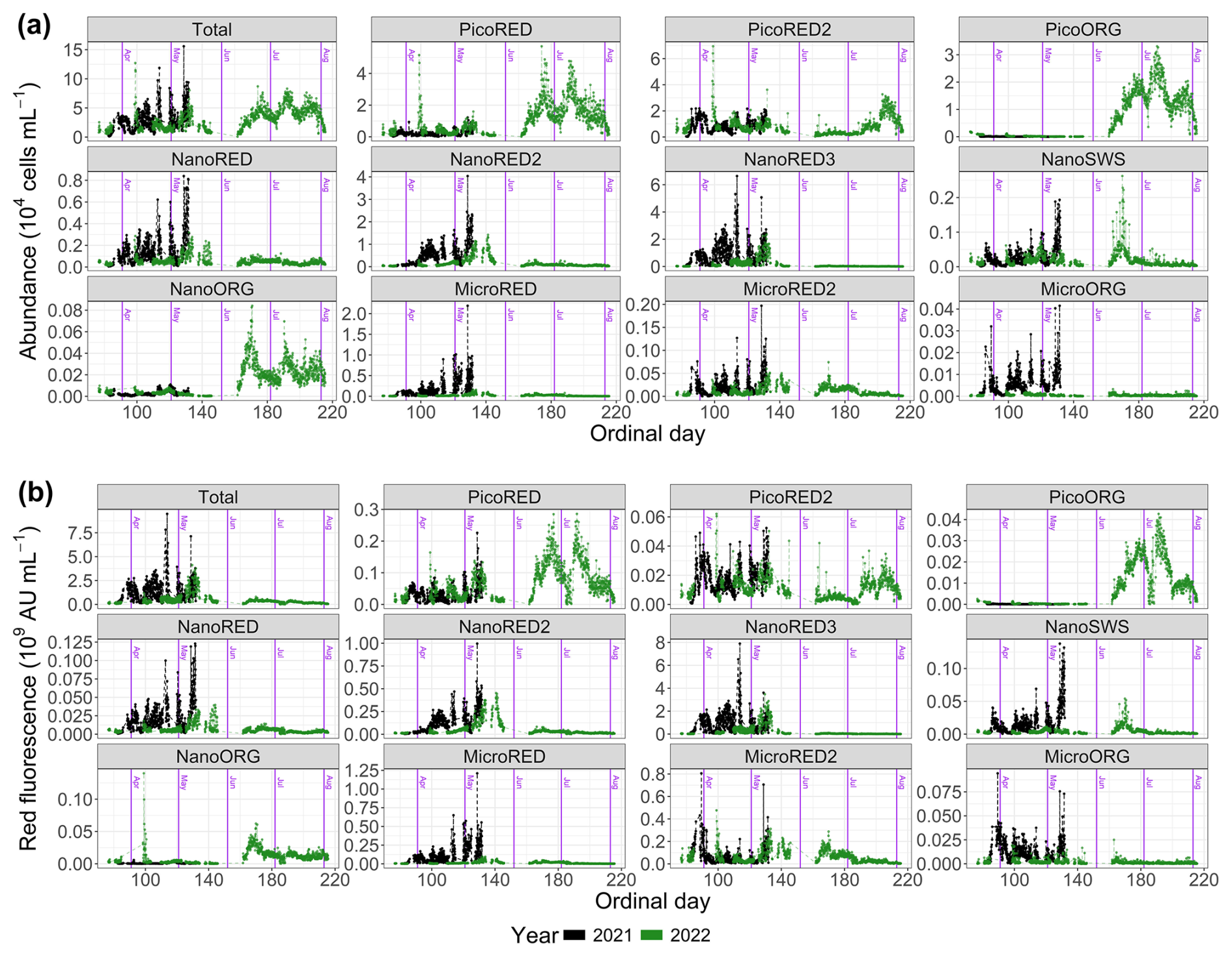
Figure 5 Phytoplankton data recorded with the automated flow cytometer (CytoSub) for each sampled ordinal day: (a) phytoplankton abundance and (b) phytoplanktonic red fluorescence (proxy of chlorophyll a expressed in arbitrary units per milliliter; AU). These data are represented in total values and per optically discriminated PFG. The black line and dots represent 2021 data, and the green line and dots represent 2022 data. The purple vertical lines indicate the start of each month.

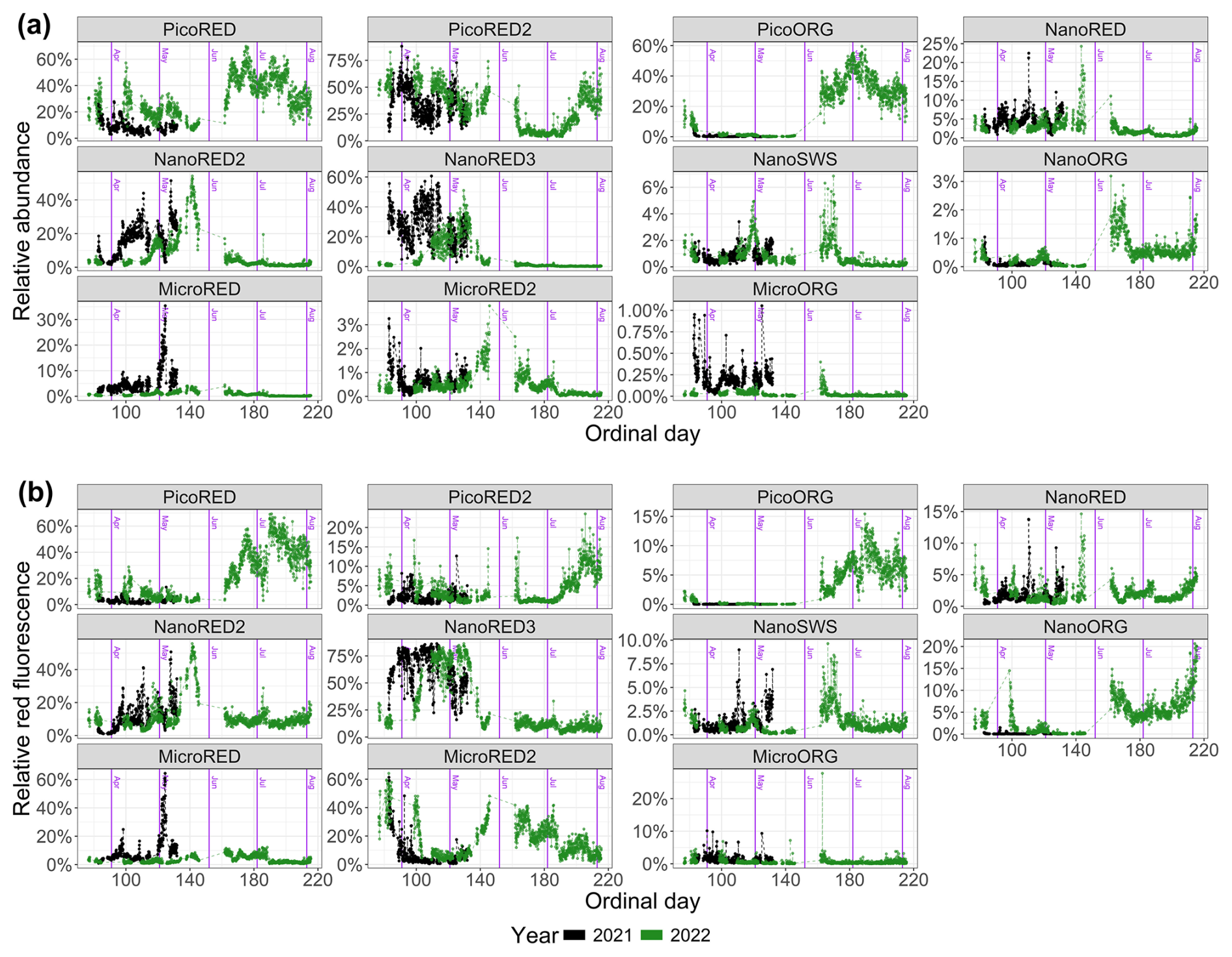
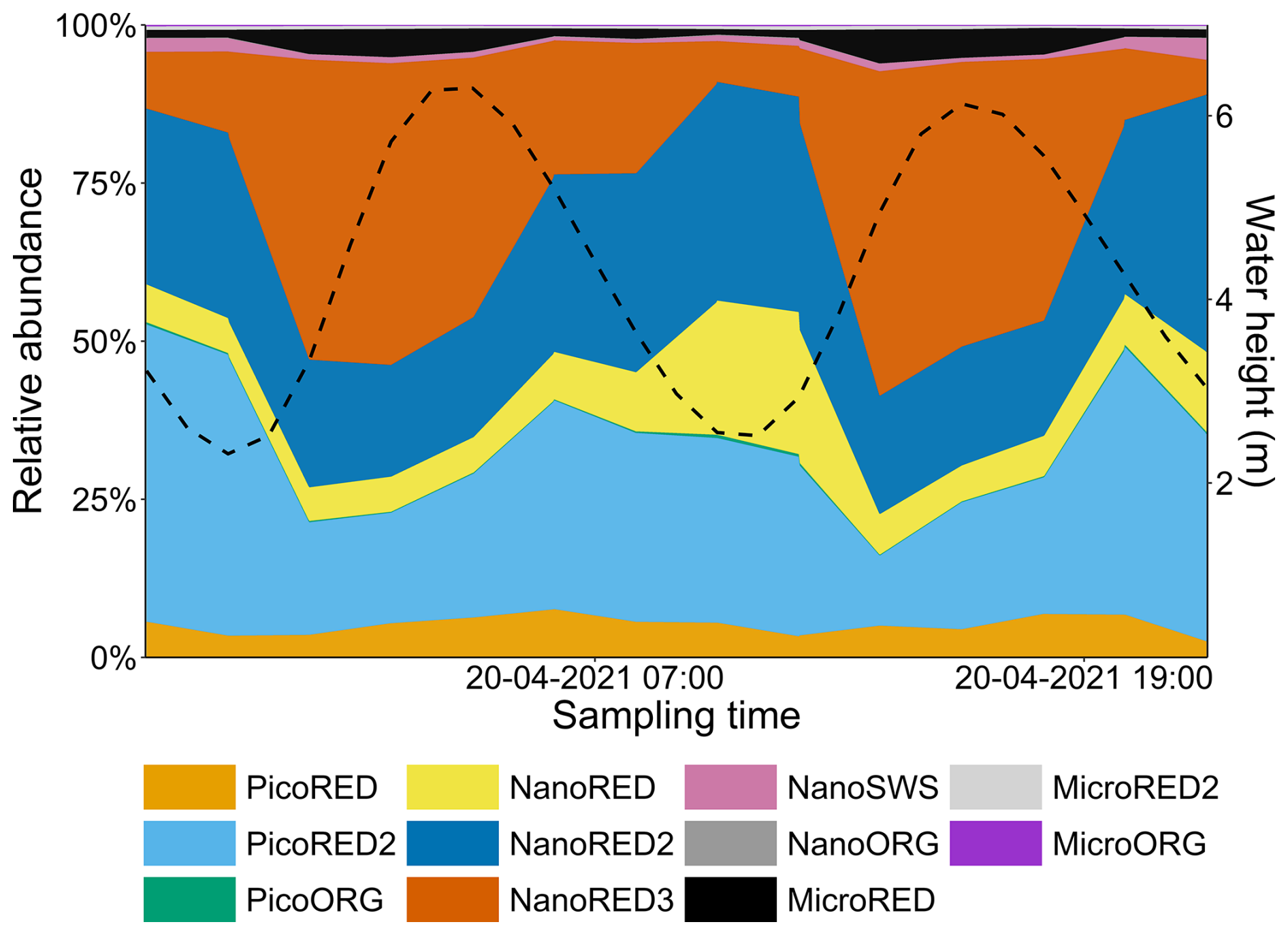
Figure 6 Phytoplankton data recorded for each group with the automated CytoSub for each sampled ordinal day: (a) PFG relative abundance and (b) PFG relative red fluorescence (proxy of chlorophyll a). The relative values of each group are computed as the ratio of the group's value to the total sum across all of the groups. The black line and dots represent 2021 data, and the green line and dots represent 2022 data. The purple vertical lines indicate the start of each month. Another representation of these results is proposed in Appendix C.

3.1.1 2021 deployment

The dynamics of the 2021 spring bloom on a seasonal scale can be divided into three distinct phases. At the start of the measurement series (O_d=82), the PicoRED2 group dominated, increasing from 8 % to 63 % of the total abundance between 24 and 26 March (O_d=83 and O_d=85). During this period ($J_{\mathrm{d}}\in [\mathrm{82};\mathrm{96}]$), the total abundance ranged from 0.12×10⁴ to 4.1×10⁴ cells per milliliter (Fig. 5a). The second phase began on 7 April (O_d=97), marked by the predominance of the NanoRED groups. These groups, initially dominant at the start of the study period, became the majority again, with a mean contribution of 58.5±11.3 % for $J_{\mathrm{d}}\in [\mathrm{97};\mathrm{121}]$. The total abundance during this phase ranged from 0.47×10⁴ to 11.87×10⁴ cells per milliliter (Fig. 5a). Notably, the contribution of this group to the total phytoplankton abundance fluctuated, with periods of high relative abundance coinciding with local maxima in the total abundance, followed by brief declines. Hourly fluctuations were also observed, driven by rare events in early May, which will be discussed in Sect. 3.2. Towards the end of the time series, the contribution of the NanoRED2 group to the total abundance increased (12.8 % above the average for its associated PFG time series), while that of the NanoRED3 group decreased (5.9 % below its average).

In terms of FLR (a proxy for chlorophyll-a biomass), a clear seasonal dynamic was observed. The MicroRED2 group was well-represented at the start of the bloom, spanning approximately 23 to 27 March (O_d=82 to O_d=86). Its contribution gradually declined through the beginning of April. This pattern may correspond to the initial diatom bloom, where the high FLR values reflect the metabolic activity of these cells. These high FLR values per cell may also reflect photo-acclimation to low light at the beginning of the blooming period (Houliez et al., 2013). As the season progressed, the NanoRED2 and NanoRED3 groups dominated the FLR time series, with rapid alternations in their relative importance signaling shifts in both community assemblage and physiological state. The peak in FLR was recorded on 24 April (O_d=114), coinciding with the core of the NanoRED bloom. This period, traditionally dominated by Phaeocystis globosa, saw significant representation of the NanoRED2 and NanoRED3 groups, and the associated increase in FLR indicates higher physiological activity during this phase. Towards the end of the bloom, starting on 7 May (O_d=127), the NanoRED2 group became increasingly prominent in contributing to the total fluorescence. This pattern aligns with abundance data, where NanoRED2 accounted for 28.8±6.0 % of the cumulative total abundance, peaking at 51.4 % on 8 May. The rise in FLR from NanoRED2 suggests enhanced metabolic processes and productivity in this group.

3.1.2 2022 deployment

The dynamics of the 2022 spring bloom can be divided into several phases. The first phase was dominated by the PicoRED groups, which accounted for 83.4±7.7 % of the total abundance during $J_{\mathrm{d}}\in [\mathrm{76};\mathrm{100})$, with a peak of 12×10⁴ cells per milliliter recorded on 9 April (O_d=99). In addition, the PicoORG group contributed on average 7 % between 23 and 27 March (O_d=82 and 86) to the total abundance. From 10 April (O_d=100), an increase in the NanoRED groups' total and relative abundances likely marked the onset of the P. globosa bloom. Between 5 and 27 May (O_d=125 to O_d=147), their relative abundance averaged 45.8±10.0 %, with absolute values ranging from 0.6×10⁴ to 8.0×10⁴ cells per milliliter. A succession was observed: NanoRED3 dominated between 6 and 16 May (O_d=126 to O_d=136), followed by NanoRED2 from 17 to 26 May (O_d=137 to O_d=146). Finally, from 10 June (O_d=161), blooms of PicoRED and PicoORG (Synechococcus spp.), NanoORG (Cryptophyceae), and NanoSWS (Coccolithophoridae) marked the last phase. After 10 July (O_d=191), the abundance of the PicoRED2 group also increased.

The dynamics of FLR in 2022 exhibited a distinct phenology compared to the 2021 bloom. Initially, the phytoplankton community was progressively dominated by the MicroRED2 group (mainly diatoms, as autotrophic dinoflagellates occur at very low abundance in the EEC during this period; Gómez and Souissi, 2007; Schapira et al., 2008; Lefebvre et al., 2011; Hubert et al., 2025b), which accounted for approximately 65 % of the total fluorescence on 23 March (O_d=82; Fig. 6b). This dominance persisted until 12 April (O_d=102). Subsequently, the NanoRED3 group became predominant, culminating in the peak FLR of the bloom on 10 May (O_d=130). This period coincided with the delayed P. globosa spring bloom, which occurred later than in 2021. From 6 May (O_d=126), the NanoRED2 group gained in prominence, ultimately becoming the most fluorescent group alongside the MicroRED2 group by 21 May (O_d=141). A notable increase in the MicroRED2 group's contribution to total fluorescence was observed through 26 May (O_d=146). In the final phase, starting on 10 June (O_d=161), the NanoSWS and NanoORG groups showed increased contributions to total fluorescence, although this occurred during a period of very low overall FLR values (Fig. 5b).

3.2 Rare events recorded

Four rare events were recorded during these two sampling periods: two with sharp wind increases, one desalination event (brackish water inputs), and one heat wave event (Fig. 7).

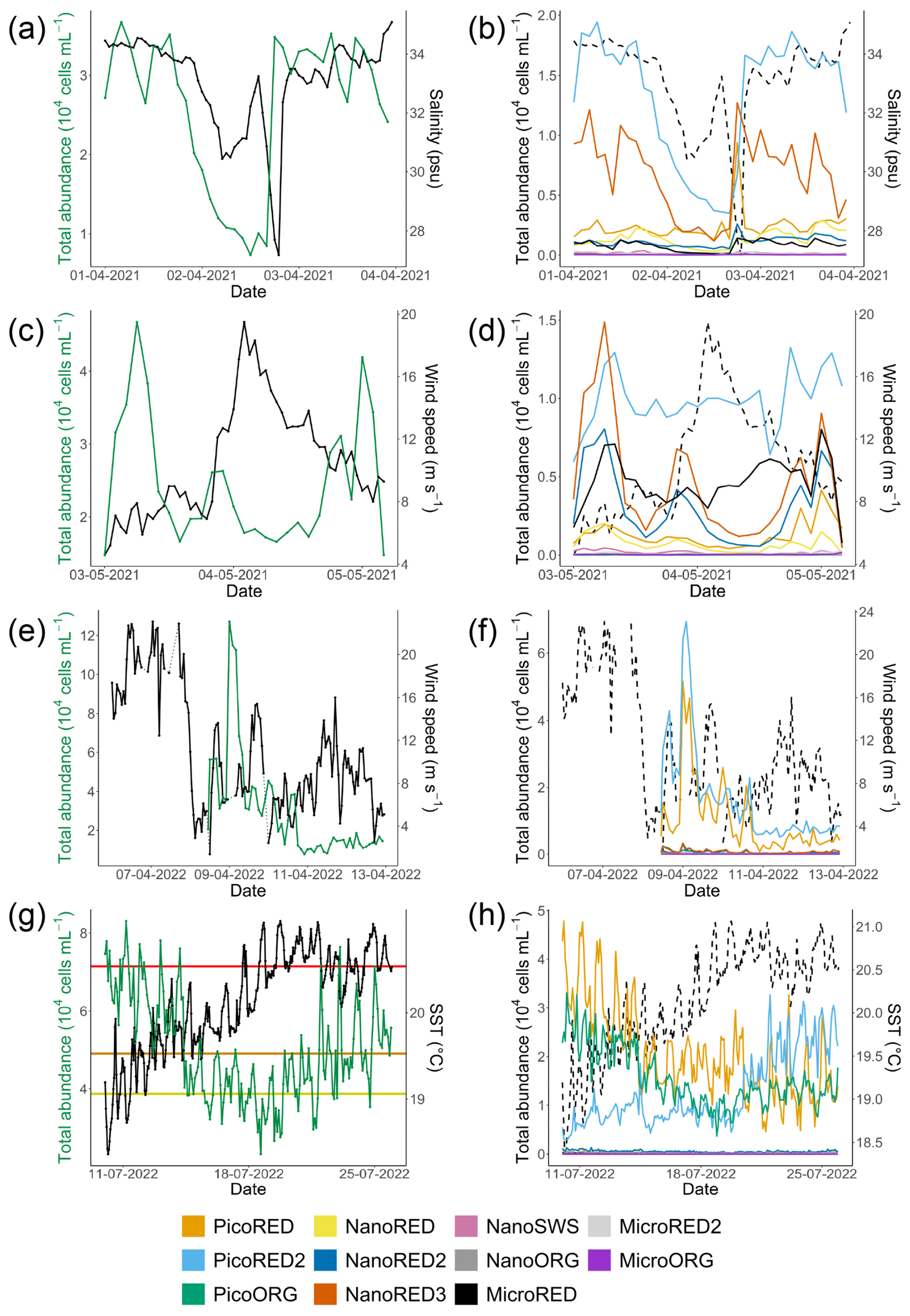
Figure 7 Examples of rare events recorded at the MAREL Carnot station during the study: (a, b) a desalination event in April 2021, (c, d) a high-wind-speed period in May 2021, (e, f) a strong-wind period in April 2022, and (g, h) a high-SST event (heat wave) in July 2022. Each of the corresponding parameters is shown on the second y axis (right axis) as a solid black line in the (a, c, e, g) left-hand figures and as a dotted line in the (b, d, f, h) right-hand figures. The absolute total abundances are given in the left-hand column (a, c, e, g; green line), and the absolute abundances for each phytoplankton group are given in the right-hand column (b, d, f, h; colored lines). The three horizontal lines of panel (g) represent the 90 % (yellow), 95 % (orange), and 99 % (red) percentiles of the SST observations of the MAREL Carnot station between 24 March 2004 and 30 September 2023. The abiotic data (salinity, SST, and wind speed) presented here come from (a–b, e–h) the MAREL Carnot station and (c, d) Météo-France (Boulogne-sur-Mer station).

The desalination event occurred between 1 and 4 April 2021 (Fig. 7a and b), with salinity values falling below the 5th percentile (30.73 psu) of the MAREL Carnot salinity dataset (from 2004 to 2023, n=325 699 observations). During the initial phase of this event, the total phytoplankton abundance decreased, driven primarily by declines in the PicoRED2 and NanoRED3 groups. Subsequently, salinity values dropped even further (<28 psu), coinciding with peaks in the abundances of the PicoRED, NanoRED, and MicroRED groups. Notably, the NanoRED3 group exhibited a more rapid change in abundance compared to PicoRED2 during the salinity decline.

The second event observed in 2021 was a breeze with wind (coming from the southwest, with a direction between 200 and 260° relative to true north; see Appendix D) speeds ranging from 8 to 20 m s⁻¹ (Fig. 7c and d), exceeding the 90th percentile of the MAREL Carnot wind data (16.8 m s⁻¹; from 2004 to 2023, n=151 663 observations). During this event, the total phytoplankton abundance decreased sharply, particularly during the initial rise in wind speed on 3 May, and remained low through the larger peak on 4 May. All of the groups followed the trend of total abundance decline, except for PicoRED2 and MicroRED, which dominated both total abundance and fluorescence during this period. After the main wind episode, the abundance of NanoRED2 and NanoRED3 increased, accompanied by high chlorophyll fluorescence, with MicroRED representing more than 60 % of the total fluorescence (Fig. 6b), although the overall fluorescence remained low (between 0.5×10⁹ and 0.6×10⁹ AU mL⁻¹ on 3 May).

The third event, a high-wind storm (storm Diego) in April 2022 (Fig. 7e and f), was marked by a peak in phytoplankton abundance on 9 April. Unfortunately, wind data for this peak were unavailable due to a power outage caused by the severe weather conditions. However, the data recorded before and after the cutoff show a change in wind direction at the peak, with winds shifting from southwesterly to northeasterly for about 1 d (see Appendix D). The PicoRED groups were particularly affected during this event, with observed peaks in their abundance that seemed linked to the wind speeds. In terms of fluorescence, this event appeared to favor the NanoORG group, which reached a relative fluorescence of 15 % (Fig. 6b) during a fluorescence peak, with absolute values close to 1.2×10⁹ AU mL⁻¹ (Fig. 5b).

The final event was a marine heat wave (Fig. 7g and h) marked by warm water and high air temperatures in Boulogne-sur-Mer between 15 and 20 July 2022, with the highest air temperature recorded on 19 July (temperature in a Stevenson screen equal to 39.8 °C according to the Météo-France data). This event qualifies as a marine heat wave, as the SST reached the 90th percentile (estimated from the MAREL Carnot data from 2004 to 2023, n=339 137 observations) for at least 5 d (Hobday et al., 2016). We did not have 30 years of data as recommended to define the marine heat wave threshold, but this event qualification was supported by other studies in the same study location showing an intense activity of marine heat waves during the summer of 2022 in the English Channel (Simon et al., 2023). During this period, phytoplankton abundances decreased as the SST increased, from the 90th (19.06 °C) to 95th (19.53 °C) and 99th (20.54 °C) percentiles recorded since 2004. This decline was particularly evident in the PicoRED and PicoORG groups, which were among the most dominant during this period. PicoORG abundance, for example, halved during the event, and its dynamics showed a strong negative correlation with SST (Pearson $r=-\mathrm{0.78}$ and p value < $\mathrm{2.2}\times {\mathrm{10}}^{-\mathrm{16}}$) between 10 and 20 July. After 21 July, both PicoORG and PicoRED stabilized as SST plateaued. In contrast, PicoRED2 abundance increased during and after the SST peak.

3.3 EMD–LSP

3.3.1 A first example: 2021 abundance time series

The results obtained with EMD–LSP analysis of the 2021 abundance time series were arbitrarily chosen here for presentation in detail in order to provide an example of the interpretation of the EMD–LSP analysis results. Nevertheless, all results for the other time series are presented in Table 2.

Table 2 Indicators estimated from EMD–LSP for each IMF C_i(t) of the abundance, red fluorescence (FLR), and Shannon index H^′ time series of 2021 and 2022: the period of the maximum peak of the LSP T_max (d), the mean period $\stackrel{\mathrm{‾}}{T_i}$ (d), the loss of explained variance in the time series after removing the i first IMFs $V_i^{\mathrm{lost}}$ (%), and the γ value for which $\stackrel{\mathrm{‾}}{T_i}\sim {\mathit{\gamma }}^i$.

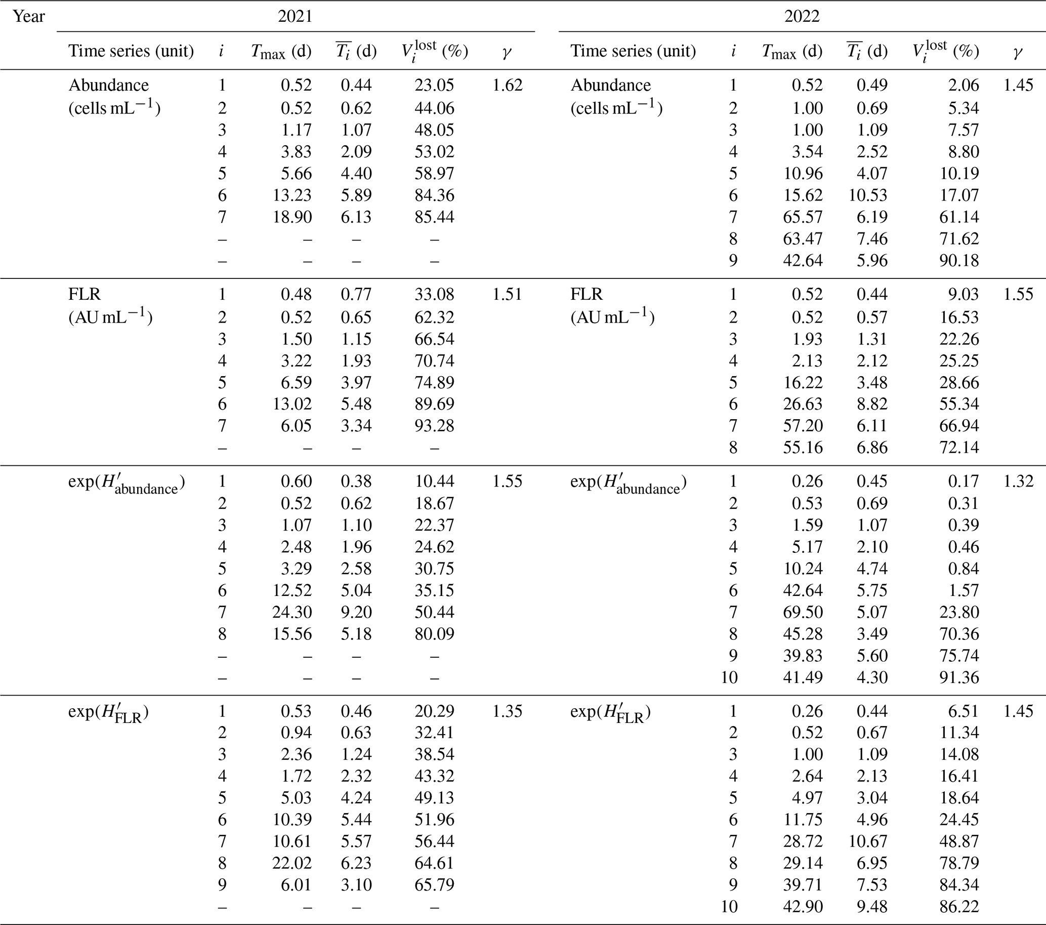
For this case, seven IMFs were identified, with peak periods ranging from approximately 12.48 h to 18.9 d (Fig. 8). These periods (T_max; see Table 2) corresponded to the highest peaks in their respective LSPs. The mean periods of these IMFs ranged from 10.6 h to 6.1 d (Fig. 9a). The first IMF, C₁, had a mean period of 10.6 h, a peak at 12.4 h, and an additional peak at around 6 h. This IMF likely corresponds to the current inversion during tides (Jouanneau et al., 2013). The second IMF represents the tidal mode with a mean period of 14.9 h and a peak near 12.4 h. The third IMF, C₃, corresponds to two tidal cycles ($\stackrel{\mathrm{‾}}{T_{\mathrm{3}}}=\mathrm{1.07}$ d), while the fourth and fifth IMFs, C₄ and C₅, are likely related to tidal cycle impacts at different timescales ($\stackrel{\mathrm{‾}}{T_{\mathrm{4}}}=\mathrm{2.09}$ d and $\stackrel{\mathrm{‾}}{T_{\mathrm{5}}}=\mathrm{4.40}$ d). The final two IMFs, C₆ and C₇, align with the periodicity of the neap–spring tide cycle, with periods near the semi-lunar cycle (T_max=13.2 and 18.9 d, respectively). The residual dynamics showed an overall increase in total phytoplankton abundance during the bloom period, with fluctuations following the lunar cycle. Peaks in abundance corresponded to spring tides, while troughs aligned with neap tides.

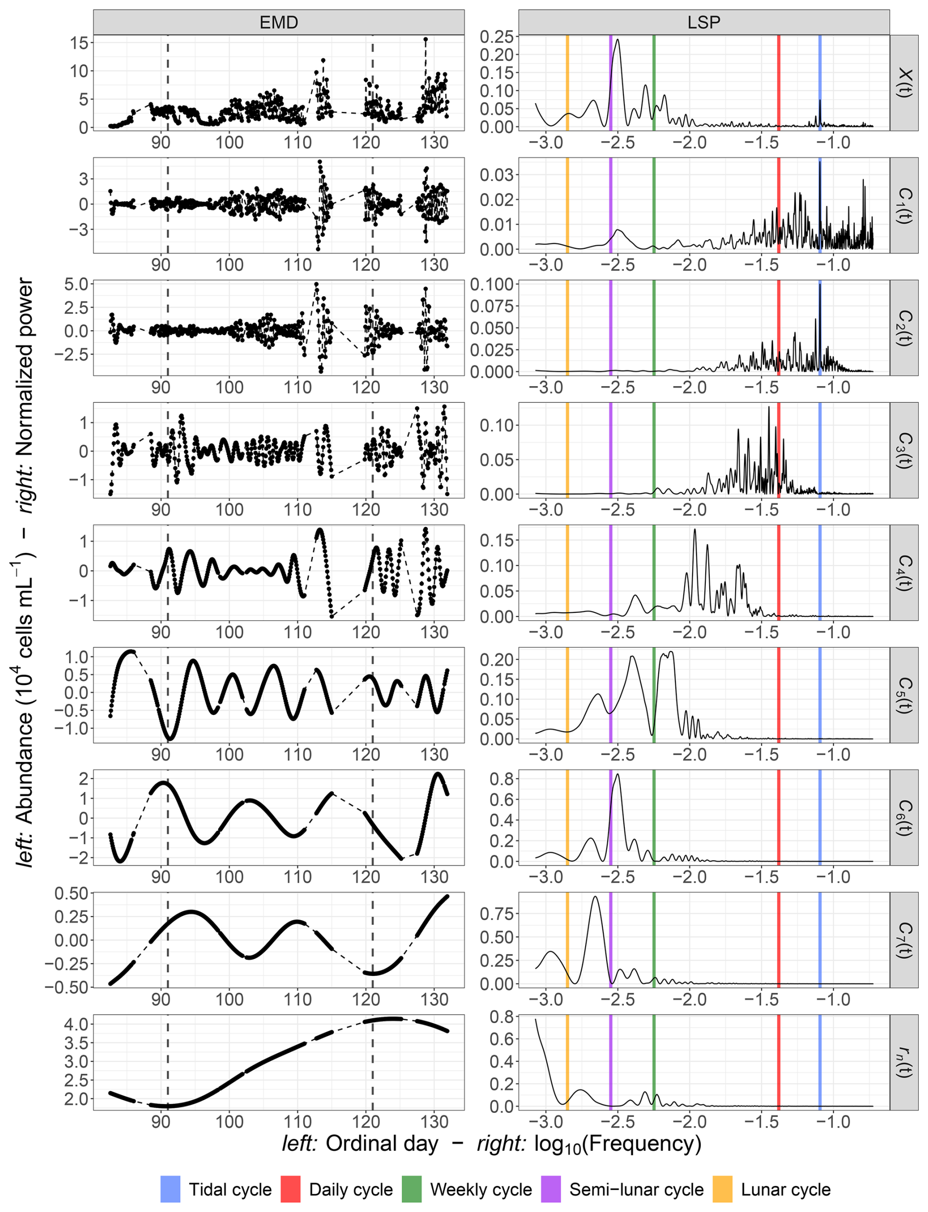
Figure 8 Decomposition of the 2021 total phytoplankton abundance data using empirical mode decomposition (EMD; left part) and the associated Lomb–Scargle periodograms (LSPs; right part) for the raw time series X(t), for each IMF C_i(t) and for the residual r_n(t). The EMD x axis represents the ordinal days, and the y axis represents the abundance values (10⁴ cells per milliliter). The LSP x axis represents the decimal logarithm (log ₁₀) of the frequency (h⁻¹), and the y axis represents the normalized power. The gray dashed lines (left column) represent the beginning of April and May 2021.

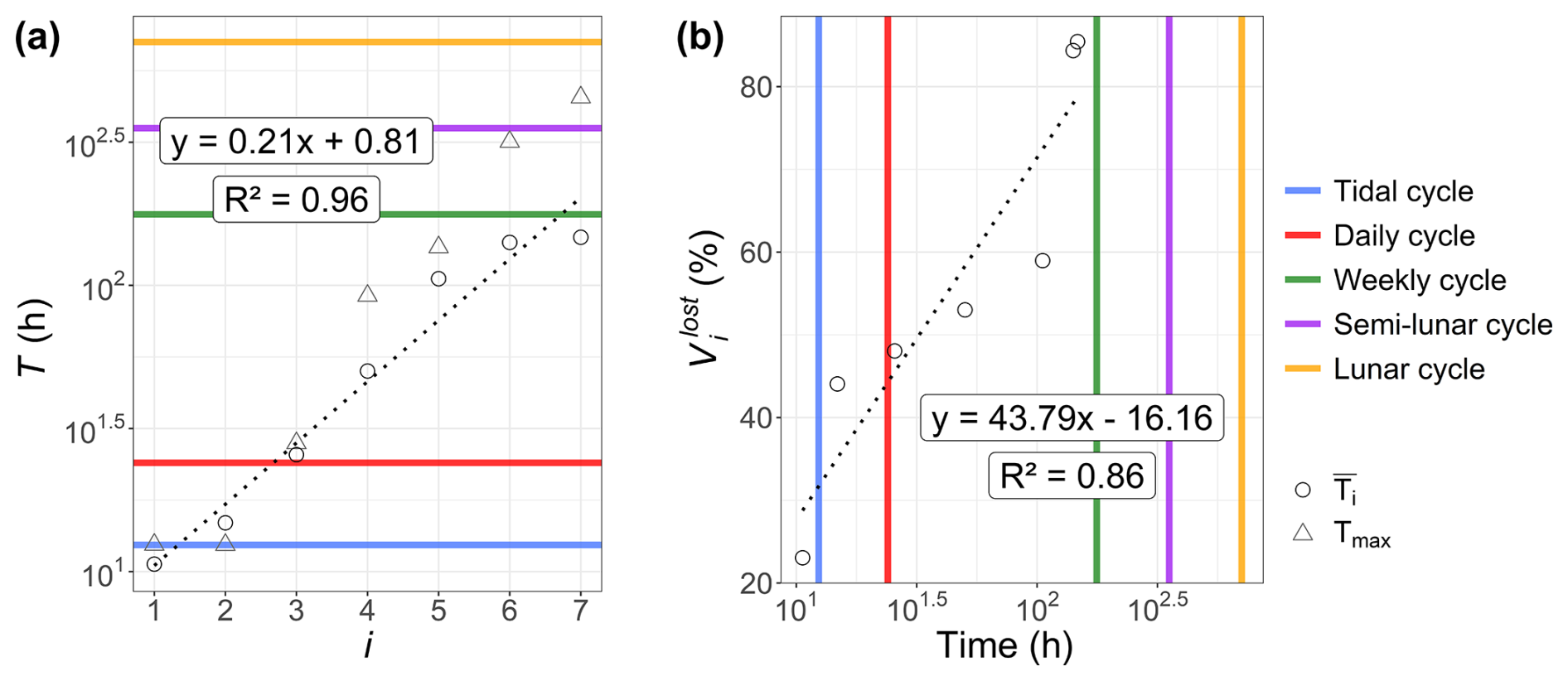
Figure 9 Results obtained from the EMD–LSP analysis for the 2021 phytoplankton abundance time series: (a) the mean period ($\stackrel{\mathrm{‾}}{T_i}$) and maximum peak period (T_max) of each IMF C_i(t) and (b) the percentage of variance explained for different timescales based on the mean periods of these IMFs. The black dashed lines represent the estimated linear regressions. The associated formula and coefficient of determination R² are displayed in the respective figures.

Notably, the periods of the different IMFs follow a power law: $\stackrel{\mathrm{‾}}{T_i}\sim {\mathit{\gamma }}^i$. The exponent γ was found to be 1.62, which is lower than the value of 2 typically observed for fractional Gaussian noise (Flandrin et al., 2004; Flandrin and Gonçalvès, 2004) or turbulent time series (Huang et al., 2008). This indicates that the period of each mode is approximately 1.62 times longer than that of the preceding mode. The loss of variance, $V_i^{\mathrm{lost}}$, is shown in Fig. 9b for the first example, illustrating the loss of information after removing each IMF from the raw abundance signal. The explained variance decreases with the removal of each IMF, with the loss following a logarithmic pattern: $V_i^{\mathrm{lost}}\sim \mathrm{43.79}\cdot {\log }_{\mathrm{10}}\left(\stackrel{\mathrm{‾}}{T_i}\right)$.

3.3.2 Abundance and FLR

The EMD–LSP results for all of the studied abundance and FLR time series are summarized in Table 2. Each abundance and FLR time series exhibited between 7 and 10 distinct IMFs, with mean periods ranging from approximately 9 h to 11 d. Notably, the variance loss increased sharply with the different modes, particularly for the 2021 abundance and FLR time series, where tidal modes accounted for at least 44 % of the total variance. The 2022 tidal modes were less important in the total variance of the time series, with values ranging between 5 % and 17 %. The γ values ranged from 1.45 to 1.62, lower than the value of 2 typically found in turbulent and Gaussian time series, indicating the presence of many high-frequency modes.

Overall, a significant proportion of the variability was lost quickly, with at least 72 % of the variance disappearing for time series without modes and with mean periods between 4 and 11 d. This suggests that most phytoplankton variability occurred at low timescales. Additionally, according to the Nyquist–Shannon theorem, fluctuations at frequencies f_e cannot be captured by sampling frequencies lower than $\mathrm{2}/f_e$. Thus, a time resolution of at least 5 h is necessary to avoid losing this high-frequency modal variability.

3.3.3 Link between phytoplankton dynamics and tidal forcing

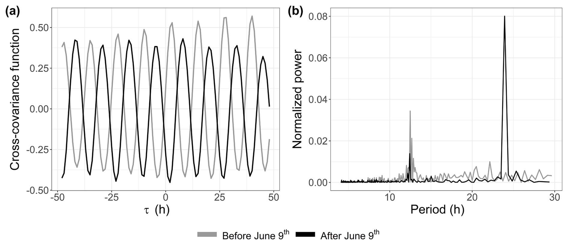
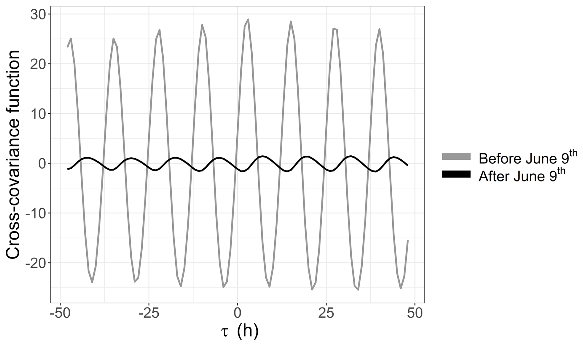
A link between the phytoplankton dynamics (abundance and FLR) and the tidal cycle was highlighted with EMD–LSP analysis (mostly for the 2021 time series). This link was investigated further through cross-correlation with the water height time series. This analysis revealed a shift in the short-timescale dynamics of phytoplankton abundance in 2022 occurring after 9 June (Fig. 10a). For the 2021 data (not shown here) and the early part of the 2022 data, phytoplankton abundance (and FLR; see Appendix B) showed a positive correlation with water height. However, after 9 June 2022, the relationship became negative. Furthermore, the LSP revealed a shift in dynamics before and after 9 June. A high peak was observed at 12 h before 9 June, which persisted but with reduced power after this date. A new peak appeared at 24 h, highlighting the changing temporal variability of the environmental forcing in phytoplankton communities (Fig. 10b). This illustrates the emergence or variation in the intensity of forcing effects in the time series of abundance and FLR, highlighting the nonlinearity of phytoplankton dynamics over time.

Figure 10 Short-timescale observations for the 2022 phytoplankton abundance data before and after 9 June: (a) cross-covariance functions between the water height data (REFMAR data; SHOM, 2024) and the abundance data and (b) Lomb–Scargle periodograms of the abundance data.

3.3.4 Shannon diversity index H^′

A difference was observed in the dynamics of the diversity index, exp (H^′), when calculated from abundance ($H_{\mathrm{abundance}}^{\prime }$; Fig. 11a) versus FLR ($H_{\mathrm{FLR}}^{\prime }$; Fig. 11b). In 2022, the diversity index based on abundance decreased after O_d=160 (9 June), while the FLR-based index increased during the same period (Fig. 11c). This shift can be attributed to the dominance of pico-organisms during the summer bloom, which have a lower chlorophyll-a content and, therefore, contribute less to the total FLR. In contrast, $H_{\mathrm{abundance}}^{\prime }$ peaked during the NanoRED bloom (Fig. 11a), while $H_{\mathrm{FLR}}^{\prime }$ showed an opposite trend (Fig. 11b).

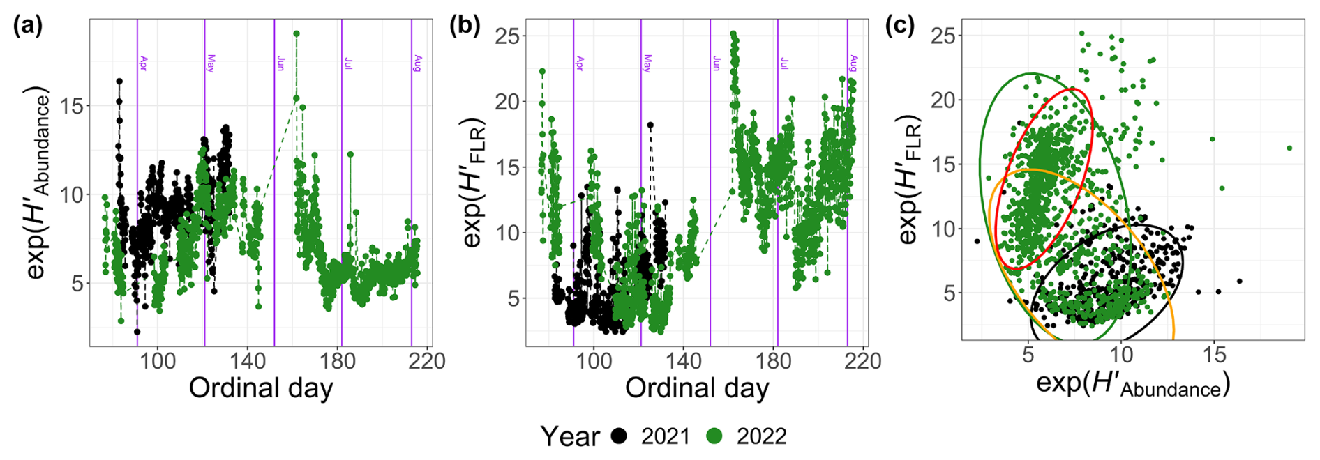
Figure 11 Exponential values of the Shannon index H^′ calculated for 2021 and 2022 based on (a) the abundance ($H_{\mathrm{abundance}}^{\prime }$), (b) the FLR ($H_{\mathrm{FLR}}^{\prime }$) as a function of the ordinal day, and (c) a comparison of these two quantities. The ellipses represent the t distributions with a 95 % confidence interval. The orange ellipse takes into account 2022 data before 9 June, and the red one takes into account those after 9 June.

The Shannon index time series exhibited similar IMFs to those observed for abundance and FLR, with notable high-frequency variations and the presence of tidal modes (T_max≃0.52 d). These tidal modes likely reflect the varying responses of different PFGs to tidal forces, with community assemblage evolving during each tidal cycle (Fig. 12). The γ values ranged from 1.32 to 1.55 (Table 2), indicating the dominance of high-frequency modes at short timescales, which accounted for at least 65 % of the variability. These findings underscore the multiscale dynamics of the system, with high-frequency variations playing a significant role in shaping phytoplankton community assemblages.

Figure 12 Relative abundance of each PFG (colored area) and water height (black dashed line; SHOM, 2024) between 19 and 21 April 2021.

4 Discussion

In this study, an automated flow cytometer was deployed at the MAREL Carnot fixed automated measuring station to monitor phytoplankton at high frequency. The goal was to observe and describe the variations in phytoplankton time series across several timescales, ranging from hourly events (e.g., rare events and tidal forcing) to monthly events (e.g., phenologies). It was hypothesized that these multiscale events influence phytoplankton communities.

4.1 Weekly-scale dynamics

In the spring of 2021, a significant bloom of NanoRED groups was observed, emerging phenologically in an environment where MicroRED2 (large diatoms and colonies) and PicoREDs (picoeukaryotes) dominated in terms of FLR and abundance, respectively. The increasing abundance of NanoRED groups was mostly due to the haptophyte P. globosa, which could be characterized by imaging (using the Micro-Photos protocol) and corroborated by previous studies (Rutten et al., 2005; Guiselin, 2010; Bonato et al., 2015). This phase corresponded to the onset of the P. globosa bloom, a phenomenon typical of the EEC (Breton et al., 2000, 2021, 2022) and frequently monitored due to its classification as a HAB (Lefebvre and Dezécache, 2020).

This phenological shift, with a transition from diatoms (MicroRED2) to P. globosa (NanoREDs), was also observed in 2022 and was previously documented in the study area (Breton et al., 2000; Guiselin, 2010; Grattepanche et al., 2011; Lefebvre et al., 2011; Hernández-Fariñas et al., 2014; Genitsaris et al., 2015; Lefebvre and Dezécache, 2020; Houliez et al., 2023). The P. globosa spring bloom is known to occur when abiotic conditions become favorable, such as nutrient availability and light conditions according to the literature (e.g., Gentilhomme and Lizon, 1997; Lancelot et al., 2011; Lefebvre et al., 2011; Lefebvre and Dezécache, 2020; Breton et al., 2022). More specifically, P. globosa became predominant following the depletion of Si(OH)₄ and ${\mathrm{PO}}_{\mathrm{4}}^{\mathrm{3}-}$ (Fig. 2), which were consumed during the diatom bloom, as observed in other studies (Karasiewicz et al., 2018).

The abundance of the MicroRED group was also notably high during the spring bloom of 2021. This group, composed of pennate diatoms optically similar to the Pseudo-Nitzschia complex (e.g., P. delicatissima, P. pungens, and P. seriata in this season; Delegrange et al., 2018), was confirmed through the Micro-Photos protocol. The presence of MicroREDs could be linked to the high abundance of P. globosa, as a commensal symbiotic relationship between these two species has been described (epibiosis; Sazhin et al., 2007).

A similar spring bloom of NanoREDs was observed in 2022, although it was less pronounced in terms of FLR compared to 2021. This difference in bloom intensity is also reflected in the post-bloom phase, with higher ammonium concentrations in 2021 suggesting more intense remineralization compared to 2022. This could be attributed to the longer persistence of nanoplankton and microplankton cells in 2021, which may have been facilitated by higher ${\mathrm{PO}}_{\mathrm{4}}^{\mathrm{3}-}$ concentrations during that year (Fig. 2). Moreover, limiting nutrients (${\mathrm{PO}}_{\mathrm{4}}^{\mathrm{3}-}$, Si(OH)₄, ${\mathrm{NO}}_{\mathrm{3}}^{-}$, and ${\mathrm{NO}}_{\mathrm{2}}^{-}$) were rapidly depleted at the onset of the bloom, consistent with the growth of diatoms (MicroRED2) and haptophytes (NanoREDs).

In 2022, the decline of the NanoRED bloom was evident, unlike in 2021, when measurements were ended earlier than in 2022. As the NanoRED bloom faded, other groups began to increase, including coccolithophorids (NanoSWS), cryptophytes (NanoORG), diatoms (MicroRED2) in terms of FLR, and particularly cyanobacteria (PicoORG) and chlorophyll picoeukaryotes (PicoREDs) in terms of abundance. The dominance of these smaller cells following the spring bloom can be explained by their higher competitiveness in nutrient-poor environments (Litchman et al., 2007). Similar successions have been observed in the region and are partly explained by the physicochemical conditions of the ecosystem (Bonato et al., 2016).

Furthermore, a succession between the NanoRED3 and NanoRED2 groups was also apparent at the end of the spring bloom (Fig. 13). As the abundance of NanoRED3 declined, NanoRED2 became more dominant for a period. This phenomenon, also observed at the end of the 2021 data recording (although less clearly), may reflect competition between different life stages of P. globosa (see Figs. 5 and 6). The flagellated form of P. globosa (NanoRED2) is more competitive in nutrient-limited environments compared to its colonial cell form (NanoRED3; Rousseau et al., 1994; Peperzak et al., 2000). As nutrients were consumed, the abundant form of this haptophyte shifted, revealing a long-term phenology driven by the gradual depletion of nutrient stocks during the spring and early summer (visible in Fig. 2; Gentilhomme and Lizon, 1997; Lancelot et al., 2011; Lefebvre et al., 2011).

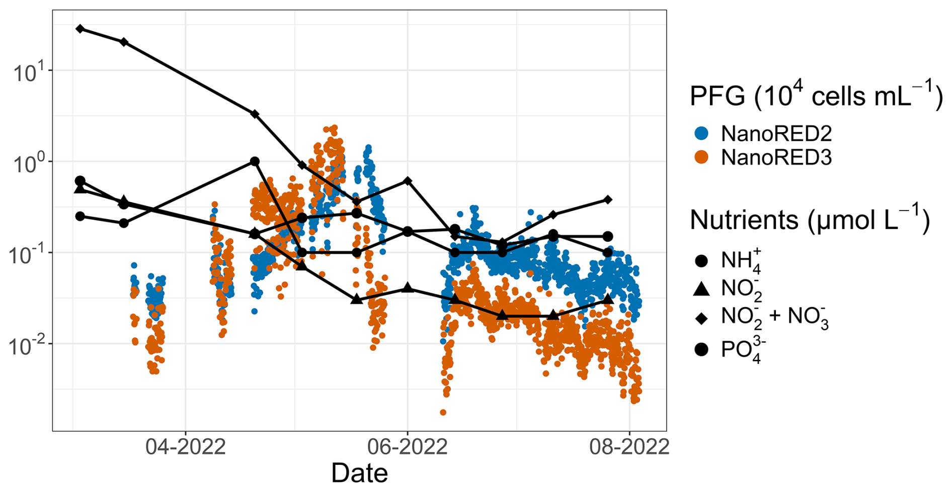
Figure 13 SRN nutrient data (Lefebvre et al., 2024) for the 2022 study period. The NanoRED2 and NanoRED3 2022 abundance data are represented by the colored dots. The logarithmic scale for the y axis was chosen for visualization purposes.

4.2 Rare events

High-frequency studies enable the detection of rapid and intense events that cannot be captured with low-frequency sampling typical of long-term monitoring networks. These events can have significant ecological impacts, as different phytoplankton communities respond differently to environmental changes. This was evident during two high-wind-speed events, which had contrasting effects on phytoplankton abundance.

In one instance, a strong-wind event between 3 and 6 May 2021 promoted the dominance of the MicroRED PFG (comprising the Pseudo-Nitzschia complex). During this period, all NanoRED groups decreased, while MicroRED groups increased. This shift could be explained by the resuspension of cells that had previously settled, supported by the observed increase in turbidity during this time (based on MAREL Carnot data not shown here). Additionally, the breakdown of P. globosa colonies, possibly due to their commensal relationship with MicroRED groups (Sazhin et al., 2007), could have contributed to this increase.

Following the wind event, NanoRED groups went up, likely due to the release of P. globosa colonial forms. Interestingly, pico-organisms (PicoRED and PicoRED2) did not appear to be significantly affected by this storm. In contrast, a high-wind-speed event in 2022 triggered a peak in the abundance of PicoRED groups. The difference in the effects of the two events may be attributed to the wind direction: during the 2021 event, the wind was blowing from 225° (southwest), while during the 2022 event the wind came from 350° (north-northwest) shortly before the PicoREDs abundance peak (as the weather station data ceased on 9 April). Wind direction is an important factor in particle transport in the harbor, and this shift could explain the contrasting responses of the phytoplankton groups (Jouanneau et al., 2013).

Additionally, the marine heat wave and low-salinity events highlighted in Sect. 3.2 induced different responses among phytoplankton communities, with significant shifts in the assemblages occurring over just a few hours. For instance, the PicoRED2 PFG appeared to be favored during the marine heat wave compared to other picoplankton groups. During the 2021 low-salinity event, two distinct peaks of low salinity were observed on the same day, yet the communities responded differently at each peak. These observations underscore the complexity and nonlinearity of phytoplankton community responses to rare events, even within the same area. Further high-frequency observations are crucial for fully understanding the effects of such events on pelagic phytoplankton ecosystems, as emphasized by previous studies (e.g., Barrillon et al., 2023; Röthig et al., 2023).

4.3 High-frequency multiscale dynamics

The time series analyzed revealed a multiscale dynamic ranging from hours to several days, with high-frequency fluctuations (9 h to 11 d) explaining at least 65 % of the total phytoplankton variance. Notably, tidal modes contributed significantly to the phytoplankton dynamics, as observed in other regions for chlorophyll a (Blauw et al., 2012). The high tidal range in our study area, along with temporal heterogeneity and patchiness of phytoplankton, likely drives this variability in total abundance and total FLR (Seuront et al., 1996; Seuront, 2005). Additionally, the neap–spring tidal cycle influenced the data, with an increased tidal range during spring tides amplifying the phytoplankton variability. This effect is linked to the coastal river's structure, where a vertical front during spring tides limits exchanges between coastal and offshore waters, isolating phytoplankton blooms near the coast, especially in a westerly wind regime.

High-frequency dynamics also impacted community assemblage, with shifts observable in the Shannon diversity index (estimated for communities), reflecting changes at multiple ecological scales. The tidal mode influenced this index, representing up to 20 % of the total variability and highlighting the diverse influence of hydrological forcing on different PFGs. This indicates that multiscale dynamics and high-frequency fluctuations affect the phytoplankton ecology at the community level.

Furthermore, high-frequency forcing effects were not stable over time. After 9 June 2022, a shift was observed in the relationship between phytoplankton abundance and water height, alongside the emergence of a new 24 h periodicity. This change could be attributed to differences in the life cycles of the dominant pico-organisms, which became more prevalent than the nanophytoplankton and microphytoplankton that dominated during the spring bloom. Indeed, during this period, the community was largely composed of picoeukaryotes (PicoRED) and cyanobacteria (PicoORG), which are known for their rapid growth rates, short generation times, and ability to quickly respond to changes in environmental conditions (Agawin et al., 2000; Worden et al., 2004). Previous studies have shown a strong link between SST and cyanobacterial growth in waters with an annual mean SST below 14 °C (Li, 1998). The EEC, with an annual mean SST of 12.69 °C (based on MAREL Carnot data), aligns with these findings. We observed a higher pico-organism abundance at night (when SST is lower) and a lower abundance during the day (when SST is higher; Fig. 14), as was already observed in Synechococcus dynamics (Xiu-ren and Vaulot, 1996; Sosik et al., 2003). Grazing effects could also partially explain these patterns, as noted by Xiu-ren and Vaulot (1996). Moreover, this daily cycle was also observed in the PicoORG and PicoRED FWS per cell time series (a proxy for cell size; Fig. 14), consistent with the fact that cells increase in size before division (André et al., 1999). We found a strong negative Pearson correlation between abundance and PicoORG FWS per cell ($r=-\mathrm{0.84}$ and p value < 0.01) and between abundance and PicoRED FWS per cell ($r=-\mathrm{0.78}$ and p value < 0.01) during this period, supporting this hypothesis. These kinds of daily dynamics for the FWS per cell were also observed for some groups (e.g., NanoRED3) in 2021 and for the data of 2022 before 9 June, but not in the abundance data.

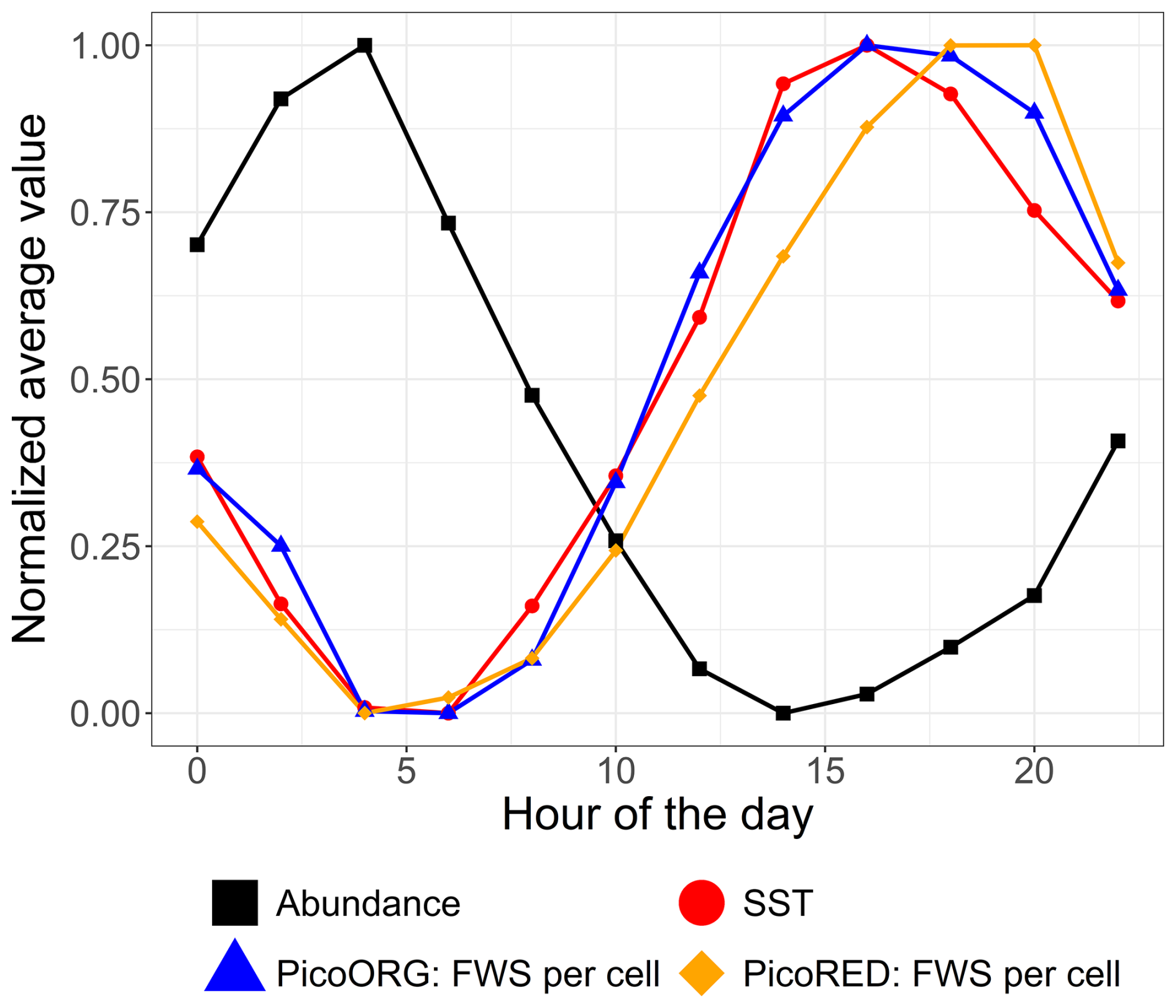
Figure 14 Mean average abundance, SST, and cell size proxy (FWS) of the PicoORG (Synechococcus spp. like) and PicoRED (picoeukaryote) groups normalized (between 0 and 1 using the following formula: $\frac{y-y_{\min }}{y_{\max }-y_{\min }}$) for each hour of the day for the 2022 data after 9 June.

SST plays a crucial role in driving picoeukaryotes and cyanobacterial dynamics, both periodically (e.g., daily cycles) and non-periodically (e.g., marine heat waves). This link is consistent with previous studies (Chen et al., 2014; Hunter-Cevera et al., 2020). As EEC coastal waters warm due to global change (+1 °C over the past 10 years, with a projection of $+\mathrm{3.34}\pm \mathrm{0.88}$ °C by 2100; Hubert et al., 2025a; Tinker et al., 2024), monitoring the long-term high-frequency dynamics of picophytoplankton, in addition to other size classes, is of the utmost importance. These organisms are critical to pelagic food webs and biogeochemical cycles (Xiu-ren and Vaulot, 1996), and understanding how they will respond to warming and the associated rare events is crucial.

5 Conclusions

This study characterizes the multiscale dynamics of phytoplankton during the springs of 2021 and 2022 off the Liane estuary and the Boulogne-sur-Mer coastal area in the eastern English Channel. We showed the seasonal successions between key phytoplankton functional groups (PFGs), particularly between the MicroRED (mostly diatoms) and NanoRED (mostly haptophytes of the genus Phaeocystis globosa) groups. Using empirical mode decomposition and the Lomb–Scargle periodogram method, we identified various modal fluctuations across different temporal scales in phytoplankton abundance, red fluorescence (a proxy of chlorophyll a), and the Shannon diversity index, highlighting the complex dynamics of population assemblages.

Our findings reveal that much of the variability in these time series occurs at short timescales, particularly on the order of a few hours. This indicates that low-frequency sampling may miss significant dynamics in phytoplankton communities. We also observed that these multiscale fluctuations do not stabilize over time, particularly during the seasonal shifts in community assemblage, such as the dominance of pico-organisms in the summer of 2022, when sea surface temperature became a major driver of abundance.

The study's limited duration, constrained by the system's design, suggests the need for longer-term monitoring of PFGs, coupled to high-frequency measurements of more abiotic variables such as nutrients, light, and mixing, in order to assess whether high-frequency fluctuations become less significant over larger temporal scales (e.g., interannual variations) in the context of global change and changing anthropogenic pressures. This gives better understanding of the mechanisms of their impact on the whole size range of the main marine primary producers. Additionally, incorporating higher trophic levels, such as zooplankton, could offer insights into top–down control mechanisms, which were not fully addressed here. As noted previously, seasonal variations – which are essential for understanding phytoplankton dynamics – were not fully captured in this study due to its limited temporal coverage. This highlights the need for future research based on longer monitoring periods.

Overall, this study confirms the interest and great potential of combining automated flow cytometry with fixed buoys for high-frequency monitoring of marine ecosystems, though the system's design requires adaptation for long-term use. Given the increasing frequency of rare events like storms, estuarine loads, and heat waves in coastal areas, automated monitoring, coupled with robust statistical analyses, is crucial for understanding phytoplankton variability and its impact on marine food webs and biogeochemical cycles. This approach can provide valuable data for models predicting changes in ecosystem structure and function.

Appendix A: Glossary

The definitions of the abbreviations used in this article are provided below.

Abbreviation	Definition
EEC	Eastern English Channel
EMD	Empirical mode decomposition
FLO	Orange fluorescence
FLR	Red fluorescence
FLY	Yellow fluorescence
FWS	Forward scatter
IMF	Intrinsic mode function
LSP	Lomb–Scargle periodogram
PFG	Phytoplankton functional group
ROFI	region of freshwater influence
SST	Sea surface temperature
SWS	Sideward scatter

Appendix B: Cross-covariance function of the 2022 FLR data

The cross-covariance functions between the water height data (REFMAR data; SHOM, 2024) and the FLR data before and after 9 June 2022 are displayed in Fig. B1. An inversion of the link between the two time series was observed, as was also the case between the water height and the abundance data (Fig 10). This link was still less important after 9 June, as the area was dominated by pico-organisms.

Figure B1 Cross-covariance functions between the water height data (REFMAR data; SHOM, 2024) and the FLR data before and after 9 June 2022.

Appendix C: Relative time series: stacked area representation

The relative abundances and FLR values for the two deployments are shown as stacked area plots in Fig. C1. The same patterns described previously are evident: spring shifts in the abundance time series (Fig. C1a) from picophytoplankton to nanophytoplankton and, in the FLR time series (Fig. C1b), from microphytoplankton to nanophytoplankton. The dominance of pico-organisms – particularly PicoORG – during summer is also observed in the 2022 data. Some rare events are noticeable as well, such as the relative increase in MicroRED during the strong-wind event of May 2021, visible as an expansion of the black area. Quick shifts, corresponding to high-frequency fluctuations, are also observable throughout the time series.

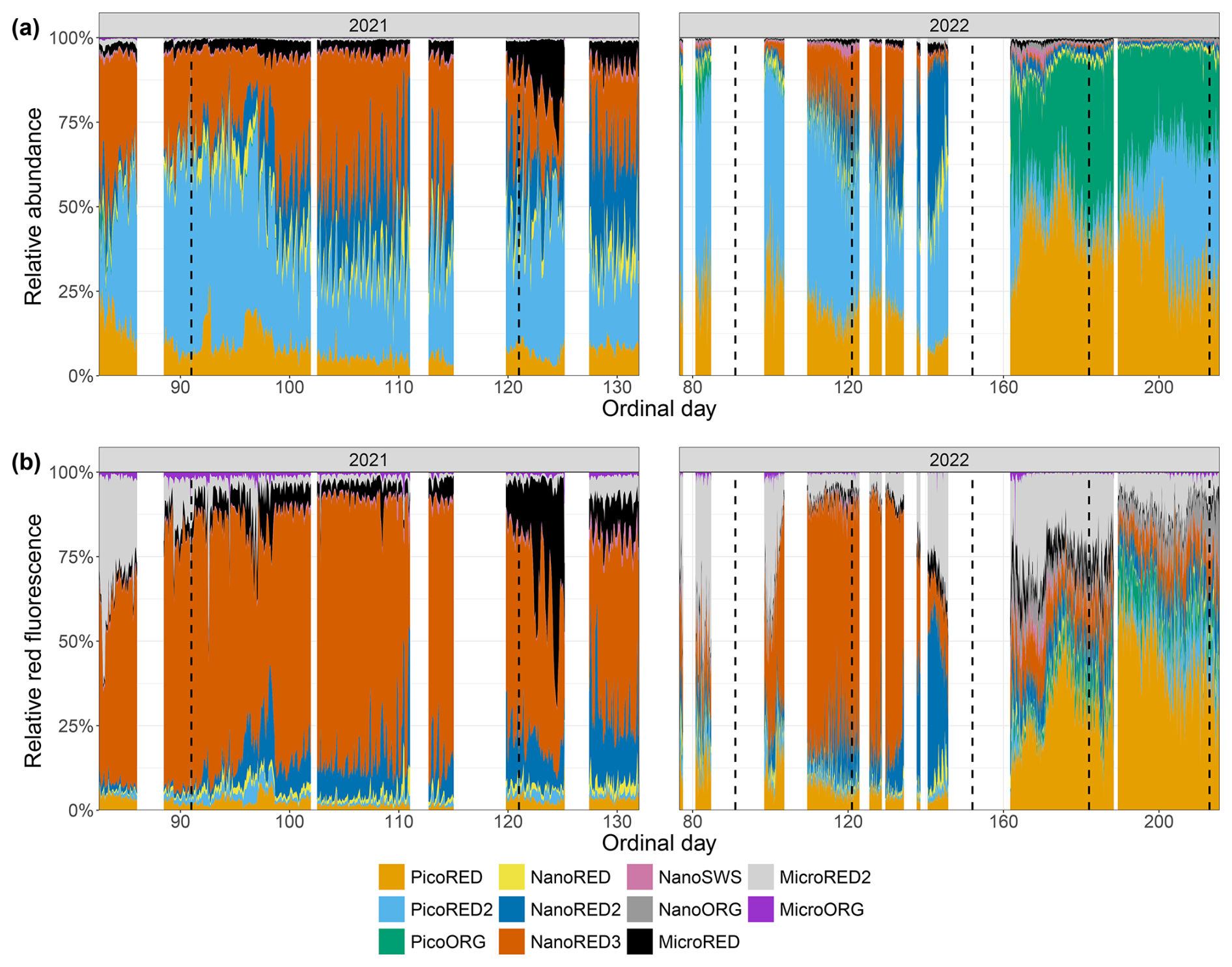
Figure C1 Phytoplankton data recorded for each group with the automated flow cytometer (CytoSub) for each sampled ordinal day: (a) PFG relative abundance and (b) PFG relative red fluorescence (proxy of chlorophyll a). The relative values of each group are computed as the ratio of the group's value to the total sum across all of the groups. The stacked colored areas represent the relative value for each PFG. The black dashed lines indicate the start of each month.

Appendix D: Wind directions during the rare events

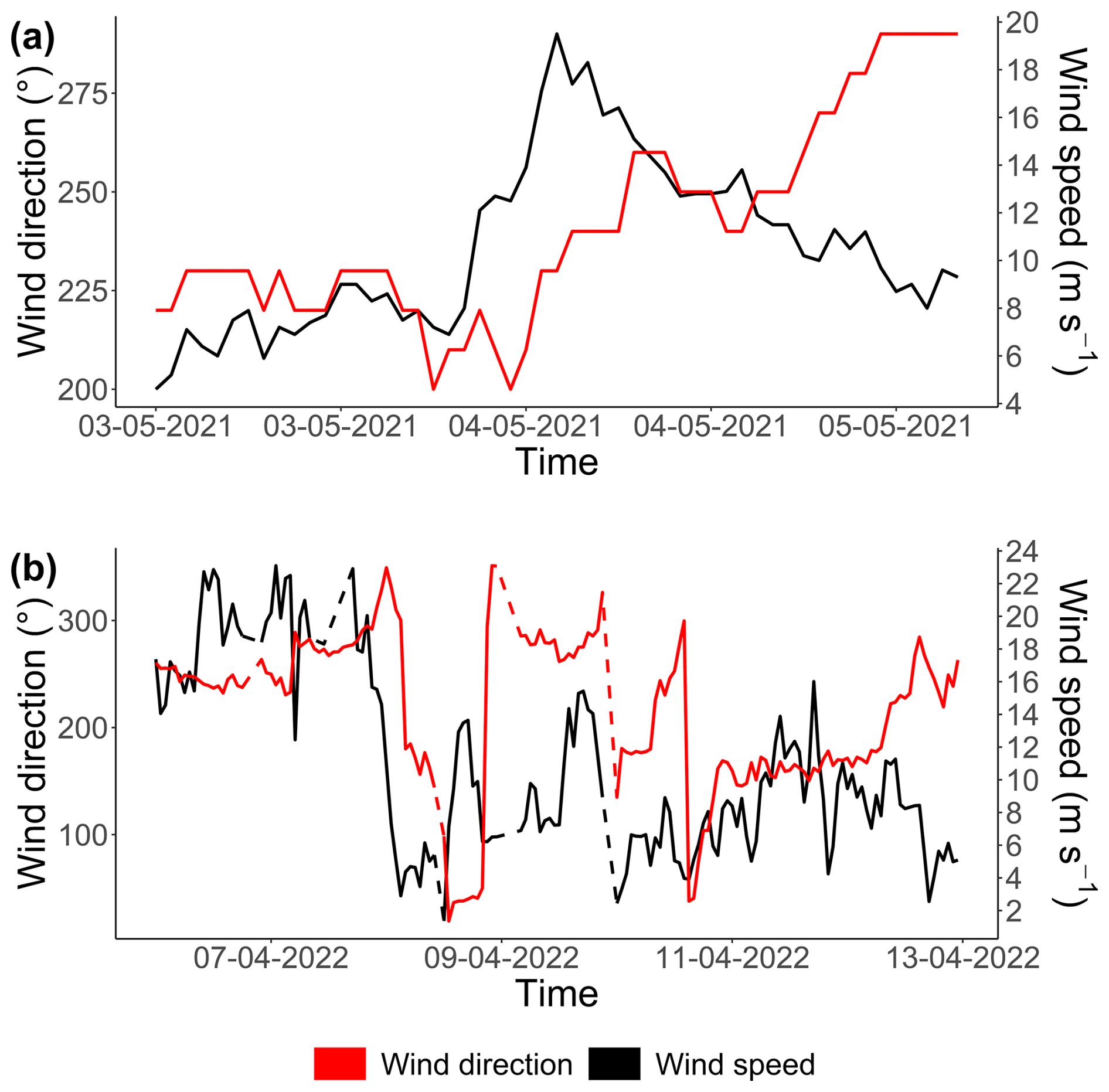
The wind directions observed during the two strong-wind events (see Fig. 7) are shown in Fig. D1. As mentioned previously, the 2021 event was characterized by strong southwesterly winds (ranging from 200 to 260°). In 2022, the event initially featured southwesterly winds (although PFG data were not available for this period), followed by northeasterly winds during the peak in abundance highlighted in Fig. 7. Unfortunately, wind data were not available precisely during this abundance peak.

Figure D1 Wind direction (red line, in degrees from true north) and wind speed (black line; m s⁻¹) recorded during the two strong-wind events shown in Fig. 7: (a) May 2021 and (b) April 2022. Dashed lines indicate gaps in the time series due to missing data.