Determining the depth and upwelling speed of the equatorial Ekman layer from surface drifter trajectories

In this work, trajectories of more than 500 drogued surface drifters launched in the equatorial ocean since 1979 are analyzed by employing the results of a new Lagrangian theory of poleward transport from the Equator forced by the prevailing trade winds. The Lagrangian theory provides an explicit expression for the depth of the Ekman layer that circumvents the application of the 3D continuity equation that requires calculation of the divergence of horizontal transport, which has been the basis of all previous studies on the subject. The analysis is carried out for drifters launched within 1° of the Equator that reached a final latitude of 3, 4, or 5° north or south of the Equator while also remaining in one hemisphere throughout their entire travel time. The analysis yields robust estimates of 45 m for the Ekman layer's depth and 1.0 m d⁻¹ for the upwelling speed of thermocline water into the layer.

1 Introduction

The trade winds, which blow westward in the tropics due to action of the Coriolis force on the northerly surface winds of the Hadley circulation, are the first and most basic component of the heat transport from the warm equatorial surface ocean to the cold poles that mitigates the overall pole-to-Equator temperature gradient on Earth. The mechanism that enables the poleward, temporally independent heat transport is the surface flow in the ocean that is directed 90° to the right or left of the wind in the respective Northern Hemisphere or Southern Hemisphere relative to the direction of the overlying wind. This counterintuitive flow direction results from Earth's rotation, which adds the Coriolis force to the stress applied by the winds at the ocean surface. This straightforward scenario of wind-driven ocean circulation appears in all textbooks (Knauss, 1996; Talley et al., 2011); however, despite its convincing simplicity, quantitative estimates of the parameters that control it currently vary widely depending on the data and method used in the calculations of these estimates.

The classical theory that describes the ocean response to forcing by the overlying winds was developed about 120 years ago by Ekman (1905) under the assumption of constant Coriolis frequency. This assumption greatly simplifies the analysis by ensuring that all coefficients in the governing equations are constant. The dynamics described in Ekman's theory includes a steady flow perpendicular to the wind direction and inertial, i.e., force-free, oscillations at the local (constant) Coriolis frequency. This is in sharp contrast to actual conditions in the equatorial region, where the Coriolis frequency vanishes at the Equator and varies (linearly) with latitude. The latitudinal variation in the Coriolis frequency turns the equations nonlinear and the oscillation-free flow unsteady, in contrast to Ekman's original midlatitude theory. The poleward-directed surface flows in both hemispheres along the Equator imply a strong horizontal divergence along the Equator that can only be balanced by the upwelling of deeper water into the wind-forced Ekman layer. Although the heuristic application of the midlatitude Ekman theory to the vicinity of the Equator is quite straightforward, it has not previously been able to be employed to estimate the depth of the equatorial Ekman layer or the rate of upwelled volume of water.

The complications that result from the inclusion of the meridional variation in the Coriolis frequency in Ekman's theory were recently resolved in a theory of wind-driven flow, in which the classical theory of Ekman (1905) was extended to the equatorial region (Paldor, 2024). This new theory employs the adiabaticity method (Goldstein, 1980; Paldor and Friedland, 2023) that filters out fast oscillatory dynamics from the slow dynamics associated with the motion of the center of oscillation. In the context of the equatorial Ekman problem, the eliminated oscillations result from the meridionally varying Coriolis force, while the slow and monotonic poleward motion results from the combination of the wind stress and the Coriolis force. The essence of the method is the formulation of the problem as the dynamics of a (quasi-)particle about the minimum of a potential, while the potential itself varies with time on a slower timescale than the period of oscillations about the minimum. The potential is derived from the meridional Lagrangian momentum equation when the zonal velocity, U, is expressed as follows: $U=D+\int f\left(y\right)\mathrm{d}y$, where f(y) is the latitude-dependent Coriolis frequency (=βy near the Equator) and D is the pseudo-angular momentum, the latter of which is conserved in the absence of other (body) forces. The substitution of the angular momentum for the zonal velocity is essential for the analysis in spherical coordinates (RomKedar et al., 1997). Additional details of the theory are given in Sect. 2.1.

Direct observations of the depth (thickness) of the equatorial Ekman layer and the rate of upwelling water to it are difficult to quantify due to the poor observational definition of the layer's dimensions and the extremely low speed of upwelling. Halpern and Freitag (1987) and Johnson et al. (2001) estimated the upwelling rate in the equatorial Pacific Ocean above 50 m depth to be about 2 m d⁻¹ based on the divergence of several moored horizontal current meters. Below 50 m depth, their estimated vertical velocity is negative (directed downward). A similar upwelling rate of 2 m d⁻¹ extending to depths of 120 m was estimated by Halpern et al. (1989) between 110 and 140° W from December 1983 to September 1984 (but excluding April 1984) using the same method of inferring vertical speeds from the divergence of horizontal currents measured by moored current meters. The upwelling speed decreased eastward in these observations, and the variation in the observed values greatly exceeded the mean values. In the same region (central Pacific) but in February–March 1980, Bubnov (1987) used a similar method of integrating the 3D continuity equation associated with observed horizontal currents and estimated the upwelling velocity over the upper 300 m to vary between 1 and 8 m d⁻¹.

Surface drifter trajectories deployed in the eastern Pacific during 1977–1982 were used by Hansen and Paul (1987) as proxies for the currents, while the trajectory divergence was used as a proxy for the current's divergence; this yielded an upwelling speed of 1.5 m d⁻¹ in a region spanning ±1.5° from the Equator. The idea underlying their analysis was that the drifter trajectories represent the currents and divergence in the top 50 m. As noted by the authors, the main issue with their analysis was the accuracy of the representation of currents by drifter trajectories. Using over 700 drifters launched between 1979 and 1990, Poulain (1993) estimated an upwelling velocity of 15–20 m d⁻¹ between 90 and 150° W in the equatorial Pacific. The method used by Poulain (1993) in the interpretation of drifter observations was to average the drifter velocities in given geographical domains and at selected time intervals to generate the Eulerian velocities at the center of the domain at that time. The high values of upwelling velocity in this study result from the small areas used for inverting the observed Lagrangian drifter velocities to Eulerian fields. Two important conclusions emerge from that study: (1) except for its western part, the horizontal divergence in the equatorial Pacific is quite uniform, meaning that the upwelling speed should also be quite uniform; (2) the upwelling velocity decreases monotonically with the assumed width of the meridional band over which the horizontal divergence is calculated.

Estimates of upwelling rates have also been calculated based on the distribution of ¹⁴C, which was released to the atmosphere in large amounts from aboveground nuclear tests between 1955 and 1963. An analysis of the oceanic uptake of ¹⁴C and its redistribution in the Pacific Ocean carried out by Quay et al. (1983) yielded a value of about 0.3 m d⁻¹ for the upwelling velocity along the Equator. Aside from this geo-isotopic study, previous estimations of the horizontal divergence fields have been obtained either directly from current meter observations or indirectly from drifter trajectories. In the latter case, those data were either spatially averaged to yield the Eulerian fields or interpreted as proxies for these fields. In contrast, the current study directly applies a recently developed Lagrangian dynamical theory to observed drifter trajectories, thereby bypassing the need to first estimate the horizontal divergence. The large number of drifters, the accurate tracking of their location by satellites, and the long period of temporal coverage allows for the selection of a sufficient number of drifter trajectories to satisfy predetermined selection criteria and yield accurate estimates of the depth of the equatorial Ekman layer and the speed of upwelling into it.

The remainder of this paper is structured as follows: the application of the Lagrangian theory to drifter observations and the data used in this study are detailed in Sect. 2; in Sect. 3, we give the results obtained by applying the theory to drifter trajectories; and the study is summarized in Sect. 4.

2 Theory and data

2.1 Theory

The recent extension of the wind-driven theory of ocean circulation to the Equator described in Paldor (2024) has demonstrated that, as in Ekman's original theory, the oceanic response can be decomposed into a monotonic, slow flow (which is directed poleward in the equatorial region) and fast, large-amplitude oscillations. In contrast to Ekman's original theory, when the wind stress is directed westward in the equatorial region, the oscillations are highly nonlinear and of large amplitude. An example of the large-amplitude inertial oscillations associated with an initial impulse of a westward-directed velocity when no wind stress affects the motion is shown in Fig. 1a. The present study applies the explicit expressions developed in Paldor (2024) to the observed trajectories of surface drifters by modifying the nondimensional variables and parameters in Eq. (10) of Paldor (2024). The dimensional counterpart of this equation

$$\begin{array}{}\text{(1)}& {\displaystyle \frac{\mathrm{d}y}{\mathrm{d}t}}={\displaystyle \frac{\mathrm{1}}{y\left(t\right)}}{\displaystyle \frac{-{\mathit{\tau }}^x}{H}}\left({\displaystyle \frac{R_{\mathrm{e}}}{\mathrm{2}\mathrm{\Omega }\mathit{\rho }}}\right).\end{array}$$

Here, y(t) is the distance from the Equator at time t. The global parameters in this relation are as follows: $\mathit{\rho }=\mathrm{1027}\mathrm{kg}{\mathrm{m}}^{-\mathrm{3}}$ (water density), $\mathrm{\Omega }=\mathrm{7.29}\times {\mathrm{10}}^{-\mathrm{5}}{\mathrm{s}}^{-\mathrm{1}}$ (Earth's rotation frequency), and $R_{\mathrm{e}}=\mathrm{6371}\times {\mathrm{10}}^{\mathrm{3}}\mathrm{m}$ (Earth's radius). Thus, $\left(\frac{R_{\mathrm{e}}}{\mathrm{2}\mathrm{\Omega }\mathit{\rho }}\right)=\mathrm{4.25}\times {\mathrm{10}}^{\mathrm{7}}{\mathrm{m}}^{\mathrm{4}}\mathrm{s}{\mathrm{kg}}^{-\mathrm{1}}$. The remaining specific parameters are as follows: τ^x, which represents the wind stress (in N m⁻²; negative for easterly winds), and H, which represents the Ekman layer's depth (in meters).

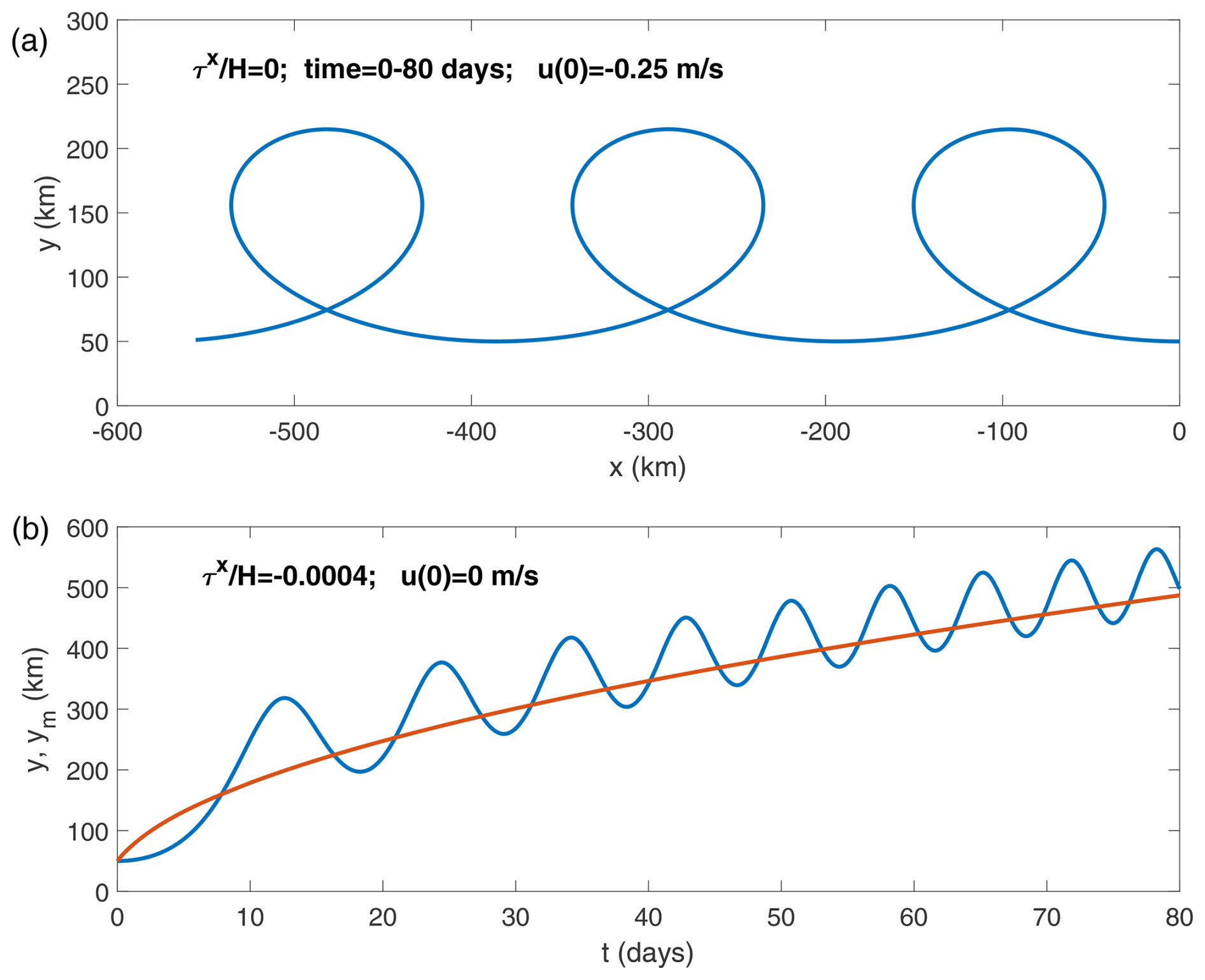
Figure 1 (a) The numerically calculated geographic trajectory of a water column initiated with a westward-directed impulse of 0.25 m s⁻¹ zonal velocity subject only to the (latitude-dependent) Coriolis force. (b) The latitude (i.e., distance from the Equator in kilometers) time series (blue curve) and the oscillation-free latitude time series given by Eq. (2), denoted here by y_m (red curve), of a 50 m thick water column forced by a westward-directed wind stress (τ^x) of 0.02 N m⁻². In both panels, the initial distance from the Equator is y(0) = 50 km, while the initial longitude and the initial meridional velocity are both 0.

Multiplying the nonlinear relation Eq. (1) by y(t) and integrating the resulting first-order equation for y(t)² yields

$$\begin{array}{}\text{(2)}& y{\left(t\right)}^{\mathrm{2}}=y{\left(\mathrm{0}\right)}^{\mathrm{2}}+\mathrm{2}{\displaystyle \frac{-{\mathit{\tau }}^x}{H}}\cdot \left({\displaystyle \frac{R_{\mathrm{e}}}{\mathrm{2}\mathrm{\Omega }\mathit{\rho }}}\right)t.\end{array}$$

As demonstrated in Fig. 1, this expression (shown by the red curve) successfully filters out the inertial oscillations from the actual latitude time series (blue curves) and describes the net, oscillation-free, poleward motion.

Inverting Eq. (2) to an explicit expression for H, setting t to t_i (the travel time of drifter #i) and y(t) to L (a “boundary” of the equatorial region) yields the estimate of H_i (the depth value based on trajectory #i):

$$\begin{array}{}\text{(3)}& H_i=\left({\displaystyle \frac{R_{\mathrm{e}}}{\mathrm{2}\mathrm{\Omega }\mathit{\rho }}}\right){\displaystyle \frac{\mathrm{2}\left(-{\mathit{\tau }}^x\right)}{L^{\mathrm{2}}-y_i{\left(\mathrm{0}\right)}^{\mathrm{2}}}}{t}_i,\end{array}$$

where y_i(0) is the distance of drifter #i from the Equator at t=0 (i.e., the distance of the launch point from the Equator).

2.2 Drifter trajectories

Nearly 30 000 surface drifters have been released at the ocean surface since 1979 (Lumpkin et al., 2017), and the geographical trajectories of these drifters have been tracked by satellites every 6 h for periods of up to 1000 d. These (Lagrangian) observations cover the global ocean, and a few percent of these drifters were launched on both sides of the Equator in the Pacific, Atlantic, and Indian oceans. The slightly negatively buoyant drifter is typically drogued at a 15 m depth, so it provides an estimate of the current in the top 15 m of the water column, where the wind stress is the primary forcing (Lumpkin et al., 2017). The agreement between drifter trajectories and ocean currents demonstrated in Lagerloef et al. (1999) and assumed in Poulain (1993) motivates an analysis of observed drifter trajectories in order to determine the depth of the equatorial Ekman layer and the upwelling speed of deep water into it.

The drifter trajectories used in the analysis are freely available from the NOAA Global Drifter Program (NOAA/AOML/GDP) site. The data were screened according to the following three criteria:

1. The drifters were launched within 1°≈110 km south or north of the Equator (regarded as the Equator).

2. Once launched, the drifters remained in one hemisphere throughout the entire travel time to their final latitude (this is because crossing the Equator is not possible under the assumed westward-directed wind stress).

3. The drifters were continuously tracked, with gaps no longer than 1 d, during their motion from their launch point to their final latitude that marks the boundary of the equatorial region (i.e., 3°≈330 km, 4°≈440 km, or 5°≈550 km).

The latitudes 3 and 4° have been used in previous studies to define the boundaries of the equatorial region (Brady and Bryden, 1987; Lagerloef et al., 1999; Johnson et al., 2001); however, in the present study, we also used $L=\mathrm{5}\mathit{°}\approx \mathrm{550}\mathrm{km}$ to verify the robustness of the calculated averages to the selected values of L. The case L=2° is not included in the analysis because the singularity of Eq. (3) at L²=y_i(0)² affects the accuracy of the estimates of H_i when L is close to y_i(0); i.e., for $L=\mathrm{2}\mathit{°}\approx \mathrm{220}\mathrm{km}$ and for y_i(0)≤1°, the denominator is tiny, which can yield an extremely high value of H_i and amplify observational errors.

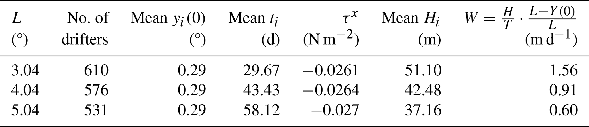
As of August 2024, ∼ 30 000 drifter trajectories have been archived in the Atlantic Oceanographic and Meteorological Laboratory (AOML) archive, and over 1500 drifters have been launched near the Equator and reached final latitudes of 3,4, or 5°, of which ∼ 700 drifters remained in one hemisphere. The number of drifters in the Atlantic and Pacific oceans that reached each of the final latitudes is given in the second column of Table 1; Table 1 also gives the mean y_i(0) (≡Y(0), third column) and the mean travel time t_i, (≡T, fourth column) to the final latitudes (noted in the rows of this table). The Indian Ocean is excluded from the analysis due to the positive mean annual wind stress over the waterbody (see Sect. 2.3). No screening was made of drifters that lost their drogues on their way from y_i(0) to L.

2.3 Wind stress

The daily wind stress values over the oceans (τ^x) used in this work are available at the NOAA/CoastWatch site at a 0.125° spatial resolution for the 1999–2009 period. We calculated the averaged wind stress for the whole period in the entire region of the Indian, Atlantic, and Pacific oceans in a zonal strip that straddles the Equator between −L and +L, where L corresponds to 3, 4, or 5°.

These wind stress averages are given in the fifth column of Table 1 for the Atlantic and Pacific oceans (where the mean stresses in the two oceans differ by no more than a few percentage points) but not for the Indian ocean, where the calculated mean values of the wind stress are positive (so H_i<0) and small (less than $+\mathrm{0.01}\mathrm{N}{\mathrm{m}}^{-\mathrm{2}})$, probably due to the strong seasonal forcing by the monsoon system that induces eastward-directed zonal winds during part of the year over this ocean (Hastenrath and Polzin, 2004; Zhang et al., 2022). The decade-long zonal wind stress observations are considered representative of the climatic values that prevailed throughout the trajectories of all drifters. Although the negative mean temporal values of τ^x in the Atlantic and Pacific oceans are not spatially uniform (reaching their maximal values in the center of each ocean and tapering off near the continents that bound the ocean on the eastern and western sides), only the spatial mean values are used.

Table 1 Drifter characteristics in the Pacific and Atlantic oceans and the zonal wind stresses over these waterbodies. The shown values of L are larger by a few kilometers compared to the distances corresponding to 3,4, or 5°, as a drifter is determined to be “at L” with an offset of up to 6 h after its passage of that point. Less than 10 % percent of the relevant drifters were launched in the Indian Ocean, which is not included in this table or in the analysis because the annual mean wind stress over this waterbody is directed eastward, inconsistent with a poleward-directed net motion. The fifth column denotes the daily mean wind stress values over the entire 1999–2009 period in each ocean used in this study. The variables H, T, and Y(0) denote the mean values (over all drifters) of H_i, t_i, and y_i(0), respectively.

3 Results

Four representative drifter trajectories are shown in Fig. 2, and they demonstrate the richness of observed trajectories near the Equator, the intricate combination of oscillations with slow poleward propagation, and the occurrence of equatorial crossings for many trajectories.

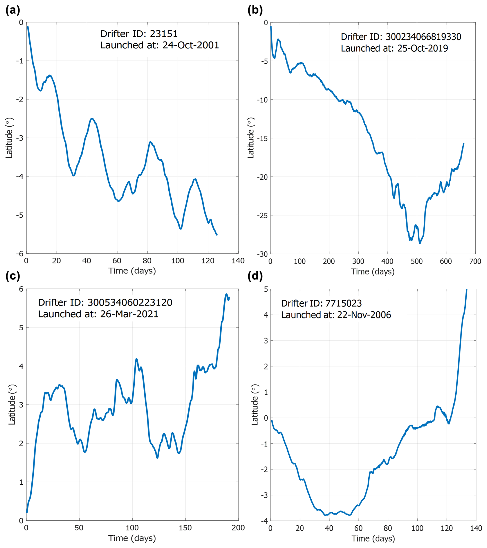
Figure 2 Four drifter trajectories originating within 1° of the Equator that were analyzed in this study: (a) a typical Southern Hemisphere trajectory that clearly shows oscillations and a mean poleward flow; (b) a fast Southern Hemisphere trajectory that reaches 4° in just a few days and remains operational for nearly 2 years; (c) a slow Northern Hemisphere trajectory that reaches 4° in more than 100 d; (d) part of a trajectory that reaches 3° prior to crossing the Equator. The trajectory in panel (d) is included in the analysis of L=3° but not in the L=4° or L=5° analyses, as it only reaches L=4° or L=5° after crossing the Equator.

Substituting the values of y_i(0) and t_i for each drifter into Eq. (3) yields the corresponding values of H_i. The sixth column of Table 1 gives H, the mean of the particular values of H_i, while the histograms of the H_i values for each value of L are shown in Fig. 3; thus, the value of H is best estimated by $H=\mathrm{44}\pm \mathrm{7}\approx \mathrm{45}$ m.

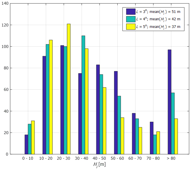
Figure 3 Histograms of the H_i values for the three values of L. For L=3°, the tail of H_i>80 m is as high as the maximum cell of H_i= 20–30 m, consistent with the singularity of Eq. (3) at L=y_i(0).

Equation (2) can also be employed to calculate the poleward, oscillation-free velocity of a drifter on its way from y_i(0) to L=y(t_i) from the drifter's average speed during its travel: $V_i=\frac{L-y_i\left(\mathrm{0}\right)}{t_i}$. Thus, the volume divergence (per unit length in x) that results from the anti-parallel, poleward-directed volume fluxes of two water columns that are initially conjoined along the Equator and move poleward is $\mathrm{2}{H}_i{V}_i=\mathrm{2}{H}_i\frac{L-y_i\left(\mathrm{0}\right)}{t_i}$. The vertical volume flux (per unit length) due to Ekman upwelling during t_i is 2LW_i, where W_i is the upwelling speed. Equating the vertical and horizontal fluxes yields $W_{i}L=H_i\frac{L-y_i\left(\mathrm{0}\right)}{t_i}$ or $W_i=\frac{H_i}{t_i}\frac{L-y_i\left(\mathrm{0}\right)}{L}$. The mean values of H_i and t_i in Table 1, denoted by H and T, then yield the mean values of W (in the last column) that average to W≈1.0 m d⁻¹ for the three values of L.

The estimated H and W values along the equatorial Atlantic and Pacific oceans are noted in Fig. 4 using a qualitative sketch of the wind forcing and resulting oceanic flow patterns.

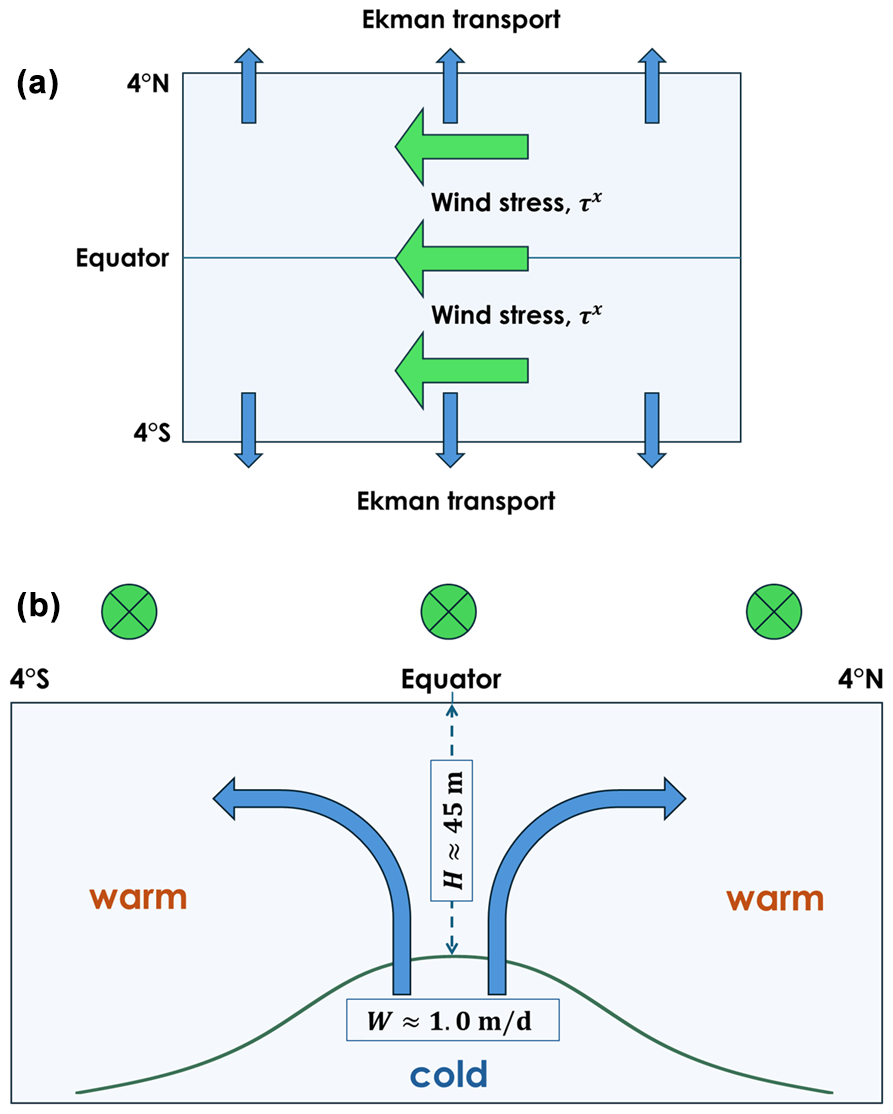
Figure 4 A sketch showing the poleward-directed, wind-driven surface flow along the Equator under westward-directed wind stress (planar view in panel a) which is compensated for by the upwelling of water from below (latitude–height cross-section viewed from the east in panel b). The dark-green curve in the lower panel denotes the boundary between the warm surface water and cold thermocline water. The H≈45 m and W≈1.0 m d⁻¹ estimates are the main results of this study.

4 Summary and discussion

The mean estimates of H=45 m and W=1  m d⁻¹ calculated here based on surface drifter trajectories are more robust compared to prior estimates derived from standard hydrographic observations. Table 1 shows that the present estimates of H vary with L by a few meters, whereas those for W vary by about 0.5 m d⁻¹. These variations are smaller than those of estimates based on standard hydrographic data that can vary by about 1 order of magnitude (Wyrtki, 1981; Brady and Bryden, 1987; Lukas and Lindstrom, 1991; Weingartner and Weisberg, 1991). As an example, the H=45 m value reported here exceeds the estimate of 30–40 m proposed in Lukas and Lindstrom (1991), but the O(10 %) variation in the present estimate is significantly smaller than the O(80 %) variation in the previous estimate. In view of the crucial role played by the poleward flow of warm equatorial water in mitigating the large, radiative pole-to-Equator temperature gradient (Czaja and Marshal, 2006; Hartmann, 2016), a reliable quantification of the initiation of this flow is important for understanding Earth's climate.

The zonal stress is not uniform, reaching a maximal value in the center of the ocean and tapering off towards the boundaries in the east and west. The effect of this variation on the value of H is pronounced in the equatorial Pacific Ocean, and calculations of H using the values of τ^x at each drifter's initial location yield a wider range of H values. These estimates are also not exact, as the value of τ^x varies with time and along the drifter trajectory. A detailed analysis of the variation in τ^x along a drifter trajectory and its effect on the value of H_i calculated in that trajectory are left for future work.

In contrast to Ekman's theory for the midlatitudes, the extension of this theory to the equatorial region implies that the slow, net poleward motion of a water column subject to zonal wind stress is accompanied by a zonal component. This results naturally from the inertial oscillations that involve net zonal translation on the Equator (as in Fig. 1a), while inertial oscillations on the midlatitude f plane are not accompanied by a translatory motion.

The results calculated in Sect. 3 focus on the net poleward propagation rate, which neglects the inertial oscillations, while the observed trajectories include both types of motion. The neglect of inertial oscillations in the observed trajectories is justified based on the fact that the period of these oscillations is much shorter than the temporal length of the averaged trajectory used for calculating H_i in Eq. (3). The high variability in the geographical trajectories, which is exemplified in Fig. 2, does not permit an estimate of the oscillations' period directly from the trajectories. However, for the values of ${\mathit{\tau }}^x=\mathrm{0.026}\mathrm{N}{\mathrm{m}}^{-\mathrm{2}}$ and H=45 m, the period of inertial oscillations can be estimated from the scale $P={\left(\mathit{\beta }\cdot \frac{{\mathit{\tau }}^x}{\mathit{\rho }H}\right)}^{-\frac{\mathrm{1}}{\mathrm{3}}}\approx \mathrm{5}$ d, which is much shorter than the typical 30–60 d trajectory length (see the mean t_i values in Table 1). Thus, during the relatively long drifter travel time, the poleward motion due to the oscillations averages out to zero, leaving the poleward motion of the oscillations' centers as the sole contributor to the net motion.

The results shown in Table 1 imply a decrease in the value H (and hence the value of W) with an increase in L. This result is not trivial because Eq. (3) is also satisfied with constant H_i provided that L²∝t_i for y_i(0)≪L. However, the calculated mean t_i values for different values of L reported in Table 1 only show a power slightly above 1.0 but significantly smaller than 2.0. The variation in H with L probably originates from a mechanism similar to that depicted by the blue arrows in Fig. 4b, where the depth of the Ekman layer becomes shallower with distance from the Equator, affecting the relation between T and L. The suggested mechanism is reminiscent of the thinning of smoke billows far from the smoke stack, but we note that the transition from Eq. (1) to Eq. (2) is valid only when H is independent of t and y.

Although no explanation is proposed here for the quantitative dependence of H on L, this result is consistent with the results reported in Fig. 3 of Poulain (1993), who showed that the horizontal divergence decreases monotonically with the width of the latitudinal band. We also note that Eulerian calculations of $\frac{\partial v}{\partial y}$ based on spatial averaging of the Lagrangian observations, as was done in Poulain (1993), yield an estimate of $W/H$; therefore, additional information is needed for determining each of these parameters (Poulain, 1993, arbitrarily assumed H=50 m). In contrast, in the present study, H is determined directly from drifter trajectories, which yields an estimate of W based on mass conservation in a box of meridional extent 2L, thickness H, and unit zonal length.

The successful application of the new dynamical theory of wind-driven equatorial transport in the ocean developed in Paldor (2024) lends credence to the relevance of this theory to observations in the equatorial ocean and, in particular, to the use of the velocity at 15 m as representative of the surface Ekman layer. This relevance is demonstrated despite the omission of important factors such as the meridional wind stress (can be significant at short timescales), the initial drifter velocity (assumed to vanish in the theory), or the spatial and temporal changes in the zonal wind stress. It can be argued that the calculation and successful application of the oscillation-free speed of poleward wind-driven motion for the Equator is as significant to ocean dynamics as the development of the expression for the steady transport in the original f-plane Ekman theory.