Critical uncoupling between biogeochemical stocks and rates in Ross Sea springtime production–export dynamics

Three biogeochemical glider surveys in the Ross Sea between 2010 and 2023 were combined and analysed to assess production–export stock and rate dynamics. As the most productive of any Antarctic continental shelf, the Ross Sea is a site of substantial physical and biogeochemical interest. While this region and its annual bloom have been characterised for decades, logistical constraints, such as ship time and sea ice cover, have prevented a comprehensive understanding of this region over long (> 1–2 months) timescales and at high spatiotemporal resolution. Here, we use high-resolution datasets from autonomous gliders in mass balance equations to calculate short-term (days to weeks) net community production via oxygen concentration, change in particulate organic carbon (POC) concentration over time, and POC export potential during the period of peak primary production in the region (November–February). Our results show an overall decoupling of net community production (NCP), driven by biologic changes in oxygen, from overall biomass concentration as well as changes in POC over time. NCP and carbon change vary between seasons and appear related to changes in ice concentration and stratification. Substantial spatiotemporal variability exists in all datasets, but high-resolution sampling reveals short-term variations that are likely masked in other studies. Our study reinforces the need for high-resolution sampling and supports previous classifications of the Ross Sea as a high-productivity (average NCP range −0.7 to 0.2 g C m⁻² d⁻¹), low-export (average changes in POC over time range −0.1 to 0.1 g C m⁻² d⁻¹) system during the productive austral spring and sheds additional light on the mechanisms controlling these processes.

1 Introduction

The balance between organic carbon production and organic carbon export from the surface ocean has been intensely investigated in recent years because of the key role it plays in regulating global climate (Siegel et al., 2016; Henson et al., 2024). While long-term monitoring programmes have allowed certain oceanic regions to be well characterised (Karl and Church, 2014; Steinberg et al., 2001; Hartman et al., 2021), uncertainties surrounding these processes in certain regions, such as the Southern Ocean, have limited our global understanding of this balance. However, the proliferation of autonomous assets, such as autonomous underwater vehicles (AUVs), profiling floats, and gliders, equipped with biogeochemical sensors, have allowed more and new measurements of carbon production and export processes at very high spatial and temporal resolutions, in places where sampling is challenging (Kaufman et al., 2014; Alkire et al., 2014). Despite these substantial advances in recent years, some regions still lack a long history of high-resolution observations, making it difficult to differentiate between general trends or anomalous events in a system.

One of these regions is the Ross Sea, which is a key region for organic and inorganic carbon cycling but continues to lack a complete, long-term understanding of biogeochemical dynamics because of logistical constraints. Shipboard and modelled estimates of primary production (Smith et al., 2000, 2013; Schine et al., 2015), carbon concentrations (Sweeney et al., 2000), and carbon export (Nelson et al., 1996; Collier et al., 2000) have been conducted in the Ross Sea since the 1970s but have been limited to discrete sampling in select locations. Moreover, substantial cloudiness in the region limits ocean colour satellite retrievals in the Ross Sea. Satellite bio-optical algorithms are derived primarily from low-latitude and mid-latitude biogeochemical properties (Hu et al., 2019), making satellite biogeochemical measurements from the Ross Sea both difficult and frequently inaccurate because of the substantial differences between these properties in high-latitude versus low-latitude regions (Chen et al., 2021).

Despite these limitations, the importance of the Ross Sea in Southern Ocean carbon cycling is clear. The Southern Ocean as a whole plays a disproportionately important role in global carbon dynamics, accounting for 40 % of carbon uptake (DeVries, 2014), and the Ross Sea is responsible for 28 % of that, despite only accounting for approximately 10 % of the global ocean surface (Arrigo et al., 2008). An important metric for evaluating the relationship between primary production and carbon export is the total amount of carbon that is converted to biomass after losses associated with autotrophic and heterotrophic respiration have been accounted for; this is termed net community production (NCP). Under steady-state conditions (i.e. carbon accumulation and loss terms are balanced over long timescales), NCP can be related to carbon export and is thus an important metric in evaluating production–export dynamics in oceanic systems (Cassar et al., 2015).

The Ross Sea is characterised by pronounced seasonal cycles dominated by a productive spring to summer season alternating with a comparatively unproductive autumn to winter season driven by heterotrophic processes. The productive period is dominated by a well-described, large and sustained phytoplankton bloom dominated by two key groups: colonial and solitary forms of the haptophytes Phaeocystis antarctica and diatoms (Smith et al., 2014). This bloom has been shown to reach substantial concentrations of biomass with chlorophyll concentrations reaching anywhere from 6 to > 40 µg L⁻¹ (Smith et al., 2000, 2011; Portela et al., 2025). Additionally, the region supports a substantial number of higher trophic level organisms, including Adélie and emperor penguins; orcas; Weddell, crabeater, and leopard seals; and pelagic birds (Smith et al., 2014).

The Ross Sea consistently exhibits high rates of primary production (Arrigo et al., 2008; Smith et al., 2014), but the ultimate fate of that biogenic carbon remains uncertain (Lo Monaco et al., 2005; Gruber et al., 2019). Along with the North Atlantic (Frigstad et al., 2015; Hartman et al., 2010) and upwelling regions (Demarcq, 2009), widespread phytoplankton blooms make the Southern Ocean continental shelf, during the bloom period, one of the most productive regions on the planet (Smith and Kaufman, 2018; Buesseler et al., 2020). Despite this, some studies have found reduced carbon transfer efficiencies relative to other regions on seasonal and annual timescales (e.g. Southern Ocean flux transfer efficiencies ranging from 0.2 to 0.8; Buesseler et al., 2020). These findings are supported by modelling studies, thus leading to the classification of the Ross Sea as a high-production, low-export system (Henson et al., 2019).

We assess high-resolution carbon production and export dynamics in the Ross Sea from three independent glider deployments during the austral spring/summer in 2010–2011, 2012–2013, and 2022–2023 and calculate biogeochemical rates, including NCP, changes in particulate organic carbon (POC) over time ($\frac{\partial \mathrm{POC}}{\partial t}$), and carbon export potential (${\mathrm{export}}_{\mathrm{POC}}^{\ast }$). We also evaluate POC : chlorophyll ratios (C : Chl) to assess how production–export dynamics have changed through time and how differences between deployments relate to taxonomic controls on production and export. The measurements evaluated come from glider-based dissolved oxygen, optical backscatter, and fluorescence data, with the latter two converted to POC and chlorophyll concentrations, respectively. This study is the first to use consistent methodology to compare high-resolution estimates of carbon production and export processes from different years on the Ross Sea continental shelf, providing further understanding of the role the Ross Sea plays in Southern Ocean carbon dynamics.

2 Methods

2.1 Glider deployments

Three deployments of autonomous Seagliders (Eriksen et al., 2001) equipped with biogeochemical sensors were completed in summer 2010–2011, 2012–2013, and 2022–2023 in the southwestern Ross Sea (Figs. 1, 2). Observational periods coincided with the onset and the majority of the annual spring phytoplankton bloom with gliders surveying from 22 November to 20 January (2010–2011; Kaufman et al., 2014; Queste et al., 2015), 31 November to 6 February (2012–2013; Jones and Smith, 2017; Meyer et al., 2022a), and 1 December to 19 January (2022–2023; Portela et al., 2025). All gliders were deployed from the fast ice near Ross Island (where calibration casts were not feasible) and recovered from the RVIB Nathaniel B. Palmer. For all three deployments, 93 %–95 % of all dives occurred within a 1° latitude by 1° longitude box of each mean survey location. Gliders were equipped with a Seabird CT sail (accuracy within 3.01 × 10⁻⁴ S m⁻¹, 0.001 °C, and 0.015 % for conductivity, temperature, and pressure, respectively; https://seabird.com, last access: 15 April 2025), an Aanderaa 4330F oxygen optode (accuracy of ∼ 1.5 %; https://aanderaa.com, last access: 15 April 2025), and a WetLabs ECO Triplet Puck (0.2 %–03 %; Salaun and Le Menn, 2023). Sensitivities for conductivity, temperature, pressure, oxygen, backscatter, and fluorescence were 4.0 × 10⁻⁵ S m⁻¹, 2.0 × 10⁻⁴ °C, 0.001 %, 3.2 µg L⁻¹, and 0.28 ppb per count, and 0.025 µg L⁻¹, respectively (https://seabird.com, https://aanderaa.com).

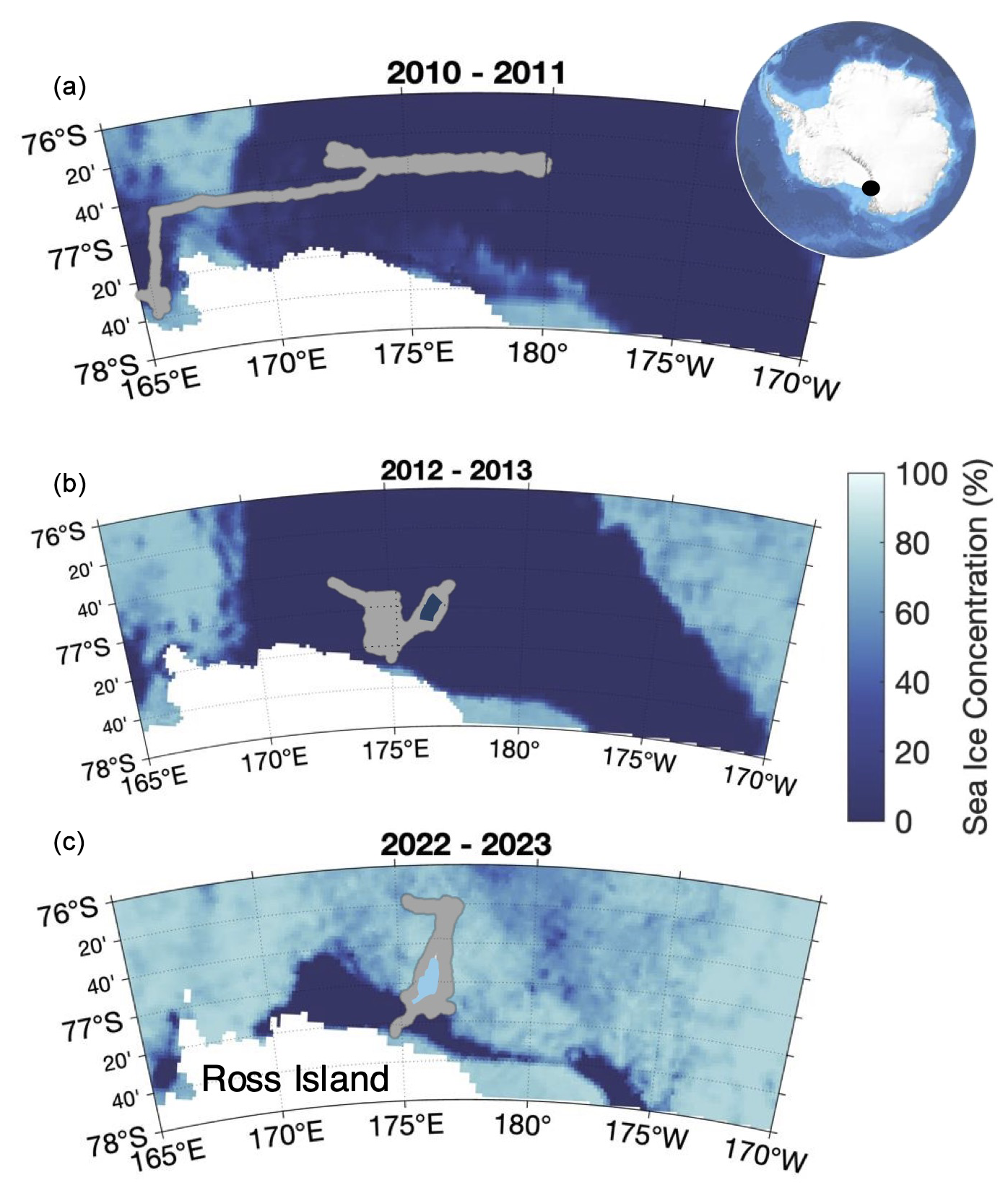
Figure 1 Maps of glider tracks from the 2010–2011 (a), 2012–2013 (b), and 2022–2023 (c) deployments overlaid onto average sea ice concentrations from 1 December of each year. Sea ice data come from the University of Bremen, and the inset map of Antarctica comes from Bedmap2. The white region indicates land, and the black dot indicates the location of Ross Island.

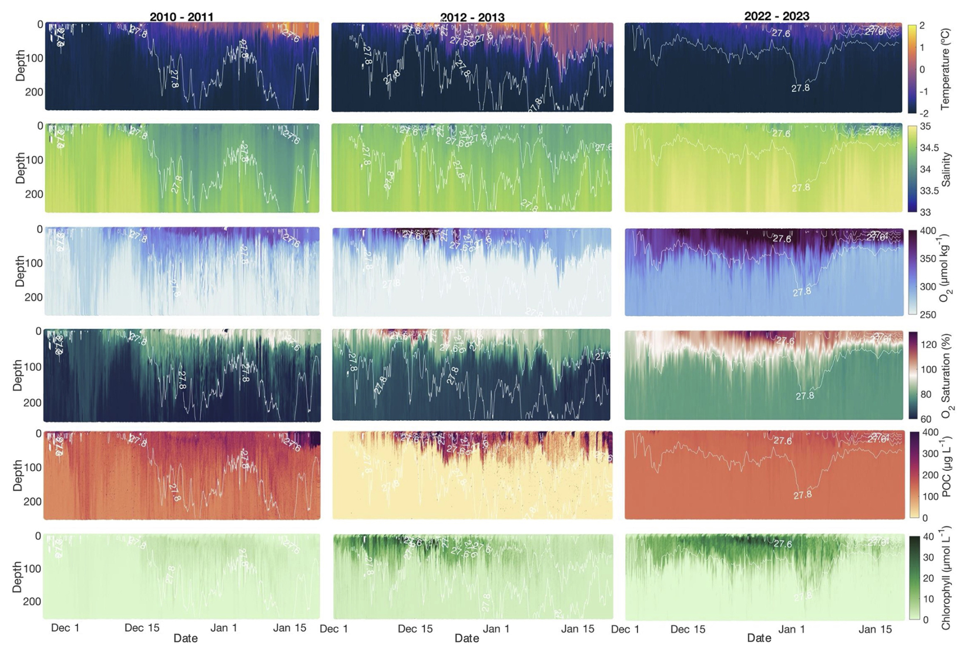
Figure 2 The 2010–2011, 2012–2013, and 2022–2023 glider profiles of temperature (°C), salinity, dissolved oxygen (µmol kg⁻¹), particulate organic carbon (POC) concentrations (µg C L⁻¹), and chlorophyll (µg L⁻¹) by date. Contours represent isopycnals. All profiles are for the upper 250 m.

CTD calibration casts were conducted by scientists aboard the RVIB Palmer in the near vicinity (< 400 m from the glider's location) coincident with glider recovery. Discrete samples were collected for chlorophyll a and POC. Chlorophyll a samples were analysed fluorometrically on the ship, whereas POC samples were stored and analysed onshore via an elemental analyser at the Virginia Institute of Marine Science (Gardner et al., 2000). Discrete chlorophyll a samples were used to convert glider fluorometer voltages to optically based chlorophyll, and discrete POC samples were used to convert optical backscatter counts at 470 nm wavelength ($b_{b_{\mathrm{p}}}\left(\mathrm{470}\right)$) to POC according to the method of Boss and Pegau (2001). For both chlorophyll and POC samples, single equations converting fluorescence to chlorophyll and backscatter to POC were individually generated per year (Fig. S1 in the Supplement). Dissolved oxygen sensors were factory calibrated and compared with profiles collected from the CTD rosette (R²=0.89, 0.76, and 0.96 for 2010–2011, 2012–2013, and 2022–2023, respectively). A full discussion of sensors, discrete samples, and calibrations is provided by Kaufman et al. (2014), Queste et al. (2015), Meyer et al. (2022a), and Portela et al. (2025).

2.2 Biogeochemical rate measurements

Three biogeochemical rates were calculated per deployment: NCP, $\frac{\partial \mathrm{POC}}{\partial t}$, and ${\mathrm{export}}_{\mathrm{POC}}^{\ast }$. Rates were calculated for non-overlapping, consecutive 3 d intervals over the duration of each deployment. To make the time period of analysis comparable between deployments, they were trimmed to only include days where euphotic zone (Z_eu)-averaged chlorophyll concentrations were within 90 % of the peak chlorophyll concentration (Fig. S2). Z_eu was calculated as 1 % of maximum measured photosynthetic active radiation (PAR) when PAR was available (2022–2023) or according to Morel (1974) when PAR was unavailable (2010–2011, 2012–2013). NCP was calculated via a mass balance of glider-based dissolved oxygen concentrations via Eq. (1):

$$\begin{array}{}\text{(1)}& {\mathrm{NCP}}_{\mathrm{100}}=\mathrm{PQ}\cdot \left(\underset{\mathrm{0}}{\overset{\mathrm{100}}{\int }}{\displaystyle \frac{\partial {\mathrm{O}}_{\mathrm{2}}}{\partial t}}-F_{K_z}-F_{\mathrm{Adv}}-{\mathrm{ASE}}_{\mathrm{ML}}\right),\end{array}$$

where PQ is photosynthetic quotient (i.e. the molar ratio of oxygen to carbon produced during photosynthesis), and ${\int }_{\mathrm{0}}^{\mathrm{100}}\frac{\partial {\mathrm{O}}_{\mathrm{2}}}{\partial t}$ is the change in O₂ concentrations integrated over the top 100 m from the beginning of day 1 to the end of day 3 of each 3 d period. A common reference depth is 100 m to assess carbon export efficiency, and thus it was chosen as our depth threshold (Buesseler et al., 2020). $F_{K_z}$ is the vertical eddy diffusion flux of oxygen to the water below 100 m, using the previously published vertical diffusivity coefficient (K_z) of 10⁻³ m² s⁻¹ for the Ross Sea (Kaufman et al., 2017). F_Adv is the advective flux of oxygen in the zonal and meridional directions with velocity calculated according to dive average currents (DACs) obtained from fitting a hydrodynamic model to the glider's flight path (Frajka-Williams et al., 2011). Because our glider surveys were not grids and thus limited our ability to generate individual x–y gradients, deployment-wide average DACs and zonal and meridional gradients of oxygen were used to calculate 3 d advection rates (F_Adv) for each 3 m depth bin (Fig. S3). Individual F_Adv values for each 3 m bin were then depth-integrated over 100 m to derive a value for each deployment according to Eq. (2):

$$\begin{array}{}\text{(2)}& F_{\mathrm{ADV}}=\underset{\mathrm{0}}{\overset{\mathrm{100}}{\int }}\left(u\cdot {\displaystyle \frac{\partial {\mathrm{O}}_{\mathrm{2}}}{\partial x}}+v\cdot {\displaystyle \frac{\partial {\mathrm{O}}_{\mathrm{2}}}{\partial y}}\right),\end{array}$$

where ASE_ML is air–sea exchange of oxygen between the atmosphere and the surface mixed layer. Mixed-layer depths were calculated according to potential density difference threshold of 0.02 kg m⁻³ from potential densities at 10 m. Air–sea exchange was calculated according to the bubble injection method outlined by Liang et al. (2013). Daily wind speed (m s⁻¹) and sea surface pressure (pascals) data come from the National Center for Environmental Prediction (NCEP) Reanalysis 1 product (2.5° × 2.5° resolution; Kalnay et al., 1996; Fig. 3e, g), which has been shown to be more accurate than ECMWF Reanalysis data in this region (Sanz Rodrigo et al., 2012; Fig. S4). The gas transfer velocity coefficient from Wanninkhof (2014) and the polar-specific photosynthetic quotient (1.3) from Laws (1991) were used. During the bloom period, we assume entrainment flux, lateral mixing, and vertical advection at the 100 m boundary to all be minimal; thus they are omitted. NCP data are presented in units of g C m⁻² d⁻¹ with positive values indicating net autotrophy (photosynthesis outpacing respiration) and negative values indicating net heterotrophy (respiration outpacing photosynthesis).

$\frac{\partial \mathrm{POC}}{\partial t}$ was calculated according to Eq. (3):

$$\begin{array}{}\text{(3)}& {\displaystyle }{\displaystyle \frac{\partial \mathrm{POC}}{\partial t}}=\underset{\mathrm{0}}{\overset{Z}{\int }}{\displaystyle \frac{\partial \mathrm{POC}}{\partial t}}-F_{\mathrm{ADV}},\end{array}$$

where ${\int }_{\mathrm{0}}^Z\frac{\partial \mathrm{POC}}{\partial t}$ is the change in integrated POC concentration between days 1 and 3, and F_ADV is the advective flux of POC derived in the same manner as for oxygen. During the 2012–2013 deployment, the backscatter sensor was turned off below 250 m to save battery power (Jones and Smith, 2017; Meyer et al., 2022a). Therefore, all deployments were analysed for changes in POC to a 240 m depth threshold (Z=240 m) to maintain consistency between datasets.

Integrated concentrations of both carbon and oxygen are sensitive to the choice of integration depths of 240 and 100 m respectively. Mixed-layer depths had ranges of 26–201, 22–70, and 9–70, for 2010–2011, 2012–2013, and 2022–2023, respectively (Fig. 3a). During analysis, multiple integration depths of both dissolved oxygen and POC were tested. In 2010–2011, 2012–2013, and 2022–2023, O₂ concentrations integrated to 100 m were 64 %, 39 %, and 70 % higher than mixed-layer integrated values, respectively. POC concentrations integrated to 500 m were 64 % and 49 % higher than the 240 m integrated values for 2010–2011 and 2022–2023, respectively. Therefore, consistent integration depths should be applied across datasets. While 100 m is a common integration depth for production metrics in production–export analyses, ideally POC addition and removal should be evaluated as deep as the dataset allows in order to generate a carbon export rate most similar to carbon sequestration rates (typically defined as carbon export to 1000 m; Boyd et al., 2019). Here, a negative $\frac{\partial \mathrm{POC}}{\partial t}$ denotes a removal (i.e. a decrease in POC concentrations through time), whereas a positive $\frac{\partial \mathrm{POC}}{\partial t}$ denotes an increase of POC concentrations through time.

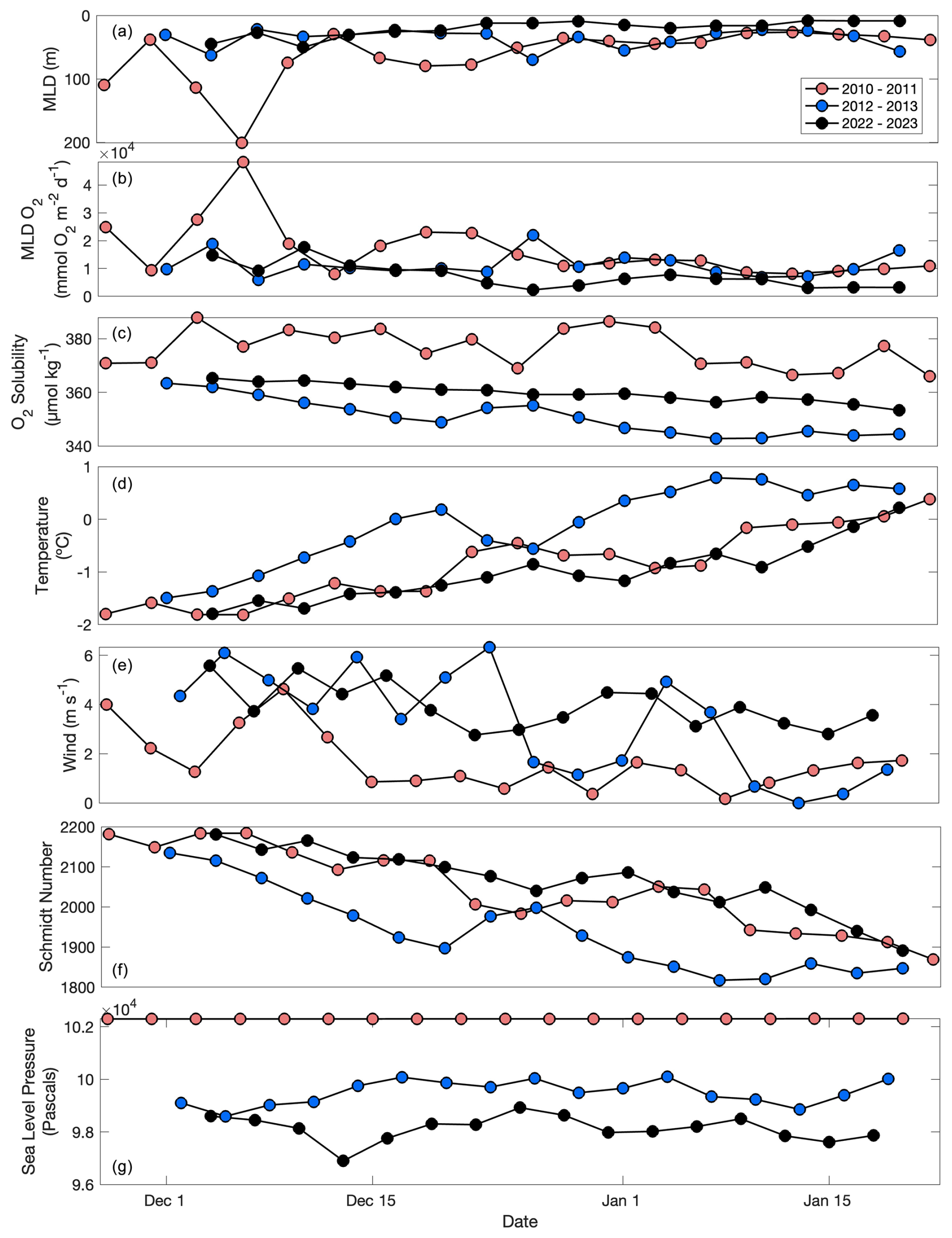
Figure 3 Mixed-layer depth (a; m), mixed-layer integrated dissolved oxygen (b; mmol O₂ m⁻² d⁻¹), oxygen solubility (c; µmol O₂ kg⁻¹), temperature (d; °C), wind (e; m s⁻¹), Schmidt number (f), and sea level pressure (g; pascals) through time for the 2010–2011, 2012–2013, and 2022–2023 deployments. Schmidt number calculations come from Wanninkhof (2014), and wind and sea level pressure are NCEP Reanalysis products. All other parameters come from glider measurements.

POC export potential is the amount of POC available for export in the upper 200 m at the end of the study period. Because each deployment ended before the final bloom succession and biomass export, we measure a potential, rather than actualised export at the end of the deployment period (Hansell and Carlson, 1998; Sweeney et al., 2000). Here, POC export potential was estimated as the difference between the two rates:

$$\begin{array}{}\text{(4)}& {\mathrm{export}}_{\mathrm{POC}}^{\ast }=\mathrm{NCP}-{\displaystyle \frac{\partial \mathrm{POC}}{\partial t}}.\end{array}$$

Equation (4) represents a difference from the calculation of POC export due to the non-steady-state nature of the spring bloom period (Cassar et al., 2015). NCP and $\frac{\partial \mathrm{POC}}{\partial t}$ are integrated over different depth thresholds in accordance with practices established by the Martin curve, which assesses export between 100 m and a variable depth Z (Martin et al., 1987).

The coefficient of variation (%) of stocks and rates were assessed by calculating the percent standard deviation of O₂, POC, $\frac{\partial {\mathrm{O}}_{\mathrm{2}}}{\partial t}$, and $\frac{\partial \mathrm{POC}}{\partial t}$ per season according to Eq. (5):

$$\begin{array}{}\text{(5)}& \begin{array}{rl}& \text{coefficient of variation}\left(\mathit{\%}\right)=\\ & \left({\displaystyle \frac{\text{standard deviation}}{\mathrm{mean}}}\right)\cdot \mathrm{100}.\end{array}\end{array}$$

2.3 Uncertainties

One source of uncertainty in our analysis arises from the estimates of advection. In each deployment, the gliders surveyed in various patterns, making repeat observations of the same water masses and thus quantification of POC and O₂ gradients and currents difficult. However, given these surveys occurred during the Ross Sea bloom period, temporal changes are a first-order control on observations, and spatial changes are a secondary control. This is supported by very low rates of F_ADV and spatiotemporal comparison of observations between multiple gliders in 2022–2023 (Fig. S5). Values of F_ADV may also be influenced by the use of DACs averaged over the entire dive rather than the upper 100 m, but given the low F_ADV values relative to NCP, this does not make a substantial difference in the calculation. For example, if the supposed F_ADV is underestimated by 50 %, this only leads to an underestimate of 0.3, 0.7, and 4.0 mg C m⁻² d⁻¹ in our calculations for 2010–2011, 2012–2013, and 2022–2023, respectively.

Our analysis hinges on the assumption that bio-optical proxies represent their assumed biogeochemical parameter accurately. Because POC and chlorophyll a concentrations were validated in situ, this assumption is valid. Oxygen concentrations were only factory-calibrated and thus likely include higher uncertainty (Bittig et al., 2018). Propagation of uncertainty for all biogeochemical rate measurements was calculated following the method of Yang et al. (2017). We used the offset (i.e. the y intercept) between glider and CTD oxygen optodes and fluorometers to calculate the uncertainty associated with oxygen and POC concentrations (Fig. S1). For the K_z and Schmidt number, we used the previously reported uncertainties of ±7 %–10 % from Yang et al. (2017). This led to mean NCP uncertainties ranging from ±76 % to ±94 %, $\frac{\partial \mathrm{POC}}{\partial t}$ uncertainties ranging from ±38 % to ±45 %, and ${\mathrm{export}}_{\mathrm{POC}}^{\ast }$ uncertainties ranging from ±47 % to ±61 % across each season.

3 Results

3.1 Net community production

Rates of NCP in 2022–2023 were highly variable but suggest net autotrophy with a deployment-wide mean (± standard deviation of all 3 d periods) of 0.2 ± 3.2 g C m⁻² d⁻¹ (Fig. 4a). This value is highest of the three deployments – higher than the mean of −0.7 ± 4.6 g C m⁻² d⁻¹ in 2012–2013 and somewhat higher than the 2010–2011 deployment mean of 0.1 ± 3.8 g C m⁻² d⁻¹ (Fig. 4a). The 2022–2023 season was highly variable, consistent with previous deployments (Fig. 4a). Additionally, the magnitudes of NCP in each deployment were high with approximately half (50 %, 48 % and 63 % for 2010–2011, 2012–2013, and 2022–2023, respectively) of NCP 3 d rates greater than 1.5 g C m⁻² d⁻¹ or less than −1.5 g C m⁻² d⁻¹. The 2010–2011 season exhibited the single greatest productivity event in mid-December when NCP, driven by $\frac{\partial {\mathrm{O}}_{\mathrm{2}}}{\partial t}$, reached 13.0 g C m⁻² d⁻¹ (Fig. 4a). This one 3 d period increased the seasonal average by 0.6 g C m⁻² d⁻¹, moving it from slightly heterotrophic (−0.5 g C m⁻² d⁻¹) to solidly autotrophic. In all three deployments, NCP was driven by $\frac{\partial {\mathrm{O}}_{\mathrm{2}}}{\partial t}$, reinforcing the notion that biological processes are the largest driver of changes in upper-ocean oxygen content during the bloom period, evidenced by this term being an order of magnitude greater than any of the other terms in the oxygen budget (Figs. 5a, 6, S6, S7). Despite the substantial temporal variability between the 3 d periods and negative average NCP observed in 2012–2013, our findings suggest that the Ross Sea is capable of high rates of production.

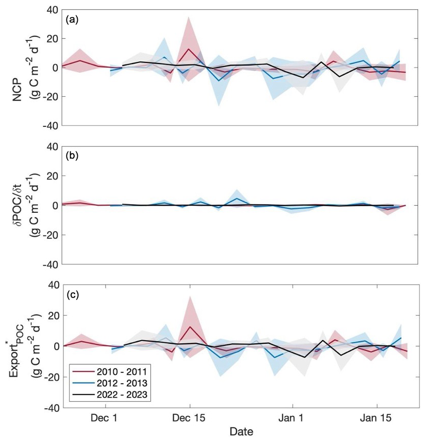
Figure 4 Net community production (a), $\frac{\partial \mathrm{POC}}{\partial t}$ (b), and ${\mathrm{export}}_{\mathrm{POC}}^{\ast }$ (c) through time for glider deployments occurring in the 2010–2011, 2012–2013, and 2022–2023 productive seasons. Units for all rates are g C m⁻² d⁻¹. Shaded regions represent uncertainty for each rate. For NCP, positive values indicate autotrophy, and negative values indicate heterotrophy. For $\frac{\partial \mathrm{POC}}{\partial t}$, positive indicates an increase in POC through time, whereas negative indicates a decrease.

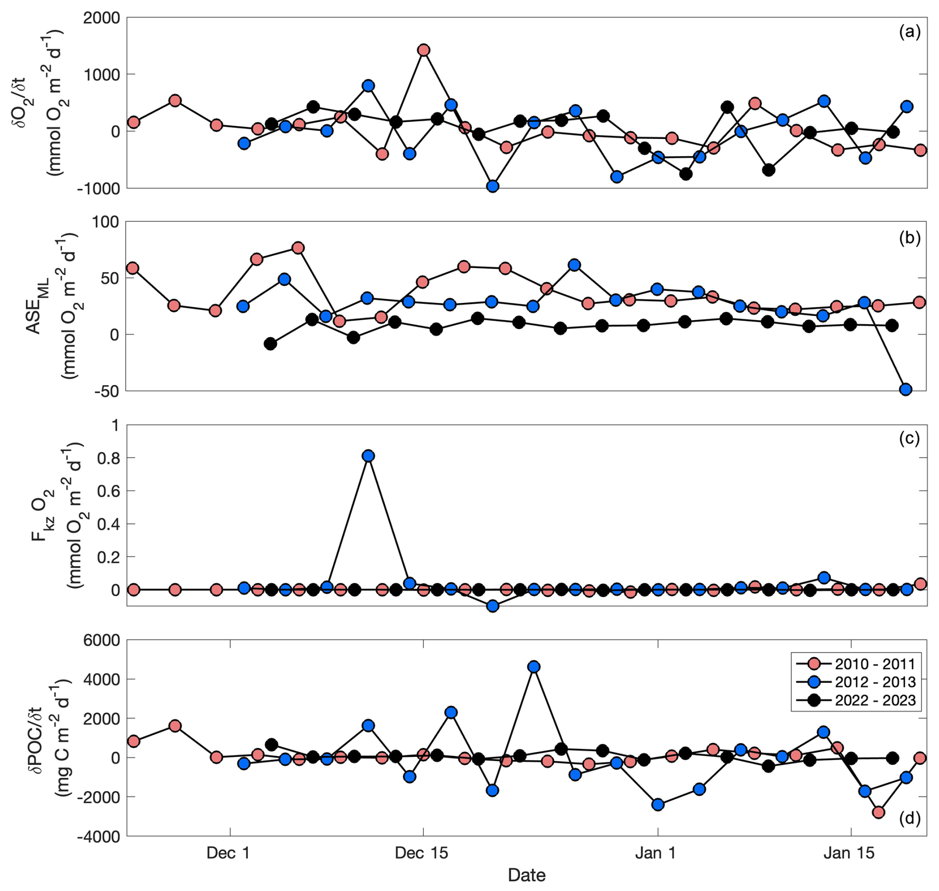
Figure 5 $\frac{\partial {\mathrm{O}}_{\mathrm{2}}}{\partial t}$ (a; mmol O₂ m⁻² d⁻¹), ASE_ML (b; mmol O₂ m⁻² d⁻¹), $F_{K_z}$ O₂ (c; mmol O₂ m⁻² d⁻¹), and $\frac{\partial \mathrm{POC}}{\partial t}$ (d; mg C m⁻² d⁻¹) by day for the 2010–2011, 2012–2013, and 2022–2023 glider deployments. Note the different scales between the y axes.

The individual components of NCP (particularly, $\frac{\partial {\mathrm{O}}_{\mathrm{2}}}{\partial t}$ and ASE_ML) varied substantially between years (Fig. 5). Due to the bloom, $\frac{\partial {\mathrm{O}}_{\mathrm{2}}}{\partial t}$ was the largest component in each year with the highest average rate occurring in 2010–2011 (48 ± 410 mmol O₂ m⁻² d⁻¹; Fig. 5a). ASE_ML was greatest (36 ± 18 mmol O₂ m⁻² d⁻¹) in 2010–2011, consistent with the deepest mixed layers during this year, suggesting that stronger winds that year are responsible for both (Figs. 4b, 5e). ASE_ML was likewise large (26 ± 22 mmol O₂ m⁻² d⁻¹) in 2012–2013 when winds were strong (Figs. 3e, 5b; Meyer et al., 2022a). In all deployments, $F_{K_z}$ made a negligible contribution to total NCP (< 0.01 %–0.1 %; Fig. 5c, d). F_ADV was also low with deployment-wide averages of 7.3 × 10⁻³, −0.1, and 1.4 mmol O₂ m⁻² d⁻¹ for 2010–2011, 2012–2013, and 2022–2023, respectively.

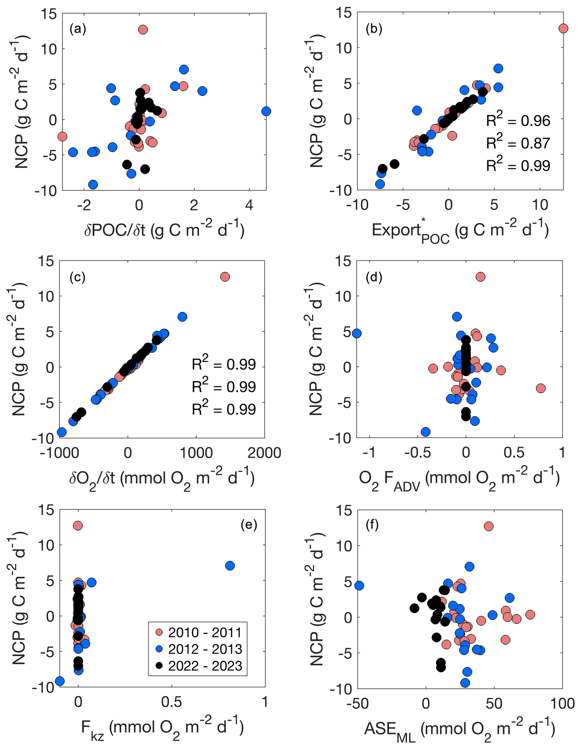
Figure 6 Net community production (NCP; g C m⁻² d⁻¹) versus biogeochemical rates ($\frac{\partial \mathrm{POC}}{\partial t}$, ${\mathrm{export}}_{\mathrm{POC}}^{\ast }$; g C m⁻² d⁻¹) and components of NCP ($\frac{\partial {\mathrm{O}}_{\mathrm{2}}}{\partial t}$, O₂ F_ADV, F_Kz, and ASE_ML; mmol O₂ m⁻² d⁻¹) per day for 2010–2011, 2012–2013, and 2022–2023 glider deployments. R² values indicate correlation coefficients.

3.2 Changes in POC through time

$\frac{\partial \mathrm{POC}}{\partial t}$ and the relationship between $\frac{\partial \mathrm{POC}}{\partial t}$ and NCP behaved differently among deployments (Figs. 5, 6). $\frac{\partial \mathrm{POC}}{\partial t}$ was highest in 2022–2023 when NCP was likewise highest, but POC concentrations were lower during this season than in 2012–2013 (Meyer et al., 2022a; Portela et al., 2025; Fig. 2). The mean 2012–2013 $\frac{\partial \mathrm{POC}}{\partial t}$ rate was similar in magnitude (−0.05 ± 1.7 g C m⁻² d⁻¹) to that of 2022–2023 despite 2012–2013 having a substantially lower NCP rate than in 2022–2023 (Fig. 4b). Like with oxygen, advection of POC was negligible across seasons (averages were 4.3 × 10⁻³, −0.4, and 4.3 mg C m⁻² d⁻¹ for 2010–2011, 2012–2013, and 2022–2023, respectively) and, thus, did not contribute substantially to calculations of $\frac{\partial \mathrm{POC}}{\partial t}$ (Fig. 5f). Compared with NCP, rates of $\frac{\partial \mathrm{POC}}{\partial t}$ per season were all low, suggesting that during the observation period, high rates of production are not matched by high rates of POC removal.

3.3 POC export potential

The temporal variability in ${\mathrm{export}}_{\mathrm{POC}}^{\ast }$ is largely driven by the 3 d temporal variability in NCP (Fig. 4c). Thus, as expected, ${\mathrm{export}}_{\mathrm{POC}}^{\ast }$ rates were highest in 2022–2023 (0.2 ± 3.1 g C m⁻² d⁻¹) and lowest in 2012–2013 (−0.6 ± 3.9 g C m⁻² d⁻¹). In 2023, ${\mathrm{export}}_{\mathrm{POC}}^{\ast }$ from 1 to 3 January was one of the lowest in magnitude observed across all three deployments at −7.2 g C m⁻² d⁻¹ (Fig. 4c). This value was driven by negative NCP and suggests substantial rates of loss processes. Due to its low mean $\frac{\partial \mathrm{POC}}{\partial t}$, ${\mathrm{export}}_{\mathrm{POC}}^{\ast }$ in 2010–2011 (0.1 ± 3.7 g C m⁻² d⁻¹) was comparable to NCP, reinforcing the idea of biomass accumulation in the surface ocean through time during this season. ${\mathrm{export}}_{\mathrm{POC}}^{\ast }$ was also greater than NCP in 2012–2013 but is driven by a variable, frequently negative NCP with biomass accumulation during the observation period, leading to negative average NCP, $\frac{\partial \mathrm{POC}}{\partial t}$, and ${\mathrm{export}}_{\mathrm{POC}}^{\ast }$. Like NCP, our average ${\mathrm{export}}_{\mathrm{POC}}^{\ast }$ is quite high, comparable to 68 %–100 % of the total NCP on average. This finding suggests that substantial POC existed within the top 240 m of the water column but was not removed (e.g. through sinking, grazing, remineralisation) during our observation period.

3.4 Stock and rate variability

As is evident by the large standard deviations on all 3 d means of stocks (O₂, POC) and rates (NCP, $\frac{\partial \mathrm{POC}}{\partial t}$), variability appears to be an important consideration when assessing potential drivers and temporal differences between the parameters of interest. Because the glider and water masses are both moving, the variability evaluated here represents both seasonal spatial and temporal variability of stocks and rates. When evaluated seasonally, spatial variability will be averaged, and temporal variability is likely to be dominant due to the evolution of the bloom (Fig. S5). Substantial variability of POC and O₂ concentrations themselves is not diagnostic of substantial variability in rate patterns. However, an inverse relationship is apparent between variability, in the form of coefficients of variation, of $\frac{\partial {\mathrm{O}}_{\mathrm{2}}}{\partial t}$ and NCP. The highest magnitude of coefficient of variation (−1.1 × 10³ %) coincides with the lowest NCP in 2012–2013, and the lowest magnitude of the coefficient of variation (780 %) coincides with highest NCP in 2022–2023 (Fig. 7).

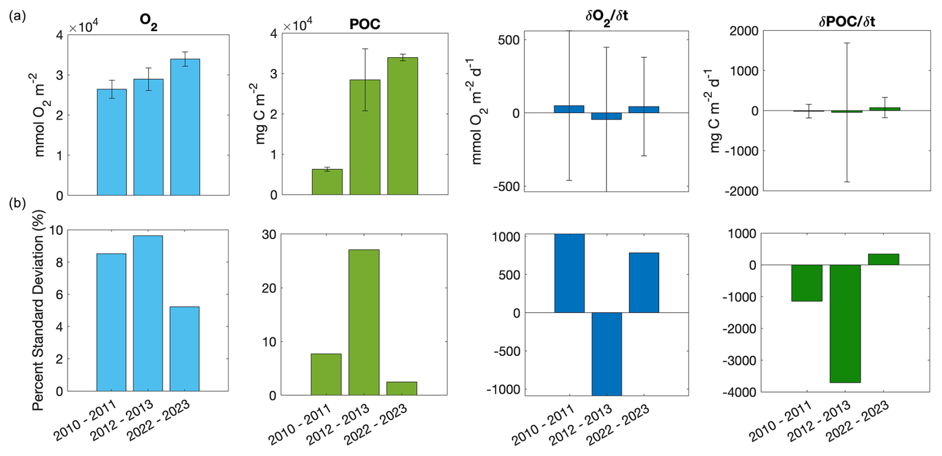
Figure 7 Averages and standard deviations (a) and coefficients of variation (b; all units are %) for dissolved oxygen (mmol O₂ m⁻²), particulate organic carbon (POC; mg C m⁻²), $\frac{\partial {\mathrm{O}}_{\mathrm{2}}}{\partial t}$ (mmol O₂ m⁻² d⁻¹), and $\frac{\partial \mathrm{POC}}{\partial t}$ (mg C m⁻² d⁻¹) for the 2010–2011, 2012–2013, and 2022–2023 deployments.

The variability analysis also highlights some key discrepancies between the mean concentration of parameters between years versus changes through each season and how these relate to the biogeochemical rates of interest (Fig. 7). The time mean of depth-integrated dissolved oxygen concentrations and POC concentrations exhibited different patterns relative to $\frac{\partial {\mathrm{O}}_{\mathrm{2}}}{\partial t}$ and $\frac{\partial \mathrm{POC}}{\partial t}$ (i.e. years with the highest or lowest dissolved oxygen or POC concentrations did not correspond to years with the highest $\frac{\partial {\mathrm{O}}_{\mathrm{2}}}{\partial t}$ or $\frac{\mathrm{POC}}{\partial t}$). Highest mean integrated dissolved oxygen concentrations (3.4 × 10⁴ ± 1.8 × 10³ mmol O₂ m⁻² d⁻¹) were observed in 2022–2023 when $\frac{\partial {\mathrm{O}}_{\mathrm{2}}}{\partial t}$ and NCP were highest, but 2012–2013 had higher average oxygen concentrations but a much lower NCP than 2010–2011 (Figs. 2, 4a). Differing patterns were also evident when comparing POC concentrations and $\frac{\partial \mathrm{POC}}{\partial t}$. However, discrete dissolved oxygen and POC exhibited the highest concentrations in 2012–2013 (Fig. 2). The lower-than-average POC concentrations in 2022–2023 are particularly obvious when evaluated as the mean of concentrations at discrete depths (Fig. 8). The increase in difference (to approximately 20 %) between 25 and 50 m average concentrations toward mid-January would suggest that POC is being retained above 50 m. Unlike POC, chlorophyll concentrations were much higher in 2022–2023 than the other 2 years (Fig. 2).

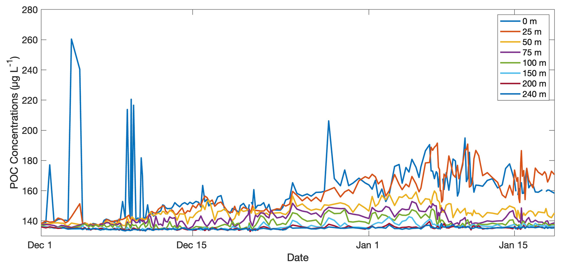
Figure 8 Average particulate organic carbon concentrations (µg C L⁻¹) per depth of interest through time from the 2022–2023 glider deployment. Depths of interest include 0, 25, 50, 75, 100, 150, 200, and 240 m.

4 Discussion

The ability to resolve the surface O₂ and POC fluxes defining these biogeochemical rates at very high spatiotemporal resolution over multiple years provides a better understanding of biological vs. physical controls on the system during the spring bloom. Figure 6 highlights the consistently strong, positive relationship between NCP, $\frac{\partial {\mathrm{O}}_{\mathrm{2}}}{\partial t}$, and ${\mathrm{export}}_{\mathrm{POC}}^{\ast }$ during all deployments. Despite varying rates of O₂ F_ADV, F_Kz, and ASE_ML between deployments, $\frac{\partial {\mathrm{O}}_{\mathrm{2}}}{\partial t}$ is always the dominant term in the upper-ocean dissolved oxygen budget, determining trends in NCP which, in turn, determine trends in ${\mathrm{export}}_{\mathrm{POC}}^{\ast }$ (Figs. 4, 5). Likewise, $\frac{\partial \mathrm{POC}}{\partial t}$ appears consistently uncoupled from NCP (Fig. 6). These findings suggest that, despite substantially varying hydrographic and biogeochemical attributes between seasons, a consistent relationship between production–export dynamics exists between seasons. Thus, our results support the classification of the Ross Sea as a high-production, low-export system (Henson et al., 2019), but the high-resolution data provided by the gliders show substantial 3 d temporal variability during the bloom season that is likely a consistent, yet overlooked, feature of this system. Our results show that this temporal variability impacts rates and our understanding of the relationship between rates when investigated on the subseasonal level.

Our results show that biogeochemical rates and stocks appear uncoupled, with no apparent, strong relationship between NCP and $\frac{\partial \mathrm{POC}}{\partial t}$ rates per season. Seasonal mean NCP varied substantially between years, but seasonal mean $\frac{\partial \mathrm{POC}}{\partial t}$ did not, with the 3 years all within approximately 0.3 g C m⁻² d⁻¹ of each other. This suggests that the variable environmental and biological conditions that lead to substantial differences in NCP are not as strong a control on $\frac{\partial \mathrm{POC}}{\partial t}$ as they are for NCP. Thus, a higher NCP does not necessarily translate to higher $\frac{\partial \mathrm{POC}}{\partial t}$. For example, the low rates of $\frac{\partial \mathrm{POC}}{\partial t}$ in the 2010–2011 season likely stem from the low POC concentrations (Fig. 3) and a variable mixed-layer depth, which could prevent substantial POC accumulation due to mixing-induced light limitation, (Fig. 2a) during this period. Therefore, $\frac{\partial \mathrm{POC}}{\partial t}$ must be kept relatively low by some external factor that was not measured during this study, such as differing lability of P. antarctica versus diatoms (or lack thereof; Misic et al., 2017; Misic et al., 2024) and the role of particle-attached bacteria and remineralisation (Becquevort and Smith, 2001) on backscatter measurements. Coupling glider studies with such analyses should be conducted in future studies as they may help elucidate the mechanism behind consistent $\frac{\partial \mathrm{POC}}{\partial t}$ between seasons.

The ratio of $\frac{\partial \mathrm{POC}}{\partial t}$ to NCP can be considered a proportional POC removal (i.e. how much of the POC that was produced by the bloom during the observation period is removed during the observation period; Fig. 9). The implications of this proportional removal are important for evaluating a system's production–export efficiency. Our results suggest that the proportion of POC removed (Fig. 9) is more important for carbon cycling at times when there is either high NCP and high biomass accumulation as in 2022–2023 or low NCP but high biomass as in 2012–2013, rather than times where there is high NCP but lower biomass as in 2010–2011.

The 2012–2013 glider observations extended into February, approximately 2 weeks longer than the other deployments. When late January and early February rates are included, and values averaged over the entire deployment, NCP is low at 0.05 ± 2.75, whereas $\frac{\partial \mathrm{POC}}{\partial t}$ is much higher at 0.23 ± 1.24 g C m⁻² d⁻¹ (Meyer et al., 2022a). Additionally, these rates were calculated in 5 d intervals, not 3, so some subseasonal variability is likely being smoothed and overlooked due to the longer integration period. This difference in average rates further supports the notion that, due to substantial temporal variability, the timescales over which these rates are averaged are critically important if we want to detect signals of climate change. Thus, establishing our evaluation time frame based on an ecological, rather than temporal, metric (such as chlorophyll concentration) is important and should lead to more biogeochemically reflective rate estimates. These rates are important to compare over the time period when chlorophyll concentrations are greater than 10 % of peak bloom concentrations regardless of the exact days of year.

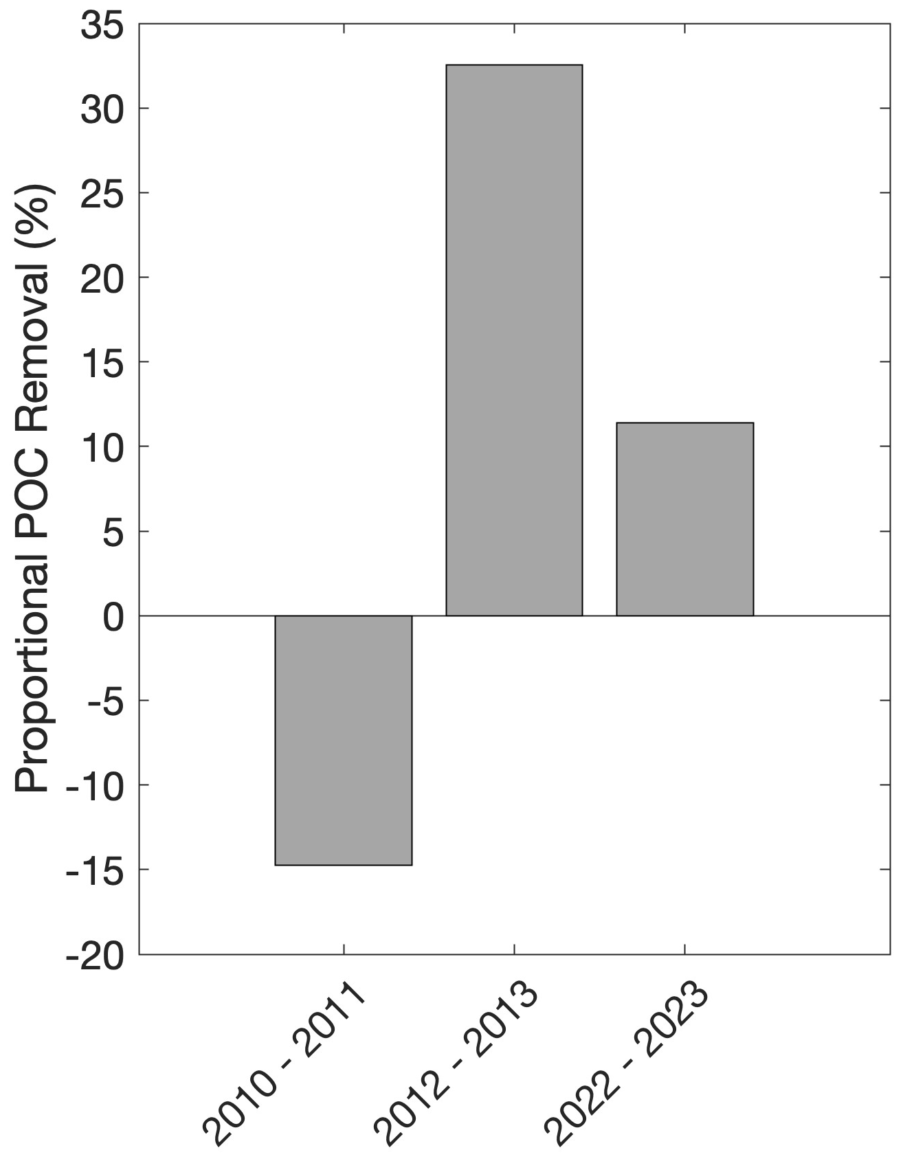
Figure 9 Deployment average proportional POC removal (%; i.e. $\frac{\partial \mathrm{POC}}{\partial t}$ $/$ NCP) per season. Negative values reflect a decoupling of accumulation and removal processes over the course of our study.

This notion of uncoupling between production and export processes is supported by the high retention of POC in the upper water column in 2022–2023 (Fig. 8). Biomass retention is evident by the increasing difference between the mean daily POC concentrations at 25 vs. at 50 m (i.e. POC concentrations at 25 m are up to ∼ 20 % higher than 50 m) from the beginning to the end of the deployment (Fig. 8). Biomass retention is also supported by greater integrated POC concentrations in 2022–2023 (34.0 g C m⁻²) than in 2012–2013 when concentrations declined more from surface to depth (28.4 g C m⁻²; Fig. 2). Some of this difference between years may be taxonomically driven as different phytoplankton groups possess different concentrations of cellular carbon (Rousseau et al., 1990; Smith and Kaufman, 2018), but the daily averaged C : Chl ratios at 5 m, representing the typical surface values, for 2012–2013 and 2022–2023 both increased in late December–early January (Fig. S8). The limited availability of POC and Chl calibration samples prevent us from resolving any specific POC and Chl concentration differences between phytoplankton groups, which may lead to slight under- or overestimations of POC, Chl, and C : Chl ratios as the bloom evolves. Despite this, the dramatic change in C : Chl ratios through time is typical of the annual bloom and suggests a mixed community with a shift from Phaeocystis to diatom dominance over time (Jones and Smith, 2017; Smith and Kaufman, 2018).

Our NCP, $\frac{\partial \mathrm{POC}}{\partial t}$, and ${\mathrm{export}}_{\mathrm{POC}}^{\ast }$ time series (Fig. 4) reinforce the influence of short-term temporal variability on seasonal means on the order of days. This is further emphasised when comparing the 2010–2011 dataset evaluated in this study with a previously published study with a different methodology (Queste et al., 2015). In their study, Queste et al. (2015) calculated daily oxygen changes as the linear regression of apparent oxygen utilisation against time at various depth bins. When evaluating the same period, they found NCP rates ranging from −0.9 to 0.7 g C m⁻² d⁻¹ (Queste et al., 2015). When averaged over the entire deployment, NCP in 2010–2011 from this current study is autotrophic but highly variable at 0.1 ± 3.8 g C m⁻² d⁻¹ (Fig. 4a). This can be attributed to the period from 13 to 15 December, which, due to differences in integration periods for the calculations, appears to be smoothed in the results of Queste et al. (2015) but more apparent in our study. During this period, NCP is 13.0 g C m⁻² d⁻¹, resulting from an exceptionally high $\frac{\partial {\mathrm{O}}_{\mathrm{2}}}{\partial t}$ (1420 mmol O₂ m⁻² d⁻¹; Fig. 5a) but moderate F_ADV, F_Kz, and ASE_ML (0.15, 46, −1.9 × 10⁻³ mmol O₂ m⁻² d⁻¹, respectively). Oxygen concentrations themselves during this time do not appear anomalous (i.e. all dives on 13 to 15 December are internally consistent and within the range observed during 2010–2011), suggesting that this is a real signal with a dramatic (> 4.27 × 10³ mmol O₂ m⁻²) increase over a short period of time (Fig. 5a). Additionally, the oxygen concentrations immediately before 13 December were not anomalously low. Removing the mid-December peak in NCP decreases the 2010–2011 average, making the values similar to those found by Queste et al. (2015). The importance of a singular event to the average 2010–2011 NCP may help explain the substantially lower $\frac{\partial \mathrm{POC}}{\partial t}$ during this season compared with the other two seasons; i.e. a short event does not have as strong an influence in increasing net POC as a consistent period of high NCP. This is likely due to the highly productive nature of the Ross Sea. Other studies have found that in regions of lower average primary production, short-term events have greater net impacts on primary production and/or export (Meyer et al., 2022b). Our study reinforces the influence that integration periods have on results, particularly when analysing NCP during highly dynamic periods (see Niebergall et al. (2023) for a discussion of the role of integration time and space on NCP).

The high NCP observed in 2022–2023 coincides with higher than average chlorophyll a concentrations and a stable water column (Fig. 2; Portela et al., 2025). While surface POC concentrations are lower than the average typically reported for the Ross Sea bloom period (Smith and Kaufman, 2018; Meyer et al., 2022a), depth-integrated POC was high, indicating a substantial accumulation of biomass and retention of that biomass during this season. Portela et al. (2025) provide a more complete discussion of the characteristics and potential drivers of this larger-than-average bloom. The overall characteristics of the 2022–2023 season sharply contrast with the more dynamic, lower-biomass (in terms of both chlorophyll and POC), low-$\frac{\partial \mathrm{POC}}{\partial t}$ 2010–2011 season. Portela et al. (2025) note substantial differences in Ross Sea sea ice concentration, as is evident in Fig. 1, between these 2 years with 2022–2023 having more ice and a later opening of the polynya than 2010–2011 and cite this as a possible mechanism leading to the high chlorophyll concentrations observed in 2022–2023. The influence of sea ice concentration on production through iron seeding, water column stabilisation, and enhanced mixing has been highlighted previously (Arrigo et al., 2008; Smith and Comiso, 2008; Queste et al., 2015).

Current ecosystem models predict that due to alleviation of light limitation, increases in iron concentration, and warmer temperatures, primary production and phytoplankton biomass in the Southern Ocean generally may increase (Moreau et al., 2015; Ferreira et al., 2024). Trends in Ross Sea sea ice cover have varied substantially over the last few decades, showing changes which are frequently masked in compilations of the entire Southern Ocean (Turner et al., 2022). This makes accurate projections of the direction and magnitude of change for future Ross Sea ice cover difficult. Contrary to some studies, our findings suggest that heavy ice cover may, at least temporarily, increase rates of primary production and phytoplankton biomass (Portela et al., 2025). Alternatively, some studies suggest that reduced ice cover will increase long-term primary production due to the alleviation of light limitation, warmer temperatures, and increased nutrient availability (Thomalla et al., 2023). Regardless, our study suggests that an increase or decrease in primary production and POC concentrations in coming decades does not necessarily induce substantial changes in carbon export in the Ross Sea. More research is needed to fully elucidate the fate of POC in the late bloom season in the Ross Sea.

5 Conclusions

When compared with global averages, high-resolution data from three glider deployments support the classification of the Ross Sea as a high-production, low-export system. Our data highlight temporal uncoupling between biogeochemical stocks (POC, O₂) and rates (NCP, $\frac{\partial \mathrm{POC}}{\partial t}$, ${\mathrm{export}}_{\mathrm{POC}}^{\ast }$) and between related rates (NCP and $\frac{\partial \mathrm{POC}}{\partial t}$) when evaluated on short-term (3 d) and seasonal scales during three spring bloom periods. Much of this uncoupling relates to substantial variability which drives rates and reinforces the need for high-resolution measurements. While all three deployments warrant additional observations into the autumn to document the bloom demise and diatom reduction, the implications for production–export dynamics during the peak productive period are clear: high NCP leads to high ${\mathrm{export}}_{\mathrm{POC}}^{\ast }$, and low NCP leads to low or even negative ${\mathrm{export}}_{\mathrm{POC}}^{\ast }$ regardless of the average surface POC and O₂ concentrations during the bloom. These findings should be considered when using just stock concentrations to investigate these dynamics in the Ross Sea.