Fusion of Lagrangian drifter data and numerical model outputs for improved assessment of turbulent dispersion

Transport and dispersion processes in the ocean are crucial, as they determine the lifetime and fate of biological and chemical quantities drifting with ocean currents. Due to the complexity of the coastal ocean environment, numerical circulation models have difficulties to accurately simulate highly turbulent flows and dispersion processes, especially in highly energetic tidal basins such as the eastern English Channel. A method of improving the results of coastal circulation modeling and tracer dispersion in the Dover Strait is proposed. Surface current velocities derived from Lagrangian drifter measurements in November 2020 and May 2021 were optimally interpolated in time and space to constrain a high-resolution coastal circulation MARS model, with careful attention given to selecting ensemble members composing the model covariance matrix. The space–time velocity covariances derived from model simulations were utilized by the optimal interpolation algorithm to determine the most likely evolution of the velocity field under constraints provided by Lagrangian observations and their error statistics. The accuracy of the velocity field reconstruction was evaluated at each time step. The results of the fusion of model outputs with surface drifter velocity measurements show a significant improvement (by ∼ 50 %) of the model capability to simulate the drift of passive tracers in the Dover Strait. Optimized velocity fields were used to quantify the absolute dispersion in the study area. The implications of these results are important, as they can be used to improve existing decision-making support tool or design new tools for monitoring the transport and dispersion in a coastal ocean environment.

1 Introduction

Numerous studies have emphasized the significance of sub-mesoscale O (1–10 km) variability of ocean circulation, which appears highly energetic and ageostrophic. Such sub-mesoscale motions have a notable impact on energy cascade and energy dissipation in the ocean (Ferrari and Wunsch, 2009), as well as on horizontal transport of suspended matter (Aleskerova et al., 2019) or budgets of physical and biological quantities (Uchida et al., 2020). Keerthi et al. (2022) demonstrated that the annual changes in phytoplankton biomass in the Gulf of Mexico are driven by small-scale physical processes (eddies, atmospheric storms, etc.), which control growth and spatial distribution of phytoplankton, and are influenced by the exchange of energy and matter between the atmosphere and the ocean. Both models and observations indicate that the dispersal rate in the presence of sub-mesoscale turbulence can easily exceed the mesoscale dispersal rate in the geostrophic current by an order of magnitude (Haza et al., 2008; Poje et al., 2014).

Incomplete knowledge of forcings in combination with the complexity of coastal environments, which includes a complex shoreline, river mouths, beaches, submarine banks, etc., presents a real challenge for numerical modeling. As a result, circulation models have difficulties in simulating a highly turbulent coastal flow at sub-mesoscale. Hence, it is important to develop techniques that can improve the model skill to reconstruct the water circulation and dispersion processes in coastal environments in a simple and efficient way.

The current study employs a method of optimal interpolation (OI) of Lagrangian observations using a high-resolution regional circulation model as a background. Lagrangian observations of current velocities are used to correct the model trajectories in an optimal way. Pioneered by Gandin (1963) and applied in atmospheric modeling, the OI has been widely used in different fields of geosciences for mapping the sea surface temperature (Bretherton et al., 1976), modeled current velocity optimization (Molcard et al., 2003; Sentchev and Yaremchuk, 2015), and topography optimization (Wu et al., 2021). Compared to other approaches to optimizing ocean circulation such as variational methods (e.g., Kalnay, 2002; Sentchev and Yaremchuk, 1999; Wikle, 2005), the OI has several advantages. Firstly, the method is straightforward to implement and ensures a reasonable balance between the computational complexity and statistical consistency of the model–data misfits. Secondly, the accuracy of the reconstructed velocity field can be inexpensively evaluated at every time step of the model.

The use of OI of observations leads to a significant improvement of the current velocity fields and velocity gradients, which are often inadequately represented in the models due to their low resolution or intrinsic limitations. Therefore, the turbulent dispersion also appears to be affected by these limitations. Many studies have focused on the investigation of processes that influence the dispersion in the ocean, such as tidal motions (Meyerjürgens et al., 2020), waves (Weichman and Glazman, 2000), and the variability of ocean circulation (Haza et al., 2008; LaCasce and Ohlmann, 2003; Lumpkin and Elipot, 2010). The present study aims to quantify the effect of current velocity optimization on the dispersion rate of passive tracers in a tide-dominated region: the Dover Strait, in the eastern English Channel (EEC).

The paper is organized as follows: Sect. 2 provides a general presentation of the study area and the data used. Section 3 provides a detailed description of the methods utilized in this study. The results of OI of Lagrangian measurements and characterization of dispersion processes are presented in Sect. 4. Furthermore, a technique for correcting the wind-driven velocity component of surface currents is proposed in Sect. 4. Discussion and conclusions are presented in Sects. 5 and 6, respectively.

2 Study site and the data

2.1 Study site and hydrodynamic conditions

The study was carried out in the Dover Strait, a shallow-water region of the northwestern European continental shelf connecting the English Channel to the North Sea (Fig. 1a). The region is characterized by highly irregular bathymetry, with depth not exceeding 65 m and the presence of many sandbanks, roughly oriented in the dominant current direction, with depth only of a few meters at low tide.

Tidal motions of semi-diurnal periods dominate the local circulation. The tidal range in Boulogne, located on the eastern coast of France (Fig. 1a), is close to 9 m, and the current speed can reach 2 m s⁻¹ during spring tide. The tidal stream loses around 20 % of its intensity during ebb tide, and the sea surface height and velocity are characterized by a pronounced asymmetry. A large-scale circulation in the North Atlantic Ocean generates sea level difference, driving a weak residual flow from the Atlantic Ocean towards the North Sea. This is another remarkable feature of the local hydrodynamics. The order of magnitude of the tidal residual currents in the Dover Strait ranges between 5 and 10 cm s⁻¹ (Lazure and Desmare, 2012). The spatial variability of residual currents is caused by topographic features of the English Channel that constrain tidal wave propagation (e.g., Sentchev and Yaremchuk, 2007).

The wind significantly affects the local circulation. Southwestern winds can increase the average eastward flow, while northwestern and northeastern winds can reduce the tidal flow opposing the wind and even reverse it (e.g., Lazure and Desmare, 2012). The freshwater input from rivers located on the French coast (the Seine, the Somme, and the Authie rivers) has only a little influence on the water circulation in the study area.

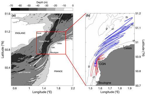
Figure 1 (a) Modeling domain. Bathymetry shown by grey shading. Red square delimits the region where the Lagrangian measurements were performed. (b) Trajectories of Lagrangian drifters released during two field surveys on 26 November 2020 (red) and on 10 May 2021 (blue). Geographic names used in the text are also shown.

2.2 Current velocity measurements

A total of six Lagrangian surface drifters were deployed in the Dover Strait during two periods of time, under relatively calm to moderate winds (mean wind speed less than 8 m s⁻¹) and waves not exceeding 1 m height. During the first survey, referred to hereafter as S1, two surface drifters were released north of the Cap Gris-Nez (CGN) (Fig. 1b, red trajectories) for a 26 h period, from 26 November 2020 at 08:30 UTC to 27 November 2020 at 11:00 UTC. At the release, the two drifters were separated by 250 m. The survey was performed under mean tide conditions and northeastern wind of 4 m s⁻¹, on average. The two drifters of S1 will be referred to hereafter as S1-1 and S1-2. During the second survey, referred to hereafter as S2, four surface drifters were deployed west of the CGN (Fig. 1b, blue trajectories) for a 46 h period, from 10 May 2021 at 09:15 UTC to 12 May 2021 at 07:30 UTC. The drifters formed a rectangle of size of 1.3 km by 2 km. The survey was performed under spring tide conditions and stronger southwestern winds of 6 m s⁻¹, on average, with gusts up to 12 m s⁻¹. The four drifters of S2 will be referred to hereafter as S2-1, S2-2, S2-3, and S2-4.

Two types of buoys were used: coastal Nomad surface buoys manufactured by SouthTek (https://www.southteksl.com/, last access: 15 January 2024) and drifters manufactured at the lab. The coastal Nomad buoy is a cylinder 0.72 m long and 0.22 m wide with a cone positioned at the surface to increase buoyancy. The laboratory-made drifter comprises a cylindrical PVC hull 0.6 m long and 0.1 m in diameter weighted in its lower part. A thin square plate of 0.3 × 0.3 m in size was installed in the upper part of the hull to assure better stability in the vertical and reduce the pitch. The drifters were equipped with a SmartOne GPS/satellite transceiver of Globalstar satellite network. All drifters were equipped with a 0.5 m long floating anchor positioned in the water layer at 1 m depth, allowing them to drift with surface currents. For this study, we assumed that SouthTek drifters and laboratory-made drifters behaved similarly at sea and that the discrepancies implied by their differences were negligible.

Observed surface current velocities were estimated from the drifter trajectories with a time step of 15 min, which was a nominal period of drifter positioning via GPS. Spatial coordinates (longitude, latitude) were obtained and then derived and divided by the time step to estimate the velocity at each time step.

During S1, the mean drifter velocity was 0.8 m s⁻¹. The maximum speed of 1.6 m s⁻¹ was reached during peak flood flow and observed north of the CGN. The minimum speed of 0.1 m s⁻¹ was reached 2 h after peak ebb flow and observed south of the CGN. During S2, the mean and maximum drifter velocities were found to be 1 and 2.1 m s⁻¹ respectively (Fig. 1a).

2.3 Current velocity from numerical model

The water dynamics in the EEC are largely dominated by tides. The baroclinic effects on the vertical are negligible due to the enhanced mixing affecting the entire water column (e.g., Breton and Salomon, 1995). Moreover, the study area is located fairly far away from the major source of buoyancy – the Seine River, whose discharge was low during the measurement period. The use of a 2D model was therefore justified. The variation of salinity in the horizontal plan is taken into account in the 2D model.

Lagrangian particle advection simulations performed in this study were forced by a 2D water current (barotropic) and water level forecasts modeled in the framework of the operational coastal oceanography project Modeling and Analysis for Coastal Research (Pineau-Guillou, 2013; Dumas et al., 2014). The forecasting multi-scale real-time and historical data for the French metropolitan coastlines including the eastern English Channel are freely available on their project website (https://marc.ifremer.fr, last access: 12 October 2023). Current, salinity, temperature, and sea level elevation fields were forecasted using the Model for Application at Regional Scale (MARS) (Lazure and Dumas, 2008).

The MARS model was developed to simulate flows across various coastal areas, ranging from regional scales to the inshore scale of small bays or estuaries, where circulation is typically influenced by a combination of processes (Lazure and Dumas, 2008). The modeled processes involve simplifications of the incompressible Reynolds-averaged Navier–Stokes (RANS) equations based on classic Boussinesq and hydrostatic assumptions. Comprehensive information regarding model equations, the coupling of barotropic and baroclinic modes, model discretization, solving methods, computational stability according to the Courant–Friedrichs–Lewy criterion (Table 1; Lazure and Dumas, 2008), and costs is meticulously outlined in Lazure and Dumas (2008). The model accounts for kinematic free-surface and bottom boundary conditions, contingent upon friction terms (Lazure and Dumas, 2008). The turbulence closure employed in the model follows the approach described in Gaspar et al. (1990).

To accurately simulate storm surge dynamics, the model extends sufficiently to the north and west to capture the development of depressions, which generate surges propagating in the English Channel at a greater distance in the Atlantic Ocean or in the North Sea (Idier et al., 2012). The numerical model utilizes nested configurations with progressive resolutions: (i) 2 km covering the northeastern Atlantic (level 0); (ii) 700 m at the regional scale, encompassing the English Channel (level 1); and (iii) 250 m for the eastern English Channel (level 2). This nesting technique enables the accurate capture of interactions between large-scale and small-scale processes. This technique enables the transfer of all resolved fields from lower-resolution levels to the open boundaries of higher-resolution levels. The temporal resolution of the outputs is 1 h for levels 0 and 1 and 15 min for level 2.

All relevant details concerning the choice of bathymetry, meteorological and tidal forcings, improvements in model parameterization (such as surface friction and drag coefficient), and the methodology employed for storm-surge computation are meticulously documented in Pineau-Guillou (2013). The bathymetry data for the level-2 configuration were sourced from the French Hydrographic and Oceanographic Service (SHOM). Tidal boundary conditions were derived from the global tidal model FES2004 (Lyard et al., 2006). Intertidal areas were simulated using a wetting and drying scheme. The drag coefficient utilized for wind effect parameterization is based on the variable Charnock coefficient from the WaveWatch III model (Ardhuin et al., 2011). To maintain CFL stability, the modeling time step was set to 30 s for the level-2 model.

Moreover, the numerical model outputs underwent an evaluation process (Pineau-Guillou, 2013; Dumas et al., 2014) involving available observations, confidence indicators, and descriptors of system states. Regarding the water levels, the model was validated in February 2010 at 19 tide gauges of the permanent network RONIM (French Sea Level Observation Network). For the tide, the root mean square errors are halved between level 0 and level 2: they average 22 cm for level 0, 21 cm for level 1, and 11 cm for level 2. Similar results are observed for the water levels (tide and surge) with root mean square errors averaging 26 cm for level 0, 24 cm for level 1, and 16 cm for level 2. These improvements are attributed to the enhancement of spatial resolution from level 0 to level 2 (from 2 km to 250 m), as well as the incorporation of the SHOM CST-France tidal model (with 115 harmonic components) at the boundaries of the model (Pineau-Guillou, 2013).

Hence, we posit that the comparison of model outputs for the level-2 configuration (with 250 m horizontal spatial resolution and 15 min output temporal resolution), encompassing the EEC area with available in situ data, is sufficiently accurate to be utilized in our study for further drifting particle advection modeling. Originally represented on an Arakawa C-grid, surface currents were interpolated on the Arakawa A-grid (Arakawa and Lamb, 1977) for further analysis and optimization of model velocities. The model used in the analysis will be referred to hereafter as M2D.

2.4 Wind data

Meteorological data (wind, temperature, humidity, and atmospheric pressure) are used as the forcing of M2D. The data were provided by the Arpege (Action de Recherche Petite Echelle Grande Echelle) operational atmospheric model of Météo-France with 5 km spatial and 1 h time resolution.

The meteorological data from the model were compared to in situ measurements collected at meteorological station in Boulogne and Calais during the year of model simulations. The time- and space-averaged difference between the observed and modeled wind speed was found to be 1.7 and 0.9 m s⁻¹ for the surveying periods, giving confidence in the model wind data.

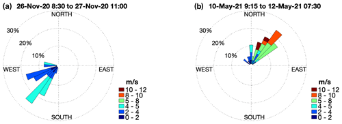
Figure 2 Wind roses for two survey periods: S1 (a) and S2 (b) from the Arpege atmospheric model (hourly data) spatially averaged over the study region.

Figure 2 shows the wind rose for each survey from the Arpege model. Two dominant wind regimes were observed during the surveyed days. During S1, the wind direction was towards the southwest, and the speed did not exceed 5 m s⁻¹ with the mean value of 4 m s⁻¹. During S2, the wind had an opposite direction, and the speed varied within the range of 4–9 m s⁻¹, with the mean speed 6 m s⁻¹ and the maximum speed 11 m s⁻¹.

3 Methodology

3.1 Optimal interpolation of velocity measurements

One of the methods used to constrain the numerical model outputs by observations is the optimal interpolation of observations. It provides an estimate of the state of the ocean dynamics by performing a weighted least squares fit of a background model field to observations. In general, observations are available at irregularly distributed points and are assumed to be imperfect, i.e., each observation being affected by an uncertainty (observation error). It is assumed that the observation error is not correlated with the model error.

In the OI method, a correction of a background velocity field u_m(x,t), provided by a numerical model on a regular grid, is done using a linear combination of the weighted differences between the background model velocity u_m and the observed velocities ${\mathit{u}}_i^{\ast }$ at point i (Bretherton et al., 1976; Sentchev and Yaremchuk, 2015; Thiébaux and Pedder, 1987). Weights chosen for minimization of the mean square difference between the observed and background velocities are a combination of model and observation covariances. With the space–time covariance matrices of the model $\mathbf{B}=〈{\mathit{u}}_{\mathrm{m}}\left(\mathit{x},t\right){\mathit{u}}_{\mathrm{m}}\left({\mathit{x}}^{\prime },t^{\prime }\right)〉$ and observations ${\mathbf{R}}_{ij}=〈{\mathit{u}}_i^{\ast }{\mathit{u}}_j^{\ast }〉$, the optimized velocities u_OI are computed as follows:

$$\begin{array}{}\text{(1)}& {\mathit{u}}_{\mathrm{OI}}={\mathit{u}}_{\mathrm{m}}+\sum _{ij}{\mathbf{BH}}_j^{\mathrm{T}}{\left({\mathbf{H}}_i{\mathbf{BH}}_j^{\mathrm{T}}+{\mathbf{R}}_{ij}\right)}^{-\mathrm{1}}\left({\mathbf{H}}_i{\mathit{u}}_{\mathrm{m}}-{\mathit{u}}_i^{\ast }\right).\end{array}$$

Here, H_i corresponds to a linear operator projecting gridded velocity values from the apexes of the model grid cell onto the ith observation point. The covariance of u_m is calculated between space–time coordinates (x,t) and $\left({\mathit{x}}^{\prime },t^{\prime }\right)$, where x and t correspond to the velocity and time of observations, and x^′ and t^′ are the corresponding velocity and time in the different ensemble members composing the covariance matrix.

The quality of the interpolation scheme is quantified by estimating the mean relative difference between the observations u^∗ and optimized model velocities u_OI as follows:

$$\begin{array}{}\text{(2)}& {\mathit{\epsilon }}_{\mathrm{OI}}=\sqrt{{\displaystyle \frac{\sum _i{\left({\mathbf{H}}_i{\mathit{u}}_{\mathrm{OI}}-{\mathit{u}}_i^{\ast }\right)}^{\mathrm{2}}}{\sum _i{\left({\mathit{u}}_i^{\ast }\right)}^{\mathrm{2}}}}}.\end{array}$$

The relative error of the initial model, ε_m, is quantified in the same way.

An important assumption underlying the OI method is that the background field, also called the “first guess”, is a good approximation of the truth. Thus, the computation of B and u_m is crucial. The background velocity fields were provided by the model at the observation time step.

For estimation of model covariances, a variable number of model trajectories (26 h long for S1 and 46 h long for S2), referred to as ensemble members, were used. The sensitivity test of OI to the number of ensemble members used was performed, and the results are presented in Sect. 4.1. Three approaches were used in selecting the ensemble members. The first and easiest way is extracting them from the model on the days surrounding the survey and by respecting the conditions (wind and tidal conditions) observed during the surveying days. A total of seven ensemble members were selected using this approach.

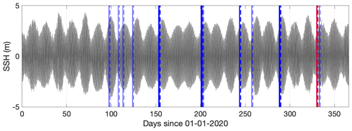
Figure 3 A total of 31 ensemble members (in blue) extracted from the model simulation of circulation in the Dover Strait using the realistic forcing in 2020. S1 period is shown in red. Sea surface height (SSH) from the model run is given in dark grey. Solid lines mark the beginning of the ensemble member, whereas dashed lines mark the end.

However, for an evolving ocean state, a large number of ensemble members might be required to represent the flow field evolution with statistical significance. Therefore, in the second step, ensemble members were extracted from the 1-year-long model simulation (January to December 2020) containing S1, by searching for wind and tidal conditions similar to those observed during the surveying period. By accepting a variation of the average wind speed and direction within the range ±2 m s⁻¹ and ±45° respectively, for a given tidal stage, a total of 31 ensemble members were selected. In a third step, a more restrictive criterion of the range of variation of the wind, for instance, ±1 m s⁻¹ and ±45°, allowed us to obtain 11 ensemble members. Figure 3 shows a chronology of ensemble members selected for OI of velocity observations during S1. Each ensemble member represents a 26 h long model run.

3.2 Lagrangian trajectory reconstruction

In addition to the relative error ε, the quality of the interpolation scheme can be assessed by estimating the separation distance d between the real trajectories of drifting buoys and the trajectories provided by the model. The latter were reconstructed using the OceanParcels Lagrangian framework (https://oceanparcels.org/, last access: 29 October 2023). Virtual particles were seeded at the time and location of the real drifters at the release. Then, they advected during a given period of time using the horizontal forward Euler method without diffusion, giving their time-dependent position x(t) and y(t). The separation distance d, estimated at a 15 min time step and averaged over drifters, is a commonly used metric that shows how good the drifter trajectories are reconstructed by the initial model (the separation distance d_m) or the optimized model (the separation distance d_OI).

3.3 Correction of the wind-induced current velocities

The ocean–atmosphere coupling is difficult to reproduce correctly, especially in coastal regions. In fact, the wind generates surface Ekman currents directed 45° to the right of the wind at the sea surface. It is assumed that this wind-driven velocity can attain 1 %–3 % of the wind speed at 10 m height (Jenkins, 1987; Weber, 1983).

Imperfect representation of the wind-driven velocity in the model can be improved by using velocity measurements by surface drifters. Let us assume that the flow velocity can be decomposed in two parts: the optimally interpolated velocity u_OI and an additional correction, $\mathit{c}{\stackrel{\mathrm{‾}}{U}}_{\mathrm{10}}$, where ${\stackrel{\mathrm{‾}}{U}}_{\mathrm{10}}$ is the wind velocity vector at 10 m height, averaged over the study area and the survey period, and $\mathit{c}=\mathrm{diag}\left(c_x,c_y\right)$ is a diagonal 2×2 matrix whose diagonal elements are estimated by minimizing the cost function:

$$\begin{array}{}\text{(3)}& \begin{array}{rl}J\left(c\right)& ={\left[{\mathbf{X}}^{\ast }-\left({\mathbf{X}}_{\mathrm{0}}+\sum _k{\left({\mathit{u}}_{\mathrm{OI}}\right)}_k\mathrm{\Delta }t+\mathit{c}{\stackrel{\mathrm{‾}}{U}}_{\mathrm{10}}\mathrm{\Delta }t\right)\right]}^{\mathrm{2}}\\ & \to \begin{array}{c}min\\ c\end{array}.\end{array}\end{array}$$

Here X^∗ is a sequence of drifter coordinates at Δt=15 min time stepping, X₀ is the coordinate at the release, and summation is performed over a drifter trajectory. The expression in parentheses represents a virtual drifter trajectory after correction for the wind effect. The coefficients (c_x,c_y) were estimated for each drifter trajectory and then averaged. This implies an assumption of a stationary wind (mainly wind direction) that was supported by observations at meteorological stations during the surveying periods S1 and S2. Correcting the wind-induced velocity enables better reconstruction of the optimized velocity fields denoted hereinafter by u_cor. The relative error of the model after performing the wind-induced velocity correction is computed using Eq. (2), after replacing u_OI by u_cor. The separation distance between the observed trajectories and trajectories reconstructed from the model after performing wind-induced velocity correction is referred to as d_cor.

3.4 Absolute dispersion

The absolute dispersion A² is defined as the variance of particle spreading with respect to the mean coordinate of particles in a cluster (the barycenter). In two-dimensions, the dispersion is generally estimated along the x and y axes (Berti et al., 2011; Enrile et al., 2019). But in this study, to better account for the dominant flow direction, the variance is computed in the direction of the maximum spreading of particles and in the perpendicular direction, providing the two quantities $A_{\mathrm{1}}^{\mathrm{2}}$ and $A_{\mathrm{2}}^{\mathrm{2}}$. They represent the major and minor axes of the deformation tensor and are estimated by applying the principal component analysis (PCA) to particle distribution at each time step (Emery and Thomson, 2004). As the tidal flow direction in shallow-water basins is generally constrained by local topography and coastline orientation, the ellipse orientation (major axis) gives the dominant flow direction. The ellipse orientation θ and the variances $A_{\mathrm{1}}^{\mathrm{2}}$ and $A_{\mathrm{2}}^{\mathrm{2}}$ were computed as follows (Emery and Thomson, 2004):

$$\begin{array}{}\text{(4)}& {\displaystyle }\mathit{\theta }={\displaystyle \frac{\mathrm{1}}{\mathrm{2}}}{\tan }^{-\mathrm{1}}\left[{\displaystyle \frac{\mathrm{2}\stackrel{\mathrm{‾}}{x^{\prime }{y}^{\prime }}}{\stackrel{\mathrm{‾}}{x^{\prime \mathrm{2}}}-\stackrel{\mathrm{‾}}{y^{\prime \mathrm{2}}}}}\right]\text{(5)}& {\displaystyle }\begin{array}{rl}\left.\begin{array}{c}{A}_{\mathrm{1}}^{\mathrm{2}}\\ A_{\mathrm{2}}^{\mathrm{2}}\end{array}\right]& ={\displaystyle \frac{\mathrm{1}}{\mathrm{2}}}\mathit{\{}\left(\stackrel{\mathrm{‾}}{x^{\prime \mathrm{2}}}+\stackrel{\mathrm{‾}}{y^{\prime \mathrm{2}}}\right)\\ & \pm {\left[{\left(\stackrel{\mathrm{‾}}{x^{\prime \mathrm{2}}}-\stackrel{\mathrm{‾}}{y^{\prime \mathrm{2}}}\right)}^{\mathrm{2}}+\mathrm{4}{\left(\stackrel{\mathrm{‾}}{x^{\prime }{y}^{\prime }}\right)}^{\mathrm{2}}\right]}^{\frac{\mathrm{1}}{\mathrm{2}}}\mathit{\}}.\end{array}\end{array}$$

Here, $\stackrel{\mathrm{‾}}{x^{\prime \mathrm{2}}}$ and $\stackrel{\mathrm{‾}}{y^{\prime \mathrm{2}}}$ stand for variances of particle coordinates along the eastward x and northward y axes, respectively.

4 Results

4.1 Model velocities after optimal interpolation of the Lagrangian observations

Figure 4 shows the results of Lagrangian drifter velocity interpolation for S2. The largest number of ensemble members, 36, was used in interpolation. The discrepancy between the initial and optimally interpolated velocities during peak flood and ebb flow (Fig. 4, color shading) varies in space with lower values found south of the CGN, for both flood and ebb flow, and the largest value (∼ 0.5 m s⁻¹) found in the northern part of the strait, close to the UK coast. In the French sector of the strait, the discrepancy attains 0.2 m s⁻¹ over the sandbanks. However, the surface current direction is reproduced fairly well by M2D. The mean (time- and space-averaged) error of flood and ebb tide velocity is 0.17 and 0.25 m s⁻¹, respectively, while for the current direction, the corresponding errors are 2 and 2.5°. In general, larger discrepancies are found over sandbanks, indicating difficulties in modeling the tidal stream over complex and rapidly changing bathymetry.

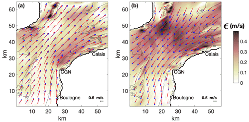
Figure 4 Current velocities during peak flood flow (a) and peak ebb flow (b) of survey S2. Red and blue vectors show the initial and optimized model velocities, respectively. The absolute difference between the initial and optimized model velocity (|u_OI−u_m|) is shown by color shading.

The relative error of velocity, ε, appears significantly different in the initial model and after OI (Table 1). In the initial model, the error (ε_m) is found to be fairly large: 0.27 for S1 and 0.22 for S2. Blending the model with Lagrangian observations allowed a decrease in the relative error by 40 % for S1 and by more than 50 % for S2 (Table 1, columns 2 and 3). The larger error obtained for S1 could be due to the location of drifter trajectories too close to the shore, during 10 h after the release. The model performance in reconstructing the drifter trajectories is probably limited in this very shallow-water region, in the vicinity of the CGN.

It is interesting to quantify the sensibility of OI to the number of ensemble members used. While the number is limited to seven (the smallest number identified for both surveys), the results of velocity interpolation do not change much, by less than 10 % (Table 1, column 3, values in italics). These outcomes prove that in a basin dominated by the combination of tide and wind, and in the EEC in particular, the accuracy of OI is not much sensitive to the number of ensemble members used in calculating the velocity covariances. Note that wind forcing is taken into account when selecting ensemble members. With tidal range varying between 3 and 9 m in the EEC, the correlations of current velocities are high. This may explain why increasing the number of ensemble members results in only a slight decrease in the interpolation error.

Table 1 Relative error ε (columns 2–4) and mean (time–space-averaged) separation distance (columns 5–7) between the observed and reconstructed drifter trajectories, using the initial model, optimized model, and the model after performing wind-induced velocity correction. Errors obtained with 31 ensemble members for S1 and 36 for S2 are shown in normal font, and those obtained with 7 ensemble members are given in italics.

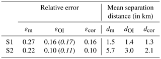
Figure 5 shows the evolution of differences between the velocity provided by the initial and optimized model in drifter locations during S1 (Fig. 5a, b) and S2 (Fig. 5c, d). During S1, larger discrepancies between both the observed–modeled velocities and the observed–optimized velocities (∼0.3 m s⁻¹) occur at peak flood, 13 h after the deployment. However, the optimization enables the reduction of the mean discrepancy from 0.070 to 0.066 m s⁻¹ for u_x and from 0.10 to 0.066 m s⁻¹ for u_y. During S2, larger discrepancies are attained during both peak flood (time 26, 40 h) and peak ebb flow (time 8, 22, 33, 46 h). The optimization process enables the reduction of the mean discrepancy from 0.09 m s⁻¹ down to 0.07 m s⁻¹ for u_x and from 0.07 down to 0.06 m s⁻¹ for u_y. These results highlight the difficulty models have to reproduce accurately the exact timing between peak flood and ebb flow.

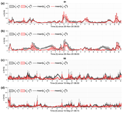
Figure 5 Boxplots of absolute zonal (a, c) and meridional (b, d) velocity difference between observations and initial model (black) and observations and optimized model (red) at S1 (a, b) and S2 (c, d) drifter locations. For S1 (a, b), where only two drifters are considered, the top and bottom edges of each box are the maximum and minimum values, and the line within the box indicates the median, equal to the mean. For S2 (c, d), the top and bottom edges of each box are the upper (0.75) and lower (0.25) quartiles, respectively. The line within the box indicates the median. The whiskers above and below each box are the nonoutlier maximum and minimum.

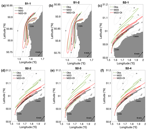
Figure 6 shows the observed drifter trajectory and that provided by the initial and optimized model during S1 and S2. The corresponding separation distance, time- and space-averaged, is given in Table 1 (columns 5–7). During S1, the model seems to underestimate the northward flow component, especially in the southern part of the domain (Fig. 6a, b). The mean initial separation distance d_m is 1.5 km. It decreases by 0.1 km after OI (d_OI=1.4 km). During S2, the model, both initial and optimized, underestimates the northward flow component (Fig. 6c, d, e, and f). The time evolution of the trajectories is well reproduced by the model, especially for drifter of drifter S2-1, but appears shifted by 4 km compared to the observed trajectory. This gives a large mean separation distance d_m=5.7 km. Blending the model with observations enables the reduction of the mean separation distance by 7 % for S1 and by 48 % for S2 (Table 1, columns 4–5). However, the difference between the real and virtual drifter trajectories remains significant, especially for S2 (Fig. 6c, d, e, and f).

Another way to evaluate the performance of OI is to perform a “leave-one-out validation” experiment. In this experiment, one drifter trajectory is removed from the data set, and the optimization is done using the remaining drifters. This validation method provides a much less biased measure of relative error compared to that used in cross-validation, because the model is repeatedly fit to a data set that contains n−1 drifter trajectories. At the end of the experience, the relative error was reduced by 22 % for S1 and by 36 % for S2. This proves the that proposed OI technique is capable of efficiently correcting the few drifter trajectories of the model velocity field. These values of error reduction appear similar to those given in Table 1 and demonstrate the efficiency of the OI. This means that with only one or few drifters, it is possible to improve the model velocities in an optimal way.

Figure 6 Observed trajectory of drifter S1 (a, b) and S2 (c, d, e, f) (green lines). Corresponding trajectories provided by the initial model M2D are shown in black and those resulting from OI in red. Mean wind speed and direction are denoted by a black arrow.

4.2 Wind-induced velocity correction

The fact that larger separation distance between the observed and reconstructed trajectories was obtained during S2 (under strong wind conditions) indicates that the effect of wind on surface currents is poorly reproduced in the model. To further reduce the discrepancy between the observed and modeled trajectory, the least squares method is used to estimate a correction to wind-induced velocity. Figure 7 shows the evolution of the separation distance between the observed and reconstructed drifter trajectories using the initial, optimized, and velocity field after correcting the wind-induced current. The correction term $\mathit{c}{\stackrel{\mathrm{‾}}{U}}_{\mathrm{10}}$ (Eq. 3) was calculated for both zonal and meridional wind components and given as percentage of the wind speed, corresponding to −0.4 % ${\stackrel{\mathrm{‾}}{U}}_{\mathrm{10}}$ and 2.8 % ${\stackrel{\mathrm{‾}}{V}}_{\mathrm{10}}$ during S1 and −0.4 % ${\stackrel{\mathrm{‾}}{U}}_{\mathrm{10}}$ and 1.7 % ${\stackrel{\mathrm{‾}}{V}}_{\mathrm{10}}$ during S2.

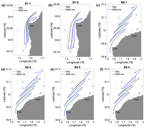
Figure 7a demonstrates that, under certain conditions, the wind-induced velocity correction is not effective. For example, at hour 7 and 14 (Fig. 7a), the separation distance attains its largest value (d_cor∼3 km). This could be due to the location of the buoy too close to the shore and to the CGN cliffs (50 m high) where the sea surface and the buoys are less exposed to the effect of northwestern winds. However, the correction of the wind-induced velocity enables much better trajectory reconstruction with an averaged separation distance of d_cor=1.3 km (Fig. 8a, b; Table 1, column 7). During S2, the separation distance d_cor is slightly larger (∼ 2 km) than d_OI during the first 11 h of drift (Fig. 7b), when the wind speed decreased from 10.5 to 2 m s⁻¹. On the contrary, during the second part of the survey, when the wind increased again to ∼ 8 m s⁻¹, the correction provides much better results, with d_cor, averaged over all the drifters of S2, always inferior to d_m and d_OI (Fig. 7b).

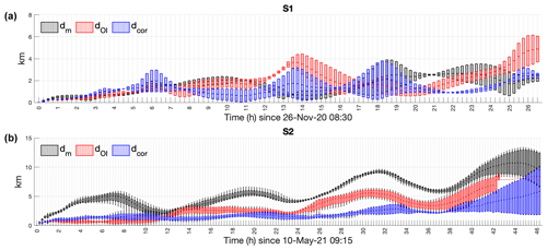
Figure 7 Boxplots of separation distance between the observed and reconstructed trajectories for drifters of S1 (a) and drifters S2 (b) using the initial and optimized model and the model after performing the wind-induced velocity correction. For S1 (a), where only two drifters are considered, the top and bottom edges of each box are the maximum and minimum values, and the line within the box indicates the median, equal to the mean. For S2 (b), the top and bottom edges of each box are the upper (0.75) and lower (0.25) quartiles, respectively. The line within the box indicates the median. The whiskers above and below each box are the nonoutlier maximum and minimum. During S2 (b), three of the four modeled trajectories escaped the domain around 42 h, resulting in a simple curve without boxplot.

On the whole, it is remarkable that the wind-induced velocity correction enables much better trajectory reconstruction during both S1 and S2. It allows a total reduction of d by 13 % during S1 and by 63 % during S2 (Table 1, columns 5–7). During S1, the optimization and correction processes produce realistic trajectories for both dinghies. During S1, the optimization and wind processes produce realistic trajectories, particularly for dinghies S2-1 and S2-3 (Fig. 8c, e). On the other hand, the corrected trajectories of S2-2 and S2-4 still lack precision compared to observed trajectories (Fig. 8d, f). At the time of deployment, S2-1 and S2-3 were to the south of the other pair, S2-2 and S2-4. It seems that the impact of the wind is different between these two pairs of buoys, even though they are only 1 km apart. This means that wind correction is less effective for drifters S2-2 and S2-4.

Compared to the separation distance d, the relative error ε (Table 1, columns 2–4) appears equal for both the optimized model and model after performing wind-induced velocity correction. Because the relative error accumulates over time, a small error does not imply the best trajectory reconstruction, either in space or time. This underlines the usefulness of separation distance for evaluating the model velocity field in terms of Lagrangian tracking.

Figure 8 Observed drifter trajectory (green lines) and the trajectory reconstructed after applying the wind-induced velocity correction (blue) for S1 (a, b) and S2 (c, d, e, f).

4.3 Absolute dispersion

After applying OI of velocity observations and correcting the wind-induced velocity, the resulting surface current fields are used with more confidence to assess dispersion processes, in particular by estimating the absolute dispersion. A total of 225 particles separated by 250 m were seeded within a rectangular shape area north of CGN. The center of mass of this cluster of particles, referred to hereafter as cluster-N, was located 1.7 km offshore. The second cluster, referred to as cluster-W, was located west of CGN with its center of mass separated from the shore by 2.1 km (Fig. 9a). Each cluster formed a rectangle of size 3.3 km by 3.5 km. The particles were advected during the 26 and 46 h time periods using the OceanParcels software. Three velocity fields were utilized: those provided by the initial model, the optimized model, and the model after applying the wind-induced velocity correction.

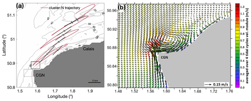
Figure 9 (a) Evolution of the spreading in cluster-N (6 h spacing) during S2. The red trajectory represents the trajectory of the center of mass of cluster-N particles. Semi-axes of the ellipse are represented by black lines. The length of semi-axis of the ellipse approximating the particle dispersion accounts for the particle spreading (A₁, A₂). Results were obtained with optimized surface currents after performing wind-induced velocity correction. The area of particle release is shown by a black rectangle for cluster-N and a grey rectangle for cluster-W. (b) Residual velocity around the CGN obtained by averaging the model velocities over four tidal cycles.

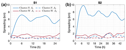
Absolute dispersion is used to quantify the rate of spreading. PCA allows the characterization of the dominant direction of spreading and the shape of a cluster of passively drifting particles at different time intervals. Figure 9a shows the time evolution of spreading along the ellipse axes (A₁ and A₂) during S2 at a 6 h time step roughly corresponding to the time of high and low water in Boulogne. The spreading appears significantly larger in the alongshore direction. Similar results are obtained for particles in cluster-W (not shown). The effect of tidal currents on particles spreading consists in elongation of the cloud of particles in the dominant current direction.

The time evolution of spreading during both surveys is shown in Fig. 10. Similar results are obtained during S1 and S2 with spreading that is estimated to be 4 times larger for cluster-N than for cluster-W (A₁=5.8 km for cluster-N and A₁=1.4 km for cluster-W during S1). Particles in cluster-N experienced very large spreading shortly after the release under stronger wind conditions observed during S2: A₁=10 km at time t=8 h (Fig. 10b). The spreading is found to be 30 % weaker (A₁=7 km) under northeastern wind conditions (S1) with lower wind speed (Fig. 10a). The enhanced spreading of particles in cluster-N is due to large velocity shear induced by an anticyclonic tidal eddy generated during flooding tide (Fig. 9b). Particles in this cluster are effectively driven by the eddy, whose higher nearshore velocities induce stirring of particles westward along the shore. When the tidal eddy weakens and disappears, A₁ slightly decreases, causing particle alignment in the main direction of the flow. At each peak flood tide, the stronger and heterogenous tidal flow coming from the Dover Strait towards the North Sea (mean velocity of 0.9 m s⁻¹ and spatial range of variation of 1.6 m s⁻¹) causes shear dispersion and increases the spreading rate. However, at each peak ebb flow, the spreading along the major axis decreases. Particles seem to become more concentrated when impacted by the weaker and homogenous tidal flow (mean velocity of 0.4 m s⁻¹ and spatial range of variation of 1.2 m s⁻¹). In contrast, particles in cluster-W are impacted only by the tip of the tidally induced eddy, pushing them toward the northeast, away from the area of high nearshore velocity. Thus, particles in cluster-W experience a relatively weak spreading during both survey periods (A₁<2.4 km).

In comparison to the model after interpolating the velocity measurements and performing the wind-induced velocity correction, the initial model tends to underestimate the spreading along the major axis A₁ by 20 %, whereas it tends to overestimate the spreading along the minor axis A₂ by 13 % for both clusters and both surveys. It should be mentioned that the optimized model and the model with wind-induced velocity correction provide nearly identical results (a 1 % difference is found).

Figure 10 Time evolution of spreading A₁ (solid line) and A₂ (dashed line) under environmental conditions observed during S1 (a) and S2 (b). Spreading of cluster-N is shown in blue and of cluster-W in dark red. Results are obtained from the model after performing a wind-induced velocity correction.

5 Discussion

The present study demonstrates how the Lagrangian observations can be used to improve the performance of the high-resolution model MARS. It is shown that the optimal interpolation of drifter data affects not only the model velocity fields but also the dispersion properties. Optimizing the model outputs and correcting for wind-induced velocity reduces the model–data misfit for velocity by 50 % and results in a significant (10 %–20 %) change of the dispersion rate caused by the correction of velocities.

Objective mapping methods, including OI, have been widely used in oceanographic studies. Sentchev and Yaremchuk (2015) and Thiébaut et al. (2019) applied the OI to constrain a high-resolution simulation of coastal currents by the MARS-2D model using towed acoustic Doppler current profiler (ADCP) measurements in the English Channel. They obtained a significant decrease of the model error (50 %), as the result of the velocity correction.

Kim et al. (2008) optimally interpolated the surface current velocities derived from high-frequency radar measurements along the west coast of the United States by using a predefined (exponential shape) isotropic spatial covariance function instead of a covariance matrix derived from ensemble model simulations. The method allowed one to obtain a continuous set of current vector maps by taking into account the measurement accuracy. A similar approach has been used for surface current mapping from satellite altimeter data at the global scale (e.g., Ma and Han, 2019; Wilkin et al., 2002).

The efficiency of optimal interpolation of drifter observations has been assessed in detail by Molcard et al. (2003). Using a quasi-geostrophic model within an idealized domain, an interpolation scheme based on general Bayesian theory, and twin data experiments with virtual drifters, the authors quantified the performance of data assimilation. For an optimal choice of parameters (number of drifters, sampling period, and uncertainties of observations and model outputs), the relative error between the observed and modeled quantities decreased from 58 % to 11 %. The final model–data discrepancy obtained in our study appears to be similar (Table 1, column 3). This increases confidence in the results of the proposed optimization technique.

In this study, we utilized fused data sources to assess fusion outcomes. Such an evaluation process may not objectively reflect the effectiveness of the fusion method and the characteristics of the real ocean current field. However, the “leave-one-out validation”, which uses one drifter trajectory as a control data set (repeatedly replaced) and other trajectories for optimization, provides a much less biased measure of error and enables trusting the fusion outcomes. An alternative to this technique, which requires more drifter trajectories, is the “cross-validation” method where high-resolution observational data could be partitioned into training and validation sets (Le Rest et al., 2013, 2014).

To further explore the performance of OI in application to drifter data in the tide-dominated basin, sensitivity of the model correction to the number of ensemble members was assessed. The results showed that in the EEC, the performance of OI was not significantly affected by the number of ensemble members. Increasing this number from 7 to 31 provided only a 10 % reduction in relative error. However, in regions with low tidal forcing (e.g., Mediterranean Sea) or with significant swell and freshwater inputs, selecting ensemble members could be more challenging. In such cases, alternative clustering methods like K-means clustering or SOMs (self-organizing maps) could be considered (Hernández-Carrasco et al., 2018; Nguyen-Duy et al., 2021; Solabarrieta et al., 2015).

A method of correction for the wind effect, often poorly represented in numerical models, especially during the periods of strong winds, appears simple, physically robust, and efficient. A comparison of the modeled and observed drifter trajectories revealed that wind-induced velocities are largely overestimated in M2D. As a result, a significant shoreward displacement of the modeled trajectory under strong southwestern winds was obtained (Fig. 6b). The mean separation distance between the observed and modeled trajectories attained 5 km (Table 1 column 5) and the maximum separation 13 km for drifter S2-3. In order to achieve better agreement, the wind-induced current velocity correction was done (Eq. 3) under the assumption of a stationary wind over the observation period. The wind time series from ARPEGE atmospheric model and observations at meteorological stations supported this choice. In principle, the method of correction can be easily adopted for situations with evolving wind. However, in other situations, for example, when the drifters were observed close to the shore (Fig. 6a), the correction method may be less efficient. In our case, the proposed correction method allowed the reduction of the separation distance between the observed and modeled trajectories by 63 % for S2, under strong winds, and by 13 % for S1, under weak winds (Table 1, column 7).

This highlights the importance of an accurate representation of the wind effect in high-resolution coastal circulation models. For example, the effect of the Stokes drift on passive tracers, drifting in the surface layer, should be accounted for. In fact, MARS is an Eulerian hydrodynamic model, not coupled with a wave model in the considered configuration. For this reason, wave–current interactions are neglected in the model. Moreover, the wave-induced current velocity (Stokes drift velocity), estimated as 1 % of the wind speed (Ardhuin et al., 2012, 2018), can considerably modify the transport pathways of passively advected particles. Dobler et al. (2019), van den Bremer and Breivik (2018), and Curcic et al. (2016) also highlighted the impact of the Stokes drift on the behavior of passive tracers, micro-plastics, and oil spills, especially under strong winds.

One of the practical applications of oceanographic studies is the assessment of turbulent dispersion of materials in the marine coastal environment. It attracts a growing interest because our seas and oceans are being degraded by human activities that harm marine life, undermine coastal communities, and inject harmful substances into the ocean (Landrigan et al., 2020). Marine turbulence is considered the main factor controlling the spreading of materials in seawater (van Sebille et al., 2020). The present study aims to evaluate the turbulent dispersion and demonstrate how the dispersion estimates can be improved in one of the busiest maritime straits. Optimal interpolation of drifter data was used to optimize the sea current velocities. It was found that the resulting change in the velocity field may lead to adjustment of the velocity gradients, which, in turn, increase the rate of dispersion. Consequently, the absolute dispersion in the model was found to be significantly larger after interpolation of the drifter data, which is not surprising given the results reported in other studies. Modeled velocities are generally lower and less variable than observed velocities (Kjellsson and Döös, 2012), especially under strong wind conditions (Curcic et al., 2016).

In addition, other studies highlighted that in tide-dominated regions, with large spatial variation of velocity, the coastal flow is characterized by strong shear dispersion (Van Dam et al., 1999; Zimmerman, 1986). In particular, an enhancement of the dispersion rate was found in the vicinity of headlands or under a significant bathymetric change (Geyer and Signell, 1992). Numerical studies in the English Channel have shown that passive particles released offshore experience lower dispersion compared to the particles released close to the shore where the bathymetry variation is large. Sentchev and Korotenko (2005) documented that under the joint effect of freshwater input and tides, a cluster of particles released in the nearshore coastal flow experienced large stretching along the shore. These results are in good agreement with the behavior of particles in cluster-N, affected by the near-shore coastal flow and tide-generated transient eddy.

6 Conclusions

In this study, we tested a computationally efficient method of combining numerical modeling with surface drifter observations to obtain a more reliable estimate of turbulent dispersion in the narrowest and most energetic part of the EEC: the Dover Strait.

Using optimal interpolation to combine the high-resolution MARS model outputs with two and four drifter trajectories allowed reconstruction of the surface velocity evolution with a 50 % reduction in the error between observed and modeled velocities. Additional correction of the wind-induced velocity component enabled the further reduction of the separation distance between observed and modeled trajectories (63 % reduction of separation distance under strong winds). Particle spreading, estimated from more realistic velocities, obtained after the OI and wind-induced current corrections, was found to be 20 % higher north of the CGN and 13 % lower south of the CGN, compared to the initial model run. Spatial variability in dispersion was identified. It is assumed to be related to small-scale features of the local circulation generated by tidal flow interaction with the headland (CGN) and irregular topography.

The proposed methodology can be used to improve existing decision-making support tools or to design new tools for monitoring the transport and dispersion of materials in coastal ocean environments.