Transport dynamics in a complex coastal archipelago

The Archipelago Sea (in the Baltic Sea) is characterised by thousands of islands of various sizes and steep gradients of the bottom topography. Together with the much deeper Åland Sea, the Archipelago Sea acts as a pathway to the water exchange between the neighbouring basins, Baltic proper and Bothnian Sea. We studied circulation and water transports in the Archipelago Sea using a new configuration of the NEMO 3D hydrodynamic model that covers the Åland Sea–Archipelago Sea region with a horizontal resolution of around 500 m. The results show that currents are steered by the geometry of the islands and straits and the bottom topography. Currents are highest and strongly aligned in the narrow channels in the northern part of the area, with the directions alternating between south and north. In more open areas, the currents are weaker with wider directional distribution. During our study period of 2013–2017, southward currents were more frequent in the surface layer. In the bottom layer, in areas deeper than 25 m, northward currents dominated in the southern part of the Archipelago Sea, while in the northern part southward and northward currents were more evenly represented. Due to the variation in current directions, both northward and southward transports occur. During our study period, the net transport in the upper 20 m layer was southward. Below 20 m depth, the net transport was southward at the northern edge and northward at the southern edge of the Archipelago Sea. There were seasonal and inter-annual variations in the transport volumes and directions in the upper layer. Southward transport was usually largest in spring and summer months, and northward transport was largest in autumn and winter months. The transport dynamics in the Archipelago Sea show different variabilities in the north and south. A single transect cannot describe water transport through the whole area in all cases. Further studies on the water exchange processes between the Baltic proper and the Bothnian Sea through the Archipelago Sea would benefit from using a two-way nested model set-up for the region.

1 Introduction

The Archipelago Sea is located in the Baltic Sea, between the Baltic Sea proper and the Gulf of Bothnia (Fig. 1), and together with the Åland Sea it acts as a pathway to the water exchange between these basins. The Archipelago Sea is characterised by a complex coastline bathymetry. There are over 40 000 islands and islets of various sizes. Though the mean depth is only about 19 m, there are deep fault lines crossing the area in N–S or NW–SE directions that are partly deeper than 100 m.

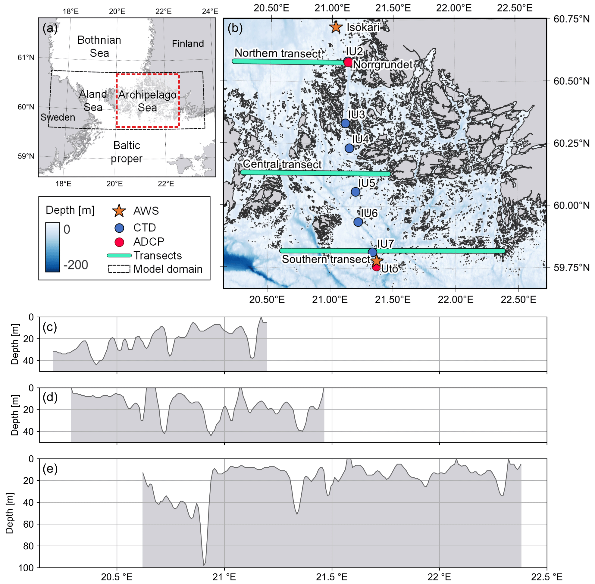
Figure 1 (a) Location of our study area, the Archipelago Sea, in the Baltic Sea (indicated with the dashed red line) and extent of the Åland Sea–Archipelago Sea model domain (indicated with dashed black line). (b) A more detailed map of the study area. Background colour represent the bathymetry (EMODnet Bathymetry Consortium, 2020). Orange stars indicate the locations of the automatic weather stations (AWSs), and blue and red dots indicate the locations of the hydrography (CTD, conductivity–temperature–depth) and current (ADCP, acoustic Doppler current profiler) measurements, respectively. Cyan lines indicate the locations of the transects used in volume transport calculations. Lower panels show the bottom topography in the model grid along the (c) northern, (d) central and (e) southern transects. (The coastline in panels (a) and (b) is drawn using data originating from OpenStreetMap and further processed by HELCOM (2018).)

A characteristic feature of the Archipelago Sea is that the currents, generated by winds and sea level differences, are strongly influenced by the geometry of the archipelago so that the channels crossing the area steer the currents and enhance their speed. There is a lot of spatial, seasonal and interannual variations in the current speeds. Deep channels intensify the strong currents generated by the high-wind events, strong surface tilt or their combination (Ambjörn and Gidhagen, 1979; Kanarik et al., 2018). The vertical extent of the strong currents is affected by the seasonal temperature stratification, which restricts the wind stress to the upper mixed layer. During summer the lower part of the water column can be stagnant.

In recent years, developments in hydrodynamic modelling have improved our capabilities to describe the dynamics of fragmented coastal regions that have, for example, an irregular coastline, numerous islands of various sizes, narrow straits, and/or steep bathymetry variations. Depending on the region, the required resolution and choice of methods (e.g., structured vs. unstructured grid) can vary a lot. The highest resolution (20–500 m) is needed in semi-enclosed basins, inlets and archipelagos (e.g., Aleynik et al., 2016; Khangaonkar et al., 2017; Murawski et al., 2021), whereas in more open coastal seas resolutions of a few kilometres may be sufficient (e.g., Liu et al., 2022; Mou et al., 2022).

The earlier studies on the circulation and transports in the Archipelago Sea region lacked observational and computational resources and were based on short time series of spatially sparse observations (Ambjörn and Gidhagen, 1979) or on models with insufficient resolution to describe the bathymetry variations and dense archipelago (e.g., Helminen et al., 1998; Myrberg and Andrejev, 2006). Our previous studies using a 3D hydrodynamic model with a resolution of approximately 500 m have highlighted the importance of grid resolution when describing the geometry of this area. For example, Tuomi et al. (2018) showed that earlier Baltic Sea models having a resolution of 3.7 km overestimated both the northward and southward transport of substances through the Archipelago Sea.

Both the southern and northern parts of the outer Archipelago Sea have constant exchange of water with their neighbouring basins, but most of the time the transports from Baltic proper and the Bothnian Sea (the southern part of the Gulf of Bothnia) only extend to the mid-part of the Archipelago Sea. Miettunen et al. (2020) showed that situations where substances are transported through the whole Archipelago Sea during a single event occur rarely. This suggests that the dense archipelago performs as a “buffer zone” where water masses are mixed.

Understanding the circulation dynamics of this area and the connections to the surrounding basins is vital to marine protection and management of this vulnerable area (HELCOM, 2013). The national monitoring network is focused on the inner parts of the Archipelago Sea, closer to the mainland, and there are gaps in both spatial and temporal data. Due to this, it is not possible to capture the dynamics of this heterogeneous area with the present monitoring network (e.g., Erkkilä and Kalliola, 2007; Nylén et al., 2021). Many studies on the water properties in the Archipelago Sea focus on specific seasons and locations or dedicated measurement campaigns (e.g., Suominen et al., 2010). These studies, however, do not use information on circulation, due to the unavailability of suitable measured or modelled data at the time. Satellites provide information on the surface layer with good spatial coverage, and they have been used to evaluate, for example, the variation in turbidity (e.g., Erkkilä and Kalliola, 2004). Recently, water quality model applications that utilise data from high-resolution hydrodynamic models have been developed for the Archipelago Sea to allow for a more comprehensive understanding of the system (Lignell et al., 2018; Vigouroux et al., 2019).

To enhance our understanding on the transports within and through the Archipelago Sea, we will use a new 3D hydrodynamic model configuration that is based on the NEMO model code (Nucleus for European Modelling of the Ocean; Madec and the NEMO System Team, 2019). It covers the Åland Sea–Archipelago Sea region with a resolution of approximately 500 m and has recently been used to study transport dynamics in the Åland Sea (Westerlund et al., 2022). We chose to update the earlier-used Archipelago Sea hydrodynamic model set-up (Tuomi et al., 2018; Miettunen et al., 2020) that was based on the COHERENS model code (Luyten, 2013) to NEMO to improve the description of stratification in the shallower areas. The change of model will also allow the use of the NEMO development work carried out by several institutions and consortia in the Baltic Sea (e.g., Hordoir et al., 2019; Westerlund et al., 2019; Kärnä et al., 2021).

This is the first time that a high-resolution hydrodynamic model configuration is used to estimate volume transports in the Archipelago Sea. To support the conclusions, we use hydrographic and current measurements to evaluate the adequacy of the model results in the Archipelago Sea. The inter-annual variation in the transport dynamics will be discussed, and the accuracy of the earlier estimates will be studied.

2 Material and methods

2.1 NEMO hydrodynamic model

We used the NEMO hydrodynamic model version 4.0.3 (Madec and the NEMO System Team, 2019) set-up for the Åland Sea and the Archipelago Sea (Westerlund et al., 2022). The NEMO model has previously been used in the Baltic Sea for several studies from regional (e.g., Hordoir et al., 2019; Kärnä et al., 2021) to basin scale (e.g., Vankevich et al., 2016; Westerlund et al., 2018, 2019).

The Åland Sea–Archipelago Sea model configuration has a horizontal resolution of 0.25 nautical miles (nmi) or approximately 500 m, and it covers the area between 59.60 to 60.75^∘ N and 17.32 to 23.58^∘ E (shown in Fig. 1a). In the vertical, the model uses the z^* coordinate system. There are 200 levels with a level thickness of roughly 1 m down to 120 m depth, below which the thickness more rapidly increases up to 8 m at the deepest parts of the model domain.

The bathymetry data for the model grid were compiled from two sources: VELMU (The Finnish Inventory Programme for Underwater Marine Diversity) bathymetry model (Finnish Environment Institute) for the Finnish EEZ (exclusive economic zone) and the Baltic Sea Bathymetry Database (Baltic Sea Hydrographic Commission) for the areas outside of the Finnish EEZ. The process of bathymetric data compilation and grid editing is described in Westerlund et al. (2022).

Meteorological forcing for the model (hourly 10 m winds, 2 m air temperature, 2 m dew point, mean sea level pressure, precipitation, snowfall rate, short-wave and long-wave radiation fluxes) was taken from the ERA5 atmospheric reanalysis (Copernicus Climate Change Service; Hersbach et al., 2018). Open boundary data at the northern and southern boundaries of the model domain were compiled from the Baltic Sea Physical Reanalysis Product (CMEMS, 2022), which had a horizontal resolution of 2 nmi. Sea surface heights were applied at the open boundary at 1 h intervals, and barotropic velocities, temperature and salinity were applied at 24 h intervals. Runoff data for the eight rivers that are inside the model domain were taken from the VEMALA watershed model (Huttunen et al., 2016).

The model simulation used in this study was the same as the one used in Westerlund et al. (2022), and it covered the period from June 2012 to the end of the year 2017. The first half a year was regarded as an initialisation period, and we analysed the results starting from the beginning of the year 2013. The modelled 3D fields of temperature, salinity and currents were saved as 6 h averages, and volume transports were saved once per day.

We calculated volume transports from the model results for three zonal transects (locations in Fig. 1). To calculate a time series, we integrated the volume transports over the whole transect: $F_{\mathrm{v}}=\iint v\mathrm{d}A=\iint v\mathrm{d}z\mathrm{d}l$, where v is the velocity across the transect, A is the area of the transect, z is the depth along the transect and l is the length of the transect. We also calculated the volume transport per unit length along the transect: ∫v dz.

2.2 Observational data

2.2.1 Hydrography

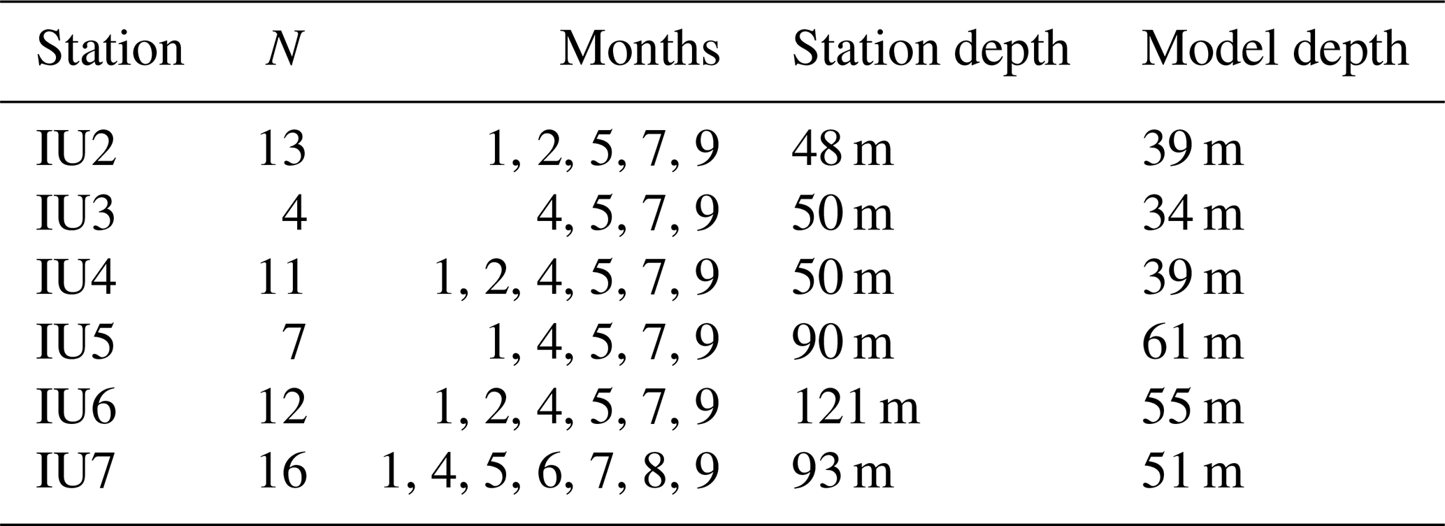
To validate the modelled temperature and salinity, we used data from the six most-visited monitoring stations in the Archipelago Sea. The stations are located along a transect directing through the outer archipelago from the northern to southern edge (locations shown in Fig. 1). In total, 4–16 profiles are available per station during our modelling period (Table 1). Measurements are mostly from winter, spring and late summer, and not all the stations have been visited annually. To compare the measurements with model data, we extracted the modelled temperature and salinity profiles from the nearest representative model grid point. The model grid points are 10–66 m shallower than the measurement stations. Measured salinity was converted from practical salinity to absolute salinity (g kg⁻¹) for the validation.

Table 1 Measurement stations used in model validation. N= the number of profiles from 2013–2017. Months = months that have at least one profile during these years.

2.2.2 Currents

We used current measurements from two locations from the Archipelago Sea, from which data were available during our modelling period. One of the locations is in the northern part of the Archipelago Sea in a narrow channel (hereafter called Norrgrundet) and the other is located in the southern edge of the Archipelago Sea near the Utö islands (hereafter called Utö). The measurements were carried out with Teledyne RD Instruments’ bottom-mounted 300 kHz Workhorse Sentinel broadband acoustic Doppler current profilers (ADCPs). At Norrgrundet, the bottom depth is 54 m (corresponding model grid point 39 m), and the measurements cover depths of 5 to 49 m and the period of 6 September 2016 to 16 October 2018. At Utö, the bottom depth is 76 m (corresponding model grid point 55 m), and the measurements cover depths of 7 to 71 m and the period of 26 July 2017 to 27 June 2018. In both datasets, vertical resolution is 1 m and time interval is 30 min. Locations of the measurement sites are shown in Fig. 1.

2.2.3 Wind speed and direction

As wind is one of the most important forces inducing currents in the Archipelago Sea, we also validated the ERA5 winds against two automated weather stations (AWSs), namely Utö and Isokari (locations shown in Fig. 1). The Utö AWS is located in Utö island at the southern edge of the Archipelago Sea and represents open sea wind conditions from the SW–SE sector. Isokari island is at the northern edge of the Archipelago Sea and does not fully represent open sea conditions, but it gives better estimates for high winds from the W–NE sectors than the Utö AWS.

3 Model validation

Westerlund et al. (2022) validated the modelled sea surface height by comparing the model results (saved at 1 h intervals) with the observed sea level at Föglö Degerby station. This station is located in the western Archipelago Sea (at 60.03^∘ N, 20.38^∘ E), and it is the only tide gauge inside the model domain that was considered representative of the overall sea level variation in the area. The comparison showed that the model was able to reproduce the sea level variations and their timing quite well. Westerlund et al. (2022) also presented validation of hydrography and currents in the Åland Sea part of the model domain. Here, we show validation of these variables for the Archipelago Sea part.

To validate temperature and salinity, we compared the model results with measurements from six stations. We divided the water column into layers of 10 m and calculated the bias and RMSE for each of these layers. As the temperature and salinity profiles are sampled at 1 m intervals, the number of measurements in each layer is up to 10 times the number of profiles from which these depths were available. Down to 40 m depth, measurement data were available from all six stations, and below that data were only available from the three southernmost stations (IU5, IU6 and IU7).

Similar to the results shown in our earlier study (Westerlund et al., 2022), there is a bias in the salinity, with too low modelled salinities in the upper 30 m and too high in the lower layer below 40 m (Table 2). We believe this is at least partly caused by the bias in the boundary condition. Due to these biases, the haline stratification in the model is too strong. Of the six validation stations, halocline is seen only at IU7, and there is seasonal variation in its occurrence and depth (also shown by Laakso et al., 2018). IU7 is located at the southern edge of the archipelago and represents more the open sea conditions than the Archipelago Sea. The model grid around the location of this station is too shallow to reproduce the halocline. However, this has no effect on the main analysis of this study, as the majority of the Archipelago Sea, north from IU7 station, has no halocline.

Table 2 Comparison of modelled salinity and temperature against measurements from the CTD stations (locations are shown in Fig. 1). N= the number of observations in each depth range.

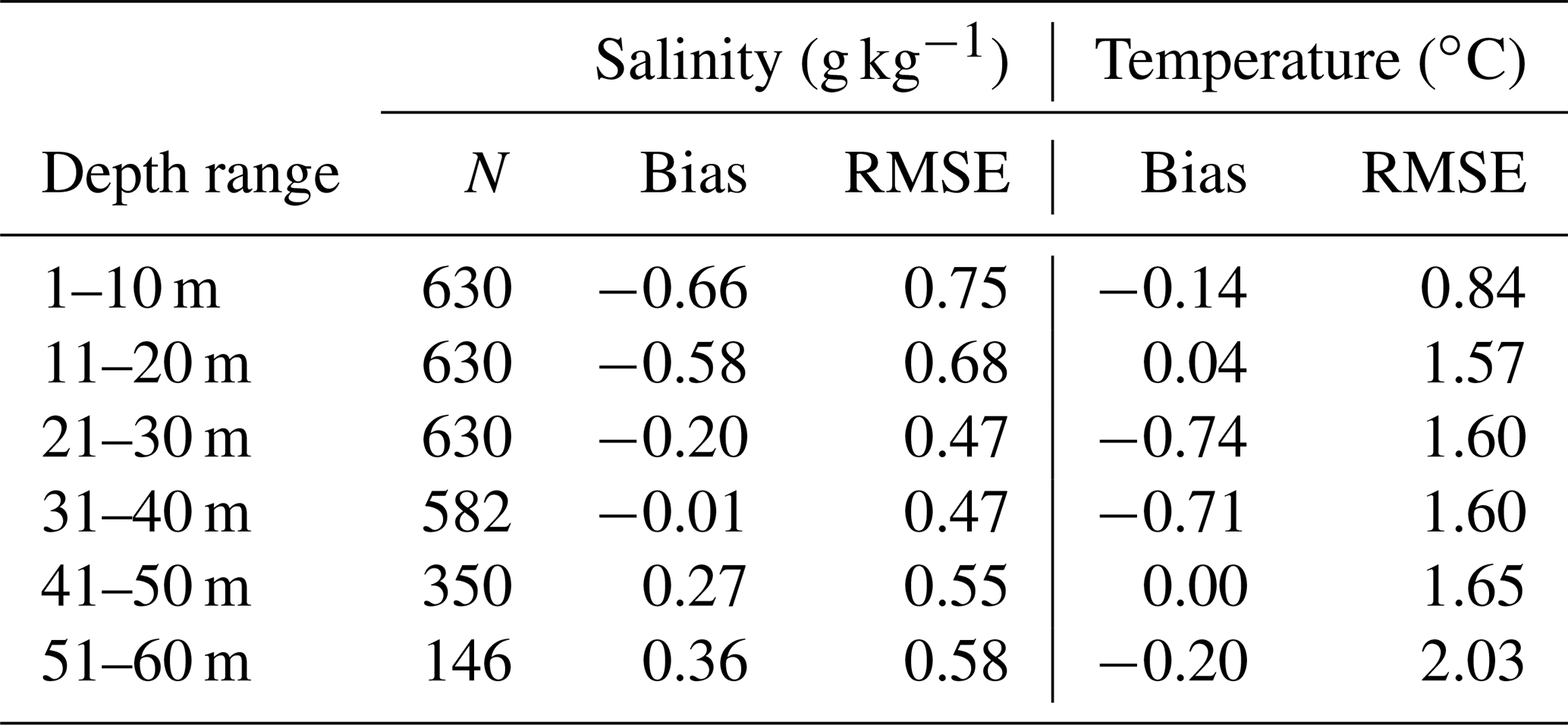
In modelled temperature, there was a slight underestimation at the 10 m surface layer and at the depths of 51–60 m (Table 2). The bias was largest at the depths of 21–40 m, up to −0.74 ^∘C. RMSE increased with depth, being smallest at the surface layer and largest at 50–60 m depths. The modelled seasonal thermocline was well represented.

To validate the currents, we compared the model results with measurements from two ADCPs. Direction distribution of the modelled currents is slightly narrower than that of measured currents both in Norrgrundet and Utö (Fig. 2). This is partly due to the inability of the regular model grid to represent narrow channels that are not entirely oriented in N–S or E–W directions.

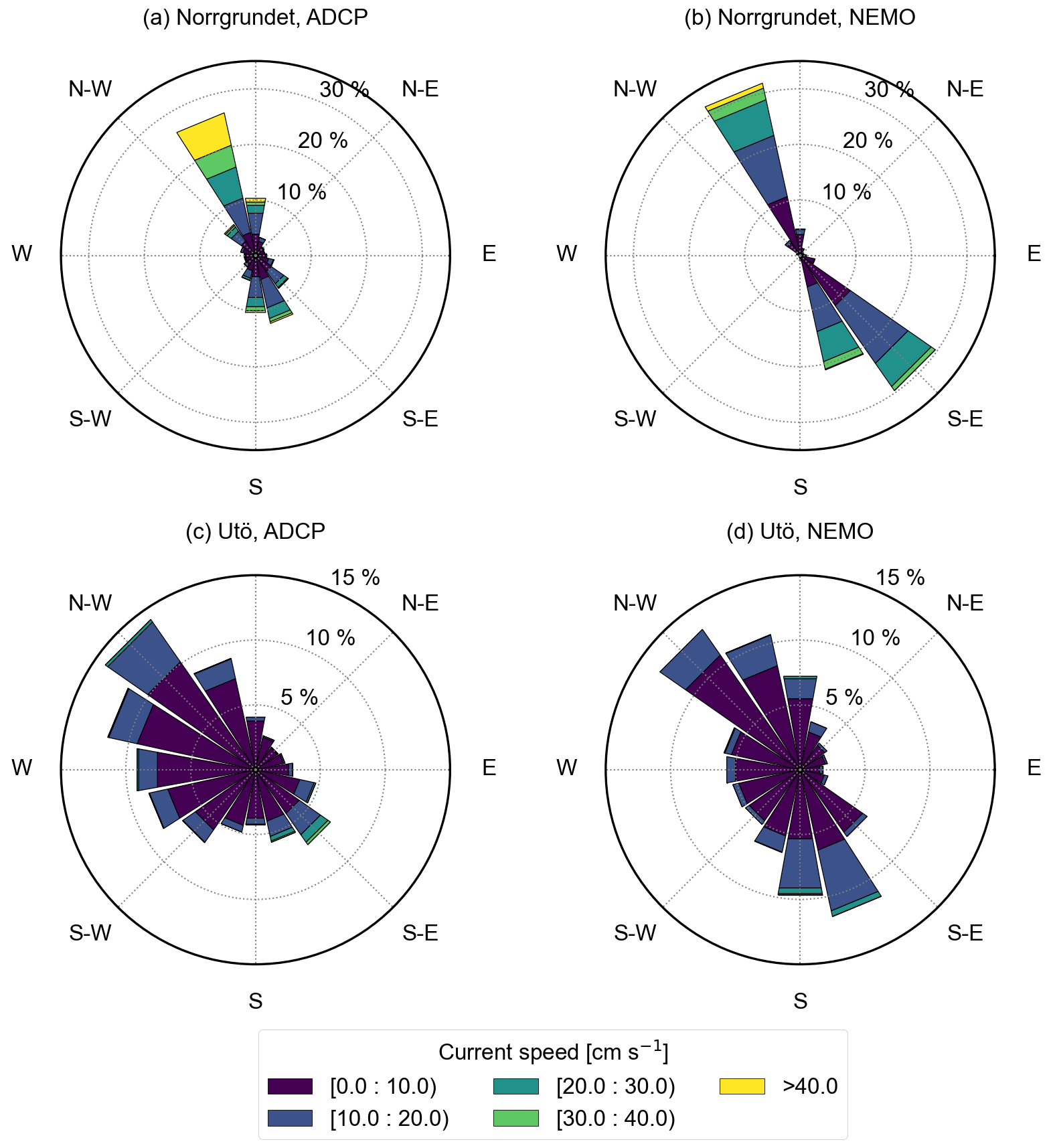
Figure 2 Current roses (direction to) drawn from the measured (ADCP) and modelled currents at Norrgrundet in 6 September 2016–31 December 2017 (a, b) and at Utö in 26 July 2017–31 December 2017 (c, d). The topmost and bottommost 5 m are excluded from the model data, as they are also missing from the ADCP data.

In Norrgrundet, the measured currents are strongly oriented toward NNW or SSE because the measurement station is located at the mouth of a narrow channel leading toward the archipelago. The model shows a similar direction distribution but does not catch all the highest current events, with current speed of over 50 cm s⁻¹. Comparison shows negative bias in speed for the whole water column, being highest, −11 cm s⁻¹, in the bottommost layer. These underestimations can partly be addressed to the used wind forcing, which underestimates the frequency and speed of high winds (shown in Fig. 3). The modelled currents also show too low frequency of northward currents, which could be related to ERA5 showing a lower frequency of winds from S/SSE and E sectors than measurements.

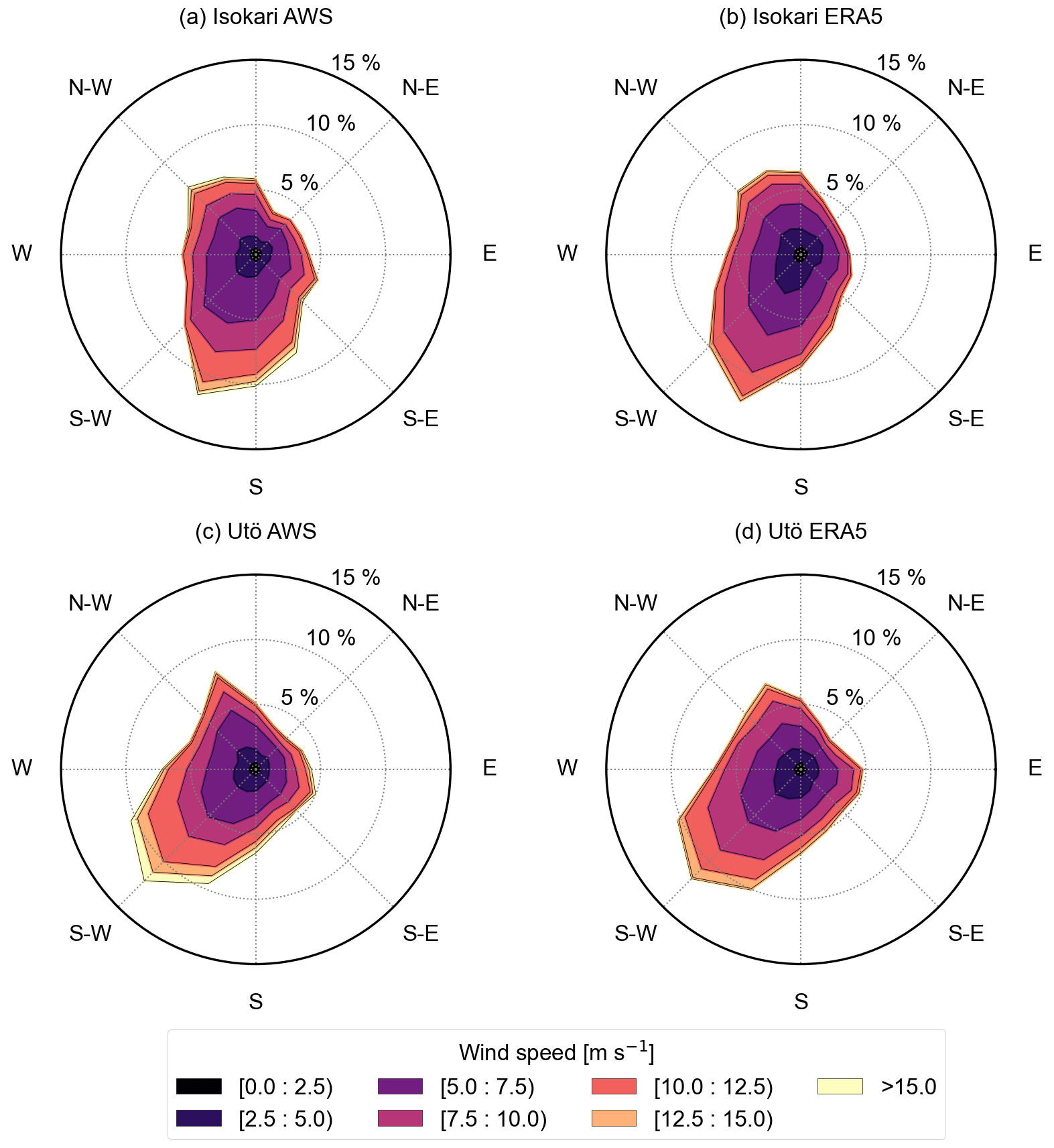
Figure 3 Wind roses (direction from) for years 2013–2017 drawn from Isokari (a) and Utö (c) AWS data compared to wind roses drawn from the ERA5 forcing data at the corresponding grid point (b, d).

In Utö, the model slightly underestimated the current speed in the upper 25 m (bias up to −1 cm s⁻¹), with the largest bias occurring at around 10 m depth. At the depths of 25–42 m, the model overestimated the current speed (up to 2 cm s⁻¹), and the largest bias occurred around 37 m depth. Below 42 m depth, the bias was again negative, and the largest underestimation was at the bottom layer with the bias being −5 cm s⁻¹. The RMSE of the current speed varied between 4–6 cm s⁻¹, and largest values occurred in the surface and bottom layers as well at the depth of 37 m.

Both in Norrgrundet and Utö, the bias in modelled current speed is largest at the bottommost layer. That is because the measurement points are deeper than the corresponding model grid points, so the modelled current is already slowed down by the bottom friction at depths where the measured current does not feel the bottom yet.

4 Currents in the Archipelago Sea

The modelled currents show how the geometry of the islands and straits and bathymetry affect the circulation. The openness of sub-basins considerably impacts the directional distribution of the currents. In the northern part of the Archipelago Sea, the currents are strongly aligned along the N–S-oriented channels, and the current directions in the 5 m surface layer alternate between north and south (Fig. 4). Current speeds are also strongest in these narrow channels, and high current speeds exceeding 40 cm s⁻¹ occur frequently in the easternmost channel in the north as well as the westernmost channels south of 60.15^∘ N. In the more open parts in the central and southern outer archipelago, currents are weaker and have a wider directional distribution, but the most frequent directions are southeast and northwest. The southward and south-eastward current directions mostly dominate throughout the model domain. An exception is the easternmost channel in the north, in which there are almost as much northward current components as southward components.

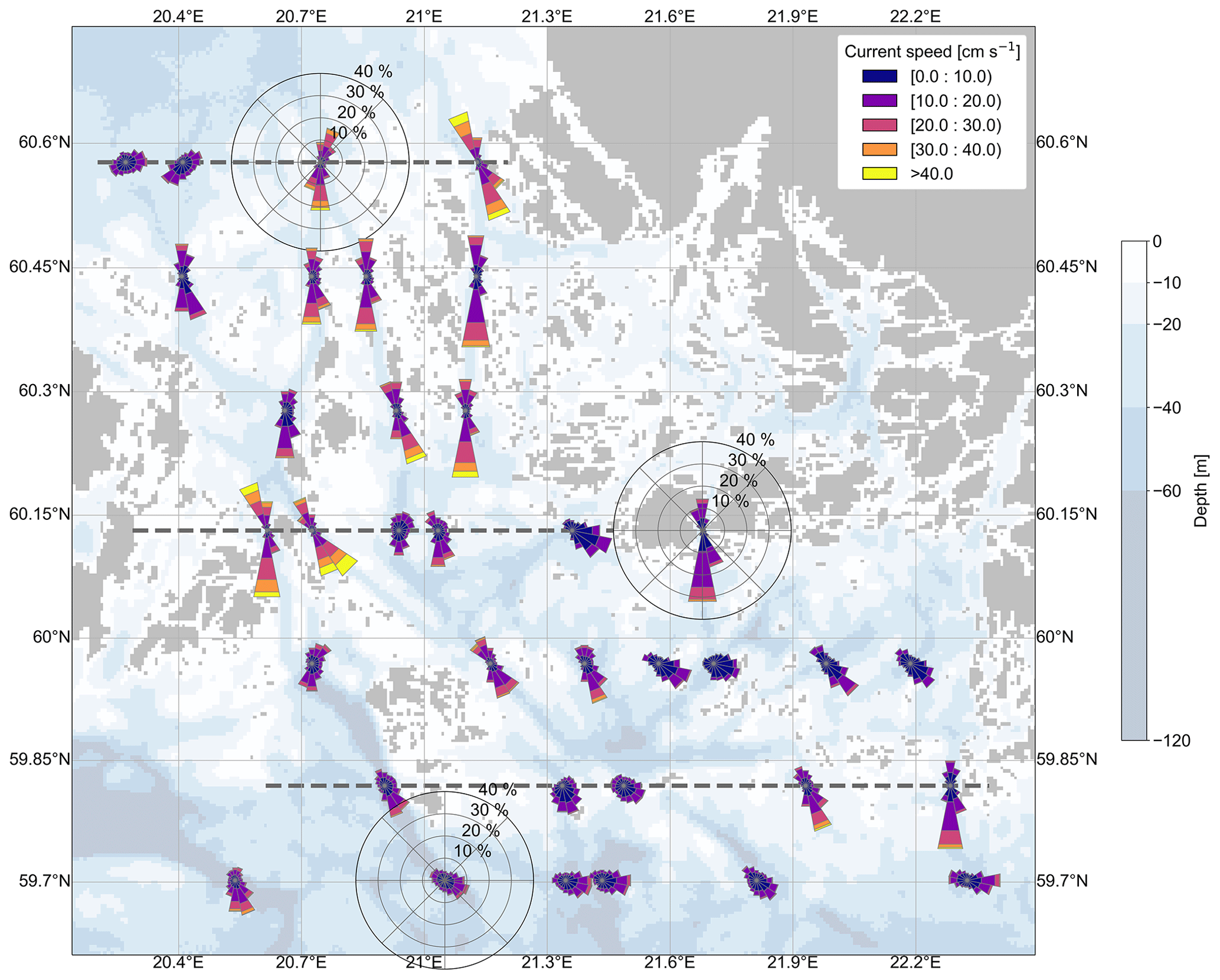
Figure 4 Modelled currents (direction to) in selected model grid points in the uppermost 5 m layer, 2013–2017. Each current rose shows the distribution of direction and magnitude of currents in the grid point at the centre of the rose. All current roses have the same axis limits, and for clarity the axes are drawn only for three of them. Dashed grey lines indicate the locations of the transects used in the volume transport calculations.

In areas deeper than 25 m, the directional distribution of currents in the bottommost 5 m layer (Fig. 5) is strongly aligned by the bathymetry also in the southern part of the area. The northward currents dominate in the bottom layer in the southern part of the Archipelago Sea, whereas in the northern part southward and northward currents are as common. Generally, the current speed is less than 10 cm s⁻¹ in the bottom layer. Currents above 10 cm s⁻¹ are seen in the narrow channels and even above 20 cm s⁻¹ in the easternmost channel in the north and in the channel northeast from Utö.

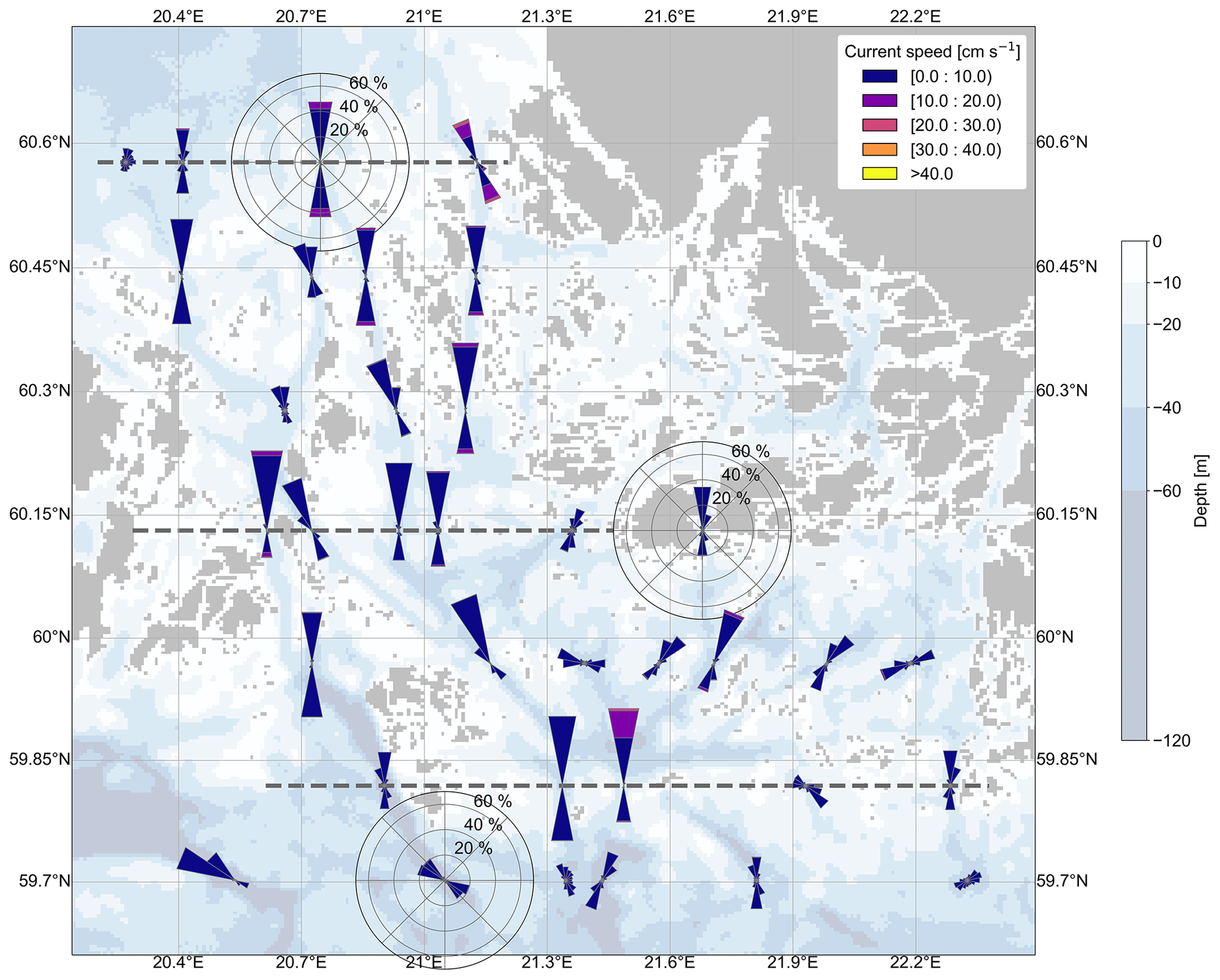
Figure 5 Modelled currents (direction to) in selected model grid points in the bottommost 5 m layer, 2013–2017. Each current rose shows the distribution of direction and magnitude of currents in the grid point at the centre of the rose. All current roses have the same axis limits, and for clarity the axes are drawn only for three of them. Dashed grey lines indicate the locations of the transects used in the volume transport calculations.

As wind is one of the main drivers of the surface currents in the Archipelago Sea, the interannual variability in currents is strongly connected to the one in the wind conditions. During our modelling period, years 2013 and 2015–2017 resemble the long-term mean more than year 2014, which shows larger percentage of winds from eastern and south-eastern sectors compared to the long-term mean (Fig. 6). Also, winds from the west-southwestern sector are almost completely missing in 2014. Because of the geometry of the archipelago and the orientation of the channels, winds from the south-eastern sector in particular are able to induce strong northward currents in the Archipelago Sea (Kanarik et al., 2018). Therefore, the main features of the circulation are different in 2014 than in the other years, as already demonstrated by Tuomi et al. (2018). It should be noted that due to the bi-directional nature of the currents, mean values do not reflect the circulation in the Archipelago Sea.

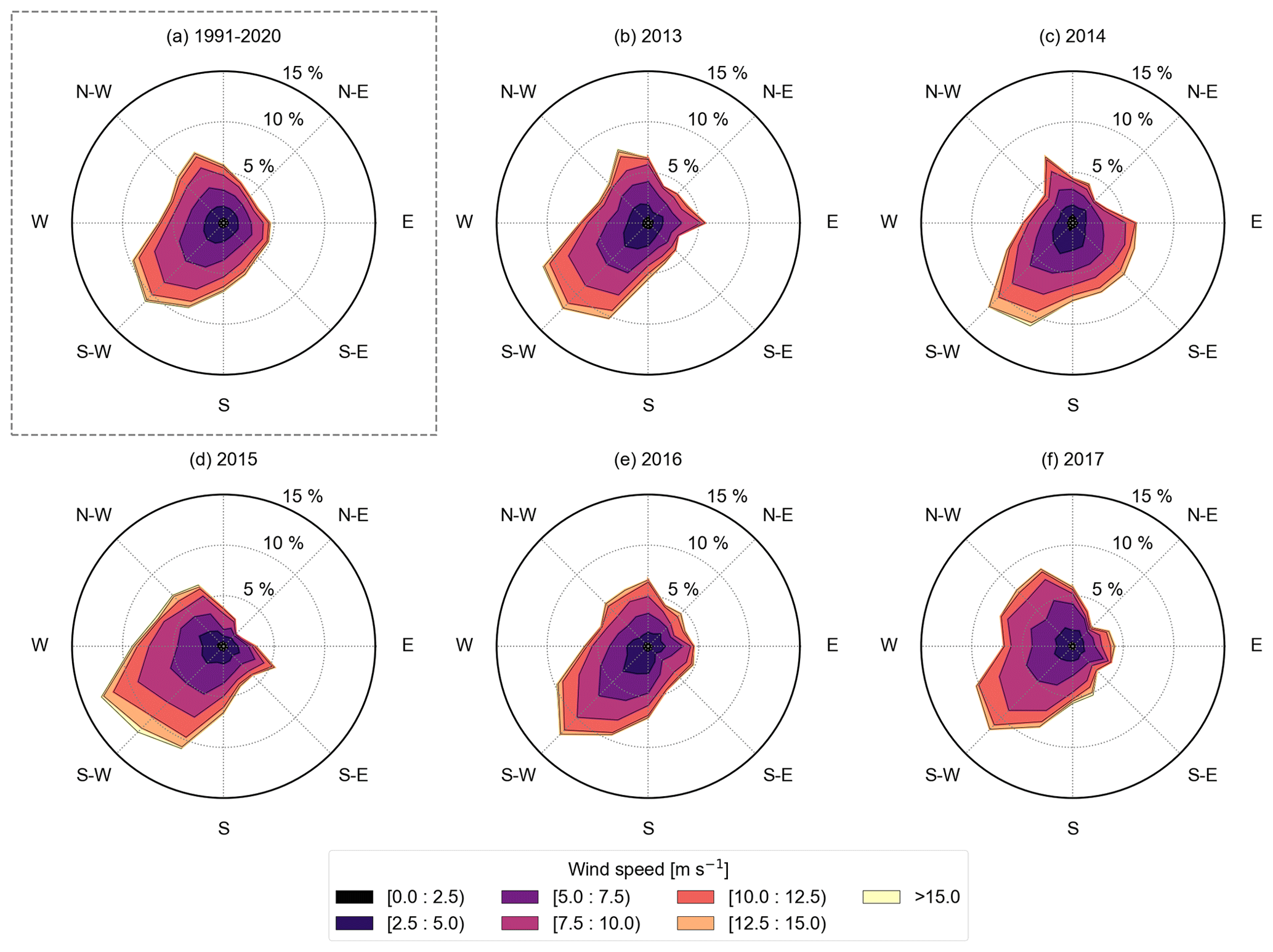
Figure 6 Wind roses from the ERA5 forcing data in the grid point corresponding the location of Utö AWS for the 30-year period of 1991–2020 (a) and for the years 2013–2017 (b–f).

5 Volume transport in the Archipelago Sea

To study volumes and different routes of water transport in the Archipelago Sea, we analysed modelled volume transports along three zonal (west–east) transects across the area. The northern and southern transects are located approximately at 60.58^∘ N and 59.82^∘ N, and they represent transports entering or leaving the Archipelago Sea at its northern and southern edges, respectively. The central transect is located at 60.13^∘ N, chosen to get an estimate of transports within the area. Bottom topography along the transects is shown in Fig. 1.

Transports were integrated over the whole water column but also separately for the surface layer above 20 m depth (representing the mixed layer above the seasonal thermocline) and the lower layer below 20 m depth. As the Archipelago Sea is generally shallow and the channels that are deeper than 20 m are quite narrow, the transport in the upper layer dominates the transport integrated over the whole water column. The shallow areas of the central Archipelago Sea also limit the lower layer transport through the area.

First, we calculated monthly volume transports from the time series integrated along the transects separately for the upper and lower layers. In addition to the monthly net transport, we also calculated the northward and southward components separately to show the effect of the bi-directional currents in the area.

The monthly net volume transport integrated along the whole transect is mainly southward in the upper 20 m layer at all three transects (Fig. 7). Transports in the lower layer below 20 m, on the other hand, are different in the north and south (Fig. 8). At the northern transect, the monthly net transport in the lower layer is mainly southward, while at the southern transect it is mainly northward. Compared to the northern parts of the Archipelago Sea, the volume transport in the lower layer is larger in the southern part, as a larger portion of the transect is deeper than 20 m (Fig. 1). At the central transect, northward transports dominate in the lower layer, but the values are really small as the bottom layer current speeds are low, correspondingly (Fig. 5).

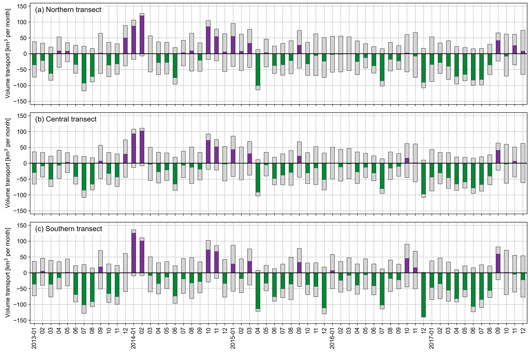
Figure 7 Monthly transport (km³ per month) in the upper layer in the northern (a), central (b) and southern (c) Archipelago Sea. Grey bars indicate the northward (positive) and southward (negative) monthly transport separately, and the purple and green bars indicate the net transport.

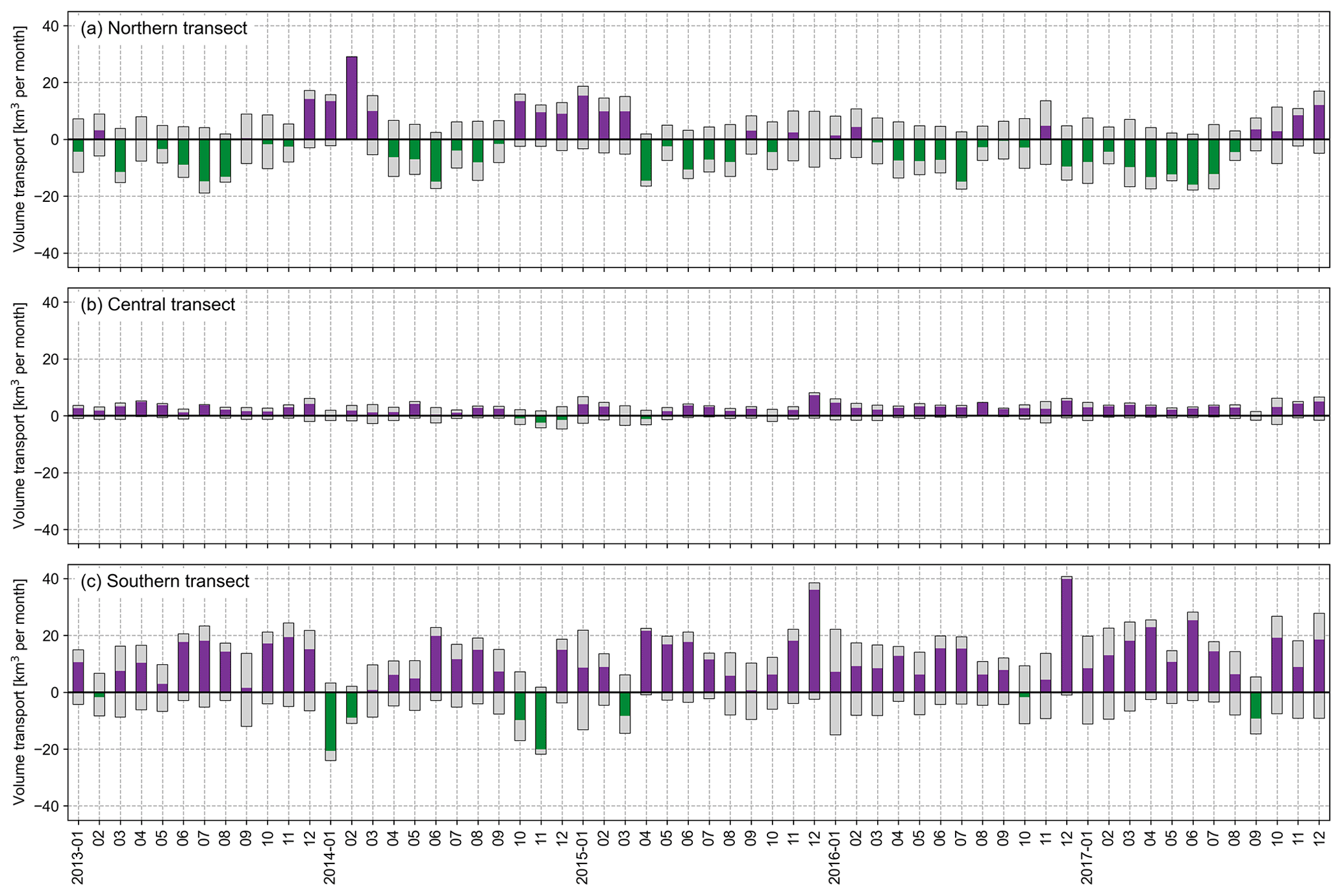
Figure 8 Monthly transport (km³ per month) in the lower layer in the northern (a), central (b) and southern (c) Archipelago Sea. Grey bars indicate the northward (positive) and southward (negative) monthly transport separately, and the purple and green bars indicate the net transport. Note the different y axis limits compared to Fig. 7.

Although the net transport is southward in the surface layer, there is seasonal and annual variation in the direction and volume of the transport. Southward transport was typically largest during spring and summer. Northward transport in the surface layer was most common in autumn. An exception was the year 2014, which differs from the long-term mean in wind conditions (Sect. 4) and, consequently, also in circulation and transport (Tuomi et al., 2018; Westerlund et al., 2022). Then northward transport was dominant in winter and autumn months and was of the same order of magnitude as southward transport in the other 4 years we studied. In some months with very small net transport, typically occurring in autumn or winter, there are actually quite large northward and southward components balancing each other (grey bars in Figs. 7 and 8).

The monthly variation in the transport volumes and directions in the surface layer is similar at all three transects (Fig. 7). However, there are periods when the net transport is toward opposite directions in the north and south. In the lower layer, the direction of the net transport at the northern transect show similar variation than in the upper layer. At the southern transect, on the other hand, the transport direction in the lower layer is generally opposite to that in the surface layer.

To get an overview of directions and volumes as well as their inter-annual variability along the three transects, we calculated yearly volume transports per unit length in each model grid point along the three transects for each simulation year (not shown). In the upper 20 m layer, the yearly net transport in 2013 and 2015–2017 was mainly southward at all three transects. In the lower layer below 20 m, the net transport was mainly southward at the northern transect but northward at the central and southern transects. In 2014, the net transport was mainly northward both in the upper and lower layers at all transects, but there were some channels where the net transport was southward, especially the channel east of Utö island at the southern transect and near the western edge of the northern transect. The largest transports were seen in the narrow channels of the northern Archipelago Sea where the currents are strongest and the current direction alternates between north and south.

As the Bothnian Sea has water exchange both with the Archipelago Sea and the Åland Sea, it is interesting to compare the transports at the northern edge of the Archipelago Sea with our earlier transport estimates at the northern Åland Sea (Westerlund et al., 2022). To compare, we chose one additional transect in the northern part of the Åland Sea, located at 60.3^∘ N. This transect was also used in Westerlund et al. (2022), in which it is named “Märket South”, and it represents the transport entering to or leaving from the Åland Sea at its northern boundary.

The monthly net transports integrated over the whole water column are generally larger in the northern Åland Sea than in the northern Archipelago Sea, as the Åland Sea is much deeper (Fig. 9). The temporal variation in transport direction is generally similar in both transects. However, there are months when these two regions show different dynamics so that while the net transport at the northern Archipelago Sea transect is close to zero, the net transport at the Åland Sea transect is clearly northward (October 2016) or southward (e.g., August 2014, January–February 2016 and October 2017).

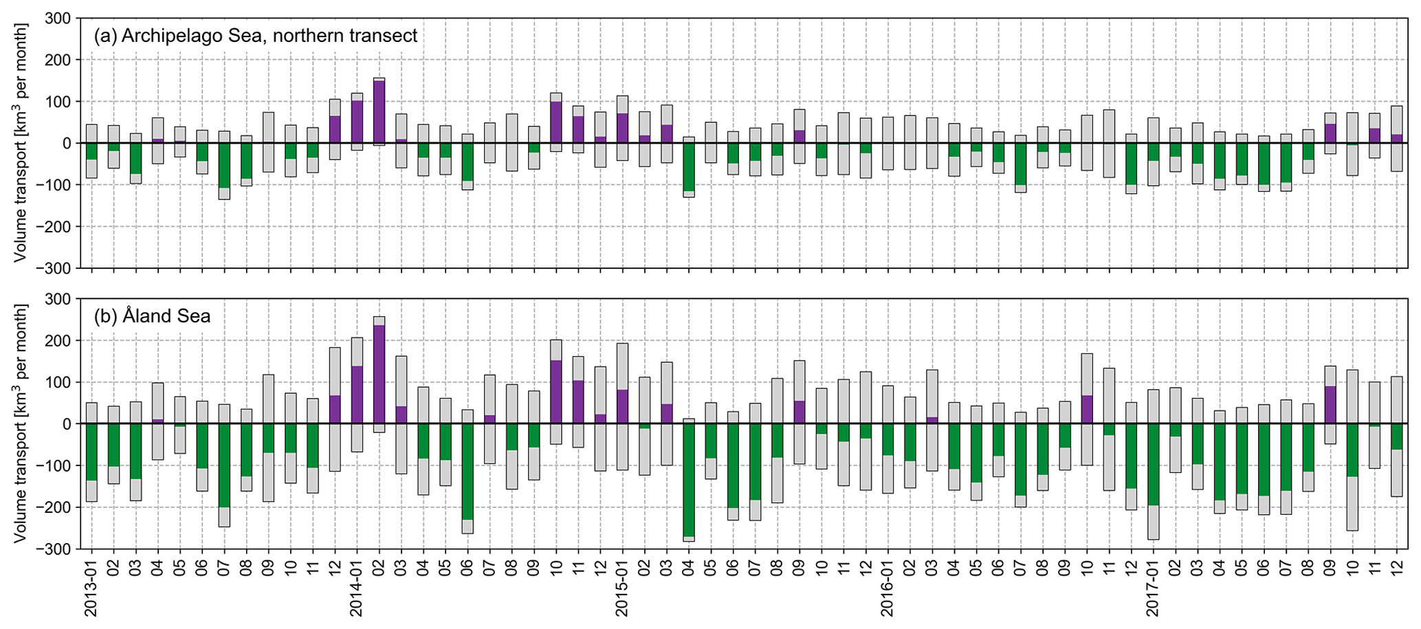
Figure 9 Monthly transport (km³ per month) in the whole water column in the northern Archipelago Sea (a) and the northern Åland Sea (b). Grey bars indicate the northward (positive) and southward (negative) monthly transport separately, and the purple and green bars indicate the net transport. Note the different y axis limits compared to Figs. 7 and 8.

Averaging over our study period of 2013–2017, the mean of the net transport over the northern Archipelago Sea transect is −206 km³ per year. This is approximately 28 % of the mean net transport over the Åland Sea transect which was −745 km³ per year. While the net transports in the Åland Sea are generally larger than in the Archipelago Sea, in the year 2014 the net northward transport at the northern edge of the Archipelago Sea was 1.3 times larger than at the northern edge of the Åland Sea. If the year 2014 were left out when averaging, there would be less cases of northward transport and the resulting mean net transport would be −321 km³ per year at the northern Archipelago Sea transect and −979 km³ per year at the Åland Sea transect.

6 Discussion

Our results show that the net transport in the surface mixed layer is southward during the study period. This is expected due to the voluminous river discharges to the Gulf of Bothnia flowing out of the gulf through the Åland Sea and the Archipelago Sea. The earlier estimates of transports have suggested the opposite, that is, northward net transport through the Archipelago Sea (Ambjörn and Gidhagen, 1979; Helminen et al., 1998). However, there are months with northward net transport also during our study period (especially during winters 2013–2014 and 2014–2015).

Ambjörn and Gidhagen (1979) estimated the monthly volume transports through the Åland Sea and the Archipelago Sea in June–August 1977 based on current measurements in five locations in the northern Åland Sea and three locations in the Archipelago Sea (Table 3). For June, the estimated net transports were small and directed southward in both areas, whereas for July and August the net transport was southward in the Åland Sea and northward in the Archipelago Sea.

Table 3 Monthly volume transports (in km³ per month) from Ambjörn and Gidhagen (1979).

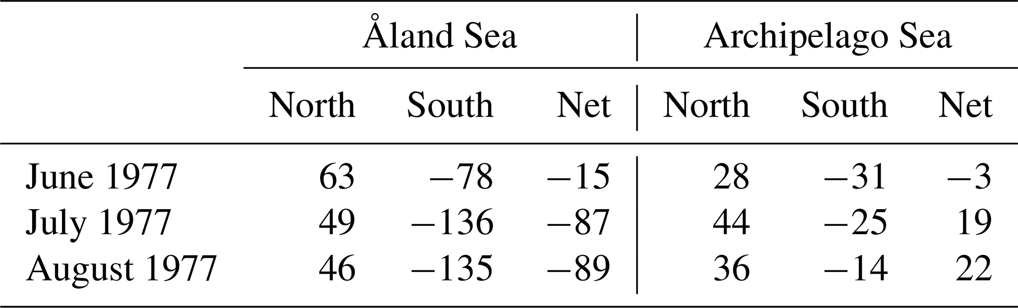
Compared to their estimates, the orders of magnitude of our modelled monthly net transports are similar in both areas. However, their estimate suggests northward net transport in the Archipelago Sea, whereas our model shows southward net transport. The transport estimate for the Archipelago Sea by Ambjörn and Gidhagen (1979) is based on short measurement time series limited to thermally stratified season in 1977. Compared to the long-term wind conditions in Utö AWS, the most frequent directions during this period were NNW, S and E, and the SW winds typical for the area were mostly missing. Thus, their transport estimates represent a specific summer season and are not representative for the long-term annual mean conditions in the area.

When studying transports in an area like the Archipelago Sea, the locations of the transects must be chosen carefully so that they represent what they are intended to. The estimates of Ambjörn and Gidhagen (1979), for the Archipelago Sea, are based on measurements at three locations, chosen to represent the three deepest and largest channels crossing the area. As one is located at the northern edge of the area and two in the central part of the area, they represent different parts of the archipelago. Given the complexity of the archipelago and the differences in the modelled current direction distribution between the different parts of the area, it is not straightforward to find a single transect to describe transport through the whole Archipelago Sea from the Baltic proper to the Bothnian Sea or vice versa. Though the upper layer transports in our study are mainly southward at all transects, there are periods when the transport direction is opposite in the north and south. In the lower layer, the transport directions at the northern and southern transects are almost all the time the opposite, while the net transport volumes at the central transect are really small. Based on our earlier studies, the transport through the whole area rarely occurs during a single event but requires 1–2 months on average (Miettunen et al., 2020). This indicates that the water masses transported from the Baltic proper from the south and the Bothnian Sea from the north mix in the mid-part of the Archipelago Sea. A more detailed study is required to estimate the residence times of water parcels and mixing of water masses in this region.

Our simulation period, 5 years, is relatively short. However, with the high-resolution model set-up the computational cost is heavy and this makes long hindcasts a challenge. As the surface currents are mainly wind-driven, the interannual variation in currents and transports is related to the interannual variation in wind conditions. To generalise our results, we compared the wind conditions during these 5 years against the long-term mean wind conditions. During the years with winds that resemble the long-term wind conditions with dominant SW winds, the net transport in the Archipelago Sea is southward. However, exceptions occur, like the year 2014 that had a larger contribution of SE and NNW winds than on average and showed northward net transport. Seasonal variation in transports is also related to the wind conditions but also to the freshwater discharge to the Gulf of Bothnia. The river discharges are largest in spring (Leppäranta and Myrberg, 2009), and southward net transport is usually strongest in spring and summer, when the winds are usually weaker. In autumn and early winter, the winds are stronger, there are fewer northerly winds than in spring or summer, and the volume of northward transport is largest. To capture these interannual and seasonal variations in transport directions, several years have to be modelled. Although longer periods would reduce the uncertainties in the transport estimates, we consider our modelling period to be a good representation of the overall dynamics in this area.

Modelling in archipelago areas like the Archipelago Sea is challenging because of the patchiness of the archipelago and the steep bathymetry variations. As shown in our earlier studies (Tuomi et al., 2018; Miettunen et al., 2020), modelling in this area requires sufficiently good bathymetric data but also a resolution high enough to describe the bathymetry in sufficient detail. High-resolution model data in this study enable us to gain a more comprehensive understanding of circulation and transport dynamics in this area than the earlier estimates presented, for example, by Ambjörn and Gidhagen (1979) and Helminen et al. (1998).

Compared to the earlier COHERENS-based configuration that used the σ coordinates in the vertical (Tuomi et al., 2018; Miettunen et al., 2020), this new NEMO-based configuration uses the z^* vertical coordinate system and, as a result, has less vertical mixing and produces stronger clines. Thus, it describes the seasonal stratification more accurately. This also improves the description of the circulation during the seasonal stratification, which was demonstrated by the possibility to evaluate the model results against recent current measurements. However, uncertainties remain regarding, for example, the bathymetric data (Westerlund et al., 2022), the grid resolution (Tuomi et al., 2018), and the accuracy of both the lateral boundary conditions and the atmospheric forcing data. Because the reanalysis data used as the open sea boundary conditions are daily averages, except the sea surface height that have the temporal resolution of 1 h, phenomena with smaller timescales than 1 d cannot be fully accounted for. Also, the biases in the open boundary data can easily affect large parts of the model domain. As noted already by Westerlund et al. (2022), one way to address the issues caused by the boundary conditions would be to develop a two-way nested configuration with the Åland Sea–Archipelago Sea model used in this study and a coarse resolution Baltic Sea model.

With a two-way nested model set-up, the dynamics of this buffer zone between the Baltic proper and the Gulf of Bothnia could be studied more comprehensively. It could also be used to study dynamics that affect the state of the Bothnian Sea: for example, at which depths and along which route can nutrient-rich water flow to the Bothnian Sea and when does this kind of water transport occur. Further, we could study if there have been changes in the water exchange dynamics which would in part explain the changes that have been recently observed in the state of the Bothnian Sea (e.g., Kuosa et al., 2017; Polyakov et al., 2022). We could also study the exchange between the Archipelago Sea and the Baltic proper and the Bothnian Sea and how these open sea areas affect the coastal waters, e.g. in the terms of nutrient loads.

7 Conclusions

This is the first time that transports in the Archipelago Sea and between the Archipelago Sea and the Bothnian Sea have been studied using a high-resolution coastal modelling system. The 5-year simulation period and good spatial coverage allow a detailed evaluation of the circulation and transport dynamics.

Our analysis showed that the currents generated by winds and sea level differences are steered by the geometry of the islands and straits and the bottom topography. In the narrow channels, current directions alternated between south and north in the northern part of the Archipelago Sea and between south-east and north-west in the southern part. More open areas in the southern part of Archipelago Sea showed a wider directional distribution of currents. In the surface layer, southward and south-eastward currents were slightly more frequent. In the bottom layer in the areas deeper than 25 m, northward currents dominated in the southern part of the area, whereas in the northern part southward and northward currents were more evenly represented.

Due to the bi-directional currents, both northward and southward water transports occur in the Archipelago Sea. The southward flow is more frequent in the surface layer, though in suitable wind conditions water flow from south to north through the whole area is possible. This is partly due to the voluminous freshwater discharge to the Gulf of Bothnia leading to southward net volume transport in the 20 m upper layer. Southward transport is usually largest in spring and summer months. Northward transport is largest in autumn and winter months. In the lower layer, below 20 m depth, the net transport is southward in the northern part of the Archipelago Sea and northward in the southern part.

The net volume transports in the Archipelago Sea are smaller than in the Åland Sea because the former is much shallower. During our simulation period, the mean yearly net transport at the northern edge of the Archipelago Sea is approximately one-third of that at the northern edge of the Åland Sea. At times, the transport dynamics in the Archipelago Sea show different variability than in the Åland Sea. For example, there are months when the direction of the net transport is close to zero at the northern edge of Archipelago Sea, while at the northern edge of the Åland Sea the net transport is clearly northward or southward. In general, however, the monthly variation in the direction of the net transports is similar in both areas.

The transport dynamics in the Archipelago Sea show different variabilities in the north and south so that a single transect cannot represent the transport through the whole area in all cases. More comprehensive studies on the role of the Archipelago Sea in the water exchange processes between the Baltic proper and the Bothnian Sea are needed and would benefit from using a two-way nested model set-up with the high-resolution Åland Sea–Archipelago Sea model and a coarser-resolution Baltic Sea model.