Investigating extreme marine summers in the Mediterranean Sea

The Mediterranean Sea (MS) has undergone significant surface warming, particularly pronounced during summers and associated with devastating impacts on marine life. Alongside the ongoing research on warming trends and marine heatwaves (MHWs), here we address the importance of understanding anomalously warm conditions also on the seasonal timescale. We propose the concept of extreme marine summers (EMSs) and investigate their characteristics in the MS, using sea surface temperature (SST) reanalysis data spanning 1950–2020. We define EMSs at a particular location, as the summers with a mean summer SST exceeding the 95th percentile. A marine summer may become extreme, under various SST substructures. Results show that, in most of the basin, EMSs are formed primarily due to the warmer summer days being warmer than normal. Areas where the warmest (coldest) part of the SST distribution is more variable experience EMSs primarily due to the warmest (coldest) part of the distribution being anomalously warm. MHWs occurring within EMSs are more intense, longer lasting, and more frequent than usual mainly in the northern MS regions. These enhanced MHW conditions occur mainly within the warmest part of the SST distribution. By means of temporal coverage of MHW conditions, a more pronounced occurrence of MHWs in EMSs is found for the central and eastern basin where up to 55 % of MHW days over 1950–2020 fall within EMSs. The role of air–sea heat fluxes in driving EMSs is quantified through a newly proposed metric. Results suggest that surface fluxes primarily drive EMSs in the northern half of the MS, while oceanic processes play a major role in southern regions. Upper-ocean preconditioning also contributes to the formation of EMSs. Finally, a detrended dataset was produced to examine how the SST multi-decadal variability affects the studied EMS features. Despite leading to warmer EMSs basin-wide, the multi-decadal signal does not significantly affect the dominant SST substructures during EMSs. Results also highlight the fundamental role of latent heat flux in modulating the surface heat budget during EMSs, regardless of the long-term trends.

1 Introduction

The global ocean has been experiencing intensive warming over the past decades (Bulgin et al., 2020; EU Copernicus Marine Service Product, 2022a). Being the interface between ocean and atmosphere, the sea surface temperature (SST) is a fundamental climate variable and global climate change indicator. A rapidly growing literature has shown its key role in the intensification of atmospheric/oceanic events and processes, e.g. heavy precipitation events (Pastor et al., 2015), surface air temperature variations (Xu et al., 2020), marine heatwaves under global warming (Frölicher et al., 2018), and increase in global wave power (Kaur et al., 2021). More importantly, SST is the oceanic parameter that regulates the air–sea energy exchanges, reflecting the role of the ocean's thermal inertia in the global climate (Deser et al., 2010).

The Mediterranean Sea (MS) is considered one of the most responsive and vulnerable areas to global warming (Giorgi, 2006; Lionello et al., 2006; Ali et al., 2022). In fact, the Mediterranean SST warming trends over the past decades largely exceed the observed global sea surface warming. Based on satellite SST recordings over the period 1982–2018, Pisano et al. (2020) report a trend of 0.041 ± 0.006 °C yr⁻¹ for the Mediterranean SST. Over shorter time periods, Shaltout and Omstedt (2014) and Mohamed et al. (2019) based on satellite SST observations compute a mean warming trend for the MS of 0.035 ± 0.007 °C yr⁻¹ (1982–2012) and 0.036 ± 0.003 °C yr⁻¹ (1993–2017), respectively. Consistently, the Ocean Monitoring Indicator (OMI) produced in the framework of the Copernicus Marine Environment Monitoring Service (CMEMS) provides a rate of Mediterranean SST change over the period 1993–2021 of 0.035 ± 0.002 °C yr⁻¹ (EU Copernicus Marine Service Product, 2022b). On top of the documented SST trends, future climate projections suggest additional warming in the basin until the end of the 21st century (Adloff et al., 2015; Alexander et al., 2018; Soto-Navarro et al., 2020). The high-emission scenarios (SSP5-8.5) of the CMIP6 multi-model projections suggest an SST increase of 0.8 to 3.5 °C in near-term (2021–2040) and long-term (2081–2100) 21st century, respectively, relative to 1995–2014 (Iturbide et al., 2021).

The well-documented warming over the instrumental period spanning 1980–present is also part of the significant multi-decadal variability of the Mediterranean SST. Marullo et al. (2011) first evidenced an approximately 70-year period SST oscillation in the basin in coherence with the North Atlantic Oscillation (NAO) and Atlantic Multi-decadal Oscillation (AMO). Several studies followed, suggesting different mechanisms regulating the observed multi-decadal SST fluctuations in the basin. Mariotti and Dell'Aquila (2012) attributed the transmission of AMO variability to the MS to atmospheric processes, while Skliris et al. (2012) suggested an oceanic origin of the AMO signal transmission in the basin. The source of the Mediterranean SST multi-decadal variability is still an open question. Pisano et al. (2020) showed that the linear increase of the Mediterranean SST observed over the satellite era closely follows AMO only until 2007. By that time, AMO has entered a declining phase, in agreement with the observed upper-ocean cooling in the Atlantic that reversed the previous warming trends in the Atlantic (Robson et al., 2016). Regarding the origin of the SST multi-decadal variability in the MS, Yan and Tang (2021) showed a better consistency of SST anomalies with a time-integrated NAO index, suggesting the accumulative effect of NAO atmospheric forcing on ocean circulation in the basin.

Along with the surface warming, extreme warm oceanic events such as marine heatwaves (MHWs) have attracted great research interest. MHWs are discrete events lasting at least 5 consecutive days, with temperatures exceeding a percentile-based (90 %) threshold (Hobday et al., 2016). Over the past decades, an increased MHW intensity and frequency have been documented based on observational and modelled SST datasets (Darmaraki et al., 2019a; Juza et al., 2022; Pastor and Khodayar, 2023; Dayan et al., 2023). Further increase of MHW trends is expected in the basin over the 21st century due to anthropogenic forcing and especially under high-emission scenarios (Darmaraki et al., 2019b; Oliver et al., 2019; Plecha and Soares, 2019).

Summer periods in the MS are of particular interest as they are associated with greater surface warming trends over the past decades, compared to other seasons (Giorgi and Lionello, 2008; López García and Camarasa Belmonte, 2011; Gualdi et al., 2013; Pastor et al., 2020; Pisano et al., 2020). Model projections further highlight summers, as the season expected to exhibit the maximum surface warming magnitudes (Giorgi and Lionello, 2008; Shaltout and Omstedt, 2014), as well as a significant increase (decrease) of extremely high (low) SSTs (Alexander et al., 2018).

The elevated summer SST holds significant implications for marine life in the MS. Several studies have already disclosed the detrimental impacts of thermal stress on marine ecosystems in the MS mainly during summer months, as “warm range edge” species are the most vulnerable to high SST anomalies (Smale et al., 2019). Either gradual warming or acute thermal stress (e.g. during a MHW) can greatly threaten marine ecosystems through direct (e.g. mortality events, decreased abundance of marine species) or indirect (e.g. nutrient availability, biodiversity) effects (Smale, 2020, and references therein). For instance, documented consequences include mass mortalities, massive geographical shifts, altered primary productivity, coral reef degradation, diminished fertilization success of certain species, and habitat loss in the MS (Perez et al., 2000; Coma et al., 2009; Garrabou et al., 2009; Marbà and Duarte, 2010; Kersting et al., 2013; Pearce and Feng, 2013; Rivetti et al., 2014; Smale et al., 2019; Gómez-Gras et al., 2021; Garrabou et al., 2022; Smith et al., 2023). Such findings point out the need to better understand the stressful conditions experienced by marine ecosystems due to abnormally high summer SSTs in the basin, caused either by short-lasting heat anomalies or elevated temperatures persisting for longer periods.

Alongside the ongoing research on long-term warming trends and warm ocean extreme events in the MS, here we address the importance of understanding anomalously warm conditions in the basin also on the seasonal timescale. Marine organisms have different ways to adapt to thermal stress depending on their sensitivity (thermal tolerance) and the duration and intensity of temperature anomalies. For example, they are more susceptible to increased summer temperatures if they live in regions close to their thermal limits (e.g. Smale et al., 2019). Investigating statistical properties of entire extremely warm summers across the basin is, therefore, highly relevant to impacts on different marine species.

In this context, we propose the concept of extreme marine summer (EMS). We define an EMS at a particular location as the summer presenting a mean marine summer (July–August–September) SST above the 95th percentile of mean summer values within 1950–2020 of this location. Considering the 71 summers within the study period, we identify the four EMSs that exceed this threshold at each location (see Methods) in order to explore their characteristics in relation to summer climatological conditions. EMSs are expected to be related to warm events, as the abnormally high mean summer SST of an EMS may emerge from a MHW occurrence within this summer, yet fundamental differences exist. MHWs typically last for days and may reach several weeks according to their causing factors and the concurrent atmospheric and oceanic conditions regulating their duration. On the other hand, an extreme marine season is, by definition, of fixed duration. Moreover, a marine summer may present extreme mean conditions under various SST substructures during the season, i.e. due to different parts of the SST distribution being anomalously warm, or due to a uniform shift of the SST distribution, potentially in absence of extreme SST values or extreme warm events.

Changes in SST generally result from the interplay of atmospheric and oceanic factors, being the air–sea heat exchanges (turbulent and radiative fluxes) and horizontal (Ekman and geostrophic currents) and vertical (entrainment, Ekman pumping) advection (Deser et al., 2010, and standard oceanography references therein). As the crucial role of the air–sea heat fluxes in the Mediterranean SST variability and observed warming trends in particular has been shown in several studies (e.g. Skliris et al., 2012; Shaltout and Omstedt, 2014), an extra focus is put within this study on understanding what is the driving role of the air–sea heat fluxes in the formation of EMSs. The upper-ocean thermal conditions before the beginning of the summer season, potentially favouring the development of an EMS, are additionally examined by means of a proposed preconditioning index.

Aim of this study is to explore the Mediterranean EMSs within 1950–2020, focusing on four objectives. The first is to understand how daily SST values are commonly structured within EMSs within the basin. Our second objective is to investigate the co-occurrence of MHWs during EMSs. The third is to investigate physical mechanisms related to the EMS formation focusing on the driving role of air–sea heat fluxes while briefly examining additional factors, such as wind speed, mixed layer depth, and preconditioning. Finally, the fourth objective is to understand how the Mediterranean SST multi-decadal variability affects the observed EMS characteristics.

The paper's content is organized as follows: Sect. 2 presents the datasets and methods used in the study. Section 3 discusses results on the SST substructures of EMSs (Sect. 3.1), the occurrence of MHWs within EMSs (Sect. 3.2), and potential EMS drivers focusing on air–sea heat fluxes (Sect. 3.3). The role of the Mediterranean SST multi-decadal variability is discussed throughout the different sub-sections. Finally, Sect. 4 summarizes key findings and conclusions.

2 Data and methods

2.1 Datasets

In this study, we use SST fields from the ERA5 Reanalysis of the European Centre for Medium-Range Weather Forecasts (ECMWF) for the period 1950–2020 (Bell et al., 2020; Hersbach et al., 2023). This reanalysis dataset corresponds to foundation SST (SST free of diurnal variations) and includes a combination of the HadISST2 and OSTIA datasets. Atmospheric variables from the ERA5 product are also used to investigate their role in the formation of EMSs: 10 m wind speed, net short-wave and long-wave radiation at the sea surface, latent and sensible surface heat fluxes, total cloud cover, and specific humidity. All fields have a grid spacing of 0.25° × 0.25° in longitude and latitude and are provided in hourly time intervals. To cross-check the quality of the reference dataset (ERA5) against a high-resolution observational SST dataset, we also use the CMEMS L4 satellite SST product (EU Copernicus Marine Service Product, 2022c) for the period 1982–2019, at 0.05° × 0.05° spatial resolution. Finally, mean monthly values for the mixed layer depth (MLD) and the ocean temperature are extracted from the CMEMS Physics Reanalysis product (EU Copernicus Marine Service Product, 2022d) for the period 1987–2019 at 0.042° × 0.042° spatial resolution, in order to compute the ocean heat content (OHC). The CMEMS MLD is additionally used to examine stratification conditions during EMSs.

2.2 Methods

2.2.1 Extreme marine summer definition and associated SST substructures

We consider July–August–September (JAS) as the marine summer season, i.e. the warmest part of the SST annual cycle in the MS (Pastor et al., 2020). We then identify EMSs within 1950–2020, separately at each grid point, on the basis of mean summer values. In particular, we define EMSs at each grid point as the summers presenting mean JAS SST above the 95th percentile of the mean summer SST values within 1950–2020 for the respective grid point. Considering the 71 summers of the study period, there are 4 summers exceeding this percentile threshold at each location. We considered the 95th percentile as a good compromise between the “extremity” of EMSs and a sufficient number of EMSs to be analysed per grid point, given the temporal length of the study period. The detection of EMSs (and consequent analysis) is performed per grid point. This approach captures periods with a low probability of occurrence experienced locally, allowing for a statistical analysis of their properties in a consistent way across the basin, based on the methodology of Röthlisberger et al. (2020). In this way we investigate separately each grid point with regards to the substructures of its own distribution of SSTs. To offer the reader an understanding on the EMS detection output regarding the spatial extent of the most significant EMS years, Fig. B1 in Appendix B illustrates the spatial extent of EMSs concentrating at least 50 % of the MS grid points (2015, 2003, 2018, and 2012, covering 72 %, 58 %, 54 %, and 53 % of the basin, respectively).

The observed surface warming trend across the basin during the last decades directly impacts the detection of EMSs, which tend to fall within the last few decades, especially in the post-2000 period. To study EMSs independently of long-term changes, we create an additional SST dataset, free of multi-decadal variability (henceforth referred to as detrended). The detrended dataset is used in addition to the actual SST time series (henceforth referred to as original dataset). For detrending the time series, we follow the methodology described in Sect. 2.2.2.

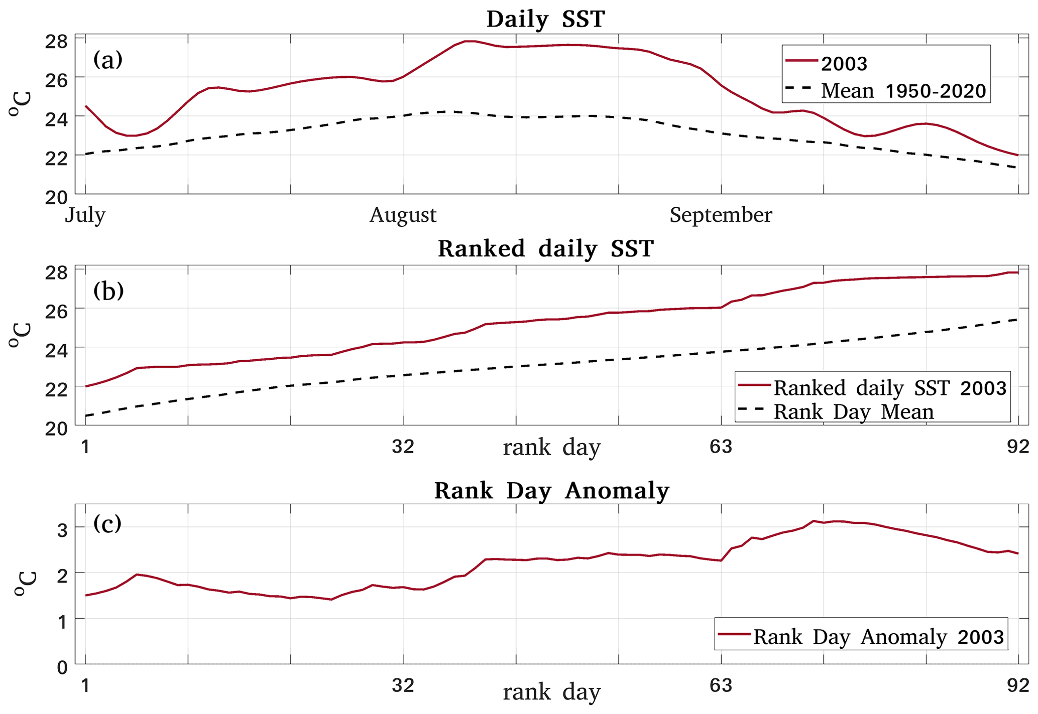
Figure 1 (a) Daily SST time series at a grid point in the Ligurian Sea (42.5° N–8° E) for the extreme marine summer 2003 and for the mean 1950–2020 state (solid red and dashed line, respectively). (b) Ranked daily SST values of (a) for 2003 and rank day means for 1950–2020 (solid red and dashed line, respectively). (c) Anomaly of each ranked daily SST with respect to the corresponding rank day mean value for 1950–2020. There is no temporal order in the horizontal axes of (b) and (c).

After identifying EMSs (using either the original or the detrended SST dataset), we apply the methods of Röthlisberger et al. (2020) to assess the associated SST substructures at each grid point. We first rank the 92 daily SST values within each summer (lowest daily SST, second-lowest daily SST, and so on) as shown in the illustrative example of Fig. 1. Then, we compute the anomaly of each ranked daily SST (referred to as rank day anomaly – RDA from now on) of the identified EMSs with respect to the ranked daily climatological mean SST value (Fig. 1c). This is done by subtracting the climatological mean SST of a rank day d (rank day mean) from the SST of that rank day d belonging to the examined EMS (SST_d,EMS), as follows:

$$\begin{array}{}\text{(1)}& {\mathrm{RDA}}_{d,\mathrm{EMS}}={\mathrm{SST}}_{d,\mathrm{EMS}}-{\displaystyle \frac{\mathrm{1}}{\mathrm{71}}}\sum _{s=\mathrm{1}}^{\mathrm{71}}{\mathrm{SST}}_{d,s},\end{array}$$

where RDA_d,EMS is the rank day anomaly of rank day d of the extreme summer EMS.

We then compute the mean SST anomaly of the four locally identified EMSs with respect to climatology, as follows:

$$\begin{array}{}\text{(2)}& \begin{array}{rl}\mathrm{MA}& ={\displaystyle \frac{\mathrm{1}}{\mathrm{4}}}\sum _{\mathrm{EMS}=\mathrm{1}}^{\mathrm{4}}{\displaystyle \frac{\mathrm{1}}{\mathrm{92}}}\sum _{d=\mathrm{1}}^{\mathrm{92}}{\mathrm{SST}}_{d,\mathrm{EMS}}\\ & -{\displaystyle \frac{\mathrm{1}}{\mathrm{71}}}\sum _{s=\mathrm{1}}^{\mathrm{71}}{\displaystyle \frac{\mathrm{1}}{\mathrm{92}}}\sum _{d=\mathrm{1}}^{\mathrm{92}}{\mathrm{SST}}_{d,s}.\end{array}\end{array}$$

Then, we divide the distribution of rank day anomalies computed in Eq. (1) into two equal parts: the coldest and the warmest half, ranging from the 1st to the 46th rank day and from the 47th to the 92nd rank day, respectively. In this way, we can quantify the relative contribution from each of the two parts of the distribution to the mean EMS anomaly (MA), based on the equations:

$$\begin{array}{}\text{(3)}& {\displaystyle }{\mathrm{Contr}}_{\mathrm{coldest}}=\left({\displaystyle \frac{\mathrm{1}}{\mathrm{4}}}\sum _{\mathrm{EMS}=\mathrm{1}}^{\mathrm{4}}{\displaystyle \frac{\mathrm{1}}{\mathrm{92}}}\sum _{d=\mathrm{1}}^{\mathrm{46}}{\mathrm{RDA}}_{d,\mathrm{EMS}}\right)/\mathrm{MA}\text{(4)}& {\displaystyle }{\mathrm{Contr}}_{\mathrm{warmest}}=\left({\displaystyle \frac{\mathrm{1}}{\mathrm{4}}}\sum _{\mathrm{EMS}=\mathrm{1}}^{\mathrm{4}}{\displaystyle \frac{\mathrm{1}}{\mathrm{92}}}\sum _{d=\mathrm{47}}^{\mathrm{92}}{\mathrm{RDA}}_{d,\mathrm{EMS}}\right)/\mathrm{MA}.\end{array}$$

As a result, we can diagnose whether EMSs are primarily formed due to the highest rank (i.e. warmest) days or to the lowest rank (i.e. coldest) days, being anomalously warm. The example of Fig. 1a shows for a certain grid point, and for a single EMS (2003) of this grid point, that this summer has been entirely warmer than usual. However, RDAs in this example (Fig. 1c) are larger for the warmest half of the RDA distribution compared to the coldest half. This shows that this summer has become extreme, in terms of mean summer SST, with a greater contribution of the warmer summer days being warmer than usual.

Finally, we examine the role of the local rank day SST variability in forming the observed SST substructures of EMSs. To do so, we first compute the variance (Var) of all RDA_d,s values for all 71 summers, at each grid point:

$$\begin{array}{}\text{(5)}& \mathrm{Var}={\displaystyle \frac{\mathrm{1}}{\mathrm{71}}}\sum _{s=\mathrm{1}}^{\mathrm{71}}{\displaystyle \frac{\mathrm{1}}{\mathrm{92}}}\sum _{d=\mathrm{1}}^{\mathrm{92}}({\mathrm{RDA}}_{d,s}{)}^{\mathrm{2}}.\end{array}$$

The fractional contribution from the coldest/warmest half of the SST distribution to Var is then

$$\begin{array}{}\text{(6)}& {\displaystyle }{\mathrm{VContr}}_{\mathrm{coldest}}=\left({\displaystyle \frac{\mathrm{1}}{\mathrm{71}}}\sum _{s=\mathrm{1}}^{\mathrm{71}}{\displaystyle \frac{\mathrm{1}}{\mathrm{92}}}\sum _{d=\mathrm{1}}^{\mathrm{46}}({\mathrm{RDA}}_{d,s}{)}^{\mathrm{2}}\right)/\mathrm{Var}\text{(7)}& {\displaystyle }{\mathrm{VContr}}_{\mathrm{warmest}}=\left({\displaystyle \frac{\mathrm{1}}{\mathrm{71}}}\sum _{s=\mathrm{1}}^{\mathrm{71}}{\displaystyle \frac{\mathrm{1}}{\mathrm{92}}}\sum _{d=\mathrm{47}}^{\mathrm{92}}({\mathrm{RDA}}_{d,s}{)}^{\mathrm{2}}\right)/\mathrm{Var}.\end{array}$$

2.2.2 Detrending the time series

To identify EMSs within 1950–2020 independently of long-term changes, we create a detrended SST dataset free of multi-decadal variability. To create this dataset, we apply separately at every grid point the empirical mode decomposition method (EMD; Wu and Hu, 2006). In this way, we compute at each grid point, the multi-decadal trend of the mean summer SST values of the period 1950–2020. This locally computed trend is then subtracted from the mean summer SST time series of that location, producing a 71-year length SST detrended time series for each grid point. An example of detrended time series of mean summer values is presented in Fig. 2, for the basin-averaged summer SST time series from 1950 to 2020. The detrended time series of mean summer values (computed separately at each grid point) are then used for the EMS detection. Then, to analyse daily SST time series free of multi-decadal variability, we also create a detrended dataset of daily values. To create this dataset, we use the aforementioned multi-decadal signal, which is a time series of 71 values (as the dashed red line in the example of Fig. 1a). Each of these 71 locally computed values is removed from each day of the respective summer, at each location. Using the same methodology, we additionally create detrended datasets of mean summer values for the atmospheric variables used in this study (10 m wind speed, net short- and long-wave radiation at the sea surface, latent and sensible surface heat fluxes).

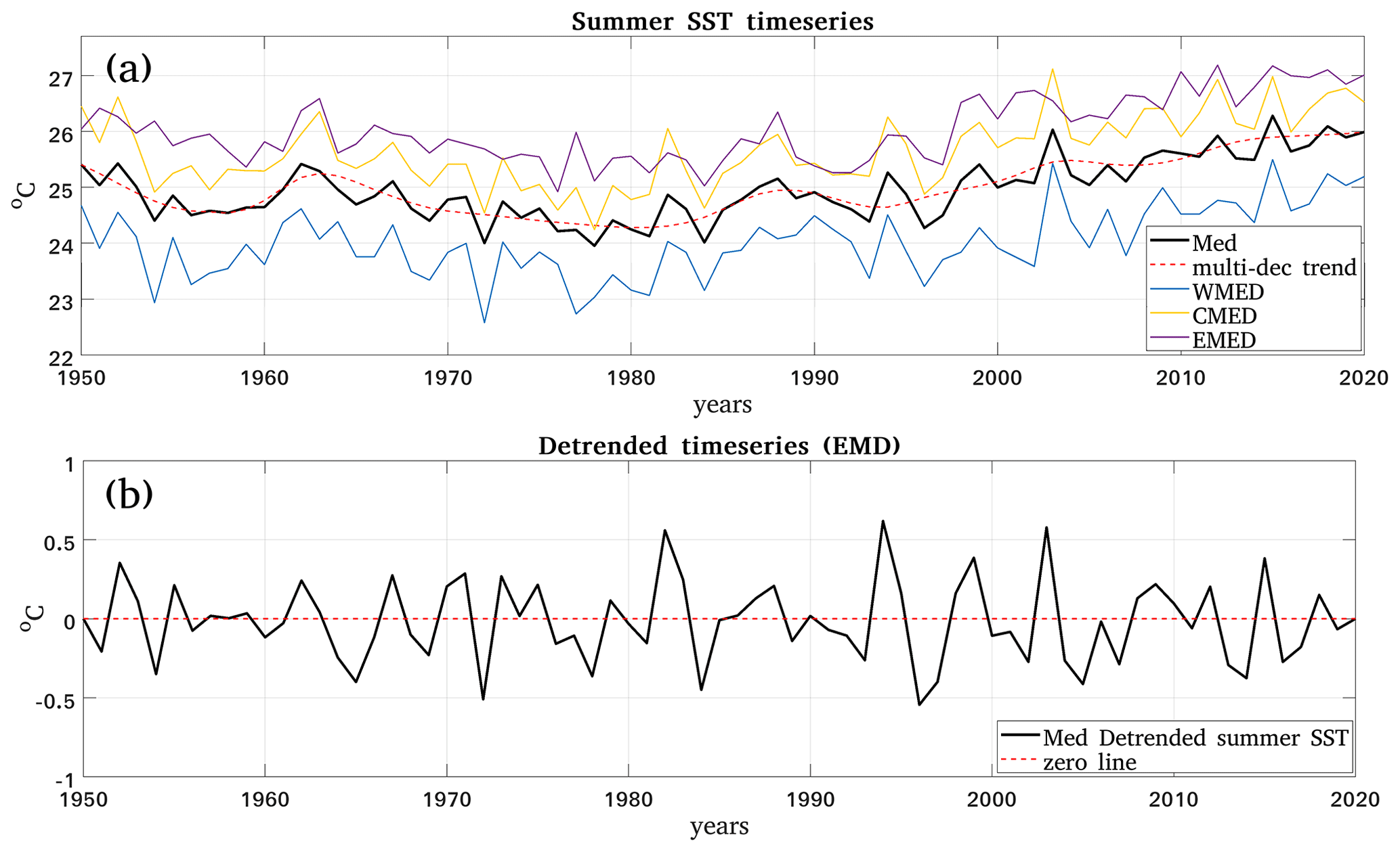
Figure 2 Example of applying the empirical mode decomposition (EMD) (Wu and Hu, 2006) to remove the multi-decadal trend from summer ERA5 SST data for the period 1950–2020: (a) domain-averaged mean summer SST values and multi-decadal trend (black line and dashed red line, respectively). Mean summer SST time series averaged for the western, central, and eastern sub-basins are also depicted in blue, yellow, and purple lines, respectively. The three considered sub-regions here are separated by the Strait of Sicily (forming a natural boundary itself) and a constant-longitude boundary at 22° E. (b) Detrended summer SST anomaly time series for the MS derived from subtracting the multi-decadal trend from the domain-averaged time series of (a).

Working with the detrended SST time series, the EMS identification becomes independent of the Mediterranean SST multi-decadal variability, including the warming trend observed over the recent decades (i.e. climate change signal). In this study, we use both the original and the detrended data to (i) gain insight into the actually warmest EMSs that the MS has experienced within 1950–2020 and (ii) understand the role of the subtracted signal, respectively. Differences are discussed throughout the Results section.

2.2.3 Marine heatwave identification

MHW detection was performed on the daily ERA5 SST dataset for the period 1950–2020, based on the MHW definition and detection methodology of Hobday et al. (2016) and using the MATLAB toolbox provided by Zhao and Marin (2019). The reference period used to create the daily climatology is 1983–2012. The choice of the climatological period follows the general recommendation of a minimum of 30-year period for the computation of the climatology and thresholds for MHW detection (Hobday et al., 2016). Sensitivity tests using different climatology periods show some differences in the resulting MHW properties (not shown). However, the MHW analysis in this study aims to investigate potential changes in main MHW characteristics during extreme seasons, rather than provide a thorough discussion of MHW properties in the MS. Therefore, such discrepancies resulting from different climatological periods are not considered significant in the scope of the present study. In addition, the availability of satellite SST data during the selected climatological period allowed for detecting MHWs using this dataset as well. This task was performed to examine whether the reanalysis dataset can produce similar results with the observations for the recent decades. MHW detection results based on reanalysis (ERA5) and observational (CMEMS) SST for the common period were found to be very similar (not shown). For consistency reasons, the same climatological period (1983–2012) was used when applying the same methodology for detecting MHWs based on the detrended SST data.

To focus on summer MHWs, we isolated events with their onset and end day falling within the JAS summer period and then computed their mean summer properties (intensity, duration, frequency). The fixed temporal length of a season inevitably leads either to the underestimation or overestimation of the number of MHWs, depending on whether events begin and end entirely within the season. We chose to include only events fully within the season to inter-compare MHW properties between extreme and non-extreme summers over the 71-year period. Both approaches (including fully within-season MHWs or considering partly within-season MHWs) have been tested and results do not significantly alter our conclusion on whether and where enhanced MHW conditions are found during EMSs (not shown). In addition to the intensity, duration, and frequency of summer MHWs, we also considered the number of MHW days falling within JAS periods, being free of the aforementioned limitation.

Means of MHW properties are produced by averaging over all summer events within the 71 summers of the study period. In turn, the EMS anomalies of the examined MHW properties are computed by subtracting the climatological (summer) mean from the mean over the four EMSs, at each location. Averages over the 71 summers and over the 4 EMSs represent the mean seasonal conditions of (i) all summer MHWs within the study period and (ii) the MHWs occurring within EMSs, respectively, both not expected to be indicative of the most extreme MHW conditions. MHWs may promote the formation of an EMS either by being more frequent, of greater duration, or of greater intensity than usual, thus, contributing in different ways with positive SST anomalies to the seasonal SST being the focus of this study.

2.2.4 Air–sea heat fluxes in extreme marine summers

This section presents the methodology we followed to study the role of air–sea heat fluxes as potential EMS drivers. Heat exchange at the air–sea interface may be quantified through the net surface heat budget equation, as follows:

$$\begin{array}{}\text{(8)}& Q_{\mathrm{net}}=\mathrm{LH}+\mathrm{SH}+{\mathrm{SWR}}_{\mathrm{net}}+{\mathrm{LWR}}_{\mathrm{net}},\end{array}$$

where Q_net is the net surface heat flux, and LH, SH, SWR_net, and LWR_net are the latent heat flux, sensible heat flux, and the net short-wave and long-wave radiation, respectively.

To investigate the role of surface heat fluxes during EMSs, we first compute, for each grid point, the mean EMS anomaly of Q_net and its components with respect to climatology. This is done by subtracting the mean summer value of the examined variable over the 71-year study period from its mean value over the four locally detected EMSs. Notably, a summer Q_net anomaly value represents the cumulative effect of surface fluxes on the sea surface within a summer season (i.e. a heat surplus or deficit during that summer relative to climatology). Specifically, sequential warming and cooling effects of Q_net on the sea surface are expected to occur during a season and, in turn, be enhanced or counterbalanced by atmospheric and/or oceanic processes. Therefore, a positive (negative) seasonal Q_net anomaly of an EMS does not necessarily reflect a driving (opposing) role of Q_net in forming this EMS. To answer the question “what is the driving role of air–sea heat fluxes in the formation of EMSs?”, we need to focus on the role of Q_net in forming the SST anomalies that are responsible for making a summer extreme (on the basis of mean summer SST). On these grounds, in addition to examining seasonal heat flux anomalies, we propose a metric to quantify the contribution of Q_net during selected summer sub-periods. During the selected sub-periods, SST evolves towards greater SST anomalies, either through warming occurring at a greater rate than usual or through cooling occurring at a lower rate than usual. A more detailed description on the rationale and methodological steps for constructing the metric is included in Appendix A.

2.2.5 Extreme marine summer preconditioning

A warmer than usual upper-ocean layer before the beginning of the summer season may favour the formation of an EMS. To explore the potential role of upper-ocean preconditioning in the development of an EMS, we examine the oceanic thermal conditions of the mixed layer prior to the JAS period. We choose June as the reference period to calculate the ocean heat content (OHC), considering it as indicative of the surface ocean “thermal state” before each summer. We compute the OHC of the mean mixed layer depth (MLD) for every June and the corresponding EMS anomalies. The EMS anomalies for OHC are computed at each grid point by subtracting the climatological OHC value for June, from the mean OHC value for June over the 4 EMS years (mean June before EMSs minus mean June of all years). OHC in this task is computed based on the following equation:

$$\begin{array}{}\text{(9)}& \mathrm{OHC}=\iiint \mathit{\rho }{C}_{p}T\mathrm{d}x\mathrm{d}y\mathrm{d}z,\end{array}$$

where ρ is the water density, C_p is the water heat capacity, and $T\left(x,y,z\right)$ is the 3D monthly mean (June) ocean temperature taken from the CMEMS Physics Reanalysis dataset. As the integration depth (MLD of each June) at each location varies interannually, vertical integration in Eq. (9) makes use of all T values that are available above the MLD of the specific location and month. To avoid inter-comparing OHC computed based on different integration depths (thus, different volumes of water) from summer to summer, we normalize the produced OHC values by dividing them with the mean MLD of the respective location and month. The produced anomalies are considered to be a (qualitative) preconditioning index for the EMS formation. Due to the temporal coverage of MLD data (1987–2019), MLD and OHC anomalies have been computed relative to mean values over this period, instead of the entire study period (1950–2020) used in the computation of anomalies for the rest of the examined variables in the paper. The impact of using a different reference period for these parameters has been examined and found to be negligible.

3 Results

3.1 Extreme marine summer substructures

The average rank day anomaly (RDA) of the four EMSs is computed for each grid point based on Eq. (2) and shown in Fig. 3a. The maximum EMS RDAs reach up to 2.5 °C in the western basin, within the Gulf of Lions and the Ligurian Sea and extending to the south, surrounding Sardinia. The Tyrrhenian and the central Adriatic seas follow with maximum anomalies reaching up to 1.8 °C. In the rest of the basin, RDAs are of the order of less than 1.4 °C, with its minimum values found in the southernmost areas of the Ionian Sea.

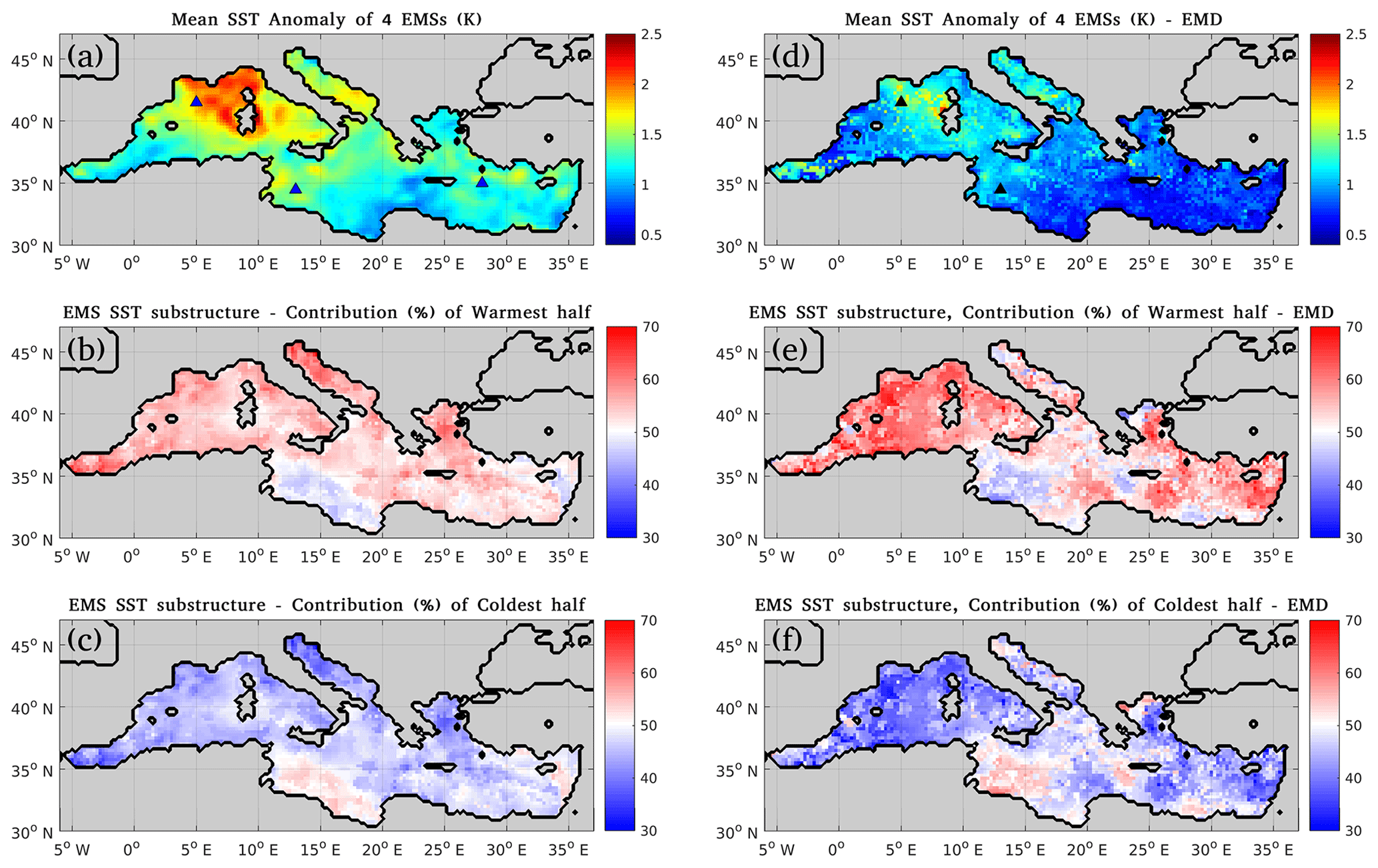
Figure 3 (a, b, c) Panel (a) shows mean extreme marine summer (EMS) rank day anomaly (RDA) field based on ERA5 SST 1950–2020, (b) percentage of contribution to the EMS RDA of the warmest half of the EMS RDA distribution, and (c) percentage of contribution to the EMS RDA of the coldest half of the EMS RDA distribution. (d, e, f) Same as (a), (b), and (c) but using the detrended dataset. Blue triangles represent the locations of the selected grid points discussed in this section.

To gain insight into the SST substructures over the basin, Fig. 3b and c show the fractional contributions of the warmest and the coldest half of the RDA distribution to the mean EMS RDA, based on Eqs. (3)–(4). The warmest half contributes the most in the greatest part of basin. This suggests that EMSs are primarily formed due to the warmer summer days being warmer than normal in most MS areas. The maximum contribution from the warmest part reaches up to 70 % (North Adriatic, Alboran Sea). On the other hand, the coldest half contributes the most, with an order of 55 %, only within an area of the southern–central basin, close to the African coasts (Fig. 3b, c). These results distinguish the EMSs in this area being primarily formed due to the colder days being warmer than normal (further discussed in Sect. 3.3).

When the multi-decadal trend is removed, smaller SST anomalies in EMSs are found in the entire MS, compared to the original dataset (Fig. 3a, d). The original and detrended RDA fields differ by approximately 0.5 °C. This difference is expected, as the detrended dataset is free of the warming trend in the MS. The spatial distribution of the RDAs and the corresponding fractional contributions of the coldest or warmest parts of the SST distribution are similar to the ones obtained when using the original dataset (left vs. right column in Fig. 3). Despite the difference in the RDA magnitude, both fields in Fig. 3a and d depict a west–east RDA gradient with the largest RDA values in the western Mediterranean Sea. In both fields, RDA peaks are found in the Gulf of Lions and the Ligurian Sea, followed by the Adriatic Sea. Similarly, the contributions of the coldest and warmest part to the EMS RDA present very small differences (Fig. 3b, c compared to Fig. 3e, f).

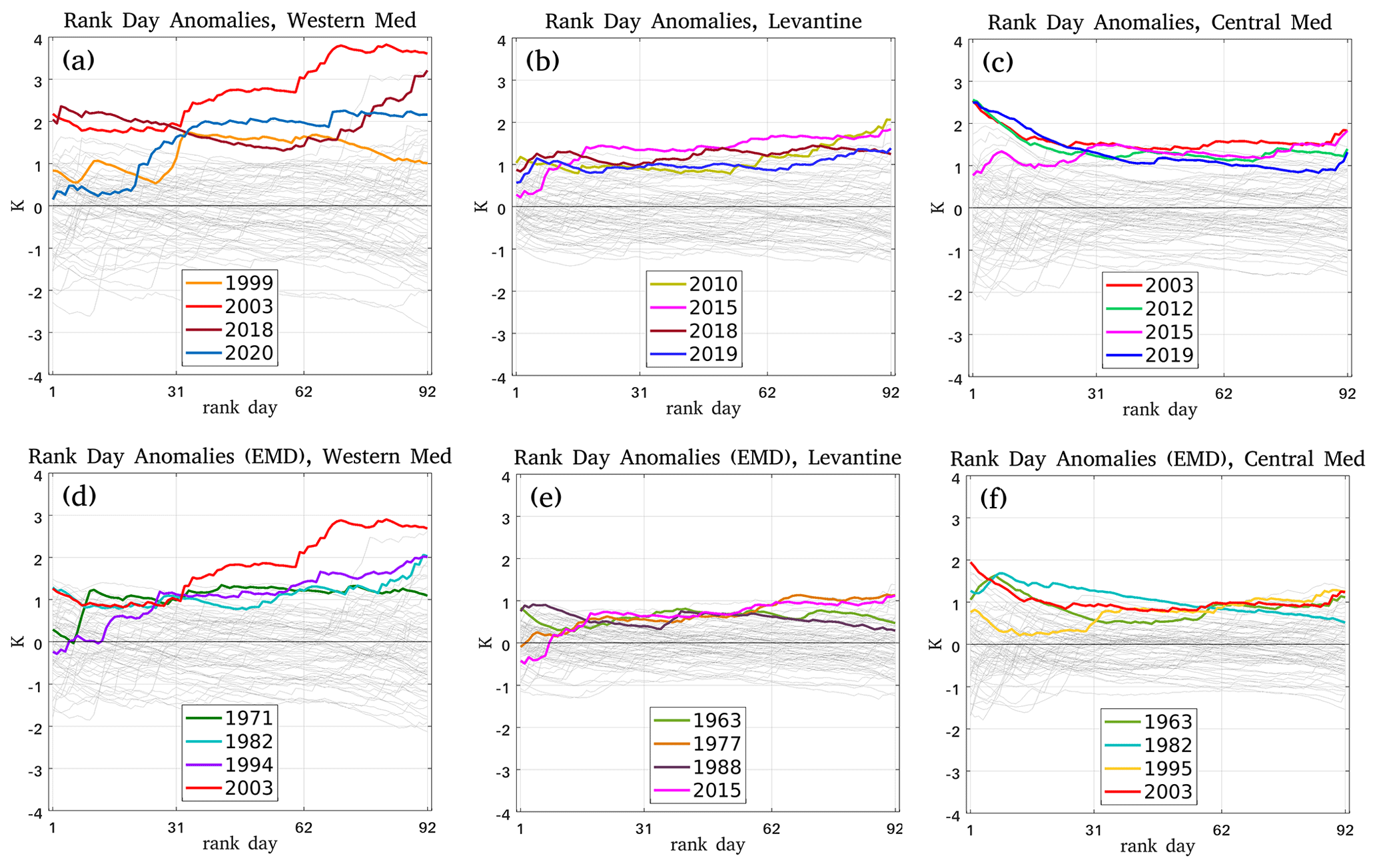
Figure 4 SST substructures of EMSs identified within 1950–2020 at three example locations: (a, d) southern of the Gulf of Lions (41.5° N–5° E), (b, e) in the central Levantine Sea (35° N–28° E), and (c, f) eastern of the Gulf of Gabes (34.5° N–13° E) using the original (top row) and the detrended (bottom row) summer SST dataset. Coloured lines stand for EMSs, grey lines for non-EMSs. Horizontal axis shows the 92 rank days of the JAS summer season (there is no temporal order).

To gain insights into the SST substructures of different EMSs, in Fig. 4 we provide examples of different patterns for three grid points of the domain (locations marked on maps of Fig. 3). In particular, Fig. 4a shows the SST substructures for a grid point located in the Gulf of Lions (41.5° N–5° E). Mean EMS RDA at this location reaches up to 1.86 °C. The EMS 2003 stands out with the larger mean RDA among all EMSs. At the same location, the summer of 2020 presents a similar SST substructure but with anomaly values of smaller amplitude. The EMSs 1999 and 2018 present a varying contribution to the mean RDA from the different parts of the SST distribution at this location. Regardless of the variability of the SST substructures among the four EMSs, the largest contribution to the mean EMS RDA at this location comes from the warmest part of the SST distribution (higher half of rank days), as it explains 59 % of the mean EMS RDA.

Same as the location in the western basin, the grid point in the central Levantine (35° N–28° E) presents higher RDAs in the warmest rank days (Fig. 4b). However, RDAs for all EMSs at this location present a similar distribution. The mean EMS RDA here is of 1.18 °C and results from a slightly higher contribution from the warmest than from the coldest rank days, as the former explain 57 % of the EMS RDA. The 4 EMS years here fall into a more recent period of our climatology compared to the ones identified in the other example locations. This is due to the non-uniform warming trend in the MS. In particular, the eastern part of the basin (EMED) presents larger positive SST trends (Shaltout and Omstedt, 2014; Pastor et al., 2020; Pisano et al., 2020). Consequently, when using the original (non-detrended) dataset we expect the EMSs in the EMED to fall in more recent years compared to the EMSs identified in the western part of the basin (WMED).

Figure 4c presents the EMS SST substructures at a grid point located north of the Tunisia coasts (34.5° N–13° E). In contrast to the other two example locations, the largest contribution to the mean EMS RDA here (1.4 °C) comes from the coolest days of these summers being anomalously warm, as they explain 54 % of the mean EMS RDA (Fig. 4b). This pattern is observed in three (out of the four) EMSs, while the EMS 2015 presents an almost uniform positive SST shift during the season. The year 2003 stands out again with the largest mean RDA, with its maximum value occurring in the lowest rank of this summer (2.6 °C).

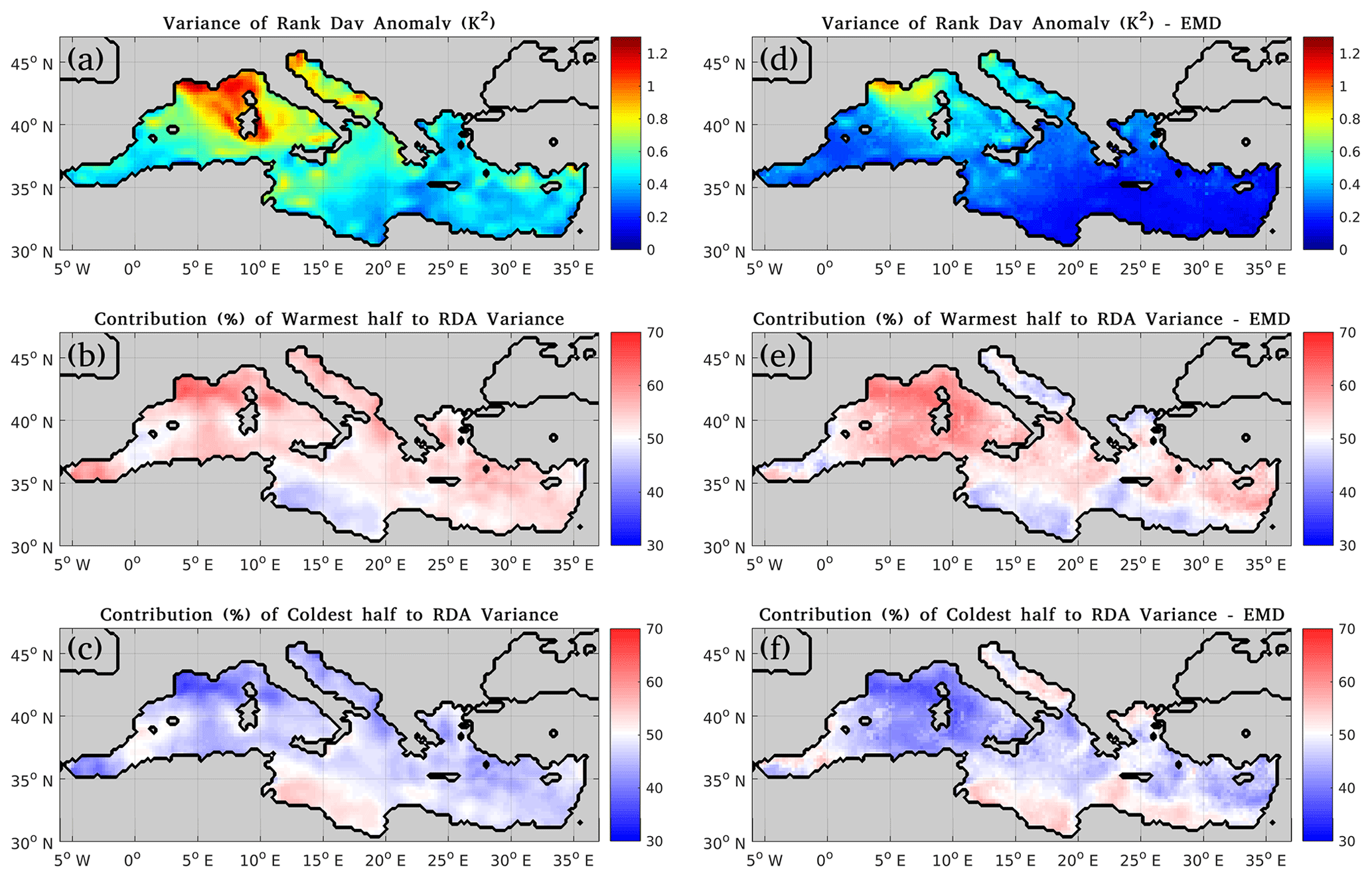
Figure 5 (a, b, c) Panel (a) shows variance of RDA based on all summers within 1950–2020, (b) percentage of contribution to the RDA variance of the warmest half of all summer rank days within 1950–2020, and (c) percentage of contribution to the RDA variance of the coldest half of all summer rank days within 1950–2020. (d, e, f) Same as (a), (b), and (c) but using the detrended dataset.

To examine the role of the local rank day SST variability in forming the observed EMS substructures, we first compute the variance of the RDA of all summer seasons within the study period based on the Eq. (5) (Fig. 5a). The spatial distribution of the variance of RDA is remarkably similar to the mean EMS RDA field in Fig. 3a. In particular, large seasonal SST anomalies are found, as generally expected, in locations of large rank day SST variability. Results come in agreement with Shaltout and Omstedt (2014) that examined the SST variability in the basin showing that the maximum and minimum seasonal stability are found close to the southern Levantine sub-basin and the Gulf of Lions, respectively.

This RDA spatial pattern (west–east gradient) is also present in the RDA variance field of the detrended dataset (Fig. 5a vs. Fig. 5d). This suggests that a similar rank day variability pattern in the two datasets modulates the seasonal SST anomalies observed in EMSs. Additionally, the contribution fields from the two parts of the RDA distribution of all summer seasons to the RDA variance present only slight differences in certain areas compared to the original dataset (Fig. 5b, c vs. Fig. 5e, f). In particular, in the detrended dataset, locations where the coldest rank days contribute to the RDA variability more than 50 % are not restricted in the southern–central area north of the African coasts as in the original dataset. It is also the central Adriatic, part of the southern Levantine, and the North Aegean seas that exhibit a slightly enhanced contribution of the cool summer days to the RDA variability (Fig. 5e, f).

We then calculate the fractional contribution of the coldest and the warmest half of the ranked summer days to the RDA variance computed for all 71 summers, based on the Eqs. (6)–(7) (Fig. 5b, c). The contribution of the warmest (coldest) half of all daily summer SST values to the RDA variance is very similar to the contribution of the warmest (coldest) half of the EMS RDAs to the total EMS RDA (Fig. 5b, c vs. Fig. 3b, c). In other words, the locations where the warmest (coldest) part of the rank day distribution has higher spread experience EMSs primarily due to the contribution of the warmest (coldest) part of the rank day distribution of EMSs.

This may be observed in more detail in the example cases presented in Fig. 4a–c, considering also the grey lines that correspond to the rest of the years (non-EMS years). At the location at 41.5° N–5° E (Fig. 4a), the warmest part of the RDA distribution, which contributes the most to the EMS RDA, also contributes the most (60 %) to the seasonal variance of RDAs (0.85 °C²). In other words, this is the part presenting the largest RDA spread in the rest of the years as well (Fig. 4a). Similarly, at the location at 35° N–28° E, the highest rank days which contribute the most to the mean EMS RDA are also the most varying from summer to summer within the study period, explaining 56 % of the seasonal variance (0.43 °C²) (Fig. 4b). In contrast, at the location 34.5° N–13° E, the coldest half of summer rank days, which contributes the most to the mean EMS RDA, exhibits greater RDA variability over the 71 summers, accounting for 55 % of the seasonal variance (0.56 °C²) (Fig. 4c). In all cases, the part of the RDA distribution that contributes the most to the EMS RDA is the one presenting the largest spread climatologically.

It is noteworthy that the observed common spatial pattern of SST substructures in the original and the detrended dataset (Fig. 3a–c vs. Fig. 3d–f) results from different combinations of EMSs. To better illustrate this, the SST substructures in the three example cases discussed above are very similar for the original and the detrended dataset, despite the actual EMSs being warmer than the ones identified using the detrended dataset (Fig. 4a–c vs. Fig. 4d–f, respectively). Three out of the four identified EMS years in all example locations differ between the original and the detrended dataset. Despite this, at each location, the part of the SST distribution contributing the most to the RDA is the same in the two datasets, and it is the most variable climatologically.

In addition, SST substructures in EMSs seem to be independent of the selected study period. Sensitivity tests performed for different sub-periods show a consistent statistical behaviour (similar spatial distribution of EMS substructures) of the detrended SST dataset compared to the original one (not shown).

This analysis suggests that EMSs are formed based on a “background” SST substructure field, largely depending on the climatological ranked daily SST variability in the MS. On top of this field, the multi-decadal signal adds extra warming in the basin, resulting in warmer EMSs.

3.2 The role of marine heatwaves in extreme marine summers

Following the SST substructures of EMSs presented in the previous section, this section further informs on EMS characteristics by investigating MHWs during EMSs. We first present basic MHW properties during summers in the MS, as obtained from the reference SST dataset for the period 1950–2020 (Sect. 3.2.1). Then, we examine the relative role of MHWs in EMSs by means of changes in MHW properties during EMSs with respect to mean summer MHW conditions (Sect. 3.2.2).

3.2.1 Detection of summer marine heatwaves in ERA5

Summer MHWs are more intense in the northern parts of each Mediterranean sub-basin (Fig. 6a). Mean summer MHW intensity (mean SST anomaly during a MHW with respect to local climatology) reaches its maximum values (approximately 2.6 °C) in the north-western part of the basin. The Adriatic Sea displays the second highest MHW intensity (approximately 2 °C). Values of about 1.5–2 °C mostly appear within the latitudinal zone between 35 and 42° N in the Tyrrhenian, the Ionian, and the Aegean seas. The lowest mean intensity appears off the African coasts, extending from 15° E eastwards. Striking similarities between the MHW mean intensity (Fig. 6a) and the SST RDA variance field (Fig. 5a) reflect the expected dependency of warm extremes on the local SST variability. This is observed particularly in the north-western regions, indicating that the more variable the daily SST values over the studied summers are, the more intense both EMSs (as shown in Sect. 3.1.2) and MHW events are.

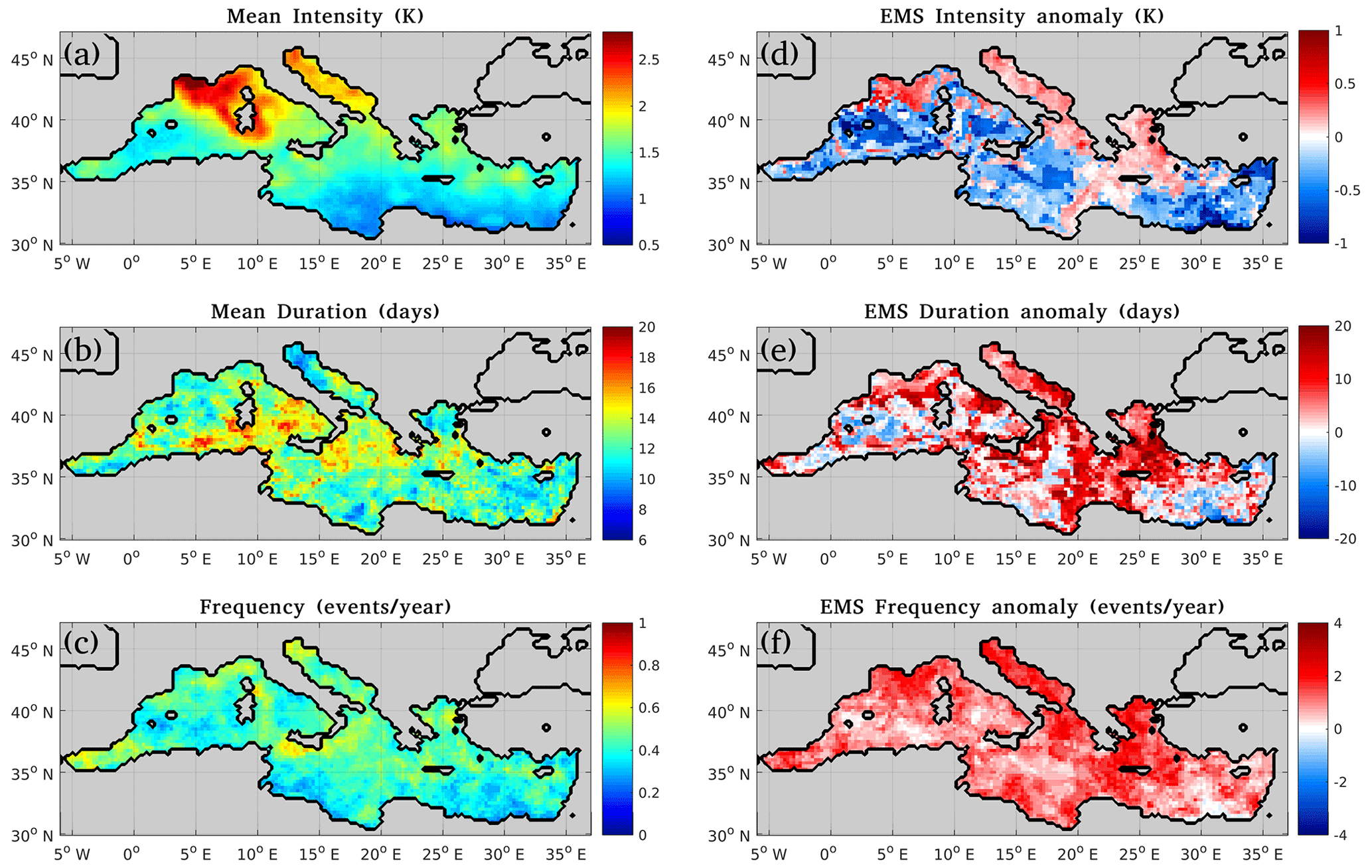
Figure 6 Summer marine heatwave (MHW) properties in the Mediterranean Sea in the period 1950–2020 and their anomalies in extreme marine summers (EMSs). (a, b, c) Mean intensity (a), mean duration (b), and mean frequency of occurrence (c). (d, e, f) EMS anomalies of mean intensity (d), mean duration (e), and mean frequency of occurrence (f) with respect to the mean summer values displayed in (a), (b), and (c).

Average MHW duration in the largest part of the basin ranges between 10 and 15 d (Fig. 6b). Longer-lasting events (up to 20 d) are found in discrete spots in the Tyrrhenian, the Ionian, and to a lesser extent in the southern Aegean Sea. It is noteworthy that areas such as the Gulf of Lions, the Adriatic, and the North Aegean Sea, where MHW intensity is high, tend to present shorter mean duration values, varying between 8–12 d. Concerning summer MHW frequency, in most areas a MHW occurs approximately every two summers (Fig. 6b), while the rest of the basin experiences MHWs slightly more or less frequently (every 1–3 years).

Our results on MHW analysis are in agreement with prior studies. Indeed, Darmaraki et al. (2019a) showed that mean MHW intensity computed from observations and model data for the period 1982–2017 present the same spatial distribution in the basin, highlighting the northern regions of each sub-basin and particularly the north-western MS as the areas of the highest MHW intensity. The significantly smaller mean intensity values in the entire basin in Darmaraki et al. (2019a) result mainly from their definition for MHW intensity as the mean SST anomaly over the event duration with respect to the selected temperature threshold, instead of the local climatology used in this study following Hobday et al. (2016).

MHW analyses based on satellite SST observations by Ibrahim et al. (2021) and Juza et al. (2022) for the period 1982–2020 as well as Dayan et al. (2023) for the period 1987–2019 are also consistent with the current findings for summer MHWs, despite their shorter reference periods and the season-independent analysis. However, all aforementioned studies report larger MHW durations in the south-eastern MS compared to our results. This difference is mostly related to our choice to focus on summer MHWs that begin and decay within the JAS summer period. Taking into account all events throughout the year, similar MHW duration values with these studies are reproduced (not shown).

3.2.2 Marine heatwave properties during extreme marine summers

To understand the role of MHWs in EMSs, this section presents the EMS anomalies of MHW properties with respect to their mean summer values. MHW conditions in EMSs present positive intensity anomalies mostly in the northern parts of each sub-basin, where the mean MHW intensity is generally larger (Fig. 6a vs. Fig. 6d). MHW intensity anomaly values in EMSs in the north-western Mediterranean, the Adriatic, the Aegean, and (part of) the Ionian seas reach up to 0.5 °C. Surprisingly, in the rest of the basin, MHWs occurring within EMSs exhibit lower intensity relative to the mean summer conditions (negative anomalies in Fig. 6d). In the same areas though, the MHW frequency (number of events per summer) is greater within EMSs than usual (Fig. 6e). It should also be noted here that MHWs do not occur during every summer of the study period, but they occur at every single grid point during EMSs; hence there are no spatial gaps in the anomaly maps of Fig. 6d–f.

MHWs within EMSs appear longer lasting in most MS regions and occur more frequently across the entire MS (Fig. 6e and f, respectively). The greatest duration anomalies exceed 15 d and are mostly located in the Aegean, the Ionian, and the Adriatic seas and to a lesser extent in specific spots in the western Mediterranean Sea. Few small areas in the western basin and the south-eastern Levantine Sea present slightly smaller mean event duration in EMSs (Fig. 6e). The frequency anomalies are positive almost in the entire basin, with most areas experiencing at least one additional event per summer during EMSs, compared to mean summer MHW conditions (i.e. compared to the normally expected number of events per summer) (Fig. 6f). The largest frequency anomalies appear in the Aegean (approximately three extra events per summer during EMSs), followed by the Adriatic and the north-western MS.

The relative contribution of MHWs during EMSs with respect to mean summer MHW conditions can also be expressed in terms of MHW days, through the percentage of MHW summer days occurring within EMSs. Results show that at least 25 % of the MHW days detected within the 71 studied summers occur within the 4 EMSs at each location (Fig. B2a). This percentage varies from 25 % to 55 % across the basin, with the central and eastern basin presenting the greatest values. This analysis suggests a more pronounced role of MHWs during EMSs in these areas, this time by means of temporal coverage of MHW conditions.

To understand how the revealed SST substructures of EMSs (Sect. 3.1) are related to MHW occurrences, we also attribute MHWs to different parts of the RDA distribution. Figure B2b shows the percentage of MHW days falling within the warmest part of the RDA distribution during EMSs (the corresponding percentage for the coldest part is simply the remaining percentage). This figure reveals that the majority of MHW days during EMSs take place within the warmest half of the RDA distribution in the entire basin. Particularly in northern regions (north-western MS, Adriatic and Aegean seas), very large percentages (locally exceeding 95 %) of MHW days fall within the warmest part of the RDA distribution, while high percentages are also encountered in the Alboran and the Ionian Sea to the southwest of Crete. The lowest values, of about 50 %, are observed in certain spots in the eastern Levantine Sea, showing that MHW days during EMSs tend to be uniformly distributed over the warmest and the coldest part of the SST distribution at these locations.

Furthermore, the northern sub-regions and south-eastern Ionian Sea where the vast majority of MHW days in EMSs occur within the warmest part of the summer are also the areas presenting the higher EMS anomalies for all MHW properties (Fig. 6d–e vs. Fig. B2b). This suggests that the more intense, more frequent, and longer-lasting events observed during EMSs in these areas occur mainly within the warmest part of the SST distribution. Even in the south–central basin where the lower rank days (i.e. colder days) contribute the most to the observed EMS RDA (Fig. 3c), nearly 70 % of MHW days fall within the higher rank days of EMSs (Fig. B2b). In other words, although the warmer than usual cool summer days are the most responsible for the elevated mean summer SST in that region, MHW conditions there occur mainly during the warmest EMS days.

When the multi-decadal signal is removed, MHWs are basin-wide slightly less intense, while the intensity spatial distribution is remarkably similar between the original and the detrended dataset (not shown). This reflects the positive contribution of the multi-decadal signal to the observed sea surface warming, this time specifically via the SST anomalies caused by MHWs. During EMSs, the main difference in MHW properties between the two datasets is that the northernmost MS regions in the detrended dataset do not stand out in the EMSs as in the original one. In particular, when long-term trends are removed, it is the Aegean, the Tyrrhenian, and certain areas in the Ionian Sea that exhibit increased MHW properties during EMSs compared to climatology (not shown).

3.3 Investigation of potential extreme marine summer drivers

This section focuses on the role of air–sea heat exchanges during EMSs while it also discusses other physical mechanisms related to the EMS formation. Its content is structured as follows: we first present and discuss the seasonal anomalies of Q_net and its components for EMSs, relative to their mean summer value over 1950–2020 (Sect. 3.3.1). This task is complemented by examining wind and MLD in EMSs, as well as the preconditioning factor introduced in Methods. Next, we investigate the role of the multi-decadal variability in our findings for surface heat fluxes during EMSs (Sect. 3.3.2). In the subsequent section, we explore the meaning of using mean EMS values in this analysis, considering that differences are expected among the four EMSs detected at each location (Sect. 3.3.3). We then quantify the driving role of air–sea heat fluxes in the formation of EMSs. To achieve this, we use the proposed metric described in Methods and Appendix A, to compute the contribution of Q_net to the SST changes that are responsible for making a summer extreme (Sect. 3.3.4). Finally, we provide an illustrative example on quantifying the role of Q_net during a specific EMS based on this metric (Sect. 3.3.5).

3.3.1 Air–sea heat flux anomalies in extreme marine summers

Q_net anomalies in EMSs display a non-uniform distribution over the basin (Fig. 7a). Interestingly, positive anomaly values (i.e. heat gain or reduced loss from the sea surface) appear only in certain areas, most of which are in the northern flanks of the Mediterranean basin. The eastern Aegean, a part of the central Levantine, the Adriatic Sea, and the western part of the Gulf of Lions present greater positive anomalies reaching up to 15 W m⁻². Consistent with this finding, these are the areas presenting a significant negative correlation between SST and the net heat loss from the sea surface, as shown by Shaltout and Omstedt (2014) for the period 1982–2012. Moreover, positive Q_net anomalies appear mainly in areas where enhanced MHW conditions in EMSs were detected (northern Mediterranean regions and particularly the Aegean and the Adriatic seas; Fig. 7a vs. Fig. 6d–f). This similarity is at least partly attributable to the widely explored driving role of air–sea heat fluxes in the formation of MHWs (e.g. Holbrook et al., 2020; Sen Gupta et al., 2020; Schlegel et al., 2021; Vogt et al., 2022) and is further analysed in Sect. 3.3.4.

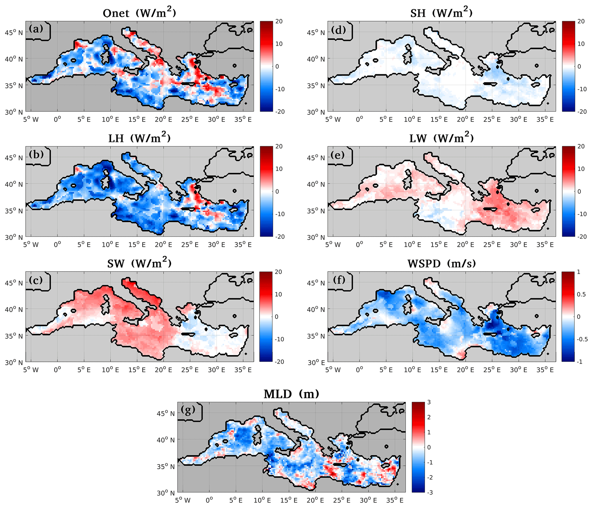
Figure 7 Extreme marine summer (EMS) anomalies of (a) Q_net, (b) latent heat flux, (c) net short-wave radiation, (d) sensible heat flux, (e) net long-wave radiation, (f) wind speed at 10 m, and (g) ocean mixed layer depth (MLD); EMS anomalies are computed with respect to their mean summer state based on 1950–2020 for all parameters except for MLD where the 1987–2019 baseline period was used. Downwards fluxes have been considered positive, so positive heat flux EMS anomaly values correspond to either heat gain or reduced loss from the sea surface.

The way each of the four Q_net components contributes to the net heat balance in EMSs is highly variable throughout the basin (Fig. 7b–e). However, we observe a dominant role of LH flux, as in most of the basin it accounts for more than 80 % of the Q_net anomalies. The Adriatic, parts of the Ionian Sea, and some extra sites are exceptions on this pattern. We also distinct two primary mechanisms leading to positive Q_net anomalies: the reduced LH loss and the increased net SWR. The former is mostly met in the Aegean and Levantine seas and in the western part of the Gulf of Lions (Fig. 7a, b) and the latter in the Adriatic Sea (Fig. 7a, c). In the following, we discuss how the different Q_net components, wind and MLD, behave during EMSs in the aforementioned areas.

The positive Q_net anomalies observed in the eastern Aegean and in the central Levantine seas are mainly formed by reduced LH losses, as the positive LH flux anomalies explain more than 70 % of the Q_net anomalies in the area (Fig. 7a, b). Although wind in EMSs appears reduced almost in the entire basin, it is in the EMED and particularly in the Aegean Sea where the largest negative anomalies appear (Fig. 7f). In fact, positive LH flux anomalies appear in the EMED where the northerly etesian winds persistently blow during the summer period (from the north-east (north-west) in the northern (southern) Aegean with maximum values in the central Aegean; Nittis et al., 2002). This suggests that the reduced strength (or eventual ceasing) of the etesian winds plays a crucial role in the EMS formation in the area through the suppression of LH loss from the sea surface and the consequent rise in SST. SH flux (Fig. 7d) and net SWR anomalies (Fig. 7c) in the eastern Aegean and the central Levantine seas are negative and correspond to −20 % and −10 % of the positive Q_net anomalies in the area, respectively. Finally, the EMED and particularly the Aegean Sea present the highest positive LWR anomalies (Fig. 7e) in the basin. LWR anomalies in the Aegean Sea correspond to nearly 60 % of the Q_net anomalies in the area. The net SWR deficit in the same area suggests that increased cloudiness over the Aegean and the Levantine seas in EMSs has probably formed the observed net LWR surplus (further discussed below).

In the western part of the Gulf of Lions, the positive Q_net anomalies are determined by reduced LH losses as well as increased SWR (Fig. 7a, b, c). The contributions from the positive LH and SWR anomalies to the overall heat gain are approximately equal (50 %) in this area. Here, winds during EMSs (north-westerly mistral and tramontane) present negative anomalies (Fig. 7f) consistently with the observed suppression of LH fluxes. Negative MLD anomalies in the western part of the Gulf of Lions also imply wind-induced mixing reduction in the vertical (Fig. 7f, g). Notably, this area belongs to a much greater part of the MS that presents positive net SWR anomalies in EMSs and covers more than half of the basin, extending from the north-western to the central Mediterranean and the Adriatic Sea (Fig. 7c). The contribution of SH flux and net LWR in the overall heat gain detected in the area during EMSs appears non-significant (Fig. 7d, e).

In contrast to the two areas previously discussed, the positive Q_net anomalies appearing in the largest part of the Adriatic Sea are almost fully determined by the SWR anomalies (Fig. 7a, c). The LH flux here presents a negative contribution to the observed net heat gain (i.e. increased LH loss), apart from a small area close to the Strait of Otranto where positive LH anomalies contribute of about 20 % (Fig. 7a, b). The increase of LH loss during EMSs in the Adriatic Sea is smaller than the increase in net SWR in the area, which accounts for more than 100 % of the observed net heat gain. The positive anomalies of the net LWR and especially of the SH flux in the same area are of a much smaller magnitude compared to the other components, corresponding to a contribution of 30 % and 10 % to the Q_net anomaly, respectively (Fig. 7b–e).

Particularly during summers, winds blowing over the sea surface are expected to have a great impact on the MLD and SST evolution, as the upper ocean is highly stratified and thus more sensitive to atmospheric forcing variability (D'Ortenzio and Prieur, 2012). Indeed, wind during EMSs appears weakened in the largest part of the basin (Fig. 7f). It is found to exceed (marginally) the climatological mean value only in small areas in the northern parts of the Adriatic, east of Sicily, off the Libyan coast, and in the northern Aegean. In these areas, consistently with the enhanced wind speed, positive MLD anomalies imply stronger vertical mixing near the surface (Fig. 7g). MLD and wind speed anomalies tend to present the same sign, especially where large anomalies appear. For instance, west of Sardinia, off the eastern coasts of Tunisia, and in the Aegean Sea where large negative wind anomalies (i.e. reduced winds) are found, also MLD presents the largest negative anomalies (i.e. reduced MLD), though in more contained areas. Wind anomalies, being negative in most areas, display a less variable spatial distribution compared to the MLD anomalies (Fig. 7f, g). As thoroughly discussed in D'Ortenzio and Prieur (2012), wind affects the mixed layer of the MS at several spatio-temporal scales, thus making wind-driven processes hard to describe in a climatological context. Hence, we do not expect to reveal an indubitable cause–effect relation between wind and the mixed layer evolution by using mean seasonal wind speed and MLD anomalies. Despite these caveats, results show that wind and MLD anomalies tend to evolve consistently in most areas, suggesting that this approach is able to describe to a certain extent the wind effect in the stratification state at seasonal scale.

Understanding the role of net LWR anomalies in EMSs also bears some complexity. The skin SST-driven upwards LWR as part of the net LWR makes it difficult to reveal the responding/driving role of the net LWR component. To overcome this, we could separately examine the downwards LWR. However, this inevitably includes the downward radiation that specifically results from the lower atmosphere response to the sea surface warming (e.g. after a MHW occurrence) through increased humidity, as discussed in Vargas Zeppetello et al. (2019). This positive feedback mechanism renders the driving role of the downward long-wave component less clear. Nevertheless, important insight into the role of both LWR and SWR radiation fluxes components in EMSs can be obtained by examining Fig. 7c vs. Fig. 7e. These fields show that LWR and SWR anomalies (standing for net values from now on) in EMSs exhibit opposite sign in many areas across the basin.

The Aegean and part of the Levantine seas present negative SWR and positive LWR anomalies, suggesting increased cloudiness in these areas during EMSs. Indeed, positive EMS anomalies of total cloud cover derived from ERA5 are found in these areas (Fig. B5a) leading to increased downwards LWR and the observed reduced net LWR loss from the sea surface (Fig. 7e). In contrast, the largest part of the central and western basin presents positive SWR anomalies in EMSs. Particularly in parts of the Adriatic and the northern Ionian seas, the SWR surplus is responsible for the net heat gain observed in EMSs (Fig. 7a vs. Fig. 7b–e). Clear-sky conditions seem to favour EMSs in these areas, as implied by the reduced total cloud cover found in EMSs (Fig. B5a).

Results suggest that Q_net anomalies (either positive or negative) in EMSs are primarily formed by LH fluxes in most areas. The SWR is found to be the second most important Q_net component during EMSs, playing a crucial role in the western and central basin and particularly in the Adriatic Sea. Importantly, negative Q_net anomalies in EMSs are observed in a large part of the basin. In this regard, it should be noted that seasonal Q_net anomalies reflect the cumulative role of surface fluxes in EMSs, i.e. that the heat flux gained by the sea surface is smaller or larger than the upward heat flux during the season (relevant discussion in Methods, Sect. 2.2.4). Such information does not provide a safe conclusion on whether (and to what extent) Q_net drives EMSs. To fill this gap, in Sect. 3.3.4 we apply the proposed methodology (see Methods) for the quantification of the Q_net contribution in developing EMSs.

3.3.2 Air–sea heat fluxes using detrended data

To shed light on how the SST multi-decadal variability affects our findings for the role of surface heat fluxes during EMSs, we inter-compare the EMS Q_net anomalies derived from the original and from the detrended dataset. When the multi-decadal trend is removed, the EMS Q_net anomalies appear to be modulated by LH fluxes in the entire basin (Fig. B3). This constitutes the major difference compared to the original dataset where, in certain locations in the western and central basin, and particularly in the Adriatic Sea, clear sky conditions were found to play a major role during EMSs (Sect. 3.3.1).

In particular, positive SWR anomalies in EMSs in the western and central basin are much smaller in the detrended dataset and appear only in certain areas (Fig. B3). This is related to the positive trend of the summer net SWR since the mid-1970s being larger over the western and central basin (Fig. B4). As a consequence, SWR anomalies in these areas are larger in the original dataset where EMSs are identified mostly within the latest years. Results suggest that the key role of SWR in the EMSs actually experienced in western and central Mediterranean areas originates from the SWR long-term trend.

Wind speed EMS anomalies in the detrended dataset present the same sign and spatial distribution as in the original dataset (Fig. B3), further supporting the promoting role of low wind conditions for an EMS to occur, regardless of long-term variability. Nevertheless, wind during EMSs is less weakened in the detrended dataset. This magnitude difference is more pronounced over the Aegean and central Levantine seas, where also LH fluxes in EMSs are less suppressed in the detrended dataset (Fig. B3). The above is consistent with the documented weakening of the etesians (Tyrlis and Lelieveld, 2013; Poupkou et al., 2011; Dafka et al., 2018). In agreement with the literature, significant decreasing trend of wind speed in the EMED was also found based on the ERA5 JAS winds over the recent decades (not shown).

Summarizing, these findings suggest that in absence of multi-decadal variability, Q_net in EMSs is basin-wide dependent on the LH component. On top of this dependency, the actually observed Q_net during EMSs over the recent decades is further determined by the multi-decadal variability of (i) the SWR in the western and central basin and (ii) the wind-induced LH fluxes in the eastern basin.

3.3.3 Differences among extreme marine summers

Differences in the behaviour of surface heat fluxes are expected to exist among the four EMSs at a particular location and the mean EMS state presented in Sect. 3.3.1. To shed light on this, Fig. 8 illustrates how common a positive anomaly is for each of the examined heat flux components during EMSs. This is expressed as a fraction out of the four locally identified EMSs, ranging from 0 (no heat gain at all) up to $\mathrm{4}/\mathrm{4}$ (heat gain in all EMSs). The same approach is used to examine the occurrence frequency of weakened winds (Fig. 8b), reduced MLD (Fig. 8c), and preconditioning (Fig. 8d) in EMSs.

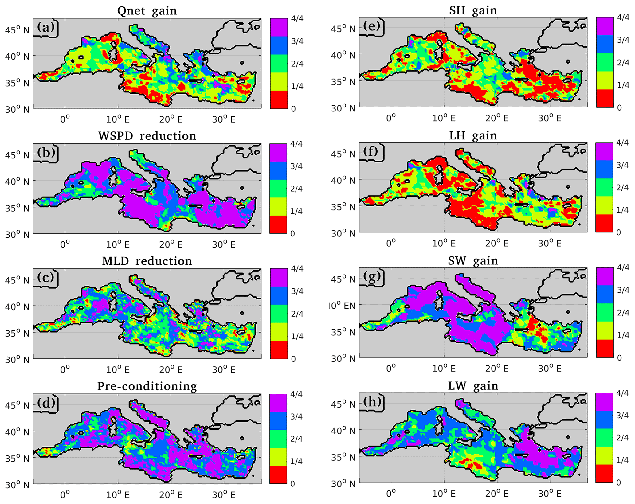
Figure 8 Percentage of the locally identified extreme marine summers (EMS) presenting (a) positive net heat flux anomalies, (b) reduced wind speed, (c) reduced mixed layer depth, (d) positive preconditioning index, (e) positive sensible heat flux anomalies, (f) positive latent heat flux anomalies, (g) positive net short-wave radiation anomalies, and (h) positive net long-wave radiation anomalies. Zero value (red) corresponds to a non-favouring role in any of the considered EMSs; $\mathrm{4}/\mathrm{4}$ (purple) corresponds to a favouring role in all EMSs.

The areas where positive Q_net anomalies in EMSs are more frequently met are the same as where the largest positive mean EMS Q_net anomalies were found (Fig. 7a vs. Fig. 8a). In particular, positive Q_net anomalies appear in at least three out of the four EMSs in the western part of the Gulf of Lions, the Adriatic Sea, and the Aegean Sea. Additionally, Q_net anomalies appear most commonly dependent on LH flux in parts of the Aegean and Levantine seas as well as in the western part of the Gulf of Lions, (Fig. 8a, f) and on SWR in the central and western basin (Fig. 8a, g), again consistent with the mean EMS anomaly fields.

Wind appears weaker in the majority of the EMSs ($\mathrm{3}/\mathrm{4}$ or $\mathrm{4}/\mathrm{4}$) with the exception of a few areas (Fig. 8b). In the Aegean Sea, low wind conditions contribute to surface warming through the suppression of both LH fluxes (Fig. 8f) and vertical mixing (Fig. 8c). The former mechanism is more common in the Aegean, in a few spots in the Levantine Sea, and in the western part of the Gulf of Lions than in any other location (Fig. 8f). In a large part of the central and western basin, LH fluxes rarely present positive anomalies, despite the reduced winds. In the same locations, SWR radiation appears increased in most EMSs, in line with the mean EMS findings.

Negative Q_net anomalies appear in every EMS in the Ligurian and the south–central as well as in a few specific spots in the western Mediterranean Sea, despite the systematically increased SWR. In these areas wind appears always reduced in EMSs (although not followed by decreased LH loss), while suppression of vertical mixing is observed only in half (or less) of the EMSs (Fig. 8c). On the other hand, the preconditioning index is found to play an important role in these areas, being positive in almost all EMSs (Fig. 8d).

Among the areas of negative Q_net anomalies, the south–central basin off the African coasts is where the coldest part of the SST distribution was found to contribute the most to the EMS SST anomalies (Fig. 3c). Relying on the increased mixed layer heat content before the beginning of almost every EMS in this area (Fig. 8d), we expect that the responsible cool summer days (being warmer than usual) are mostly the early-summer ones, rather than the late-summer ones. This is confirmed by looking into the area-averaged SST seasonal cycle (not shown). In all EMSs in this area, the early-summer (July) SST anomalies are the largest within the season. The increased mixed layer heat content in June is reflected in the positive SST anomalies of June while, also in May, SST in this area was found marginally larger than climatologically.

The temporal coverage of the modelled temperature and MLD inevitably limits the OHC calculation to only using the original dataset. This is because the EMSs identified based on the detrended SST time series often fall out of this temporal range, preventing their inclusion in the analysis. For this reason, a complementary task included the use of the detrended dataset only for locations that experience EMSs within 1982–2019, in order to examine whether the observed positive contribution of preconditioning results from the surface warming trend in the basin. In the region discussed above (south–central basin), increased upper-ocean heat content and spring SST values are observed before each EMS also in the detrended dataset, i.e. independently of the warming trend (not shown).

Upper-ocean heat accumulation is generally expected to precondition anomalously warm surface conditions (Marin et al., 2022). Indeed, in the greatest part of the basin, the preconditioning factor presents a positive contribution in more than half of the EMSs (Fig. 8d). Usefulness of this index is highlighted when examining single summers (as will be shown later in the exemplary case of EMS 2015). Even if it is positive in most cases, its contribution is often enhanced when and where there is no evident link between Q_net and the observed surface warming, thus revealing it constitutes an actually contributing EMS formation factor. Notably, occurrence frequency of preconditioning seems to differentiate in the Alboran Sea and the area surrounding the Strait of Sicily (Fig. 8d). Although horizontal advection is not investigated in this study, this finding potentially suggests that EMS preconditioning hardly takes place in areas of intensified circulation.

3.3.4 Quantifying the driving role of air–sea heat fluxes in the formation of extreme marine summers

In this section, we quantify the driving role of surface heat fluxes in the formation of EMSs. To this aim, we use the proposed metric (P_EMS) described in Sect. 2.2.4 and Appendix A. As explained therein, this metric quantifies the contribution of Q_net to the SST changes that are particularly responsible for making a summer extreme. During these EMS sub-periods, SST is kept above climatology via either (a) faster warming or (b) slower cooling compared to the corresponding climatological period. Positive (negative) P_EMS percentage values stand for a contributing (opposing) role of air–sea heat fluxes to the EMS formation.

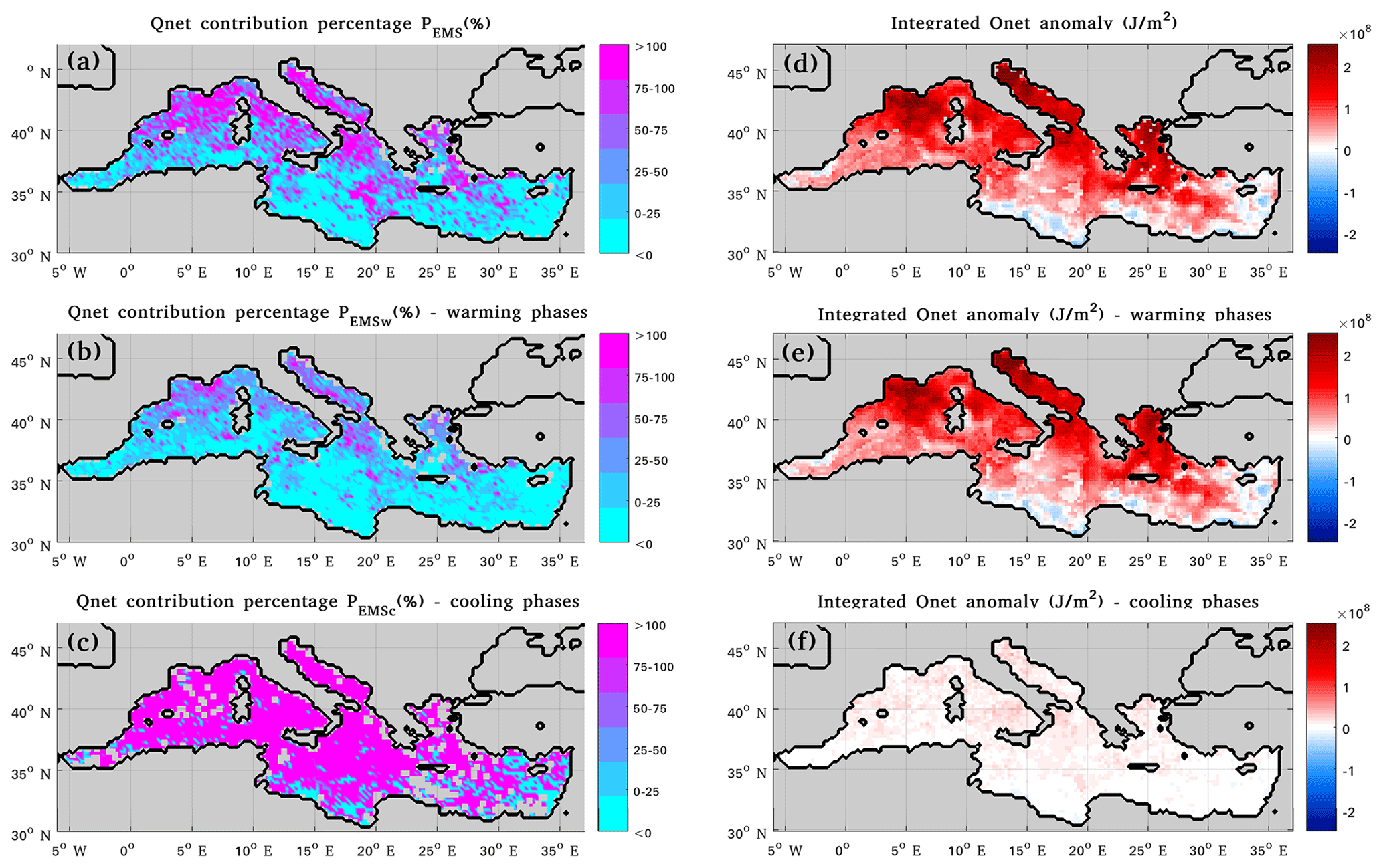
Figure 9 (a, b, c) Panel (a) shows P_EMS metric values (%) for the contribution of Q_net to the formation of EMSs (based on periods of positive cumulative SST anomalies and positive change in SST anomaly), (b) same as (a) but further focusing on warming phases ($P_{{\mathrm{EMS}}_{\mathrm{w}}}$), (c) same as (a) but further focusing on cooling phases ($P_{{\mathrm{EMS}}_{\mathrm{c}}}$). Note that positive (negative) values of metrics stand for a contributing (opposing) role of Q_net to the EMS formation. (d, e, f) Panel (d) shows integrated Q_net anomalies during the periods selected for the P_EMS computation; (e) same as (d) but further focusing on warming phases, and (f) same as (d) but further focusing cooling phases. Note that $P_{{\mathrm{EMS}}_{\mathrm{w}}}$ and $P_{{\mathrm{EMS}}_{\mathrm{c}}}$ percentages in (b) and (c) are relative to different reference periods (the selected warming and cooling phases, respectively; thus, their sum is, by construction, not expected to be equal to P_EMS in (a). Downwards fluxes have been considered positive, so positive anomaly values in (d)–(f) correspond to either heat gain or reduced loss from the sea surface during the selected phases. Sum of (e) and (f) equals the sum of Q_net anomalies in all selected phases (d).

P_EMS metric values in the MS are presented in Fig. 9a. Results reveal a crucial role of Q_net in driving EMSs in the northern half of the basin where the highest contribution percentages are encountered. A latitudinal gradient of P_EMS is generally observed in the basin: negative contribution percentages are found along the African coasts, while positive percentages of increasing value are found while moving towards northern MS areas. In positive P_EMS areas where air–sea heat fluxes do not entirely explain the observed change in SST anomalies (i.e. 0<P_EMS < 100 %), other mechanisms are expected to work complementarily (i.e. towards greater SST anomalies). Wind-induced mixed layer shoaling likely contributes in such cases, as suggested by negative wind speed and MLD anomalies (e.g. in Balearic and Aegean seas; Fig. 7f, g). P_EMS commonly exceeds 100 % mainly in northern Mediterranean regions (e.g. in Ligurian, Adriatic, North Aegean seas), meaning that additional processes (e.g. currents, vertical mixing) are expected to counteract the extra heating caused by surface fluxes in these cases. Negative P_EMS values in the southern regions reveal that air–sea heat exchanges work against the SST anomalies that are mostly responsible for the EMS formation; hence oceanic processes are expected to drive EMSs in these areas.

Examining Q_net anomalies separately during the selected warming–cooling phases provides useful insight. Cumulative Q_net anomalies during warming phases are almost equal to the Q_net anomalies of all (warming and cooling) examined phases (Fig. 9d–f). Moreover, SST anomalies during warming phases cover more than 90 % of the SST anomalies during all examined phases (not shown). The above suggest that warming phases happening at a higher rate than usual are primarily responsible for the EMSs. As expected, $P_{{\mathrm{EMS}}_{\mathrm{w}}}$ (see Appendix A) displays a very similar spatial distribution and slightly lower values compared to P_EMS (Fig. 9a, b). Interestingly, metric values for the cooling phases ($P_{{\mathrm{EMS}}_{\mathrm{c}}}$) show that cooling at a lower rate than usual is a process totally driven by surface fluxes ($P_{{\mathrm{EMS}}_{\mathrm{c}}}$ > 100 %) almost in the entire basin (Fig. 9c). However, given that these phases correspond to a very small percentage of the observed SST anomalies, this heat flux-driven cooling mechanism is not as important for the formation of an EMS as warming towards higher SST anomalies.

Negative P_EMS values specifically observed in the southern Mediterranean regions along the African coasts (Fig. 9a) are of particular interest. These values indicate that oceanic processes are primarily responsible for the observed EMS SSTs in these areas. Even during the selected warming phases (Fig. 9e), negative Q_net anomalies are observed, especially off the Libyan coasts and in the south-eastern Levantine Sea. Hence high SST anomalies leading to EMSs in these areas are formed despite the thermal energy deficit due to the non-favouring heat exchange with the atmosphere during the same periods. As noted in Sect. 3.3.3, increased LH losses in all EMSs mainly form the negative Q_net balance in these areas (Fig. 8a, f). The present section complements this finding by revealing that such non-favouring air–sea interaction is observed in these areas even during the most important warming phases for the EMS formation. This suggests that this negative Q_net balance actually occurs during the EMS development rather than being an effect of averaging over the season. Considering that wind speed appears generally reduced during EMSs, we aim to understand what systematically enhances LH loss in the southern part of the basin. To investigate this, we also examine the ERA5 specific humidity anomalies in EMSs. Results indicate the presence of drier air masses over these areas during EMSs, compared to the northern MS regions (Fig. B5b).

In MS areas characterized by negative values of P_EMS, weakened winds are most commonly encountered, occasionally accompanied by reduced mixed layer depth (Figs. 9a, 8b, c). In such cases, surface warming may be partly attributed to enhanced stratification under low wind conditions. Otherwise, e.g. in locations where despite the weaker winds, MLD appears increased, other oceanic mechanisms as the horizontal advection (not examined in this work) are apparently responsible for the high EMS SSTs. In fact, the spatial distribution of negative P_EMS values (Fig. 9a) suggests a potential association with the eastward circulation encountered along the African coasts, especially to the east of the Strait of Sicily. This hypothesis suggests that warmer surface currents moving eastwards may act in favour of the development of EMSs in the southern Mediterranean regions. Moreover, results suggest that in the negative P_EMS areas, preconditioning commonly plays an actual role in the local EMS formation (Fig. 8d). In fact, in the southern–central basin the early-summer days in EMSs were the ones found to be warmer than climatologically.

Results also reveal a strong link between MHW properties and surface heat fluxes (Fig. 9a vs. Fig. 6d). MHWs in EMSs have been found to present greater intensity, duration, and frequency anomalies relative to mean MHW conditions in northern MS regions. In contrast, in southern MS regions MHWs contribute to EMSs by occurring more frequently and lasting longer, while their intensity is lower than usual (Fig. 6d–e). The spatial similarity of MHW intensity anomalies and P_EMS over the basin suggests that the crucial role of surface heat fluxes found for the northern MS is associated with their ability to drive high SST anomalies during EMSs (thus intense MHWs). Consistently, heat fluxes were found to work against the EMS formation in the southern MS where MHWs during EMSs are less intense. This further supports that Q_net modulates particularly the intensity of MHWs (Fig. 6d–e).

3.3.5 Illustrative example of extreme marine summer 2015

To further illustrate the usefulness of metric P_EMS, we analyse an example related to the EMS 2015. Summer 2015 has been the most widely experienced EMS in the basin (non-grey locations in Fig. 10). This is also the summer when one of the most extreme MHWs in the MS took place, covering 89 % of the basin and lasting 63 d within July–September 2015 (Darmaraki et al., 2019a).

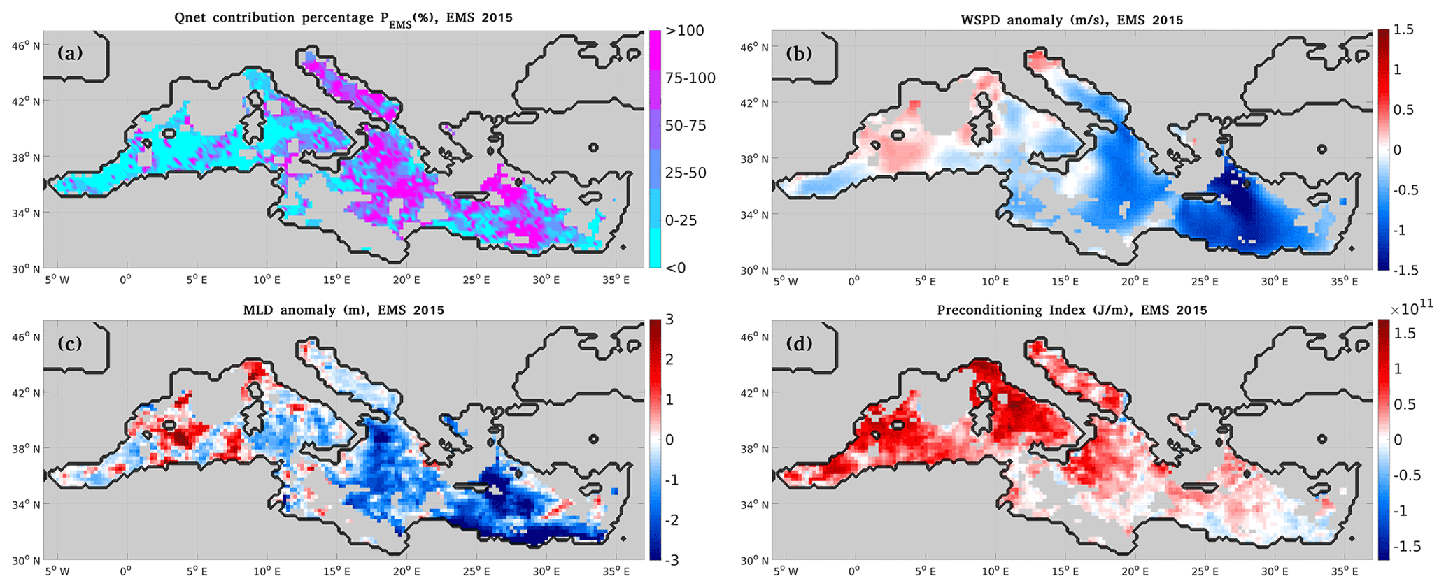
Figure 10 Panel (a) shows P_EMS metric values (%) for the contribution of Q_net to the formation of the extreme marine summer (EMS) 2015 (based on periods of positive cumulative SST anomalies and positive change in SST anomaly), (b–d) EMS anomalies of (b) wind speed at 10 m (m s⁻¹), (c) mixed layer depth (m), and (d) preconditioning index (J m⁻¹) for June 2015. EMS anomalies are computed with respect to their mean summer state based on 1950–2020 for wind speed and 1987–2019 for the mixed layer depth and the preconditioning index. Non-coloured sea grid points in the Mediterranean Sea stand for locations that did not experience summer 2015 as extreme.

Q_net appears to explain the EMS occurrence in most of the central and eastern basin (named as positive part from now on) (Fig. 10a). The Adriatic, Ionian, southern Aegean, and central Levantine seas present the highest P_EMS values, often exceeding 100 %. Few smaller areas, mostly scattered in the southern positive part, present negative P_EMS values. In such locations, other local processes are expected to surpass the “cooling” impact of the surface net heat balance and further drive the EMS SST anomalies.

Wind speed during this summer appears lower than usual in the entire positive part and particularly lower where P_EMS appears larger (Fig. 10a, b). Wind-forced LH flux anomalies are responsible here for the strong Q_net contribution, similarly to the mean EMS state in most Mediterranean areas. Consistently with the reduced winds, a decrease in MLD appears to further contribute to the EMS SST anomalies (Fig. 10b, c). In areas where Q_net corresponds to greater warming than the observed (P_EMS>100 %), such as in the southeastern Aegean and the central Ionian (where reduced vertical mixing additionally favours high SSTs), surface currents are highly expected to dump the residual warming.

In contrast, Q_net does not contribute to the EMS formation in several WMED areas (negative part) (Fig. 10a). This is related to the winds during this summer being stronger than usual in most of this area (Fig. 10b). Stronger winds in the negative part lead to (i) increased LH losses controlling the net heat flux signal (as typically occurs in EMSs) and (ii) increased vertical mixing as implied by the MLD anomalies being mostly positive in the negative part (Fig. 10b, c). On the other hand, the preconditioning index is clearly more pronounced here than in the positive part (Fig. 10d). Indeed, early-summer days (July 2015) present the largest SST anomalies within the season in this part of the basin. Further looking into the SST evolution throughout the year reveals positive SST anomalies (relevant to climatology) also during the precedent spring months (not shown). Therefore, the initial thermal state of the upper ocean in this part of the basin has worked in favour of the formation of this EMS.

Following 2015, other widely experienced EMSs such as 2003, 2012, and 2018 (in descending order by means of spatial extent) are examined (not shown). Results show that in case surface fluxes and stratification conditions do not contribute to surface warming, the preconditioning index presents an enhanced positive signal. Although not quantitative, the approach of using this index serves to diagnose whether there is a contributing role of this ocean memory-related factor in the formation of a summer as extreme. At the same time, it highlights the importance of considering in such studies the longer, compared to the atmosphere, ocean timescales.

4 Summary and conclusions

The Mediterranean Sea surface has undergone significant warming over the past decades, surpassing the warming observed in the global ocean and exhibiting even higher temperature trends during the summer season. The present study proposes the concept of extreme marine summers (EMSs) and investigates their characteristics in the MS in a climatological framework, using daily SST data from the ERA5 Reanalysis for the period 1950–2020. It explores the following: (i) the SST substructures during EMSs, (ii) the role of MHWs during EMSs, (iii) physical mechanisms related to the EMS formation focusing on the role of air–sea heat fluxes, and (iv) the impact of the SST multi-decadal variability in the studied EMS features.

EMSs identified in the MS over the study period display the largest mean seasonal SST anomalies in the western part of the basin, reaching up to 2.5 °C with respect to the local climatological mean summer values. In most of the basin, the seasonal SST anomalies are primarily formed due to the warmer summer days being anomalously warm. The main exception to this pattern is an area of the southern–central basin along the African coasts, where EMSs are formed mainly due to the colder summer days being warmer than normal. SST values in EMSs are organized closely following the climatological ranked daily SST variability. Locations where the warmest (coldest) part of the ranked daily SST distribution is more variable climatologically experience EMSs primarily due to the contribution of the warmest (coldest) part of the distribution.

Summer MHW events detected within 1950–2020 are more intense in northern MS regions, with the north-western basin exhibiting the highest MHW intensity, i.e. where the daily summer SSTs are more variable. MHWs in EMSs present greater intensity, duration, and frequency anomalies relative to mean summer MHW conditions in the northern parts of each sub-basin. In the rest of the basin (mainly in southern Mediterranean regions), MHWs contribute to EMSs by occurring more frequently and lasting longer, despite their intensity being lower than usual. In terms of temporal coverage of MHW conditions, a more pronounced role of MHWs during EMSs is found in the central and eastern Mediterranean, compared to the rest of the basin. Specifically, up to 55 % of locally detected MHW days over the period 1950–2020 fall within the four locally identified EMSs in these areas. Moreover, the vast majority of MHW days during EMSs (up to 95 %) take place within the warmest half of the SST distribution in the entire basin and especially in northern regions. Even in the south–central basin where the warmer than usual cool summer days are the most responsible for the elevated mean summer SST of EMSs, nearly 70 % of MHW days fall within the warmest part of the seasonal SST distribution.

Wind in EMSs appears weakened in the largest part of the basin and particularly in the Aegean and Levantine seas. These areas present the highest decreasing trends in wind magnitude over the past decades, in line with the observed suppression of LH losses. Reduced MLD in a great part of the basin during EMSs also suggests that highly stratified surface waters associated with concurrent low wind conditions are favouring conditions for the development of EMSs.

Surface heat flux anomalies in EMSs present strong spatial variability over the basin. They are primarily driven by LH fluxes in most areas, followed by SWR in the western and central basin and particularly in the Adriatic Sea. Positive Q_net anomalies are mainly formed by decreased LH loss from the sea surface and increased net SWR. The former is mostly met in the Aegean and Levantine seas as well as in the western part of the Gulf of Lions and the latter in the Adriatic Sea and is associated with reduced cloudiness during EMSs. Importantly, negative Q_net anomalies in EMSs are observed in a large part of the basin. This indicates that the elevated SST anomalies during EMSs in these areas are formed despite the non-favouring air–sea heat exchange, thus suggesting a key role of oceanic processes.

To quantify the driving role of Q_net in the EMS formation, a metric has been proposed based on the surface heat budget equation. This metric – expressed as a contribution percentage – focuses on selected SST changes, considered to be the most responsible for making a summer extreme. During these summer sub-periods, SST is kept above climatology through either (a) faster warming or (b) slower cooling compared to the corresponding climatological period.

Results show that EMSs are driven to a great extent by air–sea heat fluxes in the northern half of the MS. A latitudinal gradient is generally observed, with negative Q_net contribution percentages in the southern MS along the African coasts that progressively become positive while moving towards the north. Mixed layer shoaling due to decreased winds is a commonly observed complementary mechanism in areas where the examined SST anomalies are not entirely explained by surface heat fluxes. Q_net contribution percentages exceeding 100 % are also commonly met in the northern half of the basin (e.g. in Ligurian, Adriatic, North Aegean seas), meaning that additional processes (e.g. surface currents, vertical mixing) are expected to cancel the extra heating caused by surface fluxes.

Splitting the examined sub-periods in warming–cooling phases revealed that warming happening at a higher rate than usual is the main mechanism driving EMSs. Cooling at a lower rate than usual was found to be a process entirely explained by surface heat fluxes almost in the entire basin. However, such summer sub-periods correspond to a very small percentage (lower than 10 %) of the observed SST anomalies in EMSs. Therefore, this flux-driven cooling mechanism is not as important for the formation of an EMS as warming towards higher SST anomalies.

In the southernmost basin where air–sea heat exchanges were found to oppose the development of EMSs, oceanic processes, such as horizontal advection, are expected to be responsible for the high EMS SSTs. In these areas, the thermal deficit at the sea surface due to the non-favouring air–sea heat exchanges during EMSs is driven by enhanced LH loss (despite the diminished winds), associated with drier air masses during EMSs over the southern – compared to the northern – MS regions.

The role of upper-ocean preconditioning – potentially favouring the development of an EMS – is additionally examined by means of a proposed index. Preconditioning was diagnosed as a commonly contributing EMS formation factor. Decreased occurrence frequency of EMS preconditioning in the Alboran Sea and the Strait of Sicily suggests that it hardly develops in areas of intensified circulation. However, further investigation following these qualitative conclusions and assumptions is necessary towards a complete assessment of physical mechanisms related to EMSs in these areas.

Moreover, results suggest a link between MHW properties and surface heat fluxes in EMSs. The crucial role of Q_net found for the northernmost basin during EMSs is associated with its ability to drive MHWs of higher intensity. Consistently, surface heat fluxes were found to oppose the EMS formation in the southern MS where MHWs in EMSs are less intense, further supporting that Q_net modulates particularly the intensity of MHWs.

Finally, to gain insight into the impact of the SST multi-decadal variability in the studied EMS characteristics, a summer SST dataset free of multi-decadal trend was additionally produced. Removing the multi-decadal signal allowed us to explore EMS features beyond the long-term Mediterranean SST internal oscillation and climate change effect, in addition to the investigation of the summers actually experienced as extreme. To this end, the actual sea surface state – here represented by the ERA5 Reanalysis – was inter-compared with the detrended one. Results suggest the presence of a background SST anomaly field closely following the ranked daily SST variability pattern, on top of which the multi-decadal signal poses additional warming in the basin during EMSs. The dominant SST substructure revealed in the largest part of the basin (i.e. the warmest part of the SST distribution being responsible for the greatest part of the SST anomalies in EMSs) appears relatively independent of the multi-decadal trend. Importantly, in absence of multi-decadal variability, the contribution of Q_net to the EMS formation is found to be modulated by the LH component in the entire basin. Results suggest that, in addition to the fundamental role of LH flux, the observed Q_net during EMSs is further determined by the long-term variability of (i) the net SWR in the western and central basin and (ii) the wind-induced LH fluxes in the eastern basin.

Building upon this study, investigating SST substructures of extreme seasons in the MS using model ensemble data for present and future climate would strengthen the statistical confidence on the current results and point out differences among the observed and projected EMS conditions, respectively. Additionally, a broader assessment of physical mechanisms potentially contributing to the formation of local EMSs (e.g. horizontal advection, vertical mixing, water–heat transport through the Strait of Gibraltar and Strait of Sicily) would complement the current findings by providing insight into the relative role of oceanic factors. Finally, in the framework of building prediction tools, the potential use of an ocean heat content index, as an indicator for future anomalously warm seasons, could be a promising direction to explore.

Appendix A: Description of proposed metric

The proposed metric presented here is used to quantify the driving role of air–sea heat fluxes in the formation of EMSs. The metric focuses on summer sub-periods considered to be the most responsible for making a summer extreme. These are the periods where SST is kept above climatology through either (a) faster warming or (b) slower cooling compared to the corresponding climatological period. The metric is constructed according to the following steps:

Step 1. For each grid point, we split the 92 JAS summer days of each locally detected EMS in sequential warming and cooling phases.

Step 2. We isolate phases of positive cumulative SST anomaly:

$${\mathrm{SSTA}}_{\mathrm{cum}}>\mathrm{0},{\mathrm{SSTA}}_{\mathrm{cum}}=\sum _{t_{\mathrm{0}}}^{t_{\mathrm{1}}}({\mathrm{SST}}_t-{\mathrm{SST}}_{t_{\mathrm{clim}}}),$$

where SST_t and ${\mathrm{SST}}_{t_{\mathrm{clim}}}$ are the daily SST of day t and the corresponding climatological day t_clim, respectively. Indices t₀ and t₁ stand for the start and end day of each phase, respectively. This step isolates periods that contribute the most to the mean EMS SST.

Step 3. Among these phases, we further detect the ones where the observed SST evolves towards greater SST anomalies:

$$\begin{array}{c}{\displaystyle }\mathrm{\Delta }{\mathrm{SST}}_{\mathrm{obs}}^{\prime }>\mathrm{0},\\ {\displaystyle }\begin{array}{rl}\mathrm{\Delta }{\mathrm{SST}}_{\mathrm{obs}}^{\prime }& ={\mathrm{SST}}_{t_{\mathrm{1}}}^{\prime }-{\mathrm{SST}}_{t_{\mathrm{0}}}^{\prime }\\ & =({\mathrm{SST}}_{t_{\mathrm{1}}}-{\mathrm{SST}}_{t_{\mathrm{1}\mathrm{clim}}})-({\mathrm{SST}}_{t_{\mathrm{0}}}-{\mathrm{SST}}_{t_{\mathrm{0}\mathrm{clim}}})\end{array},\end{array}$$

where ${\mathrm{SST}}_{t_{\mathrm{0}}}^{\prime }$ and ${\mathrm{SST}}_{t_{\mathrm{1}}}^{\prime }$ are the daily SST anomalies at the start and the end day of each phase, respectively. During phases of $\mathrm{\Delta }{\mathrm{SST}}_{\mathrm{obs}}^{\prime }>\mathrm{0}$, SST either increases at a greater rate than usual (i.e. than climatologically) or decreases at a slower rate than usual.

To explain this criterion, let us suppose that a cooling phase evolves faster than climatologically ($\mathrm{\Delta }{{\mathrm{SST}}^{\prime }}_{\mathrm{obs}}<\mathrm{0}$). The criterion of step 2 (SSTA_cum>0) is potentially satisfied (depending on the initial conditions), but this phase will not be taken into account since SST changes towards lower anomalies. This is because even if Q_net entirely explains the observed cooling, such a positive contribution of Q_net to the observed SST decrease does not constitute a positive contribution in making this summer extreme (thus considered irrelevant to our purpose). In contrast, we are interested in examining the role of surface fluxes during phases when cooling occurs at a lower rate than usual, thus contributing to the development of an EMS through maintaining SST values above climatology. Similarly, we take into account phases during which warming occurs at a greater rate than usual, while a decelerated warming (with respect to climatology) falls out of our interest.

Step 4. For the selected phases (i.e. phases of both SSTA_cum>0 and $\mathrm{\Delta }{\mathrm{SST}}_{\mathrm{obs}}^{\prime }>\mathrm{0}$), we apply the surface heat budget equation using SST and Q_net anomalies:

$$\begin{array}{}\text{(A1)}& {\mathrm{SST}}_{t_{\mathrm{1}}}^{\prime }-{\mathrm{SST}}_{t_{\mathrm{0}}}^{\prime }=\underset{t_{\mathrm{0}}}{\overset{t_{\mathrm{1}}}{\int }}{\displaystyle \frac{Q_{\mathrm{net}}^{\prime }}{{\mathit{\rho }}_o{c}_{p}h}}\mathrm{d}t+R.\end{array}$$

The left-hand side of Eq. (A1) represents the observed change in SST anomaly relative to climatology, between days t₀ and t₁ (i.e. the term $\mathrm{\Delta }{\mathrm{SST}}_{\mathrm{obs}}^{\prime }$ computed at step 3). On the right-hand side of Eq. (A1), $Q_{\mathrm{net}}^{\prime }$ is the daily anomaly of Q_net relative to the mean climatological Q_net for this phase, i.e. $Q_{\mathrm{net}}^{\prime }=Q_t-\stackrel{\mathrm{‾}}{Q_{t_{\mathrm{clim}}}}$ , where $\stackrel{\mathrm{‾}}{Q_{t_{\mathrm{clim}}}}$ is the mean Q_net value within the climatological days t_0clim and t_1clim as implemented in Fewings and Brown (2019). The time integral of $Q_{\mathrm{net}}^{\prime }$ divided by the product of the constant values ρ (seawater density), c_p (specific heat capacity), and h (mixed layer thickness) represents the part of $\mathrm{\Delta }{\mathrm{SST}}_{\mathrm{obs}}^{\prime }$ that is attributed to $Q_{\mathrm{net}}^{\prime }$ during this phase (denoted by $\mathrm{\Delta }{\mathrm{SST}}_{Q_{\mathrm{net}}}$ from now on).

Accordingly, the second term of the right-hand side in Eq. (A1) stands for a change in SST anomaly due to non-heat flux (i.e. oceanic) factors affecting SST. These include the following: vertical mixing processes between the surface mixed layer and the rest of the water column, horizontal advection of SST, horizontal eddy heat fluxes, and radiative heat loss due to SWR penetration below the mixed layer depth.

Step 5. We compute the percentage of Q_net contribution for each phase N:

$$P\left(N\right)={\displaystyle \frac{\mathrm{\Delta }{\mathrm{SST}}_{Q_{\mathrm{net}}}\left(N\right)}{\mathrm{\Delta }{\mathrm{SST}}_{\mathrm{obs}}^{\prime }\left(N\right)}}\cdot \mathrm{100}\mathit{\%}.$$

Step 6. To obtain a mean percentage for the entire summer, we weight the contribution percentage of each phase according to the phase's SSTA_cum. The weighting coefficient of each phase (N) of the selected phases (NS) may be written as follows:

$$\begin{array}{rl}W\left(N\right)& ={\displaystyle \frac{{\mathrm{SSTA}}_{\mathrm{cum}}\left(N\right)}{{\mathrm{SSTA}}_{{\mathrm{cum}}_{\mathrm{ALL}}}}}\\ & ={\displaystyle \frac{\sum _{t_{\mathrm{0}}}^{t_{\mathrm{1}}}({\mathrm{SST}}_t\left(N\right)-{\mathrm{SST}}_{t_{\mathrm{clim}}})}{\sum _{N=\mathrm{1}}^{\mathrm{NS}}\sum _{t_{\mathrm{0}}}^{t_{\mathrm{1}}}({\mathrm{SST}}_t\left(N\right)-{\mathrm{SST}}_{t_{\mathrm{clim}}})}},\\ & \sum _{N=\mathrm{1}}^{\mathrm{NS}}W\left(N\right)=\mathrm{1}.\end{array}$$

The metric value (P_i) for the Q_net contribution to each EMS (i) is then

$$P_i=\sum _{N=\mathrm{1}}^{\mathrm{NS}}P\left(N\right)\cdot W\left(N\right),$$

while the final metric for the mean EMS state, being the mean (among the four EMSs) of the above percentage, is

$$P_{\mathrm{EMS}}={\displaystyle \frac{\mathrm{1}}{\mathrm{4}}}\sum _{i=\mathrm{1}}^{\mathrm{4}}{P}_i.$$

This weighting approach promotes phases of higher SSTA_cum considering their higher impact on the mean EMS SST. Nevertheless, sensitivity tests using different scaling (e.g. based on phase duration) present very similar results, suggesting a negligible sensitivity of the metric to these choices for averaging.

Step 7. As an additional task, we repeat steps 3 to 5 separately for the warming and cooling phases (subscripts w and c, respectively). Then, analogously to step 6, the weighting coefficient of each (N) phase for the selected warming (NS_w) and cooling (NS_c) phases is

$$\begin{array}{rl}{W}_{\mathrm{w}\mathrm{|}\mathrm{c}}\left(N\right)& ={\displaystyle \frac{{\mathrm{SSTA}}_{\mathrm{cum},\mathrm{w}\mathrm{|}\mathrm{c}}\left(N\right)}{{\mathrm{SSTA}}_{\mathrm{cum},\mathrm{w}\mathrm{|}{\mathrm{c}}_{\mathrm{ALL}}}}}\\ & ={\displaystyle \frac{\sum _{t_{\mathrm{0}}}^{t_{\mathrm{1}}}({\mathrm{SST}}_t\left(N\right)-{\mathrm{SST}}_{t_{\mathrm{clim}}})}{\sum _{N=\mathrm{1}}^{{\mathrm{NS}}_{\mathrm{W}\mathrm{|}\mathrm{C}}}\sum _{t_{\mathrm{0}}}^{t_{\mathrm{1}}}({\mathrm{SST}}_t\left(N\right)-{\mathrm{SST}}_{t_{\mathrm{clim}}})}},\\ & \sum _{N=\mathrm{1}}^{{\mathrm{NS}}_{\mathrm{W}\mathrm{|}\mathrm{C}}}{W}_{\mathrm{w}\mathrm{|}\mathrm{c}}\left(N\right)=\mathrm{1}.\end{array}$$

The metric value for the Q_net contribution in the selected warming–cooling phases, for each EMS (i), is

$$P_{i_{\mathrm{w}\mathrm{|}\mathrm{c}}}=\sum _{N=\mathrm{1}}^{{\mathrm{NS}}_{\mathrm{W}\mathrm{|}\mathrm{C}}}P\left(N\right)\cdot W_{\mathrm{w}\mathrm{|}\mathrm{c}}\left(N\right),$$

while the final metric, being the mean (among the four EMSs) of the above percentage for the selected warming–cooling phases, is

$$P_{{\mathrm{EMS}}_{\mathrm{w}\mathrm{|}\mathrm{c}}}={\displaystyle \frac{\mathrm{1}}{\mathrm{4}}}\sum _{i=\mathrm{1}}^{\mathrm{4}}{P}_{i_{\mathrm{w}\mathrm{|}\mathrm{c}}}.$$

Appendix B: Additional figures

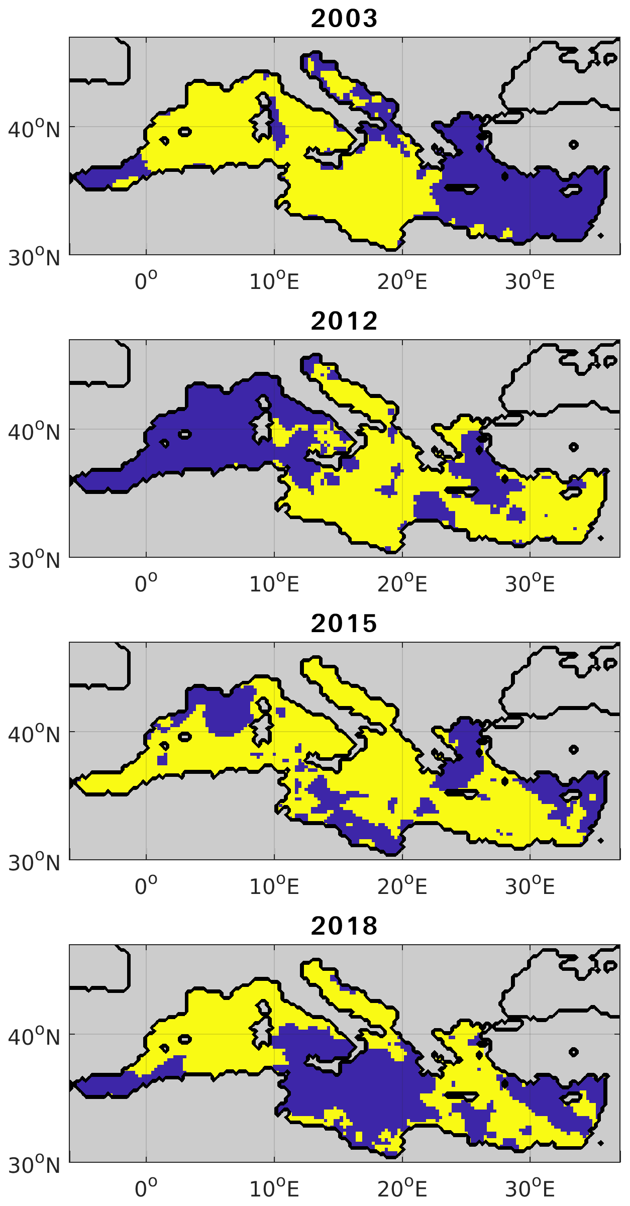
Figure B1 EMSs concentrating more than 50 % of the Mediterranean Sea grid points: 2003, 2012, 2015, and 2018 (from top to bottom, respectively). Yellow stands for areas experiencing EMS conditions and blue for non-EMS conditions.

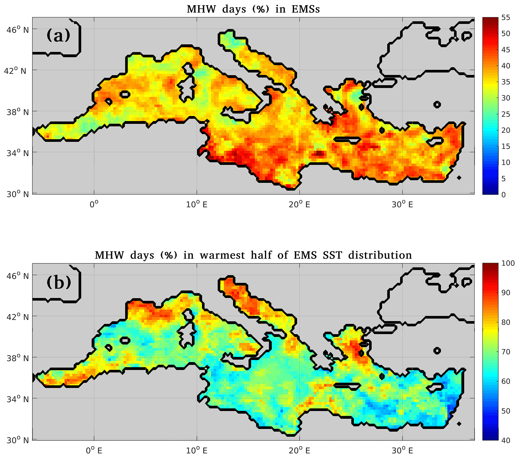
Figure B2 (a) Percentage of summer MHW days falling within EMSs, with respect to the total count of summer MHW days within 1950–2020. (b) Percentage of summer MHW days falling within the warmest half of the SST distribution during EMSs, with respect to the total count of summer MHW days within EMSs (the corresponding percentage for the coldest half of the SST distribution is the remaining percentage).

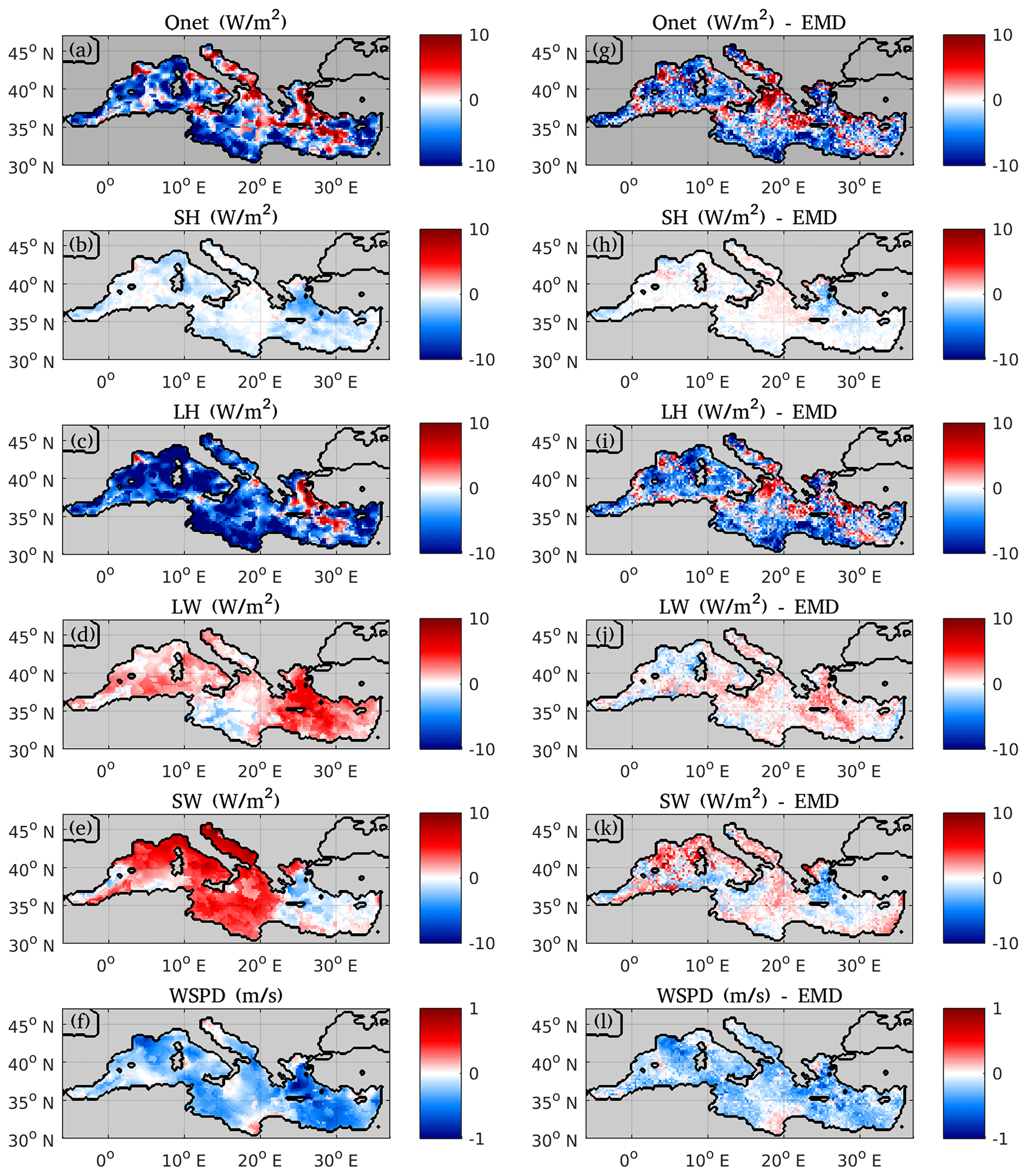
Figure B3 (a–f) Extreme marine summer (EMS) anomalies of surface fluxes and wind speed at 10 m with respect to the mean summer state (1950–2020). (a) Q_net, (b) sensible heat flux, (c) latent heat flux, (d) net long-wave radiation, (e) net short-wave radiation, and (f) wind speed. (g–l) Same as (a)–(f) but using detrended data. Downwards fluxes have been considered as positive, so positive EMS anomaly values correspond to either heat gain or reduced loss from the sea surface.

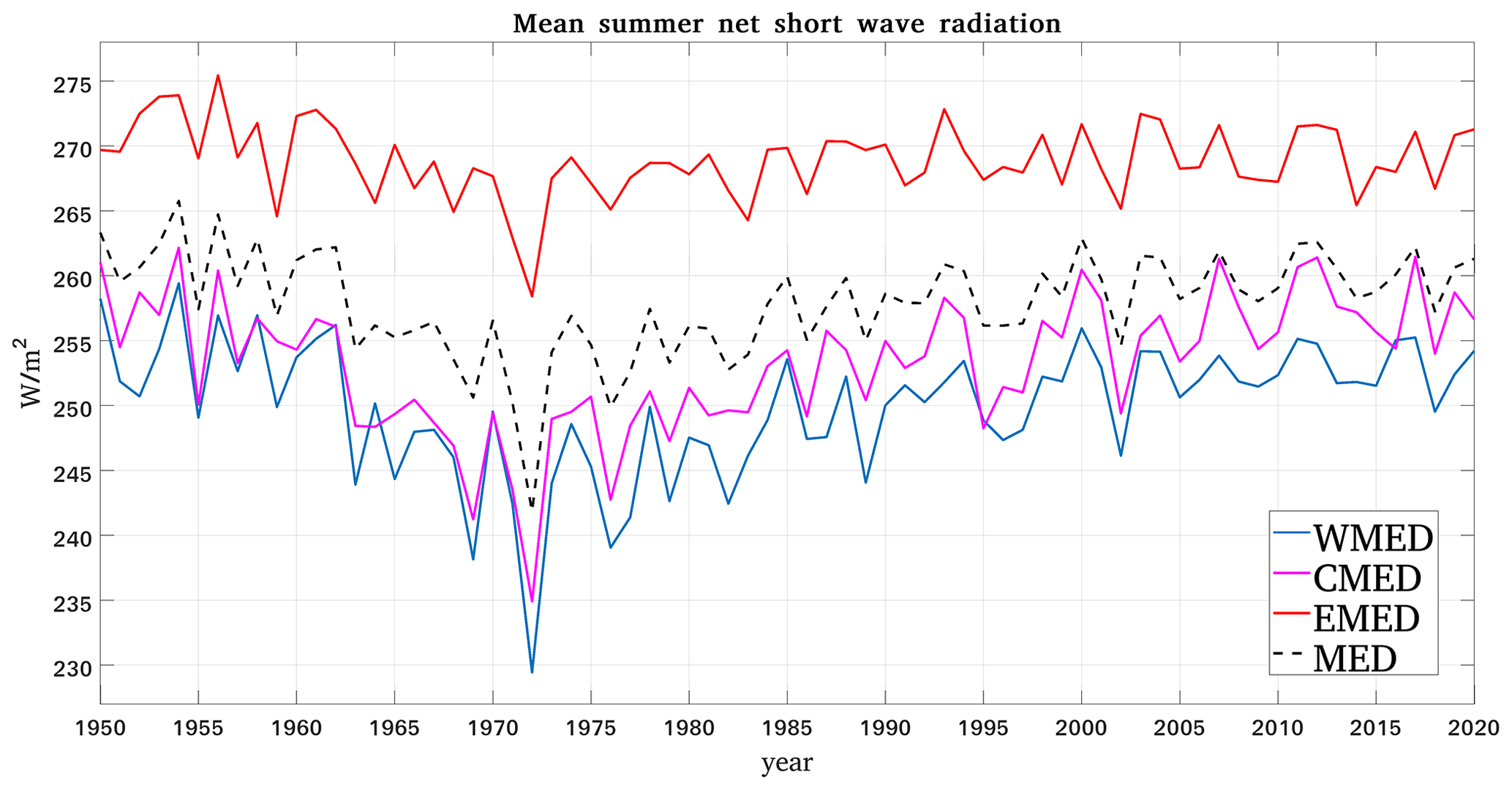
Figure B4 ERA5 mean summer net short-wave radiation (W m⁻²) in the Mediterranean Sea (1950–2020) for the entire basin (dashed black line) and for the western (extending from the Strait of Gibraltar to the Strait of Sicily; blue line), central (Strait of Sicily up to 22° E; purple line) and eastern (22° E eastwards; red line) sub-basins.

Figure B5 Extreme marine summer anomalies (relative to the mean summer state based on the period 1950–2020) for the (a) ERA5 total cloud cover and (b) ERA5 specific humidity (kg kg⁻¹).