Internal tides off the Amazon shelf – Part 1: The importance of the structuring of ocean temperature during two contrasted seasons

The impact of internal and barotropic tides on the vertical and horizontal temperature structure off the Amazon River was investigated during two highly contrasted seasons (AMJ: April–May–June; ASO: August–September–October) over a 3-year period from 2013 to 2015. Twin regional simulations, with and without tides, were used to highlight the general effect of tides. The findings reveal that tides have a cooling effect on the ocean from the surface (∼ 0.3 ^∘C) to above the thermocline (∼ 1.2 ^∘C), while warming it up below the thermocline (∼ 1.2 ^∘C). The heat budget analysis indicates that the vertical mixing is the dominant process driving temperature variations within the mixed layer, while it is associated with both horizontal and vertical advection to explain temperature variations below. The increased mixing in the simulations including tides is attributed to breaking of internal tides (ITs) on their generation sites over the shelf break and offshore along their propagation pathways. Over the shelf, mixing is driven by the dissipation of the barotropic tides. In addition, the vertical terms of the heat budget equation exhibit wavelength patterns typical of mode-1 IT. The study highlights the key role of tides and particularly how IT-related vertical mixing shapes the ocean temperature off the Amazon. Furthermore, we found that tides impact the interactions between the upper ocean interface and the overlying atmosphere. They contribute significantly to increasing the net heat flux between the atmosphere and the ocean, with a notable seasonal variation from 33.2 % in AMJ to 7.4 % in ASO seasons. This emphasizes the critical role of tidal dynamics in understanding regional-scale climate.

1 Introduction

In the ocean, many processes depend on temperature. These processes include water mass formation (Swift and Aagaard, 1981; Lascaratos, 1993; Speer et al., 1995); the transport and mixing of tracers; exchanges with other biosphere compartments (Archer et al., 2004; Rosenthal et al., 1997); and, most importantly, surface heat exchange at the interface with the atmosphere (Clayson and Bogdanoff, 2013; Mei et al., 2015), which significantly influence the climate (Li et al., 2006; Collins et al., 2010). The oceanic thermal structure can be modified at various spatial and temporal scales through external processes such as solar radiation; heat exchanges with the atmosphere; winds; precipitation; freshwater inputs from rivers; and internal processes including mass transport by currents and eddies (e.g., Aguedjou et al., 2021), mixing by turbulent diffusion (Kunze et al., 2012), and the dissipation of internal waves (Barton et al., 2001; Smith et al., 2004; Salamena et al., 2021). Additionally, bottom friction of barotropic tidal currents can lead to intensified mixing, particularly in shallow-water conditions over a shelf (see Lambeck and Runcorn, 1977; Le Provost and Lyard, 1997), and significantly modify ocean temperature in surface layers (Li et al., 2020).

The barotropic tides, also called external tides, serve as the primary source for generating internal waves. When barotropic tides interact with sharp topography such as ridges, sea mounts, and shelf breaks in a stratified ocean, they generate internal tides (IT) that propagate and dissipate in the ocean interior causing diapycnal mixing (Baines, 1982; Munk and Wunsch, 1998; Egbert and Ray, 2000). Several observational and modeling studies have demonstrated that this dissipation occurs at the generation sites, through reflection at the ocean bottom, or near the surface when the energy rays interact with the pycnocline (among others: Laurent and Garrett, 2002; Sharples et al., 2007, 2009; Koch-Larrouy et al., 2015; Nugroho et al., 2018; Whalen et al., 2012). ITs also dissipate or lose energy through wave–wave interactions or when they interact with mesoscale or fine-scale structures (Vlasenko and Stashchuk, 2006; Dunphy and Lamb, 2014).

The role of ITs in shaping the ocean's thermal structure has garnered increasing interest and has been the focus of numerous studies in recent years. In the shallow shelf surface waters of Hawaii, Smith et al. (2016) reported that IT can induce surface cooling ranging from 1–5 ^∘C. Similarly, in the Indonesian region, studies by Koch-Larrouy et al. (2007, 2008), Nagai and Hibiya (2015), and Nugroho et al. (2018) found that ITs lead to an average surface cooling of 0.5 ^∘C, which subsequently reduces local atmospheric convection and results in a 20 % decrease in precipitation. Therefore, ITs play a significant role in the regional climate dynamics (Koch-Larrouy et al., 2010; Sprintall et al., 2014, 2019). Furthermore, Jithin and Francis (2020) demonstrated that ITs can influence the temperature of deep waters (>1600 m) in the Andaman Sea, resulting in a warming effect of about 1–2 ^∘C. However, the impact of IT on temperature off the Amazon plateau is still not well understood.

Our study focuses on the oceanic region of northern Brazil off the Amazon River. This region experiences variations in wind patterns and hence the position of the Intertropical Convergence Zone (ITCZ) throughout the year. These variations directly impact the discharge of the Amazon River, oceanic circulation, eddy kinetic energy (EKE), and stratification (Muller-Karger et al., 1988; Johns et al., 1990; Xie and Carton, 2004). Consequently, two contrasted seasons emerge: April–May–June (AMJ) and August–September–October (ASO). The AMJ (vs. ASO) season features an increasing (vs. decreasing) river discharge, there is a stronger (vs. weaker) and shallower (vs. deeper) pycnocline, while the North Brazilian Current (NBC) and EKE are weaker (vs. stronger) (Aguedjou et al., 2019; Tchilibou et al., 2022). During AMJ season, NBC forms a weak equatorial retroflection that contributes to the Equatorial Under Current. In the ASO season, when NBC strengthens, it forms a stronger retroflection in the northwest, which feeds the North Equatorial Counter Current and transports water masses eastwards into the tropical Atlantic. This intensified retroflection gives rise to large anticyclonic eddies called NBC Rings, which can exceed 450 km in diameter (Didden and Schott, 1993; Richardson et al., 1994; Garzoli et al., 2003). These eddies play a role in transporting water masses towards the Northern Hemisphere (Bourles et al., 1999; Johns et al., 1998; Schott et al., 2003).

In this region, IT are generated at the sharp shelf break, where the depth decreases from 200–2000 m over a few tens of kilometers (Fig. 1). Six main sites (A to F) have been identified, with the most intense sites, A and B, located in the southern part of the region (Fig. 1; Magalhaes et al., 2016; Tchilibou et al., 2022). Previous studies have indicated that the propagation of IT in this region is modulated by seasonal variation in currents (Magalhaes et al., 2016; Lentini et al., 2016; Tchilibou et al., 2022). Moreover, changes in stratification throughout different seasons affect the activity of internal tides. In AMJ (vs. ASO) season, there is a stronger (vs. smaller) energy conversion and a stronger (vs. smaller) local dissipation of IT energy (Barbot et al., 2021; Tchilibou et al., 2022). The interaction between the weaker (vs. stronger) background circulation and IT results in fewer (vs. more) incoherent or non-stationary internal tides (Tchilibou et al., 2022).

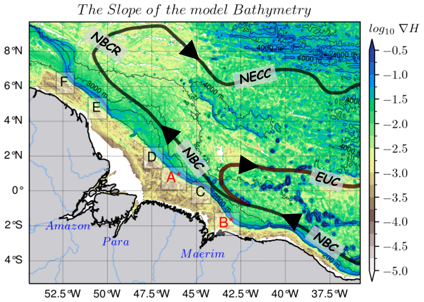
Figure 1 The horizontal gradient of the model's bathymetry (∇H) with internal tide generation sites (A^*, B^*, C, D, E, and F) along the high slope of the shelf break (blue shading), with the two main sites being A^* and B^* (in red), as reported in Magalhaes et al. (2016) and Tchilibou et al. (2022). Solid bold lines represent a schematic view of the circulation (as described by Didden and Schott, 1993; Richardson et al., 1994; Johns et al., 1998; Bourles et al., 1999; Schott et al., 2003; Garzoli et al., 2003) with the NBC, NBC Rings, and North Equatorial Counter Current tracks in black and the Equatorial Under Current track in brown red. Thin black contours are 200, 2000, 3000, and 4000 m isobaths from the model bathymetry.

During the ASO season, cold water with temperature below 27.6 ^∘C, associated with the western extension of the Atlantic Cold Tongue (ACT), flows into the region from the south and runs along the edge of the continental shelf up to 3^∘ N, forming a cold cell known as seasonal upwelling (Lentz and Limeburner, 1995; Neto and da Silva, 2014). Based on in situ observations, the latter suggests that this cooling is backed by the vertical advection triggered by the NBC. Alternatively, Ruault et al. (2020) conducted a modeling study, comparing simulations with and without tides, and demonstrated that the inclusion of tides resulted in a more realistic cooling effect on this upwelling. However, it remains unclear whether the cooling is a result of mixing on the shelf caused by barotropic tides or mixing caused by baroclinic tides at their generation sites and propagation pathways.

To answer the previous questions, we use a high-resolution model ($\mathrm{1}/\mathrm{36}$^∘) with and without explicit tidal forcing and a satellite sea surface temperature (SST) product. Our aim is to examine the impact of tides on the temperature structure and quantify the associated processes for the two contrasted seasons (AMJ and ASO) described above. Section 2 provides a description of the SST product, our model, and the methods used. The validation of tidal characteristics and the temperature are presented in Sect. 3. Section 4 focuses on the analysis of the impacts of tides on the temperature structure and the associated processes, as well as the influence of tides on heat exchange at the atmosphere–ocean interface. The discussion and summary of the obtained results are presented in Sects. 5 and 6, respectively.

2 Data and methods

2.1 Satellite data: TMI SST

This dataset is derived from Tropical Rainfall Measurement Mission (TRMM), which performs measurements using an onboard TRMM Microwave Imager (TMI). The microwaves can penetrate clouds and are therefore crucially important for data acquisition in low latitude regions, cloudy covered during long periods of raining seasons. We use TMI data product v7.1, which is the most recent version of TMI SST. It contains a daily mean of SST with a 0.25^∘ × 0.25^∘ grid resolution (∼25 km). This SST is obtained through inter-calibration of TMI data with other microwave radiometers. The full description of TMI SST and its inter-calibration algorithm are detailed in Wentz (2015).

2.2 The NEMO model: AMAZON36 configuration

The numerical model used in this study is the Nucleus for European Modeling of the Ocean (NEMO v4.0.2, Madec et al., 2019). The specific configuration designed for this study is called AMAZON36 and covers the western tropical Atlantic region from the Amazon River mouth to the open ocean. Other configurations in this region either have a coarse grid ($\mathrm{1}/\mathrm{4}$^∘, Hernandez et al., 2016) or, when the grid is fine ($\mathrm{1}/\mathrm{36}$^∘), do not extend far enough eastwards and exclude most of site B (Ruault et al., 2020). The current AMAZON36 configuration overcomes these limitations. The grid resolution is $\mathrm{1}/\mathrm{36}$^∘ and the domain spans between 54.7–35.3^∘ W and 5.5^∘ S–10^∘ N (Fig. 1). In this way, we capture the internal tides radiating from all the generating sites on the Brazilian shelf break. The vertical grid consists of 75 vertically fixed z-coordinate levels, with a narrower grid refinement near the surface, comprising 23 levels in the first 100 m, whereas cell thickness reaches 160 m near the bottom. The horizontal and vertical resolutions of the grid are therefore fine enough to resolve low-mode IT. This grid resolution has been previously used for a similar purpose in this region (e.g., Tchilibou et al., 2022).

A third-order upstream biased scheme (UP3) with built-in diffusion is used for momentum advection, while tracer advection relies on a second-order flux-corrected transport (FCT) scheme (Zalesak, 1979). A Laplacian isopycnal diffusion with a constant coefficient of 20 m² s⁻¹ is used for tracers. The temporal integration is achieved thanks to a leapfrog scheme combined with an Asselin filter to damp numerical modes, with a baroclinic time step of 150 s. The k-ε turbulent closure scheme is used for vertical diffusion. Bottom friction is quadratic with a bottom drag coefficient of $\mathrm{2.5}\times {\mathrm{10}}^{-\mathrm{3}}$, while lateral wall free-slip boundary conditions are prescribed. A time-splitting technique is used to resolve the free surface, with the barotropic part of the dynamical equations integrated explicitly.

We use the 2020 release of the General Bathymetric Chart of the Oceans, which has been interpolated onto the model's horizontal grid, with the minimal depth set to 12.8 m. The model is forced at the surface by the ERA-5 atmospheric reanalysis (Hersbach et al., 2020). River runoff is based on monthly means from hydrology simulation of the Interaction Sol-Biosphère-Atmosphère model (ISBA, https://www.umr-cnrm.fr/spip.php?article146&lang=en, last access: 15 November 2020) and are prescribed as surface mass sources with null salinity. We use 90 % of ISBA runoff based on a comparison with the HYBAM runoff time series (http://www.ore-hybam.org, last access: 15 November 2020). The model is forced at its open boundaries by the 15 major tidal constituents (M₂, S₂, N₂, K₂, 2N₂, MU₂, NU₂, L₂, T₂, K₁, O₁, Q₁, P₁, S₁, and M₄) and barotropic currents derived from the FES2014 atlas (Lyard et al., 2021). In addition, we prescribe to the open boundaries the temperature, salinity, sea level, current velocity, and derived baroclinic velocity from the recent MERCATOR-GLORYS12 v1 assimilation data (Lellouche et al., 2018).

The simulations were initialized on 1 January 2005 and ran for 11 years until December 2015. It was found that the model achieved a seasonal cycle equilibrium after 2 years. However, for this study, our focus lies on a 3-year period from January 2013 to December 2015. To highlight the influence of tides on the temperature structure, we use a twin model configuration without tidal forcing.

2.3 Methods

2.3.1 Tide energy budget

We follow Kelly et al. (2010) to separate barotropic and baroclinic tide constituents. There is no separation following vertical modes, then we analyze the total energy for all the resolved propagation modes for a given tidal frequency. Note that the barotropic–baroclinic tide separation is performed directly by the model for better accuracy. We have only analyzed the M₂ harmonic, which is the major tidal constituent in this region (Prestes et al., 2018; Fassoni-Andrade et al., 2023), representing ∼70 % of the tidal energy (Beardsley et al., 1995; Gabioux et al., 2005).

The energy budget equations of barotropic and baroclinic tides are obtained assuming that the energy tendency, the nonlinear advection, and the forcing terms are small (Wang et al., 2016). The remaining equations are reduced to the balance between the energy dissipation, the divergence of the energy flux, and the energy conversion from barotropic to baroclinic (e.g., Buijsman et al., 2017; Tchilibou et al., 2018, 2020; Jithin and Francis, 2020; Peng et al., 2021):

$$\begin{array}{}\text{(1)}& {\displaystyle }{D}_{\mathrm{bt}}+{\mathrm{\nabla }}_h\cdot F_{\mathrm{bt}}+C\approx \mathrm{0},\text{(2)}& {\displaystyle }{D}_{\mathrm{bc}}+{\mathrm{\nabla }}_h\cdot F_{\mathrm{bc}}-C\approx \mathrm{0},\end{array}$$

where bt and bc indicate the barotropic and baroclinic terms, respectively; D is the depth-integrated energy dissipation, which can be understood as a proxy of the real dissipation since D may encompass the energy loss of nonlinear terms and/or numerical dissipation (see Nugroho et al., 2018); ∇_h⋅F represents the divergence of the depth-integrated energy flux; and C is the depth-integrated barotropic-to-baroclinic energy conversion, i.e., the amount of incoming barotropic energy converted into internal tides energy over the steep topography:

$$\begin{array}{}\text{(3)}& {\displaystyle }C=\langle \mathrm{\nabla }H\cdot U_{\mathrm{bt}}{P}_{\mathrm{bc}}^{*}\rangle ,\text{(4)}& {\displaystyle }{F}_{\mathrm{bt}}=\langle U_{\mathrm{bt}}{P}_{\mathrm{bt}}\rangle ,\text{(5)}& {\displaystyle }{F}_{\mathrm{bc}}=\underset{H}{\overset{\mathit{\eta }}{\int }}\langle U_{\mathrm{bc}}{P}_{\mathrm{bc}}\rangle d_z,\end{array}$$

where the angle bracket 〈⋅〉 denotes the average over a tidal period, ∇H is the slope of the bathymetry, U is the current velocity, $P_{\mathrm{bc}}^{*}$ is the baroclinic pressure perturbation at the bottom, H is the bottom depth, η is the surface elevation, P is the pressure, and F is the energy flux that indicates the path of tides.

2.3.2 The 3-D heat budget equation for temperature

The three-dimensional temperature budget was computed online and further analyzed. It is the balance between the total temperature trend and the sum of the temperature advection, diffusion and solar radiative and non-solar radiative fluxes (e.g., Jouanno et al., 2011; Hernandez et al., 2017). The three-dimensional heat budget equation for temperature is expressed as follows:

$$\begin{array}{}\text{(6)}& \begin{array}{rl}{\partial }_{t}T& =\underset{\mathrm{ADV}}{\underbrace{-u{\partial }_{x}T-v{\partial }_{y}T-w{\partial }_{z}T}}+\mathrm{LDF}\\ & -\underset{\mathrm{ZDF}}{\underbrace{{\partial }_z\left(K_z{\partial }_{z}T\right)}}+\mathrm{Forcing}+\mathrm{Asselin}\end{array}\end{array}$$

here T is the model potential temperature, ($u,v,w$) are the velocity components in the ($x,y,z$) (eastward, northward, and upward, respectively) directions, and ADV is the 3-D tendency term from the advection routine of the NEMO code (left to right: zonal, meridional, and vertical terms). Note that in our model ADV includes some diffusivity of the temperature due to numerical dissipation of the FCT advection scheme (Zalesak, 1979) in contrast to some non-diffusive advection schemes like in Leclair and Madec (2009). In previous studies, at lower resolutions ($\mathrm{1}/\mathrm{4}$^∘) this mixing has been quantified to be responsible for 30 % of the dissipation as part of the high-frequency effect of the diffusion (Koch-Larrouy et al., 2008). We expect here at $\mathrm{1}/\mathrm{36}$^∘ resolution that this effect will be smaller but still non-negligible. Note that explicit separation of this effect is beyond the scope of our study. Furthermore, tides are primarily linear in surface water; however, nonlinear effects intensify due to bottom friction for barotropic tides or as a result of IT breaking. Consequently, we anticipate a corresponding increase in ADV. ZDF denotes the vertical diffusion; LDF is the lateral diffusion; forcing is the sum of tendency of temperature due to penetrative solar radiation, which includes a vertical decaying structure and the non-solar heat flux (sum of the latent, sensible, and net infrared fluxes) at the surface layer; and Asselin corresponds to the numerical diffusion for the temperature.

3 Model validation

In this section, we assess the quality of our simulations by verifying whether they are in good agreement with the observations and other reference data. Firstly, for the barotropic and baroclinic characteristics of the M₂ tides for the year 2015 and secondly for the temperature from 2013 to 2015.

3.1 M₂ tides in the model

We initially examined the barotropic sea surface height (SSH), and there is a good agreement in both amplitude and phase between FES2014 and the model (Fig. 2a and b, respectively). However, near the coast, few differences in amplitude are observed. The model's SSH amplitude is lower (∼50 cm) north of the mouth of the Amazon, while it overestimates the amplitude by ∼20 and ∼40 cm, respectively, shoreward and on the southern part of the mouth. These biases are of a similar magnitude as those reported in Ruault et al. (2020). The flux of the barotropic tidal energy flowing inshore is depicted in Fig. 2c and d for FES2014 and the model, respectively. A portion of this energy is converted into baroclinic tidal energy over the steep slope of the bathymetry. We compared the depth-integrated barotropic-to-baroclinic energy conversion rate (C) between FES2014 and the model, Fig. 2c and d, respectively. The model successfully reproduces the same conversion patterns of FES2014 over the slope but less so offshore between 42–35^∘ W and 7–10^∘ N. As a result, our model underestimates C overall by approximately 30 %. Niwa and Hibiya (2011) demonstrated that C increases with higher bathymetry resolution. This indicates that there is more conversion with the FES2014 grid (∼1.5 km) compared to our grid (∼3 km).

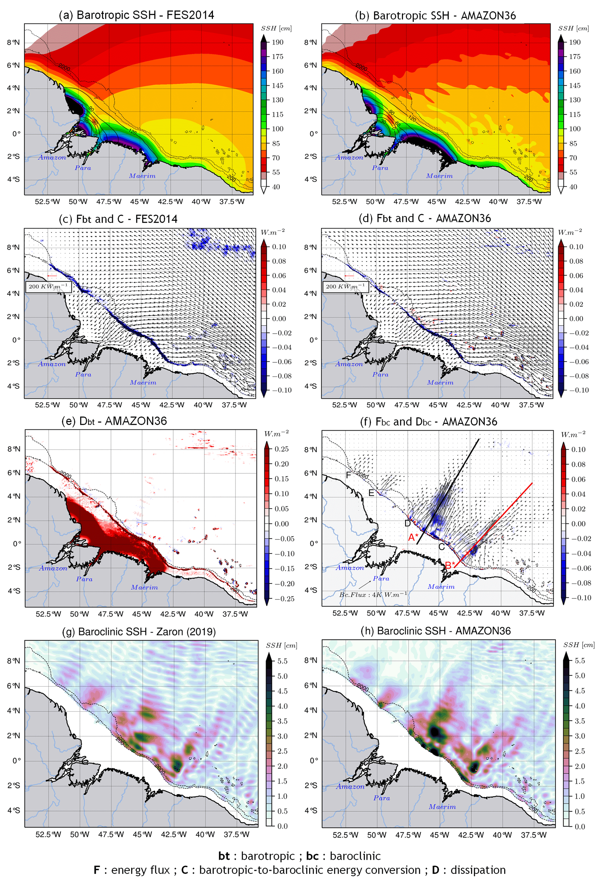
Figure 2 Characteristics of M₂ coherent tides. Barotropic SSH amplitude (color shading) and its phase (solid contours) for (a) FES2014 and (b) the model, barotropic energy flux (black arrows) with the energy conversion rate (color shading) for (c) FES2014 and (d) the model, (e) the model depth-integrated barotropic energy dissipation, (f) the model depth-integrated baroclinic energy flux (black arrows) and the depth-integrated baroclinic energy dissipation (color shading) with transect lines along IT trajectories A^* (black) and B^* (red), and the baroclinic SSH amplitude from (g) Zaron (2019) and (h) the model. Data from the model are the mean value over the year 2015. For all panels, dashed black contours represent the 200 and 2000 m isobaths of the model bathymetry.

Another portion of the barotropic energy is dissipated on the shelf through bottom friction, leading to mixing from the bottom (Beardsley et al., 1995; Gabioux et al., 2005; Bessières, 2007; Fontes et al., 2008). Most of the dissipation of barotropic energy (D_bt) occurs in the middle and inner shelf between 3^∘ S–4^∘ N with a mean value of about 0.25 W m⁻² (Fig. 2e). The location of this dissipation aligns well with previous studies of Beardsley et al. (1995) and Bessières (2007). The remaining barotropic energy propagates over hundreds of kilometers into the estuarine systems of this region (Kosuth et al., 2009; Fassoni-Andrade et al., 2023).

The energy flux of ITs (F_bc) indicates that they propagate from the slope towards the open ocean (Fig. 2f). F_bc indicates the existence of six main sites of IT generation on the slope, with sites A and B being particularly significant in terms of their higher and greatly extended energy flux, in good agreement with previous studies (Magalhaes et al., 2016; Barbot et al., 2021 and Tchilibou et al., 2022). From these two main sites, ITs spread over nearly 1000 km and dissipate their energy. The model's depth-integrated internal tides energy dissipation (D_bc) is at least 2 times weaker than barotropic energy dissipation, with a mean value of 0.1 W m⁻² (Fig. 2f). Approximately 30 % of IT energy is dissipated locally over generation sites (not shown), consistent with the findings of Tchilibou et al. (2022). The remaining portion is dissipated offshore along the propagation path. This offshore dissipation is more extended along path A, ∼300 km from the slope, with two beams spaced by an average distance of 120–150 km corresponding to mode-1 wavelength. On the other hand, there is less offshore dissipation along path B, occurring around 100–200 km from the slope (Fig. 2f).

Another important characteristic of IT is their SSH imprints along the propagation pathway. The estimate of this signature deduced from the altimeter tracks (Fig. 2g) produced by Zaron (2019) is compared with our model (Fig. 2h), with the shelf masked over 150 m depth. Our model shows good agreement with this product, albeit with a slight overestimation of about ∼1.5 cm on the SSH amplitude maxima. It is worth noting that the model's baroclinic SSH amplitude is an average over the year 2015, while the satellite estimate is an average over a longer period of about 20 years. The longer period of the satellite estimate may introduce greater variability in the altimeter tracks, potentially reducing the amplitude of the estimates and explaining the slight differences with the model in the positioning and amplitude of the maxima.

3.2 Temperature validation

Figure 3 shows the mean SST over the entire 2013–2015 period for TMI (Fig. 3a), the tidal simulations (Fig. 3b), and the non-tidal simulations (Fig. 3c). We obtain the bias between TMI SST and the two simulations by linear interpolation of the simulations data on the observation grid. The simulations with tides accurately reproduce the spatial distribution of the observations, as indicated by the weak bias ($<\pm \mathrm{0.1}$ ^∘C) with TMI SST. This is particularly evident for the cooling on the shelf around 47.5^∘ W and to the southeast between 40–35^∘ W and 2^∘ S–2^∘ N (Fig. 3d). In contrast, the non-tidal simulations exhibit a warm bias of about 0.3 ^∘C in this cooling region (Fig. 3e). To the northeast, between 50–54^∘ W and 3–8^∘ N in the Amazon plume, the SST of the non-tidal simulations is in better agreement with the observations, while the SST of the tidal simulations is about 0.6 ^∘C cooler than TMI SST (Fig. 3d). This bias is consistent with other models that include tides in this northern zone (e.g., Hernandez et al., 2016, 2017; Gévaudan et al., 2022). Far offshore, between 50–40^∘ W and 6–10^∘ N, both simulations exhibit a negative bias of about 0.2–0.3 ^∘C (Fig. 3d–e). We averaged the observations and interpolated simulation data within the dashed box (Fig. 3a–c), with a depth of less than 200 m masked. This location of the boxes comprises IT generation sites and part of their pathways. We then computed the seasonal cycle of the three products (Fig. 3f). The tidal and non-tidal simulations accurately reproduce both the seasonal cycle and the standard deviation of the observations, with low root-mean-square errors of approximately $\mathrm{2}\times {\mathrm{10}}^{-\mathrm{2}}$ and $\mathrm{4}\times {\mathrm{10}}^{-\mathrm{2}}$ ^∘C, respectively, when compared to the TMI SST. This indicates the robustness of the model's simulations. Over the seasonal cycle, the tidal simulations are closer to the observations from January to March, July to September, and November to December. During the rest of the year, either both simulations are equally close to the observations or the non-tidal simulations are closer.

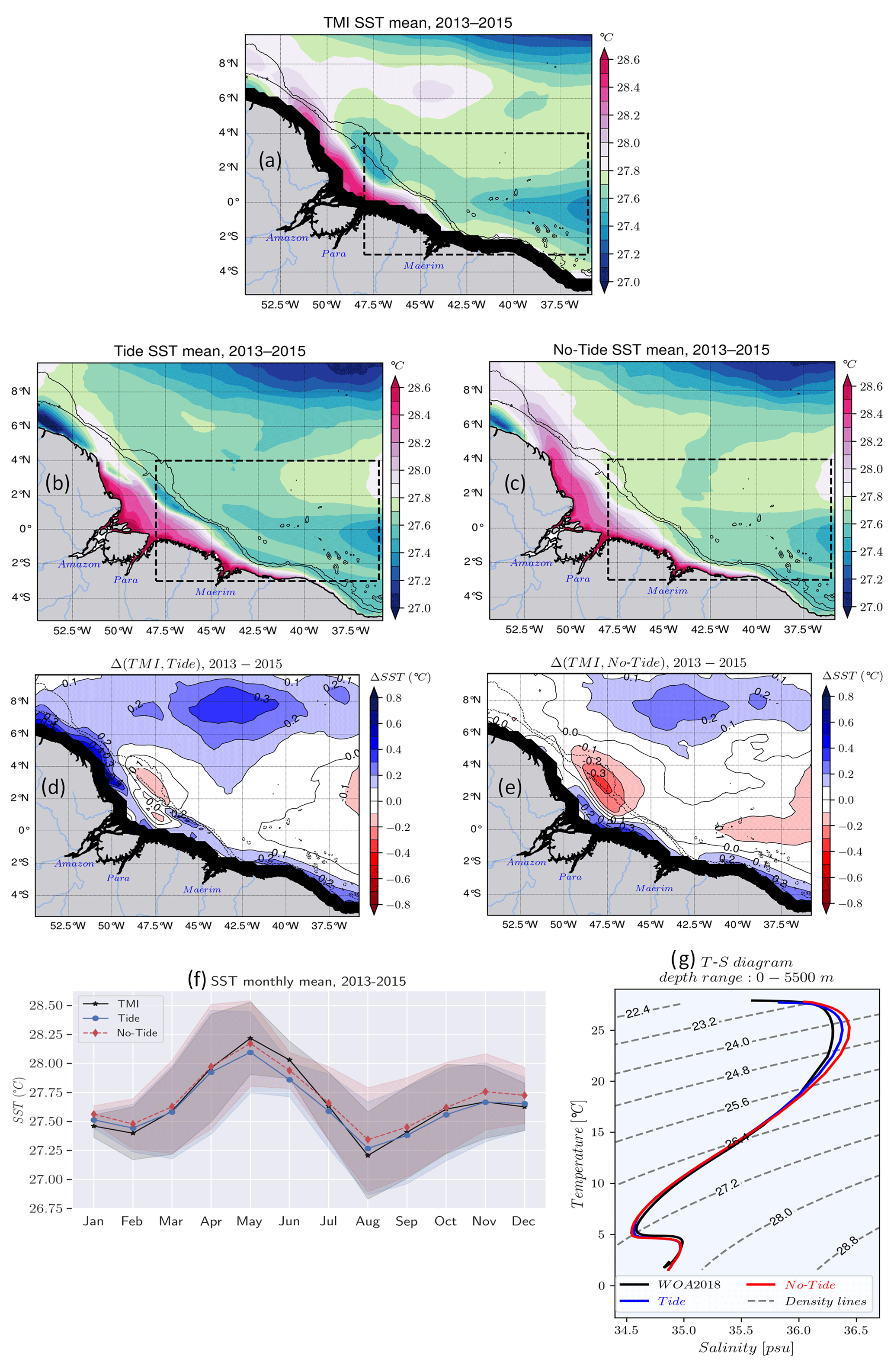
Figure 3 Validation of the model temperature for the whole period 2013–2015. Mean SST for (a) TMI with its black coastal mask, (b) the tidal simulation, (c) the non-tidal simulation, the difference (bias) in SST between TMI and (d) the tidal simulations and (e) the non-tidal simulation, and (f) the seasonal cycle of the SST of the three products averaged within the dashed box in upper panels covering IT pathways with values masked below the 200 m isobath; bands indicate variability according to standard deviation. Solid black lines in (a)–(c) and dashed black lines in (d)–(e) represent the 200 and 2000 m isobaths from the model bathymetry, while solid black lines in (d)–(e) represent bias contours. (g) Temperature–salinity (T-S) diagram of the mean properties in the same area as (f) from observed WOA2018 climatology (black line) and the tidal simulations (blue line) and non-tidal simulations (red line) for the water column from surface to 5500 m depth; dashed gray lines represent density (σ_θ) contours.

To gain insight into our model performance along the depth, we used the mean WOA2018 climatology (2005–2017) and simulation data (salinity and temperature) for the 3 years 2013–2015, averaged in the same region as in Fig. 3f. Figure 3g shows the temperature–salinity (T-S) diagram for WOA2018 and the two simulations. The data are averaged in the box as before, and we use σ_θ [ρ−1000] to represent the density contours, with ρ the water density. Both simulations exhibit similar patterns as WOA2018 for deeper waters, i.e., T<17 ^∘C and σ_θ>25.6 kg m⁻³. However, there are minor discrepancies for the surface layer waters, i.e., T>17 ^∘C and $\mathrm{22.4}>{\mathit{\sigma }}_{\mathit{\theta }}<\mathrm{25.6}$ kg m⁻³. At that level, the tidal simulations better reproduce the T-S profile of the observations. These slight differences between WOA2018 observations and the two simulations, especially with the tidal simulations, further demonstrate the ability of our model to reproduce the observed water mass properties.

4 Results

In this section, we present the influence of tides on temperature, the associated processes, and the impact on the atmosphere–ocean net heat exchange. The analyses were performed on a seasonal scale between April–May–June (AMJ) and August–September–October (ASO) for the 3 years 2013–2015.

4.1 Tide-enhanced surface cooling

During the first season, warm waters, which are defined as >27.6 ^∘C, dominate near the coast, especially in the middle shelf and in the southeast, and cold waters are present offshore north of 6^∘ N (Fig. 4a–c). Off the mouth of the Amazon River, water colder than 28.2 ^∘C spreads between 43–51^∘ W for TMI SST (Fig. 4a) and tidal simulations (Fig. 4b), while warmer waters are present in the same area for the simulations without tides (Fig. 4c). Figure 4d–f show the SST, averaged over the ASO season. TMI SST (Fig. 4d) shows an upwelling cell represented by the extension of the 27.2 ^∘C isotherm (white dashed contour) along the slope to about 49^∘ W–3^∘ N towards the northeast of the region, which forms the extension of the ACT. This extension also exists in the tidal simulations (Fig. 4e), whereas ≤27.2 ^∘C waters are not crossing 45.5^∘ W and remain in the Southern Hemisphere in the simulations without tides (Fig. 4f). This means that waters colder than 27.2 ^∘C can only extend further into the northeast because of tides. In addition, we can note that the mean SST shows a very contrasting distribution between the two seasons. There are warm waters along the shelf and cold waters offshore during the AMJ season (Fig. 4a–c). This is followed by warming along the Amazon plume and offshore, and an upwelling cell in the southeast (Fig. 4d–f).

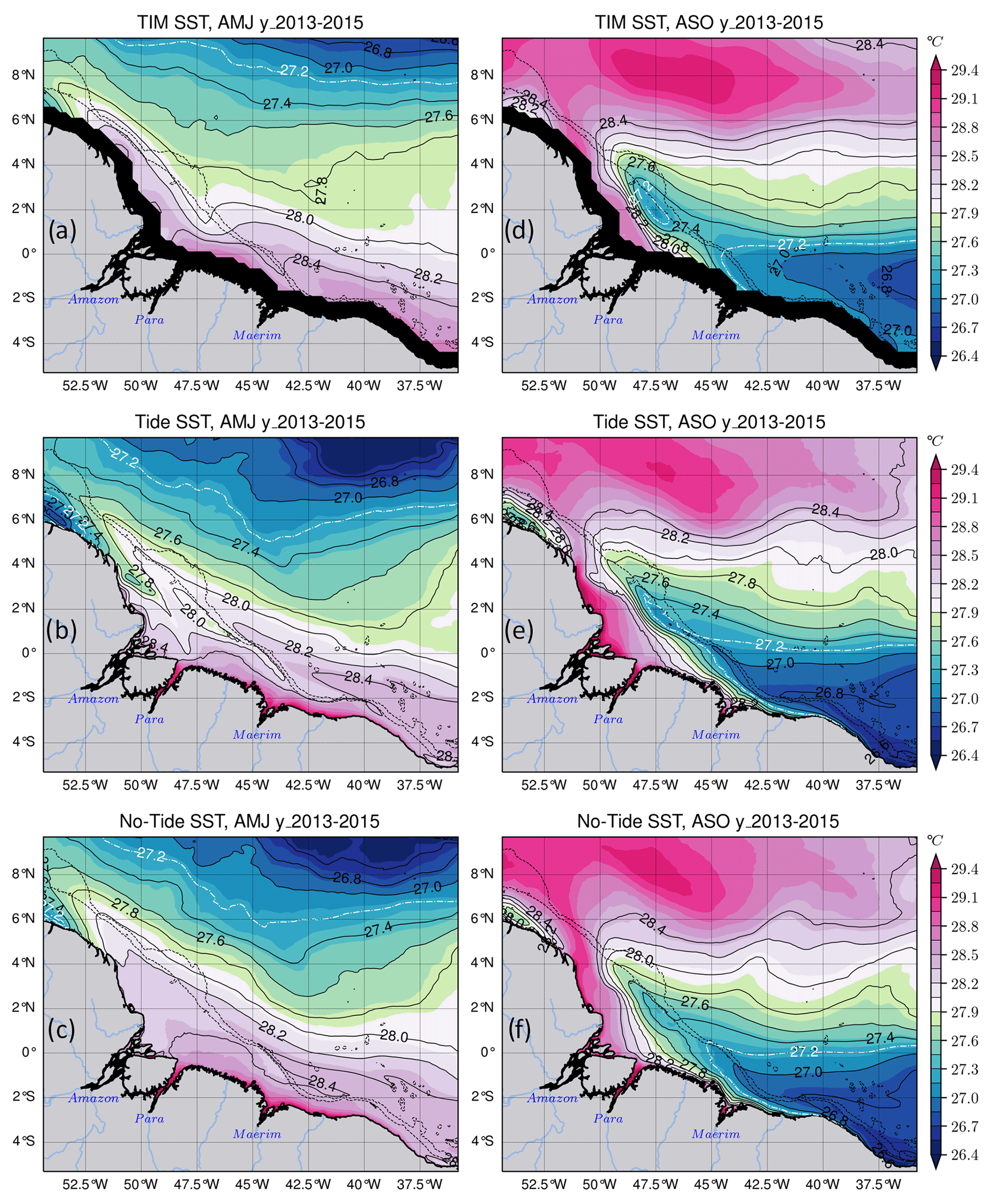
Figure 4 The 2013–2015 seasonal SST mean. Panels (a)–(c) stand for the AMJ season for TMI with its black coastal mask, the tidal simulations, and the non-tidal simulations, respectively; the same information is shown in (d)–(f) but for ASO season. The dashed white and solid black lines represent the temperature contours. Dashed black lines in all panels stand for the 200 and 2000 m isobaths from the model bathymetry.

The general impact of the tides, illustrated by the SST anomaly between the tidal and the non-tidal simulations, is a cooling over a large part of the study area with maxima up to 0.3 ^∘C (Fig. 5a–b). For ASO, tides induce a warming (>0.3 ^∘C) on the shelf at the mouth of the Amazon River (Fig. 5b), while for AMJ it is a cooling of the same intensity (Fig. 5a). That difference will be further discussed. Out of the shelf, the structure of temperature anomaly varies depending on the season, probably because of seasonal mesoscale variability.

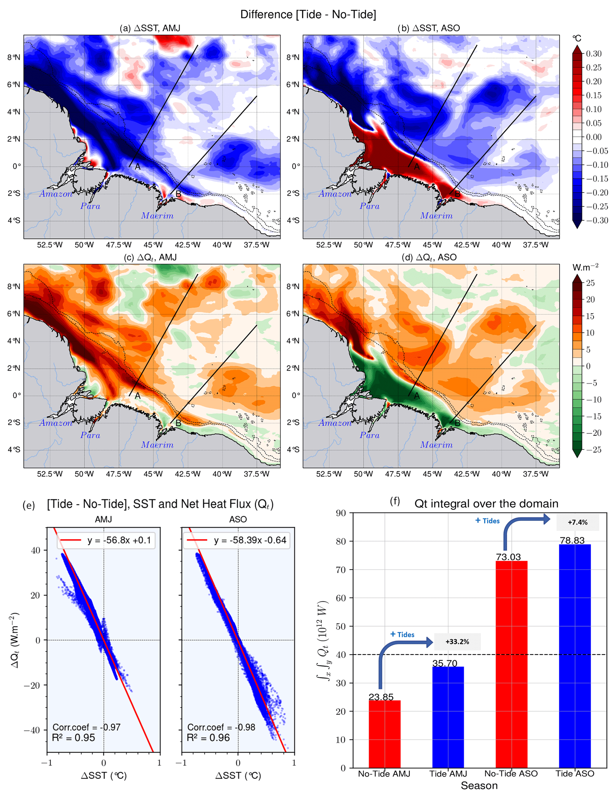
Figure 5 Relationship between the SST and the atmosphere–ocean net heat flux (Q_t): SST anomaly (tide–no tide) in AMJ (a) and ASO (b) seasons, Q_t anomaly in AMJ (c) and ASO (d) seasons, (e) correlation between Q_t anomaly and SST anomaly for each season, and (f) domain-integrated Q_t for both seasons of each simulation. Dashed black lines in (a)–(d) stand for the 200 and 2000 m isobaths from the model bathymetry.

4.2 Impact of the tides on the atmosphere-ocean net heat flux

The atmosphere–ocean net heat flux (Q_t) reflects the balance of incoming and outgoing heat fluxes across the atmosphere–ocean interface (see Moisan and Niiler, 1998; Jayakrishnan and Babu, 2013). During AMJ, tides mainly induce positive Q_t anomalies over the whole domain. The average values are around 25 W m⁻² in the plume and the Amazon retroflection to the northeast and along A and B (Fig. 5c). Negative SST anomalies (∼0.3 ^∘C) occur throughout the domain in the same location. During the ASO season, at the mouth of the Amazon, there are negative Q_t anomalies but of the same magnitude as during the previous season (Fig. 5d). At this location, positive temperature anomalies (∼0.3 ^∘C) are observed (Fig. 5b). Elsewhere, there are positive Q_t anomalies and negative SST anomalies. It therefore appears that negative SST anomalies induce positive Q_t anomalies and vice versa. Hence, the spatial structures of Q_t anomalies and SST anomalies fit together for the two seasons. There is a strong negative correlation of 0.97 with a significance of R²=0.95 for the AMJ season and almost the same in ASO season, with 0.98 and 0.96, respectively, for the correlation and its significance (Fig. 5e). This is consistent with the fact that the atmosphere and the underlying ocean are balanced. Following this, the SST cooling induced by upwelled cold water will try to upset this balance. As a result of this, an equivalent variation in the net heat flux from the atmosphere to the ocean will attempt to restore it.

In Fig. 5f the integral over the entire domain of the net heat flux for each season and for each simulation is shown. During the AMJ season, Q_t increases from 23.85 TW (1 TW = 10¹² W) for the non-tidal simulations to 35.7 TW for the tidal simulations, i.e., an increase of 33.2 %. That is, the tides are responsible for a third of Q_t variation. This is very large compared to what is observed elsewhere in other IT hotspots (e.g., 15 % in the Solomon Sea, Tchilibou et al., 2020). During the second season, there is a smaller increase in Q_t of about 7.4 % between the two simulations, i.e., from 73.03 to 78.83 TW for the non-tidal and tidal simulations, respectively (Fig. 5f).

It is also worth noting the significant difference in integrated Q_t between the two seasons. The values are less than 36 TW during the AMJ season, whereas they are around twice as high, >73 TW, during the ASO season. Given that colder SSTs induce a stronger Q_t, these higher values are likely related to the arrival of cold waters from ACT, which forms upwelling cells (Fig. 4d–f) with a secondary tidal effect.

4.3 Vertical structure of temperature along internal tide pathways

To further analyze the temperature changes between the two simulations, we made vertical sections following the path of IT radiating from sites A and B (respectively black and red line in Fig. 2f). Here, only the transects following the pathway A are presented, since the vertical structure is similar following pathway B especially for AMJ season and because some processes tend to be null along pathway B during the ASO season. The mixed layer refers to a quasi-homogenous surface layer of temperature-dependent density that interacts with the atmosphere (Kara et al., 2003). Its maximum depth, also known as mixed-layer depth (MLD), is defined as the depth where the density increases from the surface value, due to temperature change of $\left|\mathrm{\Delta }T\right|=\mathrm{0.2}$ ^∘C with constant salinity (e.g., Dong et al., 2008; Varona et al., 2019).

Figure 6 shows the vertical sections of temperature for the two seasons following A. In AMJ season, over the slope and near the coast, cold waters (<27.6 ^∘C) remain below the surface at ∼20 m for the tidal simulations (Fig. 6a) and deeper at ∼60 m for the non-tidal simulations (not shown). The cold waters rise to the surface more than 400 km offshore for both simulations. In surface layers (<40 m), the temperature anomaly is more than −0.8 ^∘C at the shelf beak and less than −0.2 ^∘C elsewhere (Fig. 6b). Further down (<60 m) the water column, this anomaly becomes much larger along the transect. Above that thermocline (<120 m), the simulations with tides are colder by 1.2 ^∘C from the slope, where IT are generated and following their propagation pathway. Conversely, below the thermocline, the tidal simulations are warmer by the same intensity along the propagation path and down to ∼300 m depth (Fig. 6b). In the AMJ season, the thermocline depth is about 100±15 m and MLD is about 40±20 m (Fig. 6a). They both have a very weak slope between the coast and the open ocean. Over the whole domain, the thermocline is deeper by about 15 m on average in the non-tidal simulations, following the propagation paths of internal tides, on the Amazon shelf and plume (Fig. 6c). Similarly, the MLD in the non-tidal simulations is deeper by approximately 10 m over the shelf, ∼4 m along IT propagation paths, and close to zero in the Amazon plume (Fig. 6d).

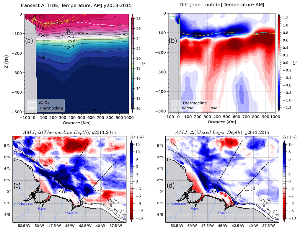
Figure 6 Water mass properties for the AMJ season: (a) vertical section of the temperature of the tidal simulations following transect A, the dashed yellow and the solid black lines are the temperature and density (σ_θ) contours, respectively. The dashed black and white ticker lines are the thermocline and MLD, respectively. (b) The temperature anomaly for the same vertical section, dashed yellow and cyan lines are the thermocline depth for the tidal and non-tidal simulations, respectively. (c) Thermocline depth anomaly and (d) MLD anomaly for the whole domain. The blue (vs. red) color shading in the MLD or the thermocline depth anomaly means that tides raise (vs. deepen) them. Solid black lines in lower panels stand for the 200 and 2000 m isobaths from the model bathymetry.

In the ASO season, cold waters previously confined below the surface during the previous season (AMJ) rise to the surface. These cold waters extend over the slope and up to about 150 km offshore in the non-tidal simulations (not shown) and up to 250 km offshore in the tidal simulations (Fig. 7a). The 27.2 ^∘C isotherm only reaches the surface above the slope in the tidal simulations and remains below the surface (∼30 m) in the non-tidal simulations (not shown). This aligns with the absence of that isotherm at this location in the corresponding SST map (Fig. 4f). For the tidal simulations, the temperature anomaly in the ASO season is smaller ($\sim -\mathrm{0.4}$ ^∘C, Fig. 7b) in the surface layers (<40 m) near the coast compared to the AMJ season (Fig. 6b). In contrast, during the ASO season, this cooling can drive more SST anomalies along A (−0.3 ^∘C, Fig. 5b). A stronger cooling of about 1.2 ^∘C occurs deeper between 60 and 140 m depth, and a warming of about 1.2 ^∘C below, which extends less offshore than during the AMJ season, 650 km vs. ∼1000 km. In the ASO season, the coastward slope of the thermocline and MLD becomes steeper compared to the AMJ season. In both simulations, there is a dip of ∼80 m, i.e., ∼60 m offshore and ∼140 m inshore, for the thermocline (Fig. 7a), and a dip of ∼40 m, i.e., ∼30 m offshore and ∼70 m inshore, for MLD (Fig. 7a). Over the entire domain, tides reduce the thermocline depth by ∼6 m on the shelf and ∼12 m at the plume and far offshore along the propagation path of A (Fig. 7c) and the MLD by about 10 m along the shelf and ∼4 m along the propagation path of A (Fig. 7d).

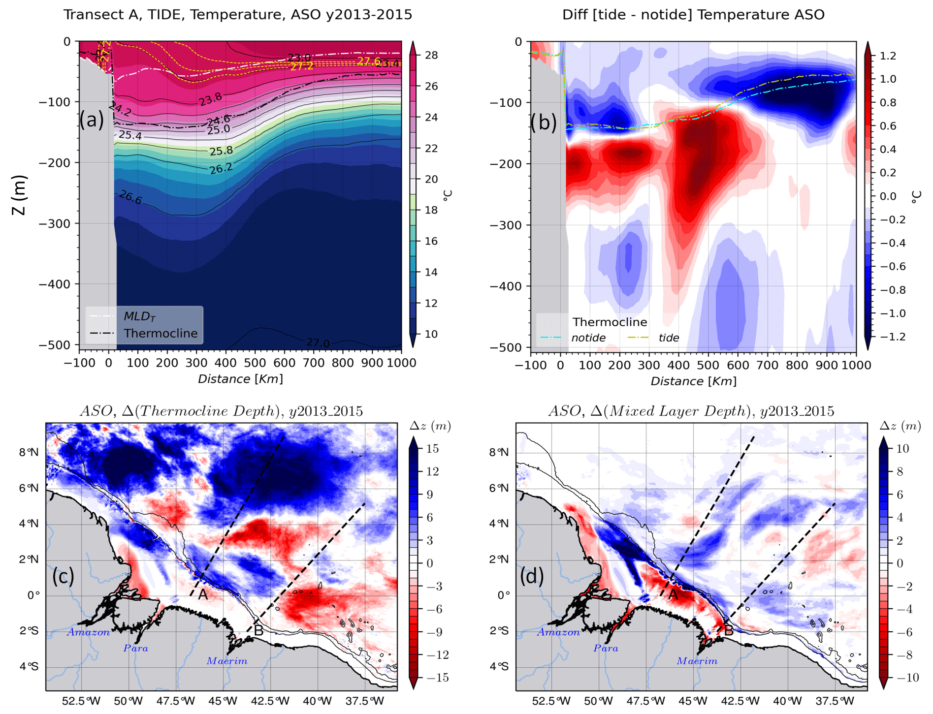
Figure 7 The same as Fig. 6 but for the ASO season.

Between the two seasons, there is also a change in the vertical density gradient between the coast and the open sea. In tidal simulations, during the AMJ season the isopycnals layers are thin near the coast and thicken towards the open sea (Fig. 6a). This means that a strong stratification is present near the coast and decreases towards the open sea. In contrast, during the ASO season the isopycnal layers are thicker near the coast and tight offshore (Fig. 7a). As the result of this, the stratification is weaker inshore than offshore. This clearly highlights a seasonality in the vertical density gradient profile in agreement with Tchilibou et al. (2022). Note that this behavior also appears in the simulations without tides (not shown). The transects of the temperature anomaly show that tides influence the temperature in the ocean from the surface to the deep layers, with a greater effect on the first 300 m. One avenue we explore in this paper is creating a better understanding of what processes are at work that explain these temperature changes.

4.4 What are the processes involved?

To explain the observed surface and water column temperature changes, we computed and analyzed the terms of the heat balance equation (see Sect. 2.3.2, Eq. 6) for both seasons (AMJ and ASO).

4.4.1 Vertical diffusion of temperature

Figure 8 shows the vertical temperature diffusion tendency (ZDF). ZDF is averaged between 2–20 m, i.e., within the mixed layer. For the AMJ season, ZDF in the tidal simulations (Fig. 8a) shows a negative trend (i.e., cooling) in the whole domain. The maximum values ($>\left|\mathrm{0.4}\right|$ ^∘C d⁻¹) are located along the slope where IT are generated and on their propagation path. There is a larger horizontal extent along A of ∼700 km from the coasts compared to B, where it is ∼300 km from the coasts. Elsewhere, ZDF is weak ($>-\mathrm{0.1}$ ^∘ C d⁻¹). For the non-tidal simulations (Fig. 8b), ZDF is weak over the entire domain ($>-\mathrm{0.1}$ ^∘C d⁻¹). In ASO season, the tidal simulations (Fig. 8c) show a decrease in the ZDF near the coast (<100 km) and a strengthening offshore along A compared to the previous season but with the same cooling trend ($<-\mathrm{0.4}$ ^∘C d⁻¹). Along B, it tends to be null both at the coast and offshore (Fig. 8c). In addition, the mesoscale circulation and eddy activity intensify during this season. To the northeast, between 4–8^∘ N and 47–53^∘ W, there is a cooling on the shelf of ∼0.3 ^∘C d⁻¹ with eddy-like patterns in the tidal simulations (Fig. 8c). The processes by which these features might arise are discussed in more detail in Sect. 5. Unsurprisingly, ZDF is weak everywhere for the non-tidal simulations (Fig. 8d). ITs are the dominant driver of vertical diffusion of temperature along the shelf break and offshore, while the mixing induced by barotropic tides prevail on the shelf.

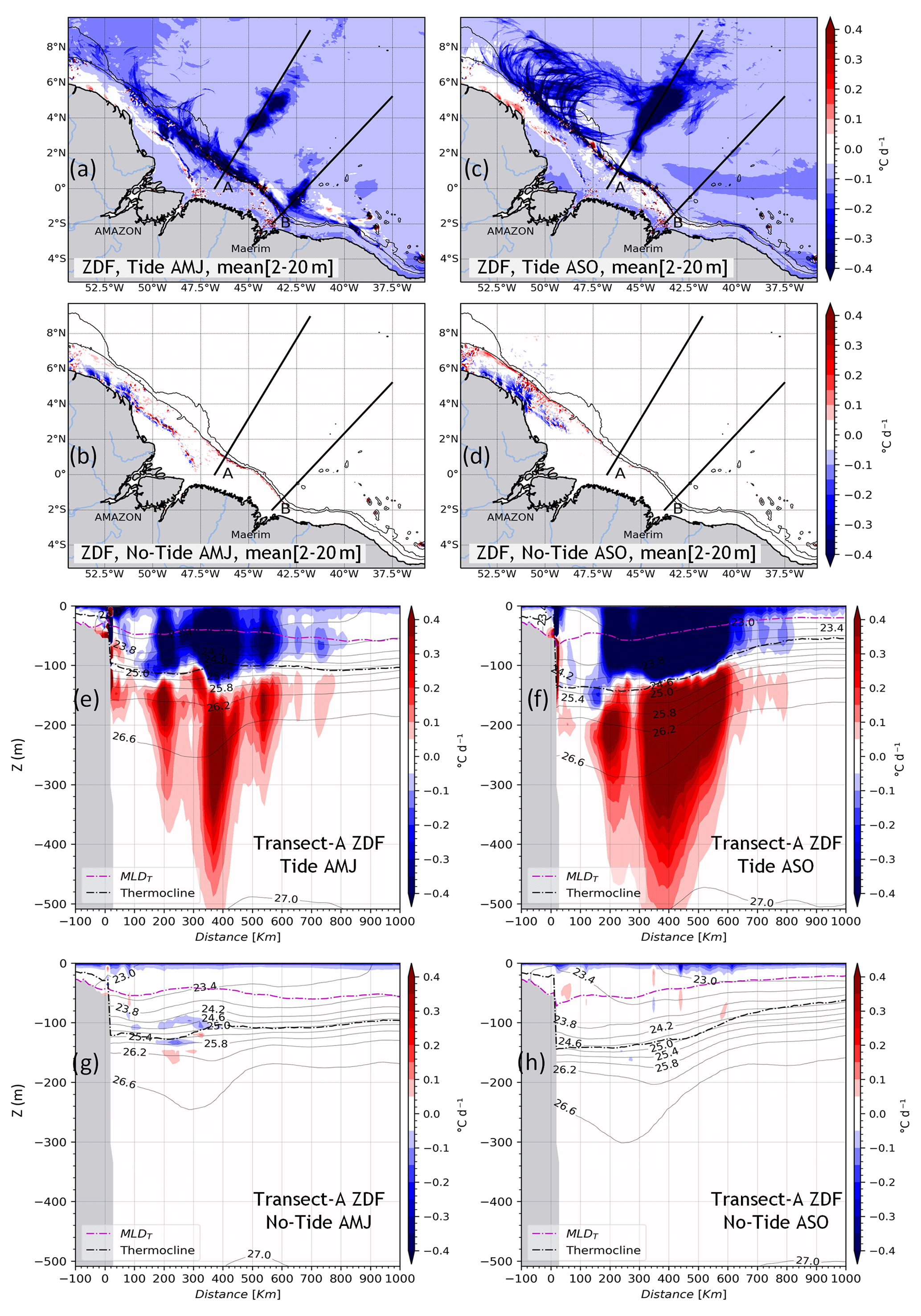
Figure 8 The vertical diffusion tendency of temperature (ZDF) for both seasons. The vertical mean between 2–20 m for the AMJ season in tidal (a) and non-tidal (b) simulations and for the ASO season in tidal (c) and non-tidal (d) simulations. Vertical sections of ZDF following transect A in the tidal simulations for (e) AMJ and (f) ASO seasons and for the non-tidal simulations for the (g) AMJ and (h) ASO seasons. Solid black lines in (a)–(d) stand for the 200 and 2000 m isobaths from the model bathymetry, while they represent the density (σ_θ) contours in (e)–(h). The magenta and dashed black lines in (e)–(h) represent MLD and the thermocline depth, respectively.

On the vertical following A, there are opposite-sign ZDF values with a mean magnitude of $\sim \left|\mathrm{0.4}\right|$ ^∘C d⁻¹. These values are centered around the thermocline for the simulations with tides in the two seasons AMJ and ASO (Fig. 8e and f, respectively). There is a cooling trend above the thermocline and a warming trend below. The average vertical extent is up to ∼350 m depth for the maximum values but exceeds 500 m depth for the low values (<0.1 ^∘C d⁻¹). As for the horizontal averages (Fig. 8a and c), from one season to another there is a weakening of ZDF above the slope and a strengthening offshore (Fig. 8e and f, for AMJ and ASO, respectively). Furthermore, offshore ZDF maxima are discontinuous and spaced about 140–160 km apart during the AMJ season (Fig. 8e) but are more continuous for the ASO season (Fig. 8f). For the non-tidal simulations, the mean ZDF tends to be null in the ocean interior but remains quite large ($>-\mathrm{0.2}$ ^∘C d⁻¹) in the thin surface layer during the two seasons (Fig. 8g–h).

Furthermore, it is worth noting that the maxima of the ZDF follow the maxima of the baroclinic tidal energy dissipation along IT propagation's pathway (Fig. 2f). This proves that the dissipation of IT causes vertical mixing that enhances SST cooling. In addition, this temperature diffusion contributes to greater subsurface cooling within the mixed layer and warming in the deeper layers beneath the thermocline.

The seasonality of the stratification highlighted above could explain why the ZDF is stronger along the slope and the near-coastal pathway B during the AMJ season (Fig. 8a and e), and why in the ASO season ZDF is weaker along the slope, close to zero following B, and reinforced offshore of A (Fig. 8c and f). Previous studies have shown that stratification influences the generation of internal tides and controls their modal distribution. Here we show that stratification also plays a role in the fate of these internal tides, in this case on their dissipation. The stratification could determine where ITs dissipate their energy in the water column, as mentioned by de Lavergne et al. (2020).

4.4.2 Advection of temperature

The vertical (z–ADV) and the horizontal (h–ADV) terms of the temperature advection tendency are averaged in the same depth range as above for the two seasons.

Vertical advection of temperature

Tides fail to generate vertical temperature advection within surface layers. As expected, z–ADV is almost null throughout the region in that depth-range (Fig. 9a–d). Nevertheless, for both seasons, there are extreme values located in the northwest on the plateau between 54–50^∘ W and 3–6^∘ N with the same intensity in the two simulations (<0.3 ^∘C d⁻¹). But deeper, vertical sections (Fig.9a–h) show an intensification of z–ADV of about ±0.8 ^∘C d⁻¹ located below the MLD and seems to be centered around the thermocline, with a vertical extension from 20–200 m depth. In addition, z–ADV is stronger in tidal simulations during both seasons (Fig. 9e–f) and presents sparse extrema offshore (>300 km) for the non-tidal simulations (Fig. 9g–h). For the simulations with tides, z–ADV appears to be dominated by a cooling trend, with a marked hotspot on the slope followed by other hotspots offshore. These extreme values are spaced about 120–150 km apart, i.e., a mode-1 wavelength as for the baroclinic tidal energy dissipation (Fig. 2f). Note that for both simulations (Fig. 9e–h), the extreme values are located within the narrow density (σ_θ) contours (23.8–26.2 kg m⁻³), i.e., within the pycnocline. The location of the extreme values of z–ADV at the shelf break and along IT propagation pathways and its negative sign suggest that the diffusive part of the advection scheme may account significantly in z–ADV.

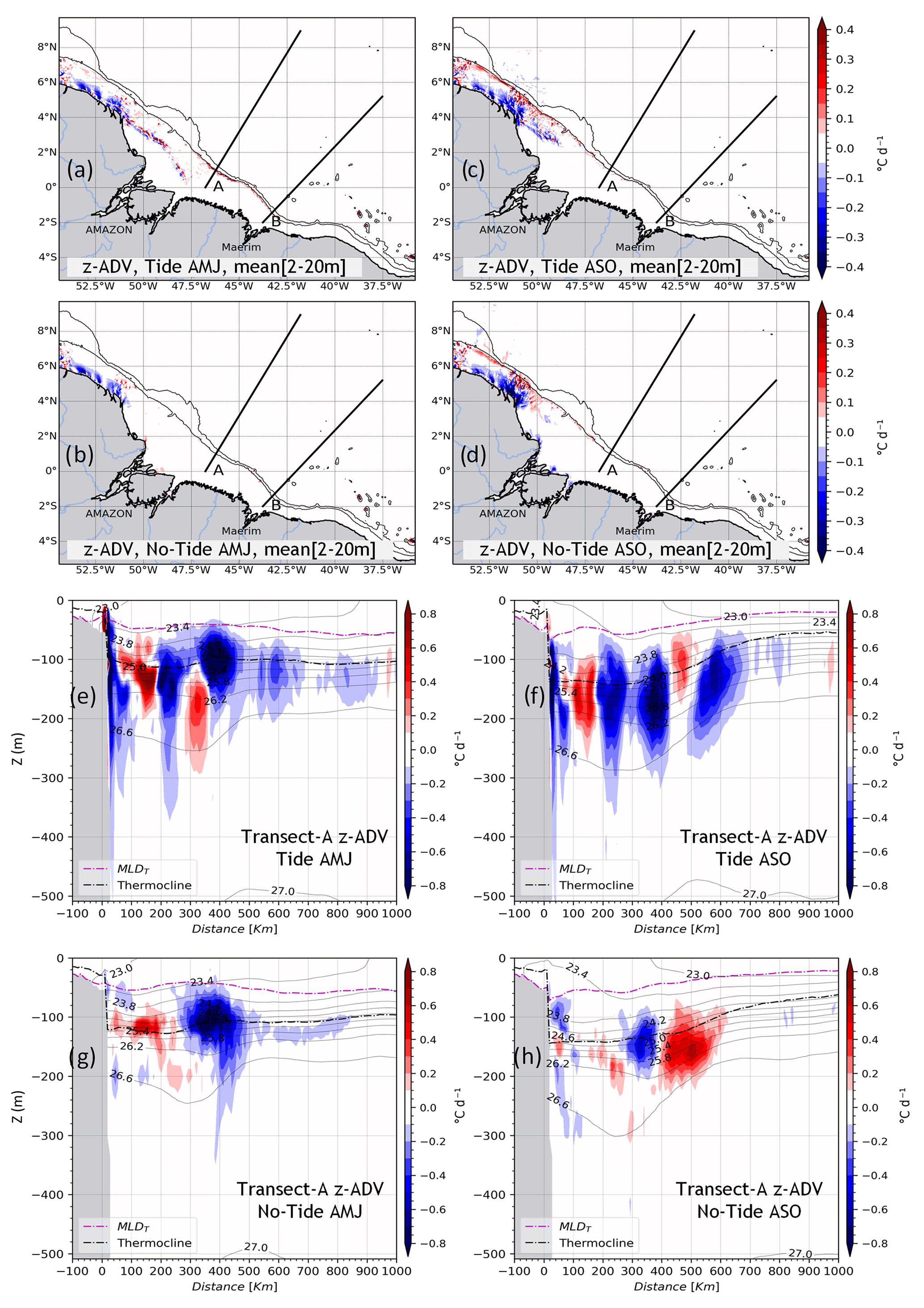
Figure 9 The same as Fig. 8 but for the vertical advection of temperature (z–ADV).

Horizontal advection of temperature

Horizontal advection of temperature (h–ADV) is defined as the sum of the zonal (x–ADV) and meridional (y–ADV) terms of temperature advection tendency. As for z–ADV, the mean of h–ADV tends to be null over the entire domain in the surface layers for both seasons in both simulations (Fig. 10a–d). Nevertheless, weak extrema exist in the northwest of the plateau between 3–7^∘ N and 54–50^∘ W. These intensify during the ASO season in both simulations, $\sim \pm \mathrm{0.2}$ ^∘C d⁻¹; see Fig. 10c and d for the tidal and non-tidal simulations, respectively. In AMJ season, h–ADV is slightly stronger, ∼0.1 ^∘C d⁻¹, around sites A and B in the tidal simulations (Fig. 10a), which appears to be related to IT generated along the slope. However, there is a slight distinction between the two simulations in the surface layers, suggesting that tides have a minimal effect on h–ADV, as expected. Consequently, h–ADV has a negligible influence on the cold-water tongue observed in the surface SST during the ASO season (Fig. 4d–f).

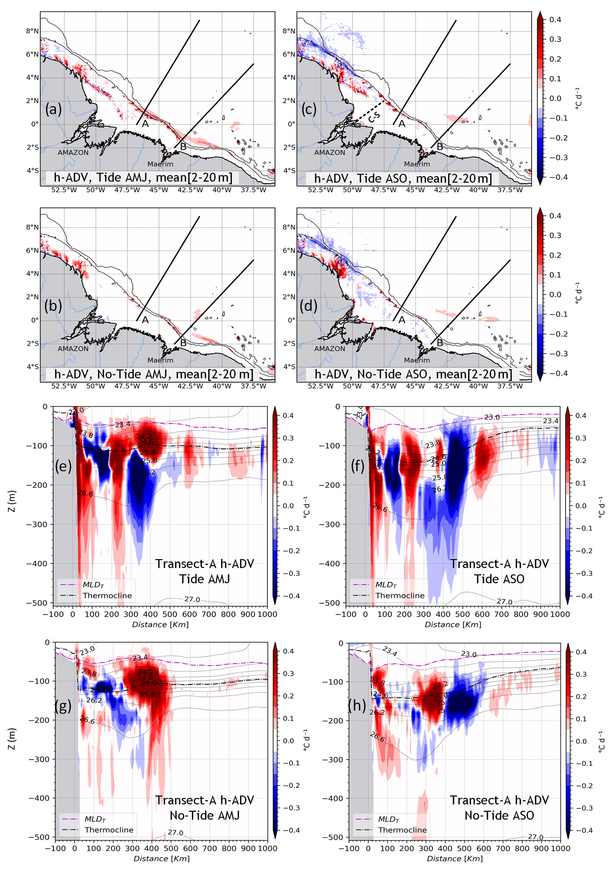
Figure 10 The same as Fig. 8 but for the horizontal advection of temperature (h–ADV = x–ADV + y–ADV). The dashed line from the Amazon River mouth toward the outer shelf in (b) indicates the cross-shore transect (C-S) used further on.

Along the vertical following A, h–ADV maxima are confined below the mixed-layer depth. The tidal simulations (Fig. 10e–f) exhibit significantly more intense values compared to the non-tidal simulations (Fig. 10g–h). The h–ADV contributes to both warming and cooling of the temperature, with a magnitude of about ±0.4 ^∘C d⁻¹, extending from the slope to over 500 km offshore. In both seasons, the average vertical extension lies between the surface and 400 m depth for the tidal simulations, and between 20–300 m depth for the non-tidal simulations. Similarly to z–ADV, h–ADV is stronger within the pycnocline. In the tidal simulations, a warming effect is observed above the slope (0.4 ^∘C d⁻¹), reaching the surface in both seasons. This vertical excursion is also observed for ZDF and z–ADV, and it is a marker of local dissipation of IT at their generation sites. It is noteworthy that the location of h–ADV maxima does not coincide with the dissipation hotspots of IT, in contrast of ZDF and z–ADV.

4.4.3 Heat budget balance

From the sections above, it is evident that IT-induced mixing within the mixed layer emerges as the primary driver among the ocean's internal processes in explaining changes in SST. However, below MLD, advective processes play a more significant role in structuring temperature. Figure 10 presents the average of the terms of the Eq. (6) below MLD within the depth range of 60–400 m. The analysis focuses on a specific region with latitude and longitude ranging between 0–6^∘ N and 40–48^∘ W, respectively. This region includes the two main IT paths, as well as a portion of the along-coast upwelling region. During the AMJ season, ADV is the dominant process over diffusion terms in both tidal (Fig. 11a) and non-tidal (Fig. 11b) simulations. However, in the ASO season, ADV only dominate in tidal simulations (Fig. 11c), while ZDF dominates in non-tidal simulations (Fig. 11d).

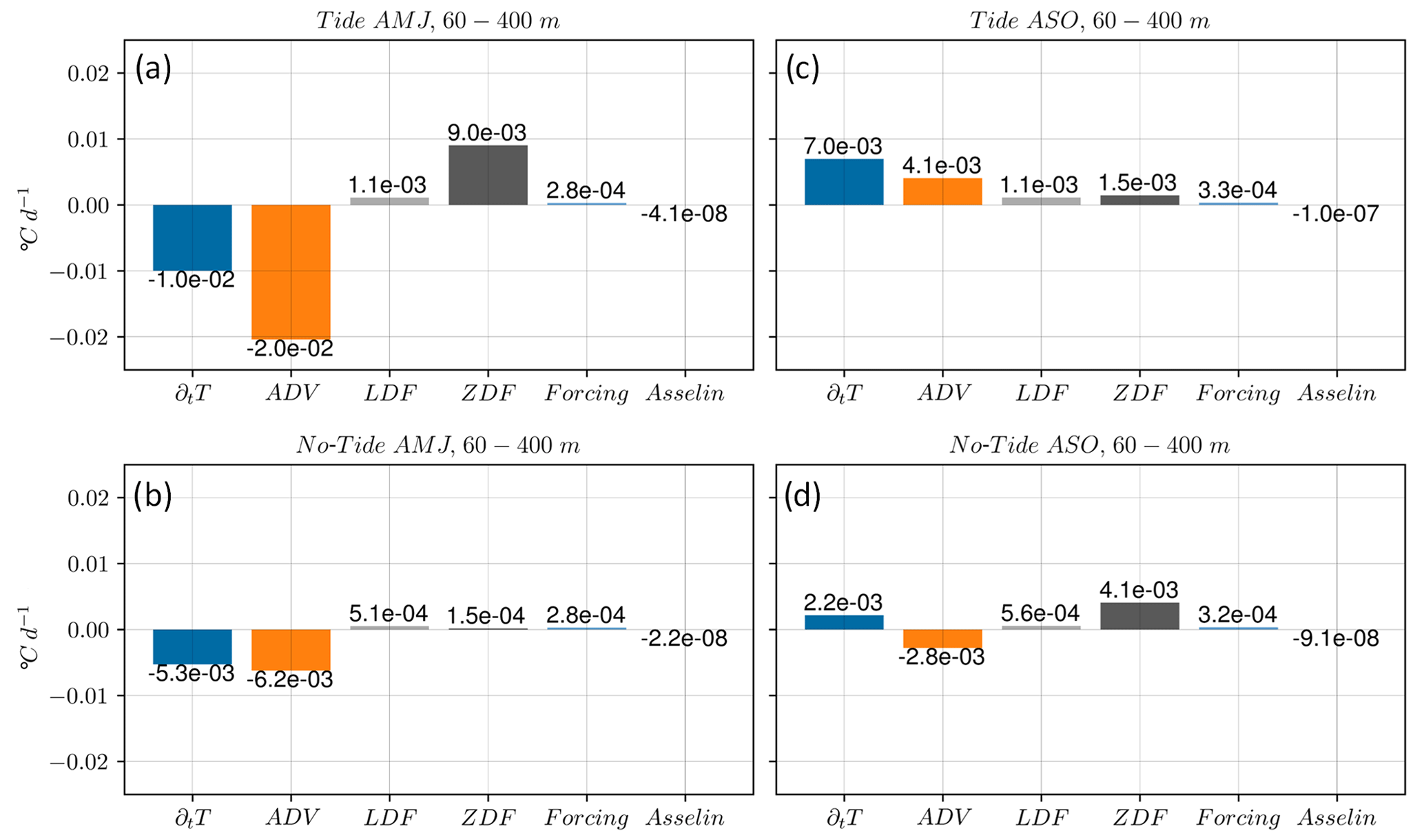
Figure 11 Three-dimensional heat budget equation terms averaged in region around IT trajectories between 0–6^∘ N and 48–40^∘ W and below the MLD between 60–400 m depth. Panels (a) and (c) are for the tidal simulations, (b) and (d) are for the non-tidal simulations, and (a)–(b) and (c)–(d) are for the AMJ and ASO seasons, respectively.

It therefore appears that ADV only has a considerable influence on temperature below MLD, contrasting with the study of Neto and da Silva (2014), which identifies ADV as the primary driver causing along-coast SST cooling. However, we can assume that advection and mixing are interconnected. In other words, the water masses that are advected below MLD may undergo mixing within the surface layers due to the overall mixing occurring throughout the water column. Additionally, it is worth mentioning that in our simulations Asselin has a negligible impact on temperature. Conversely, the forcing term does impact the temperature within the surface layers. However, we have not discussed this aspect in our analysis as our primary focus was on understanding the internal processes of the ocean.

5 Discussion

5.1 The mode-1 wavelength in the vertical terms of the heat budget equation

Along the vertical and towards the open ocean, both ZDF and z–ADV exhibit a wave-like structure, with patches that are spaced apart by about 120–160 km typical of mode-1 wavelength. However, during the ASO season, this pattern is not observed for ZDF. Instead, ZDF values appear more continuous along the transect, likely due to additional mixing caused by the breaking of incoherent ITs that intensify during that season. Furthermore, de Macedo et al. (2023) recently provided a detailed description of internal solitary waves (ISWs) in the same region based on remote sensing data. These ISWs originate from instabilities and energy loss or dissipation of ITs radiating from the slope, primarily along pathways A and B (Magalhaes et al., 2016). The first study demonstrated that the inter-packet distance of ISWs corresponds to the mode-1 wavelength. Interestingly, the positions of IT dissipation hotspots, as well as z–ADV patches in both seasons and ZDF patches, especially during the AMJ season, in our model align with the observed occurrences of ISWs (refer to Fig. 2 in their study). This provides evidence that our model accurately reproduces the location of IT dissipation.

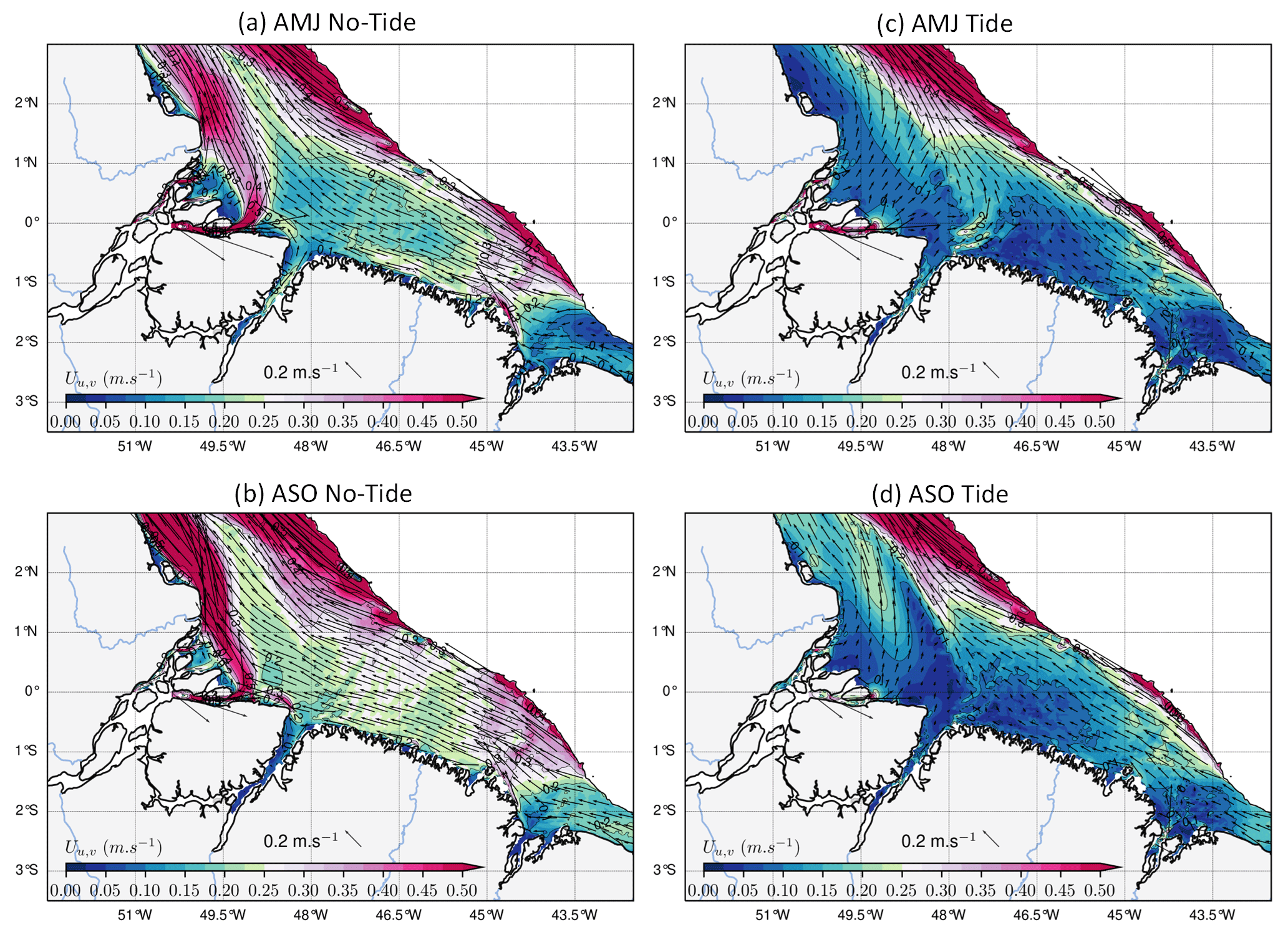
Figure 12 Seasonal mean of the mean current (U_u,v) at the shelf averaged between the surface and 50 m: the non-tidal simulations in are shown in (a) and (b), and the tidal simulations are shown in (c) and (d). Panels (a) and (c) stand for the AMJ season, while (b) and (d) stand for the ASO season. The color shading is the modulus of the current, and the black arrows represent its direction. Values beyond the 200 m isobath are masked.

5.2 Temperature changes over the shelf: two main competitive processes

In the simulation without tides, there is a strong along-coast current northwesterly exiting the mouth of the Amazon River (e.g., Ruault et al., 2020) with an average intensity lower than 0.5 m s⁻¹ in the first 50 m for both seasons (Fig. 12a–b). When including tides in the model, the latter study showed that there is an increase in the vertical mixing in the water column due to stratified-shear flow instability, which weakens and deflects the along-coast current northeastwards at the mouth of the Amazon River (Fig. 12c–d) and favors cross-shore export of water. We can therefore establish that there are at least two processes at work, (i) vertical mixing and (ii) horizontal transport, backed by ZDF and h–ADV, respectively. We then looked at the latter two processes along the vertical following the cross-shore transect (C-S) defined in Fig. 10c. Hereafter, “inner mouth” refers to the part of the transect within 200 km from the shore, whereas “outer shelf” refers to the part beyond.

During the AMJ season, the flow of the river becomes dominant in the inner mouth of the region. The tide-induced vertical mixing in the narrow water column results in the warming and deepening of the thermocline (Fig. 13a–b). Conversely, on the outer shelf, this mixing occurs in a thicker water column, leading to cooling above the thermocline and warming below (Fig. 13a). This pattern extends across the shelf and along the pathways of internal tides, as shown in Sect. 4.4.1 (refer to Fig. 8a and e). In this season, the weaker circulation may result in low values of h–ADV (Fig. 13b). Therefore, during the first season, the dominant process that explains the average negative SST anomaly over the shelf appears to be vertical mixing.

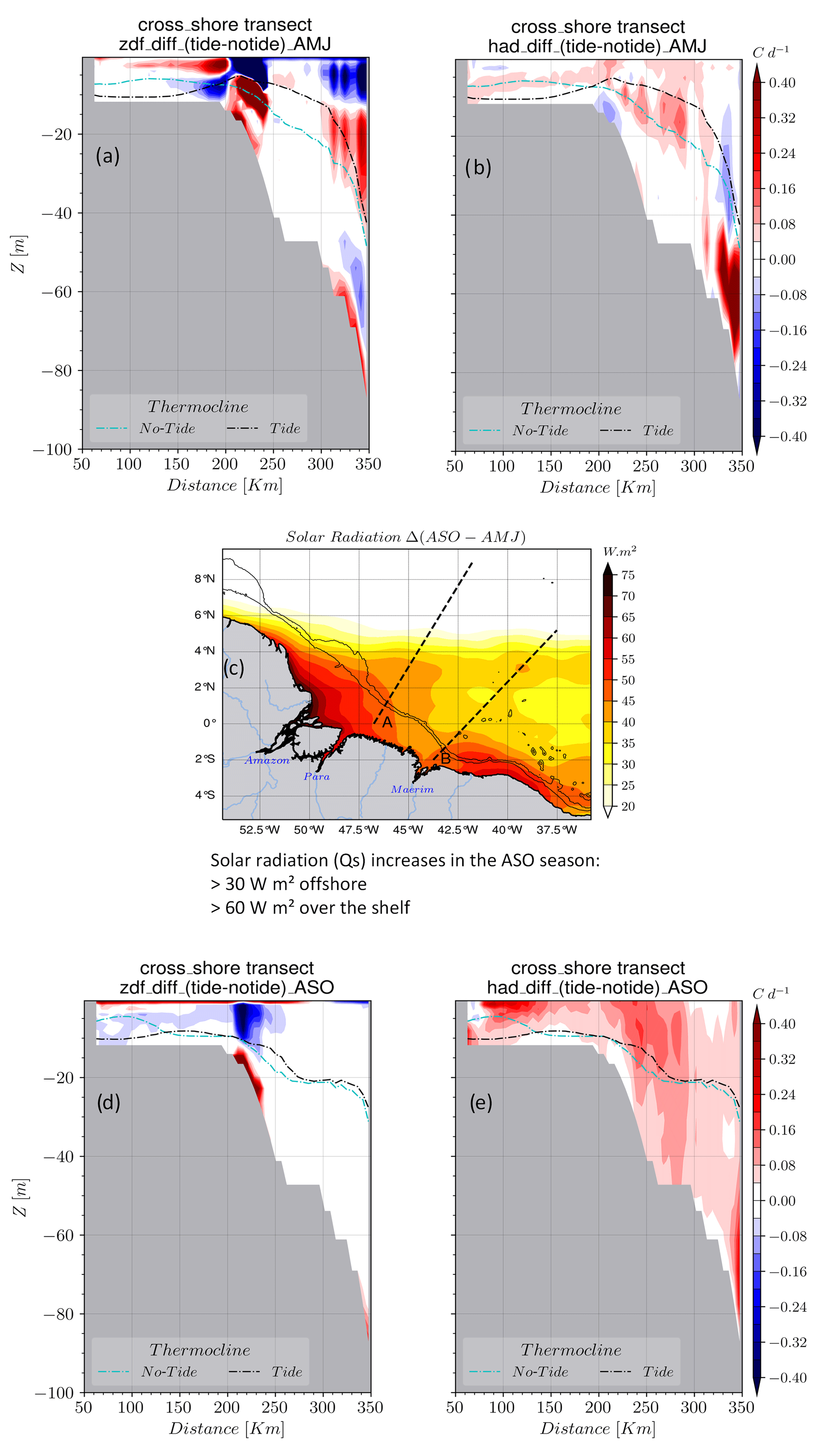
Figure 13 The cross-shore transect of the ZDF anomaly for the (a) AMJ and (b) ASO seasons and (c) the difference in solar radiation between ASO and AMJ seasons. Solar radiation increases during the ASO season, with greater intensity on the shelf. The cross-shore transect of the h–ADV anomaly for (d) AMJ and (e) ASO seasons.

During the second season, there is a significant increase in solar radiation on the shelf, with an average value of 60 W m⁻², compared to the previous season (Fig. 13c). Additionally, the average depth of the thermocline deepened further offshore (Fig. 13d and e). In this season, mixing processes lead to warming in the thin surface layer, specifically at depths of less than 2 m (Fig. 13d). NBC is stronger, resulting in an increase in the transport over the shelf (Prestes et al., 2018). It is also important to consider the small mean tidal residual transport (Bessières et al., 2008), which reinforces the stronger current transport. These factors contribute to a more dynamic region and an increase in h–ADV (Fig. 13e). Consequently, h–ADV plays a significant role in determining SST on the shelf. For this season, the combination of these two processes explains the observed positive SST anomaly.

Additionally, from the AMJ to ASO seasons, there is a notable deepening of the thermocline depth on the outer shelf. This observation has previously been highlighted by Silva et al. (2005) from REVIZEE (Recursos Vivos da Zona Econômica Exclusiva) campaign data, further validating our simulations.

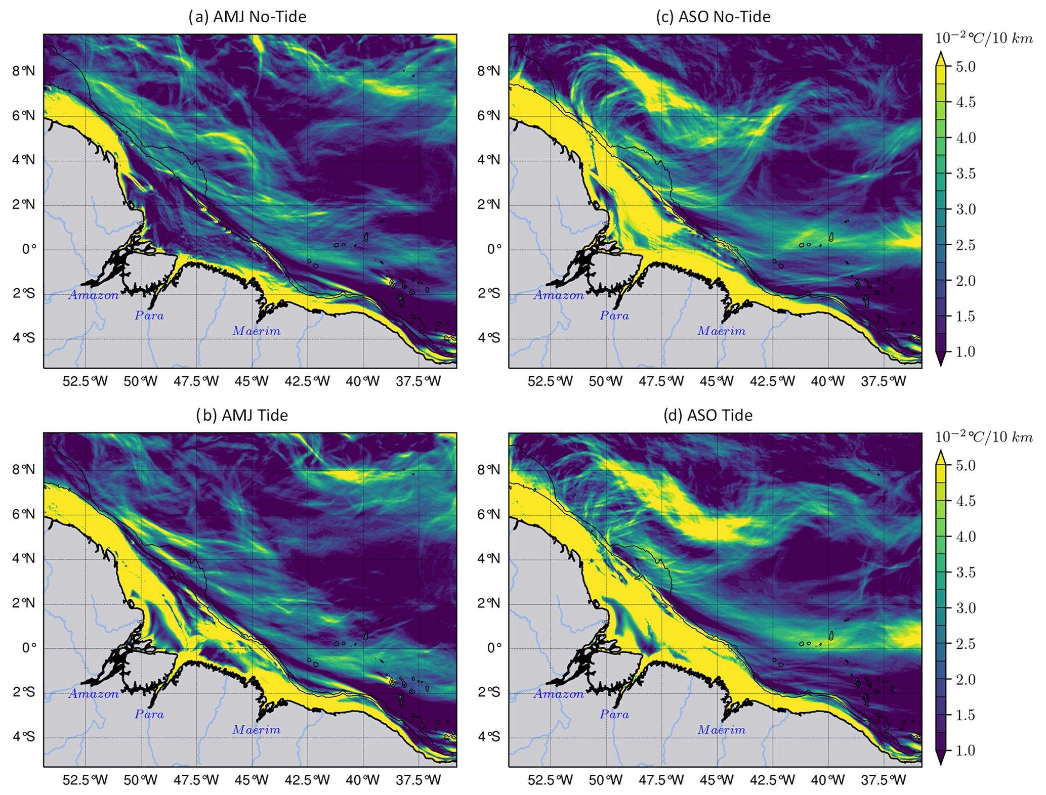
Figure 14 The horizontal gradient of the temperature (∇T) averaged between 2–20 m, with the AMJ season in (a)–(b), the ASO season in (c)–(d), the simulations without tides in the upper panels, and the tides in the lower panels. During the ASO season, the stronger NBC retroflects in the northwest and eddy activity intensifies. Therefore, ∇T emphasizes eddy-like fronts at the same location as eddy-like patterns in ZDF (Fig. 8c).

5.3 Mixing in the NBC retroflection area

To the northwest of the domain (3–9^∘ N, 53–45^∘ W), in the surface layers (2–20 m), eddy-like or circular patterns exist in ZDF during the ASO season for the simulation including tides (Fig. 8c). NBC intensifies and retroflects, and strong eddy activity takes place there during ASO. We can assume that this intense mesoscale activity influences the mixing and subsequent temperature diffusion. However, it is not yet clear how these mesoscale features produce mixing. Fronts exist in such regions and are associated with high horizontal temperature gradients (∇T) and significant vertical mixing (see Chapman et al., 2020). We therefore examined the mean ∇T in the same depth range as ZDF (2–20 m). During the AMJ season, ∇T is on average equal to $\mathrm{4}\times {\mathrm{10}}^{-\mathrm{2}}$ ^∘C for every 10 km. As expected, it does not reveal any circular fronts for the two simulations since mesoscale activity is low (Fig. 14a–b). ∇T increases in ASO season ($>\mathrm{5}\times {\mathrm{10}}^{-\mathrm{2}}$ ^∘C for every 10 km) in the northwest and exhibits circular and filamentary fronts in both simulations (Fig. 14c–d). Therefore, one would expect to see the same circular patterns in ZDF for both simulations; this is not actually the case (see Fig. 8c–d). Another hypothesis is that these circular patterns could originate from the interaction between IT and near-inertial oscillations, which can enhance mixing and vertical transport processes in the ocean. But quantifying this interaction requires further analysis and is beyond the scope of this study.

6 Summary

This paper investigates the influence of internal tides (ITs) on temperature and associated processes through twin simulations including or excluding tidal forcing, using the NEMO model configuration called AMAZON36. Our tidal simulations accurately reproduce the generation and dissipation of IT. When comparing the simulations including tides to observations, there is a better agreement in sea surface temperature (SST) and water mass properties along the vertical. We then focus our analysis on a 3-year period (2013–2015) and two seasons, AMJ and ASO, which have contrasting stratification, circulation, and IT activity.

Results demonstrate that tides cause a cooling effect in SST of 0.3 ^∘C in the Amazon offshore plume and along the paths of IT in both seasons. In the ASO season in particular, tides enhance seasonal upwelling, leading to cooler SST. Over the Amazon shelf, tides induce cooling in AMJ and warming in ASO. These cooling and warming patterns over the region affect the net heat flux between the atmosphere and the ocean (Q_t). As a result, there is an overall increase in Q_t from 33.2 % in AMJ to 7.4 % in ASO. Changes in Q_t in such large atmospheric convection regions can reduce cloud convection into the atmosphere (Koch-Larrouy et al., 2010). Therefore, understanding changes in tidal activity become crucial to better assessing climate change (Yadidya and Rao, 2022).

In the subsurface in both seasons, the findings reveal that tides induce stronger cooling above the thermocline (<120 m) and warming below (> 120–300 m), with a mean magnitude of about 1.2 ^∘C.

The analysis of the heat budget equation reveals that within the mixed layer the temperature changes are primarily influenced by the vertical diffusion of temperature (ZDF). This diffusion is driven by diapycnal mixing, which results from barotropic tide bottom friction over the shallow shelf and the breaking of ITs at their generation sites and along their propagation pathways. It is noteworthy that the ZDF values are highest in these latter two areas. In deeper layers below the mixed layer, ZDF combines with vertical and horizontal advection terms (z–ADV and h–ADV) to explain temperature changes. Notably, ZDF and z–ADV patches coincide with dissipation hotspots of IT energy.

This study highlights the importance of the intensified mixing of IT for temperature structure. We focused herein on describing the impacts of tides in temperature on a seasonal scale. However, a companion paper will then analyze the variability of temperature at tidal and subtidal scales using our simulations and remote sensing data.

Furthermore, other analysis from our simulations revealed a significant impact on salinity. In addition, IT was reported to be a source of nutrient uptake and impact the spatial distribution of phytoplankton and zooplankton and therefore on the entire food chain (Sharples et al., 2007, 2009; Xu et al., 2020). Ongoing investigations is conducted to assess the impacts of tides on marine ecosystems using a combined approach including

1. the newly designed coupled physical–biogeochemical simulations from NEMO/PISCES called AMAZON36-BIO and

2. in situ data, consisting of long-term PIRATA mooring data (Bourles et al., 2019) and the recent Amazon mixing campaign (AMAZOMIX, Bertrand et al., 2021).