Biophysical coupling of seasonal chlorophyll-a bloom variations and phytoplankton assemblages across the Peninsula Front in the Bransfield Strait

This study investigates the spatio-temporal variations in the chlorophyll-a (chl-a) blooms in the Bransfield Strait (BS) at a climatological scale (1998–2018). We propose that suitable monitoring of these blooms can be achieved through remotely sensed observations only if the BS is divided following the Peninsula Front (PF), which ultimately influences the phytoplankton assemblage. Our analysis is based on characterizing climatological fields of sea surface temperature (SST), air temperature, sea ice coverage, chl-a concentrations and wind stress, guided by synoptic novel and historical in situ observations which reveal two niches for phytoplankton assemblage: the Transitional Bellingshausen Water (TBW) and Transitional Weddell Water (TWW) pools. The TBW pool features stratified, less saline, warmer waters with shallow mixed layers, while the TWW pool features well-mixed, saltier, and colder waters. We identify that the 0.6 °C isotherm corresponds to the summertime climatological PF location, effectively dividing the BS into two different scenarios. Furthermore, the 0.5 mg m⁻³ chl-a isoline aligns well with the 0.6 °C isotherm, serving as a threshold for chl-a blooms of the highest concentrations around the South Shetland Islands. For the first time, these thresholds enable the monthly climatological descriptions of the two blooms developing in the BS on both sides of the PF. We think this approach underscores the potential of combining SST and chl-a data to monitor the year-to-year interplay of the chl-a blooms occurring in the TBW and TWW pools contoured by the PF.

1 Introduction

Antarctic marine ecosystems are highly dependent on the seasonal cycle of the ocean–atmosphere interaction and associated sea ice dynamics (Schofield et al., 2010; Ducklow et al., 2013; Montes-Hugo et al., 2009; Sailley et al., 2013; Brown et al., 2019). Through this work we aim to characterize the seasonal variability in the biophysical coupling supporting the surface chlorophyll-a bloom in the Bransfield Strait (BS), which is located in the Southern Ocean (SO) between the South Shetland Islands (SSI) and the Antarctic Peninsula (AP).

The BS is connected to the west with the Bellingshausen Sea and to the east with the Scotia and Weddell seas (Fig. 1). The confluence of water masses of different origin in this area leads to a highly dynamic system where different ocean properties interact. Most previous studies have described the ocean surface dynamics of the BS based on summertime data (Fig. 1a), when two inflows enter the strait and circulate cyclonically (Grelowski et al., 1986; Hofmann et al., 1996; Zhou et al., 2006; Sangrà et al., 2017). The horizontal and vertical structure of the summertime circulation and hydrography in the BS, when the chlorophyll-a bloom develops, may be summarized as follows.

The western inflow is the Bransfield Current (BC; Niller et al., 1991; Zhou et al., 2002, 2006) which is a coastal jet flowing to the northeast and transporting transitional zonal water with Bellingshausen influence (Transitional Bellingshausen Water, TBW) along the southern slope of the SSI. TBW is typically found within the first 300 m as well-stratified and relatively warm (Θ > −0.4 °C) and fresh (<34.45) water (Sangrà et al., 2017), seasonally originating in the Bellingshausen Sea and Gerlache Strait due to summer heating and ice melting (Tokarczyk, 1987; García et al., 1994; Sangrà et al., 2011). The eastern inflow is the Antarctic Coastal Current (CC), which travels southwestward and transports transitional zonal water with Weddell influence (Transitional Weddell Water, TWW) in this area of Antarctica, countering the northern AP coastline. TWW is distinguished by colder (Θ  < −0.4 °C) and saltier (>34.45) waters than TBW (Sangrà et al., 2017), coming from the Weddell Sea (Tokarczyk, 1987; García et al., 1994) and being rather homogeneous throughout the water column (Grelowski et al., 1986; Hofmann et al., 1996; García et al., 2002; Zhou et al., 2002). Between the BC and the CC, there is a street of mesoscale anticyclonic eddies (AEs) with TBW characteristics (Sangrà et al., 2011, 2017). Lastly, the BC recirculates around the islands, transporting TBW as a part of the summertime circulation (Sangrà et al., 2017).

As will be analysed thoroughly in this work, where TBW and TWW encounter each other, a key feature in the biophysical coupling of the chlorophyll-a bloom emerges, the Peninsula Front (PF; García et al., 1994; López et al., 1999). The PF is generally formed at about 20–30 km from the AP slope as a mesoscale shallow structure 10 km wide (Sangrà et al., 2011), confronting TBW and TWW and expanding from the surface down to ∼100 m. On the opposite side of the BS, closer to the SSI slope, one finds the subsurface Bransfield Front (BF) between 50 and 400 m (Niller et al., 1991; García et al., 1994; López et al., 1999), where TBW opposes TWW. The latter water mass widens its domain at depth over the whole strait. Generally, the BF extends between 10 and 30 km offshore from the SSI coastlines, being at its widest when approaching King George Island (Veny et al., 2022).

As for the biochemical context, SO waters are characterized by high-nutrient, low-chlorophyll (HNLC) conditions which are equivalent to high concentrations of inorganic macronutrients but low phytoplankton abundance and rates of primary production (Mitchell and Holm-Hansen, 1991; Chisholm and Morel, 1991). Chlorophyll-a (chl-a) concentrations in the SO are frequently around 0.05–1.5 mg m⁻³ (Arrigo et al., 1998; El-Sayed, 2005; Marrari et al., 2006).

However, inshore waters west of the Antarctic Peninsula (wAP) are among the most productive regions of the SO (El-Sayed, 1967; Comiso et al., 1990; Sullivan et al., 1993). Thus, the chl-a concentration in the wAP differs from that found in the SO, with values ranging more extensively from 0.16 to 7.06 mg m⁻³ (Aracena et al., 2018). Yet, Hewes et al. (2009) reported that concentrations in this region are generally not higher than 3 mg m⁻³ based on satellite and in situ data. Previous studies, based mainly on summertime data (a few during late spring), have also characterized the spatial distribution of chl a in the BS. The distribution was described as patchy and related to the spatial domain of each characteristic water mass (Basterretxea and Arístegui, 1999) and the upper-mixed-layer (UML) depth, which reflects vertical stability (Lipski and Rakusa-Suszczewski, 1990; Hewes et al., 2009). Then, chl a was found to be inversely correlated with UML depth and positively correlated with temperature; i.e. concentrations reach their maxima when UML depth is shallow, temperature is relatively high and surface waters are iron-replete (Hewes et al., 2009). More recently, García-Muñoz et al. (2013) reported that the highest phytoplankton concentrations along a cross-strait central transect in the BS were correlated with the relatively warm and stratified TBW. Nanophytoplankton (2–20 µm) was found to be predominant throughout the study area, which was dominated by small diatoms. However, haptophyte distribution co-varied with small diatoms and also appeared in well-mixed TWW. As for diatoms, García-Muñoz et al. (2013) also identified a shift from smaller to larger diatoms when closer to the AP. Sharply, cryptophytes were restricted to the stratified TBW. These authors concluded, for the first time in the literature, that phytoplankton assemblages around the SSI were strongly connected with the Bransfield current system. This is the seed of our hypothesis: the horizontal extent of the surface signal of chl-a bloom in the BS may vary monthly from spring to summer (months of bloom development) according to the spatial distribution of the PF, through which TBW and TWW interact and embed different phytoplankton assemblages. This being confirmed, one could advocate for long-term monitoring of the biophysical coupling between the surface chl-a bloom and the PF using remotely sensed observations of chl a and sea surface temperature (SST).

Nevertheless, the chl-a distribution in high latitudes has also been reported to be coupled to other biophysical factors such as sea ice formation and atmospheric forcing. It is known that the seasonal sea ice extent and its timing are likewise determining factors for chl-a development (Garibotti et al., 2003; Smith et al., 2008). Furthermore, sea ice conditions are influenced by atmospheric forcing such as the regional wind stress magnitude and direction, which vary from year to year (Smith et al., 2008). In this manner, wind alterations significantly affect the sea ice concentration around West Antarctica (Holland and Kwok, 2012; Eayrs et al., 2019), although there are also seasonal and regional variations in the response (Kusahara et al., 2019).

Given the above scenario, one must acknowledge that chl-a concentrations are not independently controlled by a single factor and their temporal variations are complex, influenced by seasonal, intra- and interannual processes (Siegel et al., 2002; Stenseth et al., 2003); e.g. sea ice–ocean interactions may even evolve differently from one season to the next (Stammerjohn et al., 2012; Holland, 2014).

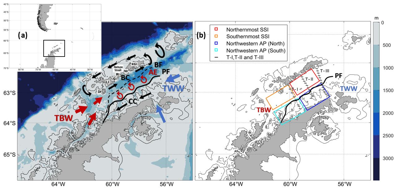
Figure 1 (a) Sketch of the circulation in the Bransfield Strait. Abbreviations for the South Shetland Islands (SSI) include DI (Deception Island), LI (Livingston Island), GI (Greenwich Island), RI (Robert Island), NI (Nelson Island) and KGI (King George Island). Abbreviations for major oceanographic features are as follows: AE (anticyclonic eddy), BC (Bransfield Current), BF (Bransfield Front), CC (Antarctic Coastal Current), PF (Peninsula Front), TBW (Transitional Bellingshausen Water) and TWW (Transitional Weddell Water). (b) Map showing cruise transects and boxes selected for dedicated analysis. The transects are from two different oceanographic cruises and include T–I and T–III from CIEMAR (December 1999) and T–II from COUPLING (January 2010). Additionally, four boxes are defined between the SSI and the Antarctic Peninsula (AP): Northernmost SSI (red), Southernmost SSI (orange), Northwestern AP (North) (dark blue) and Northwestern AP (South) (light blue). The 200 m isobath is highlighted with a black contour in both panels.

In this work, we provide a comprehensive description of the seasonal variations in chl-a concentrations in the BS, accounting for the biophysical coupling supporting their development. We hypothesize that this biophysical coupling is strongly conditioned by the spatio-temporal variability in the PF, as has been already argued.

The structure of this paper is as follows. In Sect. 2, we describe the data and methods. In Sect. 3, we present and discuss the results distributed in four subsections. In Sect. 3.1, we set our hypothesis by analysing observational data from two oceanographic cruises: CIEMAR (December 1999) and COUPLING (January 2010). In Sect. 3.2, we construct satellite-based climatologies and examine the seasonally varying horizontal distribution of SST, sea ice coverage (SIC), chl-a concentrations, wind stress and Ekman pumping. In Sect. 3.3, we present the monthly evolution of the latter variables, along with air temperature, in order to characterize the spatio-temporal variability in the bloom according to four distinct regions (Fig. 1b), which will be accounted for in the text. In Sect. 3.4, we address a review of works investigating the phytoplankton assemblage in the BS, bearing in mind the biophysical coupling previously described, in order to provide further insights based on state-of-the-art knowledge. Lastly, in Sect. 3.5, we construct satellite-based monthly climatologies of SST and chl a along the same transects sampled during the CIEMAR and COUPLING cruises to present a climatological context for our hypothesis, through which the spatial distribution of the chl-a blooms in the BS varies according to the PF (monitored via SST), which contours the hydrographic area for TBW and TWW and hosts different phytoplankton assemblages. Section 4 presents a summary of the main conclusions.

2 Data and methods

In situ observations and remotely sensed measurements are detailed in the following, separately, for clarity. Seasons are defined following Zhang et al. (2011) and Dotto et al. (2021) as summer (January–February–March), autumn (April–May–June), winter (July–August–September) and spring (October–November–December).

2.1 In situ observations: Antarctic cruises

The data inspiring the hypothesis that we address in this work, i.e. the spatial distribution of the chl-a bloom in the BS as strongly conditioned by the PF, rely to a great extent on conductivity–temperature–depth (CTD) and fluorescence measurements collected from two interdisciplinary cruises: CIEMAR and COUPLING. The fluorescence measurements were collected with an ECO fluorometer, which measures fluorescence from chl a, fDOM (fluorescent dissolved organic matter), uranine, rhodamine, and phycocyanin and phycoerythrin. In this work, we analyse the fluorescence from chl a (Hernández-León et al., 2013; Sangrà et al., 2014).

On the one hand, the CIEMAR cruise was conducted in December 1999 (Corzo et al., 2005; Primo and Vázquez, 2007; Sangrà et al., 2011), and two transects covered the region from Livingston Island and King George Island towards the northern tip of the AP. On the other hand, the COUPLING cruise was conducted in January 2010 (Hernández-León et al., 2013; Sangrà et al., 2014, 2017), and a transect covered the region from the Nelson Strait to the AP tip. Both cruises were carried out on board the R/V Hespérides. For further details about the CTD station map of both cruises, the reader is referred to Sangrà et al. (2011, 2017).

Additionally, in situ surface and subsurface (10 m depth) temperature measurements were downloaded from PANGAEA (https://www.pangaea.de/, last access: 9 March 2022) and the World Ocean Database (WOD; https://www.ncei.noaa.gov/products/world-ocean-database, last access: 25 February 2022) in order to assess the goodness of available open-access remotely sensed products of SST and support the choice of the product providing the best fit. In Table A1 of the Appendix A, a summary of the cruises and corresponding dates for the CTD measurements used is presented.

2.2 Remotely sensed products: sea surface temperature and sea ice coverage

We use satellite data of SST and SIC from the Operational Sea Surface Temperature and Sea Ice Analysis (OSTIA; Good et al., 2020) downloaded from the Copernicus Marine Environment Monitoring Service (CMEMS; https://marine.copernicus.eu/, last access: 12 March 2022) and developed by the United Kingdom Met Office. The motivation behind this choice is supported by a quantitative intercomparison between available SST open-access products and in situ temperature measurements (see this analysis in Appendix A).

OSTIA provides the SST free of diurnal variability and the sea ice concentration. It is a reprocessed dataset with a high grid resolution of 0.05°, which accounts for both in situ and satellite data and presents a processing level L4. This work analyses OSTIA data from 1998 to 2018.

2.3 Remotely sensed products: chlorophyll a

We compute monthly climatologies of surface chl-a concentrations based on multi-sensors and algorithms. The product name is OCEANCOLOUR_GLO_BGC_L4_MY_009_104, obtained from CMEMS (https://marine.copernicus.eu/, last access: 16 February 2023). The chl-a data have a spatial resolution of 4 km, a temporal range from September 1997 to the present and a processing level L4. This work analyses concentrations from 1998 to 2018.

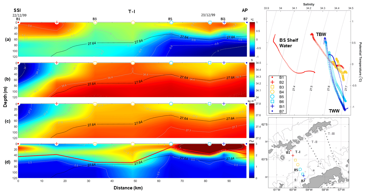
Figure 2 Vertical sections of ocean properties along transect T–I surveyed during the CIEMAR cruise (December 1999), running from Livingston Island to the Antarctic Peninsula. (a) Potential temperature, (b) salinity, (c) potential density and (d) fluorescence are shown on the left-hand-side panels. The solid black line represents the isopycnal of 27.64 kg m⁻³, used as a reference to distinguish between transitional zonal water with Bellingshausen influence (TBW) and transitional zonal water with Weddell influence (TWW; Sangrà et al., 2017). The solid red line in (d) shows the upper-mixed-layer depth computed following Holte and Talley (2009). The top right-hand-side panel displays a temperature–salinity diagram to highlight water masses: Bransfield Strait (BS) Shelf Water, TBW and TWW. Different marks and colours are displayed to represent data at each station. The bottom right-hand-side panel shows a map depicting the stations of the transect T–I.

2.4 Remotely sensed products: wind and air temperature

We use the monthly averaged reanalysis of air temperature at 2 m and wind components at 10 m from ERA5 (Hersbach et al., 2020), which have a horizontal resolution of 0.25° over the period 1940 to the present. From the wind components, we calculate the wind stress and Ekman pumping.

We calculate the wind stress (τ) and wind stress zonal (τ_x) and meridional (τ_y) components following Eqs. (1)–(3) (Patel, 2023):

$$\begin{array}{}\text{(1)}& {\displaystyle }\mathit{\tau }=\mathit{\rho }\cdot U_{\mathrm{10}}^{\mathrm{2}}\cdot C_{\text{D}},\text{(2)}& {\displaystyle }{\mathit{\tau }}_x=\mathit{\rho }\cdot U_{\mathrm{10}}\cdot u\cdot C_{\text{D}},\text{(3)}& {\displaystyle }{\mathit{\tau }}_y=\mathit{\rho }\cdot U_{\mathrm{10}}\cdot v\cdot C_{\text{D}},\end{array}$$

where ρ is the air density (1.2 kg m⁻³); $U_{\mathrm{10}}=\sqrt{u^{\mathrm{2}}+v^{\mathrm{2}}}$ is the absolute value of the wind speed at 10 m above the surface (u and v are the eastward and northward wind speed components, respectively); x and y are the eastward and northward spatial coordinates; and C_D is the drag coefficient, which is a function of wind speed, U₁₀. The equations used for wind stress computation are based on the Gill (1982) formula and a non-linear C_D based on Large and Pond (1981), modified for low wind speeds (Trenberth et al., 1990). We note that the mean C_D we obtained for our climatological maps in the BS is $\mathrm{1.4}\times {\mathrm{10}}^{-\mathrm{3}}\pm \mathrm{0.16}\times {\mathrm{10}}^{-\mathrm{3}}$, analogous to the values reported by Kara et al. (2007) over the SO.

We also compute the Ekman vertical velocity as follows:

$$\begin{array}{}\text{(4)}& w_{\text{E}}={\displaystyle \frac{\mathrm{1}}{{\mathit{\rho }}_{\mathrm{0}}}}\text{curl}\left({\displaystyle \frac{\mathit{\tau }}{f}}\right),\end{array}$$

where ρ₀ is the water density (1025 kg m⁻³) and f=2Ωsin φ is the Coriolis frequency (Ω is the Earth rotation rate, $\mathrm{7.2921}\times {\mathrm{10}}^{-\mathrm{5}}$ rad s⁻¹, and φ is the latitude). Positive (negative) w_E values indicate upward (downward) velocities leading to upwelling (downwelling).

3 Results and discussion

In this section we assess the major physical drivers potentially conditioning the vertical and horizontal structure of the chl-a bloom in the BS. To this aim, in Sect. 3.1 we analyse the vertical and horizontal structure of two chl-a blooms in the BS based on hydrographic measurements from two cruises (1999 and 2010) along three cross-strait transects (T–I, T–II, T–III). In Sect. 3.2 we analyse the seasonal variations in the horizontal structure of the chl-a bloom and the PF from a climatological perspective based on remotely sensed observations over a 21-year period (1998–2018): SST, SIC, wind stress and Ekman pumping. Next, in Sect. 3.3, we examine in detail the monthly climatologies of selected boxes of study in the BS (adding air temperature to the analysis). In Sect. 3.4, we provide a summary review of the research on the phytoplankton assemblage in the BS. Lastly, in Sect. 3.5 we construct satellite-based monthly climatologies of SST and chl a along the same locations as the transects T–I, T–II and T–III to provide a statistically robust (i.e. climatological) context to our hypothesis, through which the chl-a bloom extent varies according to the PF.

3.1 Vertical and horizontal structure along CIEMAR and COUPLING transects

We present the vertical structure of temperature, salinity, density and fluorescence in the BS (Figs. 2, 3 and 4) based on data collected during the multidisciplinary CIEMAR and COUPLING cruises in late spring 1999 and early summertime 2010, respectively. The physical oceanographic aspects from these cruises were first presented in Sangrà et al. (2011, 2017).

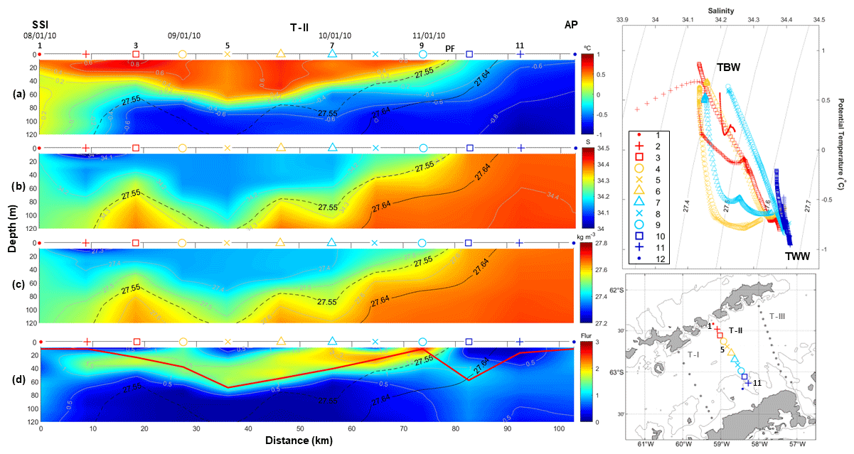
Figure 3 The same as in Fig. 2 but for T–II, surveyed during the COUPLING cruise (January 2010) and running from the Nelson Strait to the Antarctic Peninsula. Additionally, the dashed black line represents the isopycnal of 27.55 kg m⁻³, which is used as a reference more adjusted to our dataset to distinguish between TBW and TWW.

Previous studies based on these measurements are in line with biophysical phenomena focused, among other aspects, on turbulence as a driver for phytoplankton distribution as well as on mesoscale physical features as key players in determining phytoplankton assemblages (García-Muñoz et al., 2013; Macías et al., 2013; Sangrà et al., 2014). Following COUPLING cruise measurements, García-Muñoz et al. (2013) concluded that phytoplankton assemblages around the SSI were strongly connected with the Bransfield current system. Furthermore, it was suggested that, considering the recurrence of the Bransfield current system during the austral summer, the observed distribution of phytoplankton, which responded to this current system, should also be a quasi-permanent feature (García-Muñoz et al., 2013). In the following, we combine the measurements from the two cruises for the first time to address this hypothesis, where we add and highlight that the key player appears to be the cross-strait gradient marked at the surface by the PF and that this may enable the long-term monitoring of the biophysical coupling between the surface chl-a bloom and the PF based on satellite measurements.

For clarity, we name the three transects of study T–I, T–II and T–III moving from west to east. Thus, transect T–I (Fig. 2) and T–III (Fig. 4) correspond to CIEMAR and present novel measurements of fluorescence (not previously published), while transect T–II (Fig. 3), located between T–I and T–III, corresponds to COUPLING. The three transects originate over the shelf of the SSI and extend towards the AP, running nearly perpendicular to the main axis of the strait. Notably, measurements from both sea trials agree well in showing a coherent vertical and horizontal structure of hydrography and fluorescence. In Figs. 2–4, two panels are always dedicated to showing the temperature–salinity (T–S) diagram and the station map to help the reader in following the ocean property descriptions.

Starting with T–I (Fig. 2), this originates to the south of Livingston Island and extends towards the AP. Along T–I, temperatures are above 0 °C in the upper 40 m for its full extent (Fig. 2a), being relatively high in the proximity of the SSI at a distance of 0–20 km and close to the AP, where they reach near-surface values and exceed 0.6 and 0.4 °C, respectively. On the other hand, salinity is remarkably fresher and lighter near the SSI (S<34 and σ_θ<27.3 kg m⁻³), as opposed to saltier and denser waters towards the AP (S>34.3 and σ_θ∼27.6 kg m⁻³; Fig. 2b and c, respectively). Fluorescence levels exceeding 2–3 (Fig. 2d) peak in the warmest (>0.2 °C) and lightest surface waters (upper 50 m) near the SSI (stations B1–B2) and near the AP (stations B5–B7). The isopycnal of 27.64 kg m⁻³ is highlighted in black in all vertical sections as a reference to the water mass boundary between TBW (σ_θ<27.64 kg m⁻³) and TWW (σ_θ>27.64 kg m⁻³; Sangrà et al., 2011, 2017). These observations indicate the presence of relatively warm TBW flowing near the surface to the south of Livingston Island. Coastal signals of Bransfield Strait Shelf Water (BS Shelf Water), characterized by lower salinity values (Zhou et al., 2006; Polukhin et al., 2021), were also detected. In addition, relatively cold TWW flows closer to the AP at deeper levels (>60 m depth), where fluorescence sharply diminishes (<0.5) along the entire transect (Fig. 2d). The PF is not visible along T–I given the basin-wide extent of TBW at surface, which prevents shoaling of TWW.

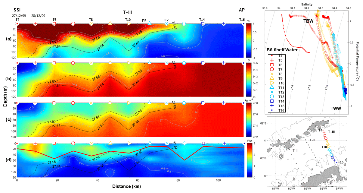
Figure 4 The same as in Fig. 2 but for T–III, surveyed during the CIEMAR cruise (December 1999) and running from King George Island to the Antarctic Peninsula. Additionally, the dashed black line represents the isopycnal of 27.55 kg m⁻³, which is used as a reference more adjusted to our dataset to distinguish between TBW and TWW.

T–II (Fig. 3) originates to the south of the Nelson Strait and extends towards the AP. Largely, along T–II, TBW is visible as warmer (Θ > −0.4 °C) and fresher (<34.45) than TWW (Sangrà et al., 2017). The subsurface signal of TWW extends towards the SSI, confronting TBW between 60–120 m depth at around stations 2–3, where they form the BF (Sangrà et al., 2011). Subsequently, the high-fluorescence patch (>1) extends within the warmest and freshest surface layers (Fig. 3d) from the surface down to 60 m depth at its deepest, contouring the isotherm of 0.2 °C from the SSI until stations 9–10. At this location, the 0.2 °C isotherm reaches the surface, temperature decreases rapidly towards the AP ($<-\mathrm{0.6}$ °C; Fig. 3a), and salinity and density increase (>34.3 and >27.64 kg m⁻³; Fig. 3b and c). This gradient forms the PF, where TBW and TWW confront each other close to the AP. Remarkably, near-surface (0–30 m) fluorescence levels decrease below 0.5 (Fig. 3d) on the TWW side of the PF.

Lastly, T–III (Fig. 4) originates to the south of King George Island and extends towards the AP. Generally, we observe an analogous vertical structure to that described for T–II, suggesting that a horizontal coherence exists between transects, especially when accounting for the fact that differences with T–I are due to the latter being at a farther distance from the Weddell Sea and, hence, presenting a weaker signal of TWW at the surface. As observed in Figs. 2 and 3, the chl-a bloom suggested by high fluorescence values (>1) is again embedded within the pool of TBW closer to the SSI, where waters are relatively warm and fresh as compared to TWW close to the AP. Moreover, the PF (stations T10–T11) appears to delimit the surface's easternmost reach of the patch with the highest fluorescence. However, we must also note that, between the PF and the AP, a less prominent and coherent patch of values higher than the baseline exists down to nearly 120 m depth, in both T–II and T–III (fluorescence > 0.5 and >1, respectively).

Remarkably, two other studies (Basterretxea and Arístegui, 1999; Gonçalves-Araujo et al., 2015) have also captured a consistent cross-strait pattern where the highest chl-a concentrations are embedded within the TBW reservoir in the first ∼60 m of the water column, and the easternmost extent of this signal coincides with the location of the PF, through which TBW and TWW interact. In both cases, in spite of the sharp decrease in chl a across the PF, chl-a concentrations were not low in the TWW reservoir and, in fact, relatively high although occupying a wider depth range (0–100 m). Their vertical sections were constructed from ship-based measurements collected along a transect parallel to T–III but farther north, departing from King George Island, in January 1993 and February–March 2009: Fig. 6 in Basterretxea and Arístegui (1999) and Fig. 3 in Gonçalves-Araujo et al. (2015), respectively. This supports the existence of different phytoplankton assemblages occupying different niches according to the dominant water masses.

In all (d) panels from Figs. 2–4, a solid red line is added to indicate UML depth (Holte and Talley, 2009). Roughly, this estimate of the UML depth fits well with the depth of the high-fluorescence patch embedded within the TBW reservoir, which keeps phytoplankton under favourable light conditions, enables a better supply of dissolved iron (Prézelin et al., 2000) and keeps phytoplankton within a depth range with proper conditions for accumulation of phytoplankton biomass (Mukhanov et al., 2021; Mendes et al., 2023). Accordingly, relatively high fluorescence (>0.5) is accumulated along the entire BS in T–I, where UML depth is relatively shallow (<60 m), especially at stations B5–B7 (fluorescence above 2 and UML depths of ∼15 m). The same pattern applies along T–II and T–III, with the high-fluorescence patch embedded within the UML. In T–II, the highest fluorescence (∼2) is located near the PF, at station 9, where the lowest UML depths occur (10 m). Similarly, in T–III a fluorescence of 2 is closer to the SSI station 2 where UML depths are around 25 m. Moreover, near the AP, relatively low UML depths (10 m) are also observed in station T14 jointly with a fluorescence of 1.

Following results in García-Muñoz et al. (2013), the fluorescence observations presented here from the COUPLING cruise (T–II in Fig. 3) can be attributed to different phytoplankton assemblages, as briefly introduced in Sect. 1, namely cryptophytes in the upper 60 m of the TBW reservoir between the BF and the PF and nanophytoplankton along the full transect but at higher abundances for the largest fraction in the TWW reservoir, accounting for the weaker but deeper signal in fluorescence (from the surface down to 100 m). This suggests that the fluorescence signal measured by the ECO fluorometer might be dominated by cryptophytes. Whether this is also the case for the CIEMAR transects (T–I and T–III in Figs. 2 and 4) is a feature we cannot confirm in the absence of a phytoplankton assemblage study for that cruise. However, a decade apart, the fluorescence distribution appears consistent in showing highest and shallower values within the relatively warm and stratified TBW reservoir, and lower but deeper values within the cold and well-mixed TWW reservoir. The stronger signal in fluorescence during CIEMAR could then be attributed to a higher abundance of cryptophytes within the TBW reservoir if we assume that the pattern observed by García-Muñoz et al. (2013) is recurrent over time. Recent studies also support this by confirming the preferred niches of cryptophytes in the BS are the relatively warm, less saline and stratified waters of the TBW reservoir, where they also compete with diatoms (Mendes et al., 2013, 2023; Gonçalves-Araujo et al., 2015; Mukhanov et al., 2021; Costa et al., 2023).

Results from the in situ measurements collected during the CIEMAR and COUPLING cruises, occurring a decade apart, plus more recent evidence of phytoplankton assemblages following the ocean dynamics of the Bransfield current system jointly further support the basis of our hypothesis: the biophysical coupling between the spatial distribution of the surface chl-a bloom and the PF in the BS may benefit from long-term monitoring using remotely sensed observations of chl a and SST.

In the following section, we analyse a set of satellite-based climatologies with the aim to demonstrate that the horizontal variability in the PF (and hence the interaction between TBW and TWW) plays a major role in determining the spatial extent of the patch with the highest surface chl-a bloom in the BS. We complete this analysis by considering the role of several physical drivers which also contribute to setting the niche for phytoplankton assemblage through a biophysical coupling. We expect this joint climatological perspective of the seasonal variations in the chl-a bloom and the PF, unprecedented in the literature, will provide the basis for their long-term monitoring. Counting on a robust long-term phytoplankton monitoring approach will enable a better understanding of the biophysical coupling that sets the baseline of the marine food web in the BS.

3.2 Seasonal variations in the chl-a bloom and Peninsula Front coupling

The remotely sensed climatologies of SST, SIC, chl a and Ekman pumping (along with wind stress) were computed for the period 1998 to 2018 and are presented in Figs. 5–8, respectively.

Regarding the SST (Fig. 5), the most outstanding feature governing the summer months in the BS is a strong cross-strait gradient, where high temperatures (>1 °C) spread around the SSI and lower temperatures (<0 °C) appear to enter into the basin from the Weddell Sea, turning around the AP and spreading southwestward along the peninsula shelf. This strong temperature gradient is the surface signal of the PF, where TBW confronts TWW. Previous studies, based on in situ summertime data, have used different thresholds for the isotherm characterizing the location of the PF at surface, where TBW and TWW interact: Sangrà et al. (2017) used the isotherm of −0.4 °C, while Catalán et al. (2008) used the isotherm of 1 °C. The choice of these isotherms is not trivial, and one must identify the isotherm embedding the waterbody flowing from the Weddell Sea into the BS, thus separating TWW from TBW. Looking at Fig. 5a, we note that the climatological isotherm characterizing the PF location at the surface during the summer months corresponds to the 0.6 °C isotherm. Through autumn and spring, the PF is also visible although a different isotherm rises as characteristic of this thermal front, being −1.2 and −0.8 °C, respectively. Lastly, during the winter months the surface signal of the PF vanishes, as one could expect, due to the atmospheric forcing prevailing in the homogenization of the upper ocean. Within the strait, surface temperatures are around −1.8 °C ± 0.2 °C.

It is worthwhile noting that in Figs. 3 and 4 we used the 0.2 and 0.8 °C isotherms, respectively, reaching the surface to define the location of the PF, and in Fig. 5 we used a different isotherm. This is not a contradiction. One must keep in mind that the 0.2 and 0.8 °C characteristic isotherms worked well through synoptic transects, which took place in late December and January, while in Fig. 5a summertime climatological field is examined after time-averaging 3 data months over a period of 21 years. This accounts for the seasonally varying values provided above, which differ from the synoptic values.

To the best of our knowledge, this is the first time that a remotely sensed SST seasonal climatology is shown with a focus on the BS. In Appendix A we present an examination of the goodness of SST satellite measurements against concomitant in situ measurements, finding that a high correlation exists between the product we use (OSTIA) and in situ measurements (R²=0.849). Also, the summertime field is in agreement with patterns reported in the literature for this season and based on in situ hydrographic measurements (Sangrà et al., 2011, 2017). Additionally, we used a recently published seasonal climatology of hydrographic properties in the BS based on in situ measurements (Dotto et al., 2021) and produced a figure (not shown) analogous to our Fig. 5 (with the same contour lines and color bar). The comparison supports the major features of the seasonal patterns described above. Exceptions occur north of the SSI in autumn and inside the BS in spring, where the abundance of mesoscale features in the climatology based on in situ measurements (Dotto et al., 2021) slightly hampers the view of the mean field pattern.

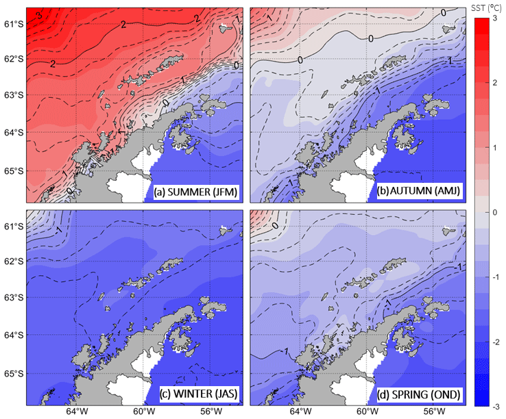
Figure 5 Seasonal maps of sea surface temperature (SST; in shades of colours) for (a) summer, (b) autumn, (c) winter and (d) spring. The capital letters between brackets stand for the initial letters of the months. The SST climatologies are averaged from January 1998 to December 2018. The dashed isotherms are plotted at intervals of 0.2 °C, while the solid lines mark each 1 °C interval.

Figure 6 shows the seasonal SIC as a percentage of area covered by sea ice. A value of SIC of about 15 % is taken as indicative of the presence of sea ice. Thus, during the summer and spring months, the BS is generally free of sea ice with SIC <15 %. Through autumn, the atmospheric forcing starts leading the development of the SIC in the BS, which extends firstly over the colder waters of the Weddell Sea intrusion with SIC ranging from 15 % to 25 % (compare Figs. 5b and 6b). This is in agreement with a recent study developed over the western AP, which addresses the role of subsurface ocean heat in the modulation of the sea ice seasonality and highlights the importance of the upper-ocean variability in setting sea ice concentrations and thickness (Saenz et al., 2023). Towards winter, the SIC is greater than 25 % everywhere in the BS (Fig. 6c), promoted by near-freezing sea surface temperatures of around −1.8 °C ± 0.2 °C (Fig. 5c).

Taking into account the fact that the seasonal sea ice retreat is complete from spring to summer in the entire BS suggests that the larger freshwater inputs reported in the literature over the TBW domain and contributing to the vertical stabilization of the water column might be driven by a warmer oceanic forcing over coastal and glacial areas (Cook et al., 2016) rather than by melting of the open-ocean sea ice.

Figure 6 The same as Fig. 5 but for sea ice coverage (SIC). Solid black lines indicate a SIC percentage of 15 %, which is the threshold for considering the presence of sea ice significant. Dashed grey lines represent SIC percentages of 25 %, 50 % and 75 %.

Following seasonal panels in Fig. 7, the development of the chl-a bloom in the BS is particularly revealing when using a logarithmic scale, which highlights spatial patterns that are otherwise slightly masked due to the strong signal of chl a east of the AP in the Weddell Sea. West of the AP, chl-a bloom concentrations have been reported to range normally between 0.5–1 mg m⁻³ (Ducklow et al., 2008; Smith et al., 2008). However, we must note that this threshold varies significantly depending on the study region given that there are areas with naturally either higher or lower phytoplankton concentrations.

Generally speaking, the chl-a bloom in the BS starts developing in spring, reaching its maximum horizontal extent with values above 0.5 mg m⁻³ during the summer months and still presenting patchy regions of high chl a during autumn (Fig. 7). We find that in the BS the isoline of 0.5 mg m⁻³ works well as the threshold contouring the chl-a bloom around the SSI, as this appears to embed coherently in space the region with the highest chl-a values during the summer months. Through winter, surface chl-a concentrations drop below 0.25 mg m⁻³ everywhere in the BS except for the region adjacent to the northern shelf of the westernmost SSI (>0.25 mg m⁻³). We observe that although the BS receives inflows from the Weddell Sea to the east of the AP, the much higher chl-a concentrations present in the Weddell Sea do not extend into the BS. This is in spite of the fact that the waters from the Weddell Sea are continuously propagating around the northern tip of the peninsula and entering the BS. Notably, this feature persists year-round and the chl-a bloom never develops in the climatologies covering at its highest values the entire BS. Differently, at its largest extent, with values higher than 0.5 mg m⁻³ (summer months), the chl-a bloom appears constrained to the domain of TBW sourced from the Bellingshausen Sea, while the presence of TWW marks the boundary where chl-a concentrations drop sharply within the BS. By comparison between Figs. 5a and 7a, it becomes evident that the spatial extent of the surface chl-a bloom surrounding the SSI (chl a >0.5 mg m⁻³) aligns well with the surface signal of the PF in the BS, where TBW and TWW confront each other. To ease visualization of this coupling, the isotherms of 1 and 0.6 °C have been added over the summertime chl-a field (Fig. 7a).

This bloom area where chl-a concentrations are higher than 0.5 mg m⁻³ coincides in the cross-strait direction with the chl-a bloom boundaries reported by García-Muñoz et al. (2013) for cryptophytes and large nanophytoplankton surrounding the SSI (their Fig. 4). On the Drake Passage side, the oceanward extent of their bloom ended at the subsurface Shetland Front (García-Muñoz et al., 2013), embedding TBW over the northern shelf of the SSI and accounting for the recirculation of TBW around the archipelago driven by the Bransfield Current (Sangrà et al., 2017). In Fig. 5a, the alignment of the subsurface Shetland Front to the north of the SSI is suggested by the isotherm of 1.6 °C, which roughly follows the oceanward extent of the surface chl-a bloom (Fig. 7a). On the BS side, the chl-a bloom investigated in García-Muñoz et al. (2013) also transitioned towards lower values across the PF in agreement with this study (Figs. 5a and 7a) and previous and later works (Basterretxea and Arístegui, 1999; Mendes et al., 2013; Gonçalves-Araujo et al., 2015; Mukhanov et al., 2021). Lastly, we also note the resemblance of our summertime satellite-based climatologies of SST and chl a (Figs. 5 and 7) with those based on 18 years of summertime hydrographic and chl-a measurements, through which Hewes et al. (2009) demonstrate that the distribution of high chl a around the SSI corresponded to shallow UML depths in iron-rich waters at salinities ∼34 (their Fig. 4).

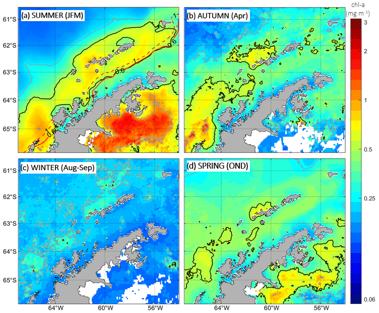
Figure 7 The same as Fig. 5 but for chlorophyll-a (chl-a) concentrations. Solid black lines indicate chl-a concentrations of 0.5 mg m⁻³, while solid grey lines represent chl-a concentrations of 0.25 and 1 mg m⁻³. Solid and dashed red lines in (a) indicate 0.6 °C and 1 °C summer isotherms, respectively (see Fig. 5a). For the autumn season (b), only the mean of April is considered due to the absence of data during other months, which results from the presence of ice cover. Similarly, for the winter season (c), the mean of August and September are solely considered for the same reason.

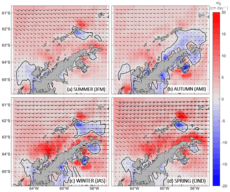
Figure 8 The same as Fig. 5 but for Ekman pumping. Positive (negative) vertical velocities are indicated in shades of red (blue) and represent upwelling (downwelling) processes. Solid black lines refer to zero velocities. Solid red and blue lines represent vertical velocities of 10 and −10 cm d⁻¹, respectively. Black vectors depict the wind stress. The wind stress reference vector is displayed over the southern AP with a value of 0.02 N m⁻².

In Fig. 8, the seasonal climatology of the wind forcing acting over the bloom domain is presented following the wind stress field (black vectors) and Ekman pumping (vertical velocity; w_E). The dominant winds in the BS are the westerlies (Vorrath et al., 2020), which flow across the strait with greater basin-wide intensity during winter and spring months. In shades of colours, the Ekman pumping is shown with positive (red) and negative (blue) vertical velocity values, implying that wind stress drives either local upwelling or local downwelling, respectively. Generally, upwelling is observed in the BS throughout the year, with a few spatial and temporal exceptions. Downwelling occurs mostly south of King George Island year-round. During autumn, this downwelling area south of King George Island expands towards the AP more extensively. This feature remains through the winter months, although it is constrained to a smaller extent that does not reach the AP. During winter and spring, the westerlies drive relatively strong upwelling vertical velocities in the BS, especially along the shelf west of the AP.

Importantly, during spring and summer (months of chl-a development; Fig. 7a and d), the westerlies appear slightly stronger along the southern shelf of the SSI (over the domain of TBW) as compared to westerlies acting over the shelf west of the AP (over the domain of TWW). Following this, one could reasonably expect deeper mixed layers over the domain where the wind stress forcing is stronger; however, along the southern shelf of the SSI, winds favour the Bransfield Current transport of TBW via downwelling-favourable Ekman transport while, along the shelf west of the AP, winds exert a moderate counterforcing to the entrance of the Antarctic Coastal Current driving upwelling-favourable Ekman transport. We find that this asymmetry may be contributing to maintaining the two distinct niches across the PF: warmer, less saline and stratified waters transported by the Bransfield Current on the TBW side and colder, saltier and well-mixed waters transported by the Antarctic Coastal Current on the TWW side.

3.3 Monthly variations in the chl-a bloom and Peninsula Front coupling

Following results from previous subsections, we note that two areas in the BS are distinctive, not only regarding their ocean dynamics as previously known (Fig. 1), but also regarding the nature of the chl-a bloom. The first one is where the chl-a bloom spreads with the highest concentrations over the relatively warm and more stratified TBW, flowing northeastward along the southern shelf of the SSI. The second one is the relatively cold and more homogeneous TWW flowing southwestward along the western shelf of the AP.

For further study of the monthly evolution of ocean and atmospheric conditions influencing the development of the surface chl-a bloom over each area, we divided the BS into four boxes of study (Fig. 1b). These boxes were designed to capture, respectively, the northern and southern domain of the surface chl-a bloom embedded in TBW south of the SSI and northern and southern domain of the surface chl-a bloom embedded in TWW west of the AP. The resulting climatologies of SST, air temperature, SIC, chl a, along-shore wind stress and Ekman pumping over the period 1998–2018 are presented in Fig. 9 and reveal several spatio-temporal similarities, and differences, which stand out and provide further insights. To this aim, the wind stress was decomposed into its along-shore (${\mathit{\tau }}_{x^{\prime }})$ and cross-shore (${\mathit{\tau }}_{y^{\prime }})$ components through rotation of the Cartesian components by 36.25° in an anti-clockwise sense.

The monthly climatologies of SST and air temperature (Fig. 9a and b) present a coherent seasonal cycle where warmer (colder) temperatures are found within all the regions for the summer (winter) months. Spatially, SSTs within the boxes south of the SSI are generally warmer than those along the western AP. This is more prominent during the summer months, when cross-strait temperature gradients are higher with differences between boxes at opposite ends of the strait of about 0.6 to 1.4 °C (Fig. 9a). These differences decrease approaching the winter months, when all regions at the surface approach near-freezing temperatures of about −1.8 °C from July to August. Evolving through the spring months, temperature differences start to increase again but are not higher than 1 °C when comparing boxes along the southern shelf of the SSI and along the shelf of the AP. Because boxes south of the SSI, sourced by TBW, depart from higher temperatures and all regions reach near-freezing temperatures during winter, their seasonal amplitudes are larger (and the slopes are more pronounced) as compared to boxes along the shelf of the western AP, sourced by TWW. Thus, the seasonal amplitude of the SST is more than 1.5 times larger for the southern shelf of the SSI (∼3 °C) than along the western AP shelf (∼1.8 °C).

The seasonal amplitude of the air temperature cycle (Fig. 9b) is larger than that displayed in SST. However, warmer temperatures are once again observed in the boxes situated along the southern shelf of the SSI, where temperatures evolve from 1 °C (summer) towards −5 to −6 °C (winter), in contrast to the boxes situated along the western AP shelf, where temperatures evolve from 0 °C (summer) towards −8 °C (winter). As compared to the SST annual cycle, we observe the air temperature is more homogeneous during the summer and spring months (temperature differences among boxes are <1.25 °C) than during autumn and winter (temperature differences among boxes are >2.5 °C). This is the reverse pattern to that shown for SST, where more homogeneous temperatures among regions were found through the winter months. The reason behind the more homogeneous pattern in SST during the winter months may be due to seawater approaching near-freezing temperatures, which sets a threshold that homogenizes the ocean surface under an extreme-cooling atmospheric forcing.

The SIC monthly climatology (Fig. 9c) follows an inverse relationship with SST and air temperature (Fig. 9a and b), where higher values of SIC are found during the late-autumn, winter and early-spring months and an absence of sea ice is found through late-spring, summer and early-autumn months (<15 % SIC). Through these latter seasons, the sea ice retreat drives melting waters into the environment. This is a key factor in phytoplankton biomass accumulation, since it allows upper-ocean stratification during spring–summer, leading to favourable sunlight conditions for phytoplankton to grow (Ducklow et al., 2013). Then, the SIC peaks in July at about 50 % closest to the AP tip and at about 40 % farther south along the AP and south of the northernmost SSI. A month later the SIC peaks in August at about 30 % south of the southernmost SSI.

Remotely sensed chl-a observations enable the visualization of the monthly evolution from August to April (Fig. 9d) with a data gap due to sea ice coverage from May to July. Yet, a seasonal cycle is visible with higher chl-a concentrations through the spring and summer months, lower and declining chl-a concentrations through early autumn, and lower and increasing chl-a concentrations through late winter. This latter increasing trend is concomitant with the decrease in SIC, when sea ice starts melting in August (the same month as when SST and air temperature also start increasing). Following the literature, the date of the bloom initiation is determined as the first day at which chlorophyll levels rise to 5 % above the climatological median (Siegel et al., 2002) and stay above this value for at least 2 consecutive weeks (Thomalla et al., 2011). This threshold was computed assuming linear interpolation over winter to obtain the climatological median. Bearing these criteria in mind, our climatologies indicate that the chl-a bloom in the BS starts in mid-October, departing from a baseline for chl-a concentrations of ∼0.2 mg m⁻³ in August. From mid-October (early spring) onwards, chl-a concentrations start increasing in the entire BS, although more steeply along the southern shelf of the SSI, and are slightly delayed in the northern box of the western shelf of the AP.

The chl a peaks through December and February at 0.68 mg m⁻³ south of the southernmost SSI and in February at 0.63 mg m⁻³ south of the northernmost SSI (Fig. 9d). Along the shelf of the western AP, chl a peaks to the south in December at 0.43 mg m⁻³ and, 1 month later, to the north in January at 0.37 mg m⁻³. Generally, although standard deviations are large and overlap each other's cycles, these monthly climatologies suggest a northward development for the chl a peaks with about 1–2 months of delay.

The pattern described above for the four boxes of study supports the likely existence of two different chl-a blooms that develop simultaneously but are of a different nature (i.e. phytoplankton assemblage) in the BS, as suggested by their different intensities and timings (month of initiation and rate of increase). This is in agreement with former results in a series of studies which reported that cryptophytes compete in the BS primarily with diatoms and other nanophytoplankton groups (Mura et al., 1995; García-Muñoz et al., 2013; Mendes et al., 2013, 2023; Gonçalves-Araujo et al., 2015; Mukhanov et al., 2021; Costa et al., 2023), following strategies to adapt better to water mass distribution in the basin, which ultimately controls the time and space variability in BS phytoplankton communities.

Only two former studies have reported monthly climatologies of the surface chl-a bloom in the BS; however, neither of them framed the boxes of study such that the two blooms were simultaneously, and distinctively, captured. In the first study, Gonçalves-Araujo et al. (2015) placed a rectangular box embedding both margins of the BS at the same time, with no distinction between the TBW and TWW domains. The resulting time series (2002–2010) displays a strong interannual variability, with summertime values ranging from ∼1.1 mg m⁻³ (2006) to 0.37 mg m⁻³ (2003; their Fig. 9). In the second study, La et al. (2019) placed a slanted rectangular box parallel to the SSI coastline and similar to our two boxes south of the SSI, but in their case it extended towards Elephant Island. The resulting monthly climatology of the chl a over the period 2002–2014 (12-year mean) displays the cycle from October to April. The chl-a bloom then develops from baseline concentrations below 0.2 mg m⁻³ in October to peak concentrations ranging from ∼1.75–1.95 mg m⁻³ (their Fig. 2) through February to March. We attribute the higher climatological values in La et al. (2019), occurring about 1 month later than in our boxes along the SSI, to the different choice of the study area. In their case the northward extension of the box may be including dynamics out of the BS, from the confluence zone with the Weddell Sea. Also, the latter peak in time for this extended region is in agreement with our results in Fig. 9d, which suggests the maxima in chl a develop later as one moves northward along the BS.

Finally, the along-shore wind stress (Fig. 9e) displays year-round downwelling-favourable winds along the southern shelf of the SSI and upwelling-favourable winds along the shelf of the western AP. In all cases, a quarterly cycle stands out with maximum values (in descending order) in September, December, February and May (i.e. winter, spring, summer and autumn). A similar cycle is found along the shelf of the western AP for the Ekman pumping (Fig. 9f), where vertical velocities are upwelling favourable (positive) year-round with a quarterly cycle (same maximum time variability). Along the southern shelf of the SSI, vertical velocities are also upwelling favourable (positive) year-round but less intense and more homogeneous through the seasons. Peak vertical velocities are 20, 17.5 and 5 cm d⁻¹ for boxes along the shelf of the western AP, south of the southernmost SSI and south of the northernmost SSI, respectively.

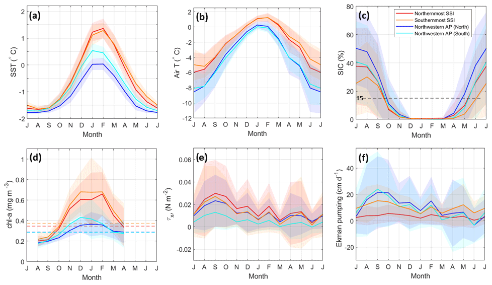
Figure 9 Monthly climatology over the period 1998 to 2018 of (a) sea surface temperature (SST), (b) air temperature, (c) sea ice coverage (SIC), (d) chlorophyll-a (chl-a) concentration, (e) along-shore wind stress and (f) Ekman pumping (vertical velocity) for each study box, as delimited in Fig. 1b. The horizontal dashed line in (c) indicates the threshold (15 %) to consider significant the presence of sea ice, while horizontal dashed lines in (d) indicate the threshold set to identify the initiation of the bloom following Siegel et al. (2002) and Thomalla et al. (2011). The mean monthly values are represented by solid lines, while the corresponding standard deviation is shown in coloured shades.

3.4 Spring–summertime phytoplankton assemblages of the chl-a bloom: historical observations

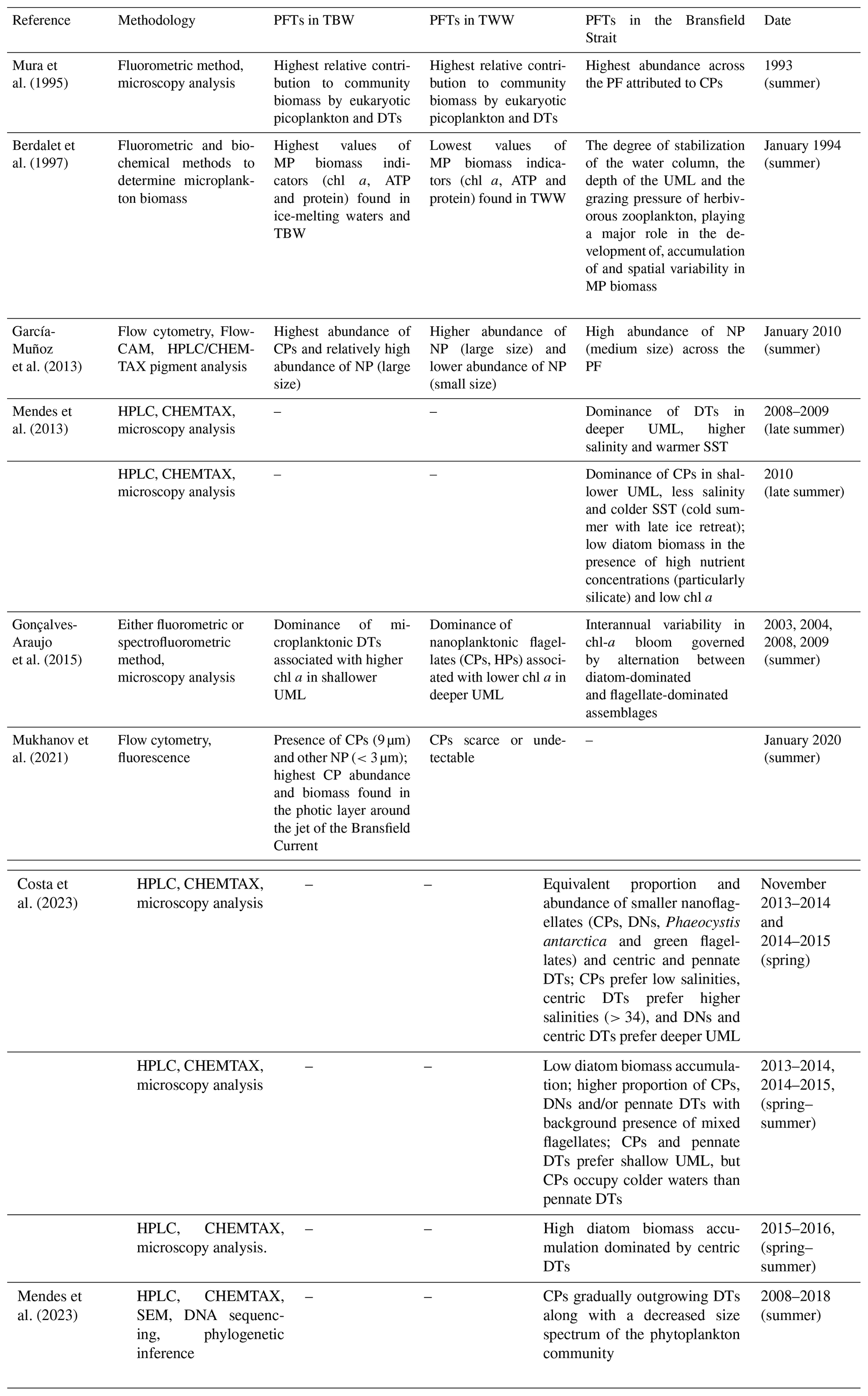
Through the previous section, we have learned that a proper design of study boxes aligned with the climatological summertime position of the PF enables the identification of two distinct chl-a blooms in the BS based on satellite measurements according to two water mass scenarios: TBW and TWW. In this section, we review more than 3 decades of previous studies and indicate their main findings in Table 1 so that we can discuss them thoroughly and identify common patterns observed in the past.

In summary, existing observations listed in Table 1 support the claim that the phytoplankton community in the BS responds to a variety of factors which may vary from year to year, thus introducing high interannual variability into the phytoplankton assemblage. The factors primarily driving the nature of the chl-a bloom are (1) the vertical stability of the water column; (2) the depth of the UML, which influences the penetration of light into the depth range where biomass may accumulate near the surface; (3) the existence of sea ice retreat, supplying relatively cold freshwater to the environment; and (4) the grazing pressure of herbivorous zooplankton. Berdalet et al. (1997) already accounted for these four factors and reported that the combination of them appears to play a major role in the development of, accumulation of and spatial variability in microplankton biomass. After reviewing the most recent studies, we confirm this statement still holds in water and also applies to at least the nanophytoplankton size (there is a scarcity of works investigating picophytoplankton along cross-strait transects in the BS, so we cannot extend the statement robustly to this phytoplankton size). Interestingly, these physical factors may also condition the phytoplankton succession through a given bloom season, and, thus, small cells appear to dominate the phytoplankton community structure during spring as large cells develop to form blooms in summer months (Petrou et al., 2016).

In this context, it is worthwhile highlighting the results from two studies employing multi-year datasets of in situ observations of phytoplankton assemblage in the BS through four (Gonçalves-Araujo et al., 2015) and nine (Mendes et al., 2023) different bloom seasons.

On the one hand, in the first study, Gonçalves-Araujo et al. (2015) investigated microplankton (20–200 µm) and nanoplankton (2–20 µm) during the summertime periods of 2003, 2004, 2008 and 2009, identifying three main taxonomic groups within the study area: diatoms, flagellates and cryptophytes. From year to year, the surface distribution of phytoplankton size was dominated by nanoplankton in 2003, 2004 and 2008 (>80 % of the total chl a) with no clear cross-strait gradient. Differently, in 2009 the surface distribution of chl a presented two distinct domains: (1) in the TBW pool, a mixed community of microplankton and nanoplankton at high (∼50 %–70 %) and low (∼30 %–50 %) percentages of the total chl a and (2) in the TWW pool, a reversed mixed community of nanoplankton and microplankton at high (∼80 %) and low (∼20 %) percentages of the total chl a. Regarding the taxonomic groups, Gonçalves-Araujo et al. (2015) found that interannual variability in species composition resulted from an alternation between diatom-dominated and flagellate-dominated assemblages: 2003 and 2004 were dominated by cryptophytes nearly everywhere in the BS, 2008 by flagellates, and 2009 by a mixture of diatoms close to the SSI and flagellates close to the AP.

Interestingly, in the second study, Mendes et al. (2023) investigated a subsequent period of time (2008–2018) based on measurements from nine different years (2011 and 2012 are absent) and demonstrated a strong coupling between biomass accumulation of cryptophytes, summer upper-ocean stability and the mixed layer. For 2008–2018, Mendes et al. (2023) reported that cryptophytes present a competitive advantage in environments with significant light level fluctuations, normally found in confined stratified upper layers, and supported that observational finding with laboratory experiments where cryptophytes revealed a high flexibility to grow in different light conditions driven by a fast photo-regulating response. These results provided the basis for understanding why the environmental conditions promoted the success of cryptophytes in coastal regions, particularly in shallower mixed layers associated with lower diatom biomass, and highlighted a distinct competition or niche separation between diatoms and cryptophytes. Regarding long-term variability, Mendes et al. (2023) concluded that cryptophytes are gradually outgrowing diatoms along with a decreased size spectrum of the phytoplankton community. This is in agreement with recent results indicating that the increasing meltwater input in the BS can potentially increase the spatial and temporal extent of cryptophytes (Mukhanov et al., 2021), which benefit from the higher stabilization of the water column driven by freshwater input.

This reported shift towards a higher abundance of cryptophytes over diatoms is not trivial and, if it persists in time, will eventually impact the biogeochemical cycling in Antarctic coastal waters due to a shift in trophic processes (Mukhanov et al., 2021). The latter work poses the scenario as follows. The replacement of large diatoms with small cryptophytes favours consumers like salps over Antarctic krill. Salps, a food competitor of Antarctic krill, can feed on a wide range of taxonomic and size compositions of phytoplankton prey. Thus, salps present a much lower feeding selectivity (Haberman et al., 2003) than Antarctic krill, which present positive selectivity for diatoms (large prey) and avoid cryptophytes (smaller prey) when feeding on complex prey mixture (Haberman et al., 2003). The shift towards an increasing role of cryptophytes in BS waters would then lead to constraints in food supply for krill, strengthening the abundance of its competitor. This would threaten not only Antarctic krill populations, but also higher consumers, including penguins, seals and whales, which feed on krill (Loeb et al., 1997).

Based on the above discussion, we find that the biophysical coupling between the chl-a blooms on both sides of the PF is largely the result of interannually varying physical properties determined by the TBW and TWW pools and that some of those physical properties could be easily monitored via remotely sensed observations such as (1) SST to track the extent of the TBW and TWW pools and (2) SIC to monitor the sea ice budget and sea ice retreat as an indication of vertical stability for the water column. Through the last section of this study before the Conclusions, we attempt to highlight the claim that monitoring the spatio-temporal distribution of the chl-a blooms in the BS according to satellite measurements of SST and chl a may offer pivotal knowledge in future studies about the potential factors driving the long-term variability in the phytoplankton assemblage across the PF.

Table 1 Historical observations investigating the chlorophyll-a bloom in the Bransfield Strait and reporting a description of the phytoplankton assemblage either by water mass domain (TBW or TWW) or without distinction. We must note that in none of the studies is the full spectrum of phytoplankton functional types (PFTs) covered, and so this review attempts to provide a general overview of existing knowledge. Abbreviations for PFT sizes are as follows: microphytoplankton (MP; 20–200 µm), nanophytoplankton (NP; 2–20 µm) and picophytoplankton (PP; 0.2–2 µm). Other abbreviations for PFTs are diatoms (DTs), cryptophytes (CPs), haptophytes (HPs) and dinoflagellates (DNs). Lastly, abbreviations for methodology are high-performance liquid chromatography (HPLC), chemical taxonomy (CHEMTAX) software v1.95 (Mackey et al., 1996) and scanning electron microscopy (SEM).

3.5 Monthly variations in SST and chl a along the CIEMAR and COUPLING transects

As closure to our analyses, we return to the synoptic transects which motivated our hypothesis, based on in situ hydrographic and fluorescence measurements (T–I, T–II and T–III; Figs. 2–4), and construct spatio-temporal climatologies of remotely sensed SST and chl a along the same transects (for reference, a series of black dots denote the spatio-temporal position of the hydrographic stations in the Hovmöller diagrams in Fig. 10). The aim is to highlight that the monthly variability in the easternmost extent of the chl-a bloom in the TBW pool and the westernmost extent of the chl-a bloom in the TWW pool responds closely to the monthly variability in the PF. We think this approach further supports the potential of long-term monitoring of the observed biophysical coupling via remotely sensed measurements when study boxes are properly placed according to governing ocean dynamics.

From early spring (October) to early autumn (April), the PF emerges prominently along transects T–II and T–III (Fig. 10a), where relatively warm TBW, richer in chl a along the southern shelf of the SSI (SST >1.4 °C; chl a∼0.7–0.8 mg m⁻³), opposes relatively cold TWW that is poorer in chl a (SST $\sim -\mathrm{0.2}$ to −0.6 °C and chl a <0.3–0.4 mg m⁻³) along the western shelf of the AP (Fig. 10b).

It is worthwhile noting that the PF delineated along the synoptic transect T–II, found between stations 9–10 (Fig. 3), corresponds closely to the climatological location of the PF (0.6 °C and 0.5 mg m⁻³) observed between stations 8–9 (Fig. 10a). Similarly, along T–III, both the hydrographic PF and the climatological PF are found at the same position, between stations T10 and T11.

As it occurred along the synoptic transect T–I (Fig. 2), the PF is not visible along the climatological transect T–I (Fig. 10a), where relatively warm TBW invades the strait, and the TWW signal is absent from early spring (October) to early autumn (April) with SST values ∼0.2 °C. The absence of a strong cross-strait temperature gradient along T–I is in agreement with an elongated patch of high chl-a concentrations which expands towards the western shelf of the AP, reaching values of ∼0.5 mg m⁻³ as far east as 84 km offshore the SSI (Fig. 10b). This is analogous to the basin-wide high fluorescence signal shown along the synoptic transect T–I in Fig. 2.

Throughout the remainder of the year, both SST and chl-a values follow similar patterns along the three climatological transects (T–I, T–II and T–III), displaying basin-wide, lower and more homogeneous values.

Notably, the highest chl-a concentrations are always found offshore along the three climatological transects, embedded in patches of the warmest TBW (SST >1.2–1.4 °C; chl a ∼0.6–0.8 mg m⁻³). These climatological transects (Fig. 10b) confirm an earlier suggestion based on Fig. 9, where the northward spatio-temporal migration of the chl-a bloom is apparent. Here we note that the highest chl-a concentrations along the three climatological transects occur around December in T–I, in December to February in T–II and around February in T–III.

In summary, the remotely sensed observations of SST and chl-a concentrations have proven to be of great potential in the monitoring of major features of the chl-a blooms in the BS, accounting for a biophysical coupling between two hydrographic scenarios (TBW and TWW pools) that confront each other along the PF. Importantly, we recall that these two hydrographic scenarios embed different phytoplankton assemblages, as has been discussed based on previous literature and results from this study.

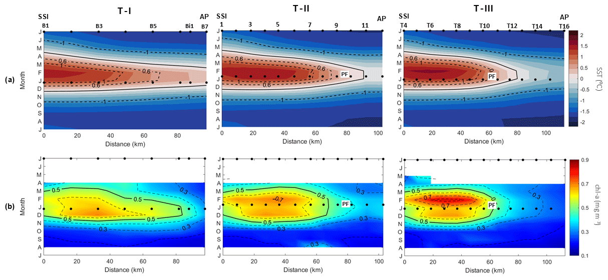
Figure 10 Monthly climatology from 1998 to 2018 of (a) sea surface temperature (SST) and (b) chlorophyll-a (chl-a) concentration for each study transect (see Figs. 2–4) from the South Shetland Islands (SSI) to the Antarctic Peninsula (AP). The black markers (dots) situated at the top of the subplots represent the stations' positions along the transects. These same stations are also displayed during the summer months when the cruises were carried out. Additionally, the position of the Peninsula Front (PF), as identified during the cruises and located along the isopycnal of 27.55 kg m⁻³, is also indicated.

Lastly, it is worthwhile noting that the alignment of the chl-a spatial distribution along an oceanic front is not a novel feature in the world's oceans and has already been investigated in the literature (Moore and Abbott, 2002; Baird et al., 2008; Von Bodungen et al., 2008). Thus, the novelty of our work lies in demonstrating through in situ observations and remotely sensed measurements that such a biophysical coupling has the potential to be used to monitor the chl-a blooms and phytoplankton assemblages occurring seasonally in the BS. This aspect is particularly relevant because the BS is a key region for the sustainability of Antarctic marine ecosystem, which is challenging to monitor due to the hazardous prevailing conditions in polar regions. In future studies, we expect the calculation of the frontal probability (Yang et al., 2023) of the PF through a multi-year time series of SST data may be beneficial for interannually assessing and co-locating the alignment of the thermal front and the chl-a bloom domains using an automated algorithm for the Bransfield Strait study case (see Appendix B for further insights).

4 Conclusions

In this study, we address the hypothesis that the spring-to-summertime biophysical coupling controlling the chl-a bloom in the BS could be monitored through a combination of remotely sensed observations of chl a and SST, which strongly condition the spatio-temporal variability in the phytoplankton assemblage across the PF. Our approach is based on the characterization of climatological fields, following a motivation driven by novel and historical synoptic in situ observations which reveal that the PF may be used as a guideline to contour two distinctive niches for phytoplankton assemblage in the BS, both horizontally and vertically.

Based on remotely sensed climatologies, we find that the surface distribution of the seasonal variation in the SST and chl a in the BS enables the identification of two environmentally different scenarios for phytoplankton, which then grow under different strategies according to the revised literature.

The first scenario is the pool of Transitional Bellingshausen Water, relatively warm and less saline waters in a stratified water column with shallow mixed layers as compared to the second scenario. The second scenario is the pool of Transitional Weddell Water, relatively cold and more saline waters in a well-mixed water column with deeper mixed layers. We find that the climatological isotherm characterizing the PF location at the surface during the summer months corresponds to the 0.6 °C isotherm, which divides the BS in two domains. This division is further supported when we show that the isoline of 0.5 mg m⁻³ concentration of chl a aligns with the 0.6 °C isotherm, which works well as a threshold contouring the chl-a bloom around the SSI and coherently embedding in space the region with the highest chl-a values during the summer months.

Following the seasonal climatology of the SIC, we notice that the larger freshwater inputs reported in the literature over the TBW domain and contributing to the vertical stabilization of the water column might be driven by a warmer oceanic forcing over coastal and glacial areas of the SSI (Cook et al., 2016; Saenz et al., 2023) rather than by melting of the open-ocean sea ice. On the other hand, the seasonal climatology of the wind stress forcing suggests that the westerlies may play a major role in contributing to (1) stratified waters in the TBW domain via downwelling-favourable Ekman transport along the southern SSI shelf, through which the Bransfield Current flows, and (2) well-mixed upper layers in the TWW domain via upwelling-favourable Ekman transport along the western AP shelf.

Moreover, based on ad hoc study boxes located according to the spatial distribution of the remotely sensed chl-a concentrations, we conclude that two different climatological chl-a blooms that develop simultaneously but are of a different nature (i.e. phytoplankton assemblage) can be identified in the BS, as suggested by their different intensities and timings (month of initiation and rate of increase). This is in agreement with former results in a series of studies which reported that cryptophytes compete in the BS, primarily with diatoms and other nanophytoplankton groups (Mura et al.; 1995; García-Muñoz et al., 2013; Mendes et al., 2013, 2023; Gonçalves-Araujo et al., 2015; Mukhanov et al., 2021; Costa et al., 2023), following strategies to adapt better to the physical environment present throughout that year and which were displayed differently by zones in the monthly climatologies of SST, air temperature, SIC and wind stress forcing. Generally speaking, these studies have reported that TBW chl-a concentrations are commonly characterized by cryptophytes and small diatoms, while TWW chl-a concentrations are more frequently characterized by large diatoms.

We also note that the biophysical coupling between the chl-a blooms on both sides of the PF is largely the result of interannually varying physical properties determined by the TBW and TWW pools, as we revisit our results and compare them against the existing literature on phytoplankton assemblage in the BS. This suggests that the combined analysis of remotely sensed observations of chl a and SST (as presented in this study) may be of help in elucidating the spatio-temporal variability in the two blooms that occur in the BS during the summer months from year to year. Nevertheless, we must note that a given uncertainty will still exist when it comes to knowing which phytoplankton community may dominate the TBW and the TWW pools from year to year, unless existing remotely sensed phytoplankton assemblage products are further validated in the future. We have explored such products (not shown), but the lack of a product detecting only cryptophytes hampers the assessment of their year-to-year competition with diatoms (for which a product actually exists) in the BS. We assert that this would be of paramount importance for a more comprehensive understanding of the marine ecosystem composition in the BS.

Lastly, we conclude that combined analyses of remotely sensed observations of SST and chl-a concentrations have great potential to capture major features of the chl-a blooms in the BS, accounting for a biophysical coupling between two hydrographic scenarios (TBW and TWW pools) that confronted each other along and across the PF. We think that these results highlight the importance of long-term monitoring of the spatio-temporal distribution of the chl-a blooms in the BS using satellite measurements of SST and chl a. Such monitoring may prove pivotal for future studies investigating the forcings driving the long-term variability in the phytoplankton assemblage in the BS.

Appendix A: Assessment of the SST products

We assess the goodness of three available SST products by comparison with near-surface (0–1 and 10 m depth) in situ temperature measurements collected from a variety of Antarctic cruises (Table A1). By linear regression, the coefficient of determination (R²) is used to evaluate the performance of the three satellite products, which are (1) Optimum Interpolation SST (OI SST; https://www.remss.com/, last access: 10 March 2022), (2) the European Space Agency Climate Change Initiative (ESA CCI; https://marine.copernicus.eu/, last access: 12 March 2022), and (3) Operational Sea Surface Temperature and Sea Ice Analysis (OSTIA; https://marine.copernicus.eu/, last access: 12 March 2022). For brevity, hereafter, we refer to them as OI SST, ESA CCI and OSTIA, respectively.

The grid spacing for OI SST is ∼0.1°, but for both ESA CCI and OSTIA it is 0.05°. Meanwhile, their temporal extents are also different: the OI SST time range is from 1 June 2002 to the present, ESA CCI time range is from 1 September 1981 to 31 December 2016 and the OSTIA time range is from 1 October 1981 to 31 May 2022.

For a fair comparison, because the OI SST product starts globally in 2002, we first compare the three products to the GOAL (GOAL03, GOAL04 and GOAL05) and BREDDIES (2003) cruises at two different depths (0–1 and 10 m; see Table A2 to learn about the number of profiles by depth level used in the analysis, and Table A3 to learn about the results). Based on the low coefficients found for OI SST as compared to ESA CCI and OSTIA (Table A3), we decide to discard OI SST for further analysis.

Lastly, we use the entire dataset of available hydrographic observations (Table A1) in the study region, making a distinction between whether we use only data falling within the Bransfield Strait (BS), the Gerlache Strait (GS) or both (full domain). These data are summarized in Table A4, where there are indications of the depth levels involved in the analysis: 0–1 m (8 cruises with 539 stations from 1990 to 2010) and 10 m (21 cruises with 1133 stations from 1990 to 2011).

Results in Table A5 show the lowest coefficients are found in the Gerlache Strait for both ESA CCI and OSTIA, while these values increase when including measurements from the Bransfield Strait. To some extent, this agrees with the expectation caused by the narrow nature of the Gerlache Strait (∼10 km at its narrowest part and ∼50 km at its widest part). This implies the ocean in the Gerlache Strait is in close proximity to land nearly everywhere, leading to the discrepancies between remotely sensed and in situ observations (Zhang et al., 2004; Xie et al., 2008; Lee and Park, 2021).

Notably, in situ measurements at 10 m present a higher correlation with satellite SST everywhere (Table A5). Given the similarity of correlation coefficients for ESA CCI and OSTIA, we select OSTIA because of its longer time record, which is from 1981 to 2020, as opposed to ESA CCI, which ends earlier in 2016. This analysis was performed in 2022.

Table A1 Overview of the cruises used to calculate the coefficient of determination (see Sect. 2) and the dates they were carried out. Only cruises marked with an asterisk (^∗) provide data at depths of 0–1 m.

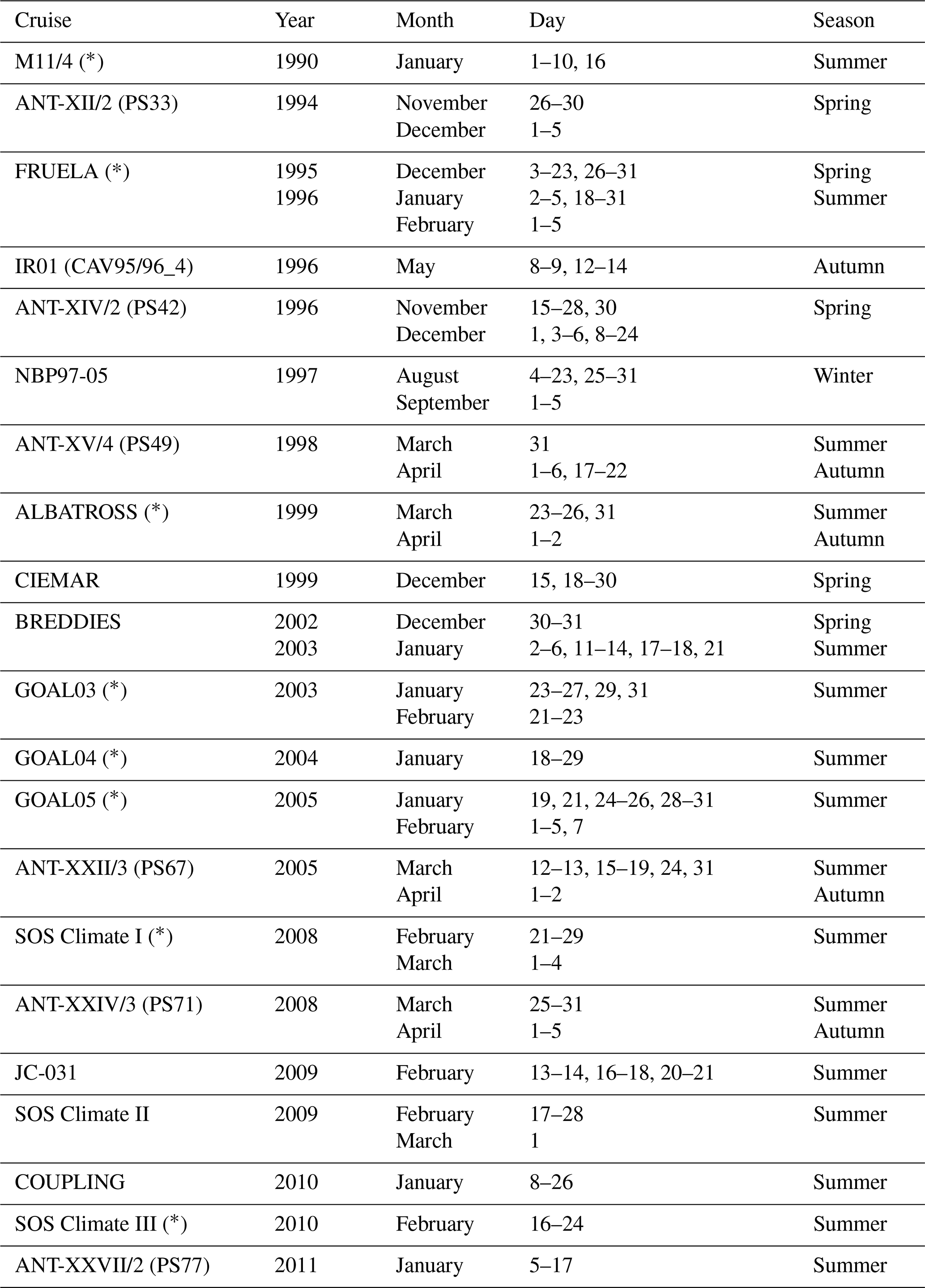
Table A2 Number of profiles available for each cruise and depth used to analyse the goodness of available open-access remotely sensed products of sea surface temperature.

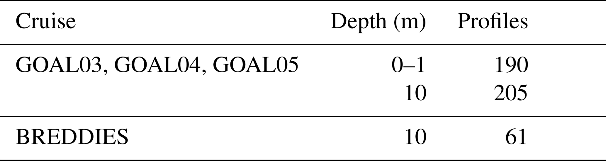
Table A3 R² coefficients for each SST satellite product (OI SST, ESA CCI, OSTIA) compared to in situ SST data from four cruises' data at 0–1 and 10 m depths (see number of profiles in Table A2). The analysis is performed for different study regions: the entire study region (BS and GS) and the Bransfield Strait (BS) surroundings (excluding the GS region).

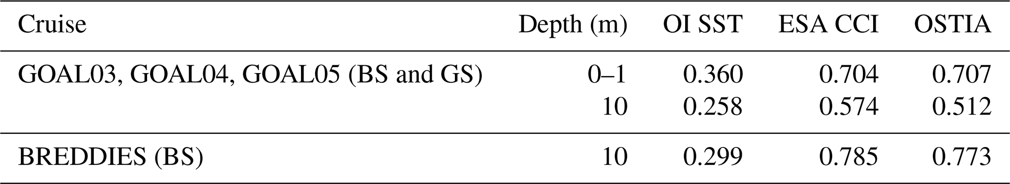
Table A4 The same as Table A2 but here extended to eight cruises for depths of 0–1 m and 21 cruises for depths of 10 m. Regarding the Gerlache Strait region, there are only 5 cruises available for depths of 0–1 m (ALBATROSS, FRUELA, GOAL04, GOAL05, M11/4) and 10 cruises for depths of 10 m (ALBATROSS, FRUELA, GOAL03, GOAL04, GOAL05, M11/4, IR01 (CAV95/96_4), ANT_XXVII/2 (PS77), CIEMAR, JC-031).

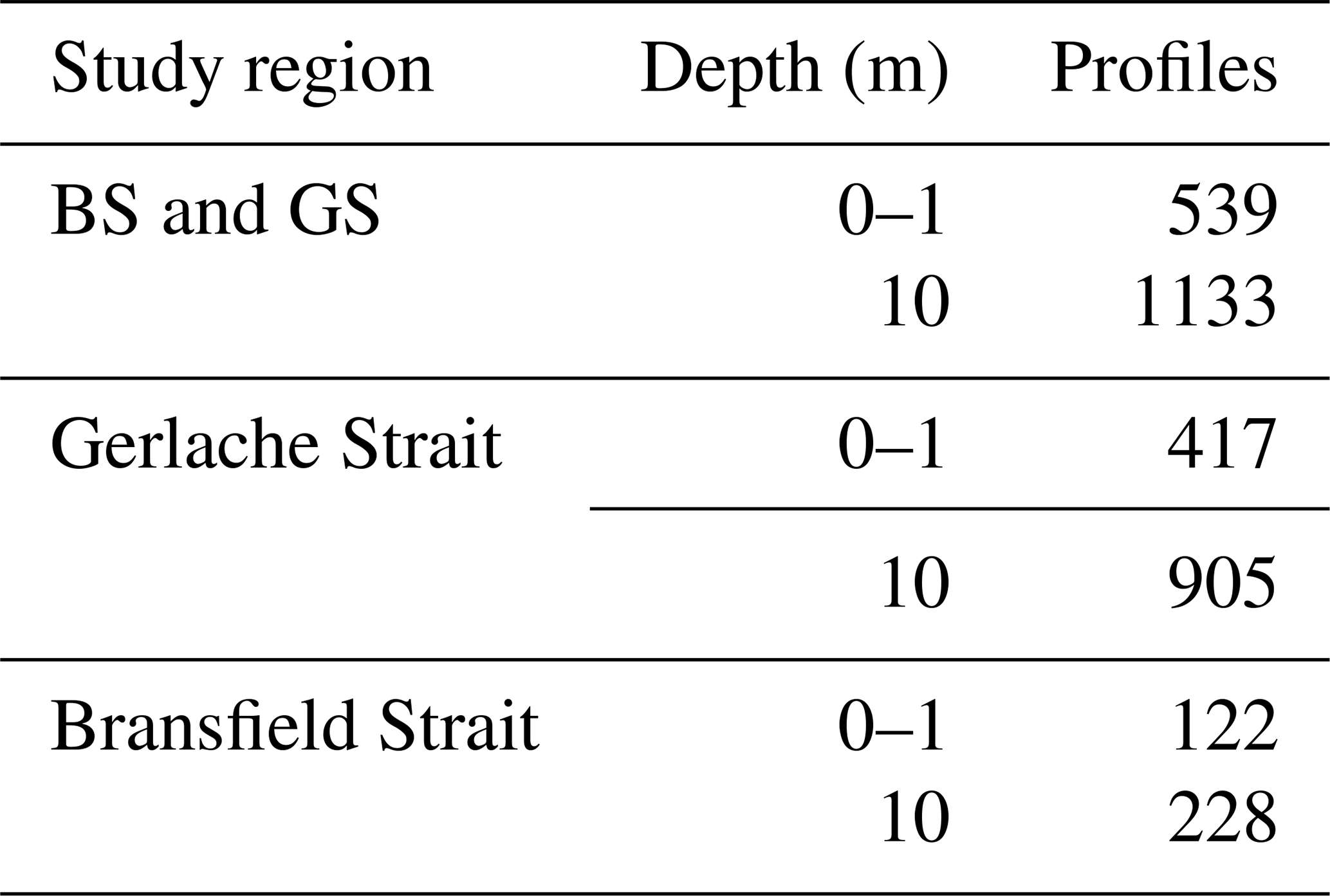
Table A5 R² coefficients for each SST satellite product (ESA CCI, OSTIA) compared to in situ SST data from eight cruises' data at depths of 0–1 m and 21 cruises' data at depths of 10 m (see number of profiles in Table A4). The analysis is performed for different study regions: the entire study region (BS and GS), only the Gerlache Strait (GS) and the Bransfield Strait (BS) surroundings (excluding the GS region).

Appendix B: Frontal probability of the Peninsula Front

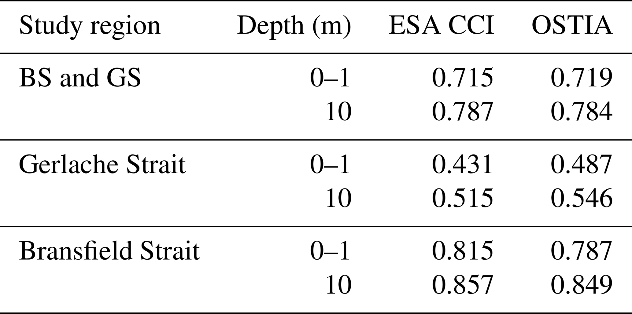
Figure B1 presents the frontal probability (FP; Yang et al., 2023) from the SST and chl-a fields in the Bransfield Strait for the period 1998–2018. The Canny edge-detection algorithm (Canny, 1986) is applied to identify coherent frontal segments. Then, the summertime FP is calculated based on three different cases, using fronts detected on daily data, monthly averaged data and seasonally averaged data over a period of 21 years (in all cases the information corresponds solely to summertime). The FP is defined at each pixel as the times that the pixel is identified as a front as a percentage of the number of total valid pixels for a given time interval.

Results support the choice of the characteristic isotherms and isoline of chl a used in this study to distinguish two different pools of chl-a development in the BS. Additionally, we note that the signal of the Peninsula Front increases in the FP, especially in SST, when based on time-averaged fields (panels b, c, e, f) as compared to daily fields (a, d). We attribute this to the recurrence of the Peninsula Front, which is better defined when a time-averaging procedure is followed before applying the Canny edge-detection algorithm. Simultaneously, a noisier signal emerges regarding other non-recurrent fronts which are present only occasionally in time-averaged fields, thus leading to their presence only in a few fields when computing the FP.

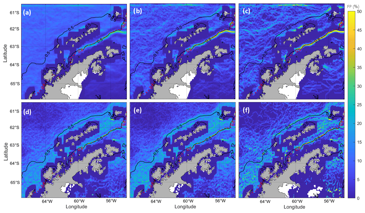
Figure B1 From left to right, the upper panels (a, b, c) show the frontal probability (FP) based on daily, monthly averaged and seasonally averaged data for sea surface temperature across 21 years of summertime. Lower panels (d, e, f) show the same as upper panels but based on chlorophyll-a (chl-a) concentrations. The climatological summertime isotherm of 0.6 °C (dashed red line) and the isoline of 0.5 mg m⁻³ chl-a concentrations (solid black line) as obtained for Figs. 5 and 7 highlight the goodness of our methodology to select them as characteristic environmental values contouring the Peninsula Front in the Bransfield Strait.

We suggest that the FP may be used in future studies to code an automated algorithm capable of monitoring the chl-a blooms in the Bransfield Strait based on remotely sensed SST and chl-a data, using the South Shetland Islands and the Antarctic Peninsula as physical boundaries and the Peninsula Front location as the oceanographic frontier contouring the TBW and TWW pools. Thus, interannually co-locating the alignment of the thermal front and the chl-a spatial distribution will enable the computation of accurate areas of integration for the assessment of the surface blooms acting in the Bransfield Strait.