the Creative Commons Attribution 4.0 License.
the Creative Commons Attribution 4.0 License.
 | 18 Mar 2024
Effects of sea level rise and tidal flat growth on tidal dynamics and geometry of the Elbe estuary
Rita Seiffert
Jessica Kelln
Peter Fröhle
Future global mean sea level rise (SLR) will affect coastlines and estuaries in the North Sea and therefore also coastal protection structures, unique local ecosystems and important waterways. SLR will not only raise water levels but also influence tidal dynamics and morphodynamics, which is why the tidal flats of the Wadden Sea can grow to a certain extent with SLR. Investigations on the effects of climate-change-induced SLR and the related potential bathymetric changes inside of estuaries form an important basis for identifying vulnerabilities and developing appropriate adaptation strategies. To analyse the influence of potential SLR and tidal flat elevation scenarios on the tidal dynamics in the Elbe estuary, we used a highly resolved hydrodynamic numerical model of the German Bight. The analysis results show increasing tidal range in the Elbe estuary solely due to SLR. They also reveal strongly varying changes with different tidal flat growth scenarios: while tidal flat elevation up to the mouth of the estuary can cause tidal range to decrease relative to SLR alone, tidal flat elevation in the entire estuary can lead to an increase in tidal range relative to SLR alone. Further analyses show how the geometric parameters of the Elbe estuary are changing due to SLR and tidal flat elevation. We discuss how these changes in estuarine geometry can provide an explanation for the changes in tidal range.
- Article
(8234 KB) - Full-text XML
- BibTeX
- EndNote


Future global mean sea level rise (SLR), as it is projected for this century (Fox-Kemper et al., 2021), will not only raise water levels in the German Bight but also affect, for example, tidal dynamics (e.g. tidal amplitude and tidal asymmetry) in several ways (Jordan et al., 2021; Wachler et al., 2020). In particular, low-lying coastal areas such as the German Bight and the adjacent estuaries are vulnerable to changes due to SLR. Located in the North Sea, the German Bight includes a large part of the Wadden Sea World Natural Heritage Site. The Wadden Sea is a geologically and ecologically unique region, which is structured into several tidal basins with barrier islands, tidal channels and intertidal areas (Kloepper et al., 2017). As a result of tidal flat morphodynamics (Friedrichs, 2011), SLR will influence not only the tidal dynamics but also the bathymetry in the German Bight. Changes in tidal dynamics affect net sediment transport and therefore bathymetry, which in turn influences tidal dynamics. As the hydrodynamic forces and the coastal profile are interdependent, they strive for a morphodynamic equilibrium in theory (Friedrichs, 2011). Investigations show that in the recent past (1998–2016) most intertidal flats in the German Bight have been vertically growing at higher rates than the observed mean SLR (Benninghoff and Winter, 2019). However, in view of the future acceleration of SLR (Fox-Kemper et al., 2021), it is difficult to quantify to what extent tidal flat growth can keep pace with SLR, and it is questionable whether the present equilibrium between hydrodynamics and morphodynamics will be maintained in the future. Several studies found that tidal flats can potentially grow with SLR if sediment availability is sufficient but cannot keep pace with future high SLR scenarios (Becherer et al., 2018; van der Wegen, 2013; Dissanayake et al., 2012). A precise prediction of the future morphologic development of the Wadden Sea is difficult as it depends not only on the rate of SLR but also on several other factors (e.g. vertical sediment structure, sediment availability and potentially changing meteorology). Furthermore, long-term numerical simulations of morphodynamic processes are challenging, because complex small-scale processes need to be parameterised, and the spatial resolution of morphodynamic simulations is limited by computing power.
Potential tidal flat growth should be considered when studying SLR scenarios, as it strongly affects the tidal dynamics in the Wadden Sea (Wachler et al., 2020; Jordan et al., 2021). SLR in the German Bight will cause an increase in tidal prism relative to channel cross-sectional flow area in the tidal basins, and current velocity in the channels will increase as a result. This effect is counteracted by tidal flat elevation (Wachler et al., 2020). SLR can also cause a shift of the amphidromic point in the German Bight in eastward direction, which is counteracted by tidal flat elevation as well (Jordan et al., 2021). As a result of the changes in amphidromes and current velocities, the combined effect of tidal flat elevation and SLR causes an increase in M2 amplitude in the German Bight relative to SLR alone (Jordan et al., 2021).
One of the main estuaries in the German Bight is the Elbe estuary (Fig. 1), which contains the port of Hamburg and is therefore an important shipping route. The Elbe estuary is the part of the Elbe river that extends from the weir in Geesthacht to the North Sea (Fig. 5). The weir in Geesthacht is the artificial tidal barrier of the estuary. An artificially deepened fairway is maintained from the port of Hamburg to the North Sea to enable the passage of large container ships. The Elbe estuary is a system that is subject to strong anthropogenic influence (e.g. dikes and fairway deepening). While the tidal range in Cuxhaven in the mouth of the estuary remained relatively constant at around 3 m over the last 100 years, the tidal range in St Pauli close to the port of Hamburg increased (Boehlich and Strotmann, 2019). Nowadays, the Elbe estuary is an amplified estuary where the tidal amplitude increases in the upstream direction and reaches its maximum close to the port of Hamburg. Further upstream, where the water depth decreases and river discharge becomes more relevant, the tide is damped and tidal amplitude decreases. The future of the Elbe estuary depends not only on anthropogenic measures implemented on site but also, in particular, on SLR and its implications. SLR and (resulting) topographic changes will alter estuarine geometry and thus influence the tidal wave propagating into the estuary, which is generally modified by amplification, damping, reflection and distortion. The term “estuarine geometry” denotes the form of the intersection of estuarine bathymetry with characteristic local parameters of the tide. SLR will not only simply raise water levels in estuaries; it can also cause changes in water level variations.
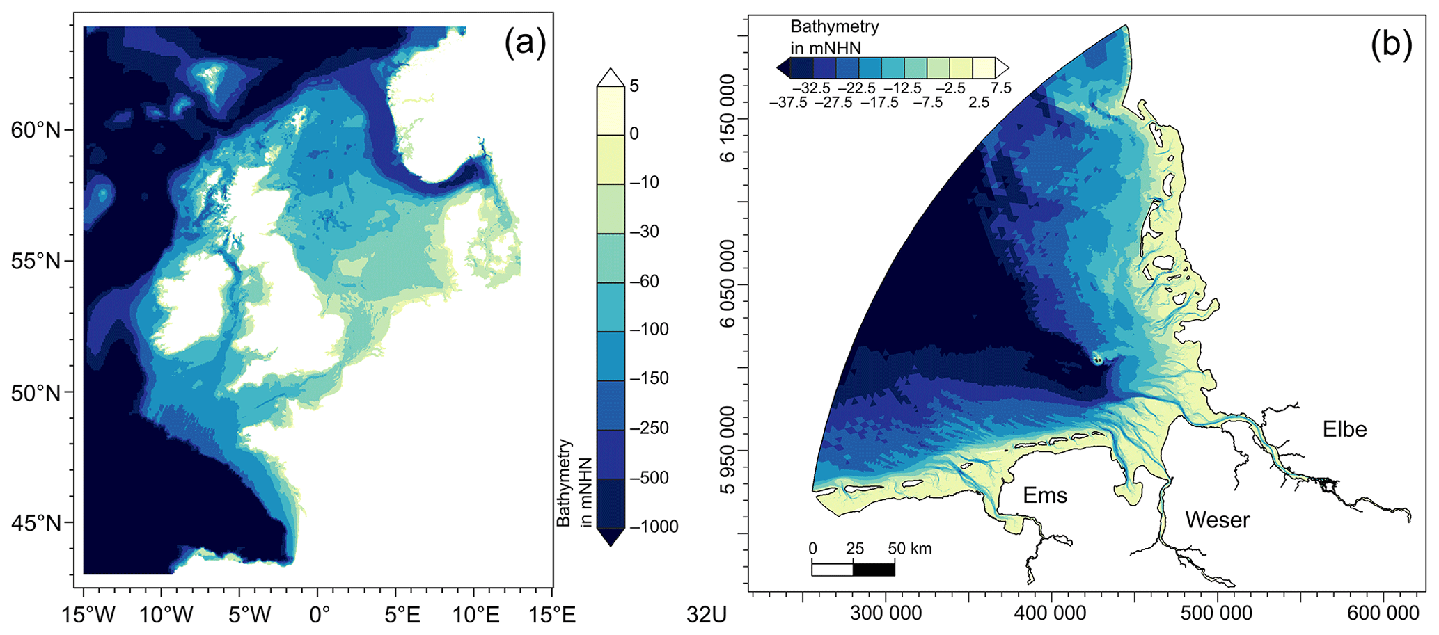
Figure 1Model domain and bathymetry in mNHN (metres Normalhöhennull, German vertical datum) of the DCSMv6FM model (a) in WGS 84 and of the German Bight model (b) in UTM zone 32N.
Higher water levels can help deep-draught vessels navigate the estuary fairway but at the same time can hinder the passage of ships beneath bridges due to reduced clearance. Changes in low tide levels can lead to difficulties in drainage into the estuary and can therefore impact agriculture in the hinterland, navigation in connected channels and tributaries, and urban drainage systems (Khojasteh et al., 2021). Moreover, changes in water level and variations of water levels (low tide and high tide levels) are relevant for the dimensioning of waterfront structures and other hydraulic structures in estuaries (HTG, 2020). In addition, changes in water level and tidal range can affect the inundation time of the intertidal area and can change the location and extension of the intertidal area. This in turn can impact biodiversity and agriculture. Other possible SLR-induced changes in tidal dynamics, besides an increase or decrease in tidal range, are changes in current velocities and tidal asymmetry (e.g. enhanced flood dominance), which can result in more sediment import. A larger tidal range and stronger tidal asymmetry can cause fine sediments to be pumped into the estuary, which can reduce hydraulic drag. This can in turn lead to an increase in tidal amplification eventually resulting in a hyper-turbid state (Winterwerp and Wang, 2013). Such developments in sediment dynamics can impact biodiversity and create economic challenges as a result of the siltation of navigation channels. Another possible consequence of SLR is increased saltwater intrusion into estuaries because of larger tidal prisms and water depths, with an effect on, for example, ecosystems, aquifers and agriculture (Khojasteh et al., 2021). Understanding the future evolution of tidal dynamics due to SLR in heavily utilised estuaries such as the Elbe estuary is therefore important for the development of adaptation measures, e.g. for navigation, port infrastructure and sediment management in the estuary, as well as water management in the hinterland.
Several model-based methods are available to address these questions. Analytical studies have examined the behaviour of tides in estuaries for many decades (Winterwerp and Wang, 2013). Several studies (e.g. Jay, 1991; Friedrichs and Aubrey, 1994; Savenije et al., 2008; Friedrichs, 2010; van Rijn, 2011) developed, discussed and applied analytical solutions to estimate tidal wave propagation in estuaries by simplifying estuarine geometry and the basic equations. They developed scaling parameters to describe the systems while still including the important effects of intertidal area and channel convergence. In these analytical studies, simplified geometric properties of the studied estuaries are considered by the use of several characteristic parameters. However, accurate computation of time-dependent water levels and current velocities requires the application of advanced numerical models that are capable of considering various driving forces and their interactions with accurate concepts of energy exchange and a precise implementation of estuarine shape (Khojasteh et al., 2021). The importance of an accurate representation of the bathymetry of shallow coastal systems in numerical models is pointed out by Holleman and Stacey (2014) and Rasquin et al. (2020). Rasquin et al. (2020) found that insufficient bathymetric resolution may lead to overestimation of the tidal amplitude increase in the German Bight. A study by Seiffert and Hesser (2014) investigating the effect of SLR on the tidal dynamics in the Elbe estuary shows that SLR causes the tidal range in the Elbe estuary to increase. However, this study does not consider the potential vertical growth of tidal flats with SLR. Even if the future morphologic development of the tidal flats in the German Bight and the Elbe estuary is difficult to predict, potential topographic changes might have a considerable impact on tidal dynamics and should not be neglected. A drawback of advanced numerical models, besides the computational time and resources required, is the loss of simplicity and hence transparency. Therefore, extensive analysis of the simulation results is necessary to gain system understanding and provide an insight into how certain parameters affect others. For this purpose, it can be useful to analyse simplified geometric parameters, which were originally developed in the context of analytical estuary models.
In this study, potential future SLR and tidal flat growth scenarios are simulated using a hydrodynamic numerical model. The two issues we want to address in this study are the following. (1) What is the influence of potential future SLR and tidal flat growth scenarios on the tidal range along the Elbe estuary? (2) How can these changes be explained by changes in estuarine geometry? The general aim of this study is to gain a better understanding of the possible effects of potential SLR and tidal flat growth scenarios in the Elbe estuary.
Tidal range is twice the tidal amplitude and the difference between tidal high water and tidal low water. It is an integral part of the energy flux of a propagating tidal wave. As mentioned before, it is a parameter that has an influence on navigation in the estuary and drainage into the estuary, as well as on the dimensioning of bank structures. Moreover, the tidal range in an estuary is closely linked with tidal current velocity, mixing, circulation, sediment transport, water quality and ecosystem communities (Khojasteh et al., 2021). We therefore focus on this parameter, as it is a highly reliable result of hydrodynamic numerical simulations compared to other parameters mentioned. To find explanatory approaches for the changes in tidal range simulated by our hydrodynamic numerical model, we analyse three parameters of estuarine geometry: mean hydraulic depth, convergence of cross-sectional flow area and relative intertidal area. These geometric parameters, which describe the shape of the estuary in a simplified way, are (equally or in similar form) known from previously mentioned analytical models.
The subsequent Sect. 2 describes the applied methods. It includes a short description of the model and the simulated scenarios. The analysed geometric parameters of the estuary and their potential influence on tidal range are shortly discussed in that section. In Sect. 3, the results of the analysed tidal and geometric parameters for some of the examined scenarios are illustrated and outlined. The possible reasons for the detected changes in estuarine geometry and the potential role of a changing geometry in the alteration of tidal range in the estuary are discussed in Sect. 4. Finally, Sect. 5 summarises the main findings of this study and their relevance and suggests questions that should be investigated in future studies.
2.1 Model setup
For this study, the three-dimensional hydrodynamic numerical model UnTRIM2 (Casulli, 2008) is used, which solves the three-dimensional shallow-water equations and the three-dimensional transport equation for salt, suspended sediment and heat on an orthogonal unstructured grid (Casulli and Walters, 2000). A special feature of UnTRIM2 compared to its predecessor, UnTRIM, is the subgrid technology, which allows a high resolution of the topography independently of the computational grid (Casulli, 2008). The computational grid cells can be wet, partially wet or dry, allowing for a precise mass balance and realistic wetting and drying (Sehili et al., 2014), which is important for a realistic representation of the large intertidal areas in the German Bight. The variation of the surface drag coefficient with wind speed is parameterised according to Smith and Banke (1975). The generation of wind waves as well as sediment and heat transport are not calculated in the model setup used for this study in order to reduce computational effort.
The regional model we use is very similar to the model used by Rasquin et al. (2020). The model domain covers the German Bight from Terschelling in the Netherlands to Hvide Sande in Denmark including the estuaries of the Elbe, Weser and Ems rivers with their main tributaries (Fig. 1). The model boundary is defined by the dike line and thus cannot be overflowed. The resolution of the computational grid ranges from 5 km at the open boundary to about 100 m in the coastal area and the estuaries. In the Wadden Sea region and the estuaries, a higher subgrid resolution of about 10 to 50 m in the finest part is used. The model has vertically fixed layers with a resolution of 1 m up to a depth of 27.5 m and a resolution of 10 m below this depth. The topography data of the year 2010 implemented into the model were generated in the EasyGSH-DB project (Sievers et al., 2020).
The atmospheric forcing over the model domain (wind field at 10 m height and surface pressure) is derived from COSMO-REA6 (Bollmeyer et al., 2015). The data are generated and made available by the Hans Ertel Centre of the University of Bonn in cooperation with Germany's National Meteorological Service (Deutscher Wetterdienst, DWD) (Bollmeyer et al., 2015). Salinity is set to a constant value of 33 psu at the open boundary (based on Klein et al., 2016) and 0.4 psu (based on Michael Bergemann, personal communication, 2009) at the upstream boundary of the Elbe estuary.
The German Bight model is used to simulate a spring–neap cycle in July 2013 with a constant river discharge at the upstream boundary of the Elbe estuary of 600 m3 s−1. The weir in Geesthacht is open in the model during the simulated period. The selected period and discharge are chosen to estimate changes in average conditions without extreme events.
Water levels at the seaward open boundary of the German Bight model are provided by the Dutch Continental Shelf Model (DCSMv6FM) (Zijl, 2014), a 2-D hydrodynamic model which covers the northwestern European shelf and which is a further development of DCSMv6 (Zijl et al., 2013, 2015) (Fig. 1). DCSMv6FM uses the flexible mesh technique D-Flow FM (D-Flow Flexible Mesh) (Kernkamp et al., 2011) based on the classical unstructured grid concept. At the seaward open boundary, the DCSMv6FM model is forced by the amplitudes and phases of the 22 main diurnal and semidiurnal constituents, which are derived by interpolation from the data set generated by the GOT00.2 global ocean tide model (Ray, 1999). Sixteen additional partial tides are adopted from FES2012 (Carrère et al., 2013). As for the smaller regional model, the atmospheric forcing for DCSMv6FM is derived from COSMO-REA6 (Hans Ertel Centre for Weather Research; Bollmeyer et al., 2015).
SLR is added at the open boundary of the German Bight model; therefore, SLR-induced changes in tidal dynamics seaward of the German Bight are neglected. Ideally, SLR would be added at the boundary of the shelf model to consider changes in tidal dynamics in the continental shelf seaward of the German Bight model boundary. However, this approach is not suitable in our case, since the resolution of DCSMv6FM is insufficient for estimating SLR-induced changes (Rasquin et al., 2020).
Since the focus of our study is on the Elbe estuary, a brief validation of the model for this specific region is presented below. Further analysis of the model's performance can be found in Rasquin et al. (2020). To compare the simulation results with observations, we simulated seven spring–neap cycles between January and April 2013 with measured river discharge provided by the Federal Waterways and Shipping Agency (WSV, 2022). A comparison of water levels between model results and observations at 39 gauges in the model domain for this period reveals a mean RMSE of 16.4 cm, a mean bias of 7.3 cm and a mean skill score after Willmott et al. (1985) of 0.993. Figure 2 shows a visual comparison between the simulation result and the observation of the water level at the stations of Cuxhaven (mouth of the estuary) and St Pauli (close to the port of Hamburg) for a short period of time. It can be seen that the phase and shape of the vertical tide are well reproduced by the model, but tidal low water is slightly higher in the simulation results compared to the observations. A similar display for an entire spring–neap cycle is shown in Fig. A2 Appendix A. It shows that there are no distinctive differences in performance during the different phases of the illustrated spring–neap cycle.
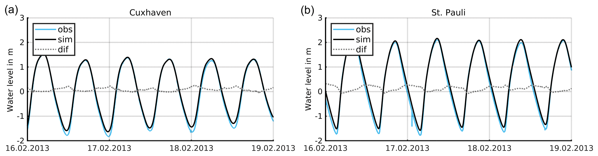
Figure 2Simulated (black) and observed (blue) water levels and the difference between simulation and observation (grey) at the stations in Cuxhaven (a) and St Pauli (b).
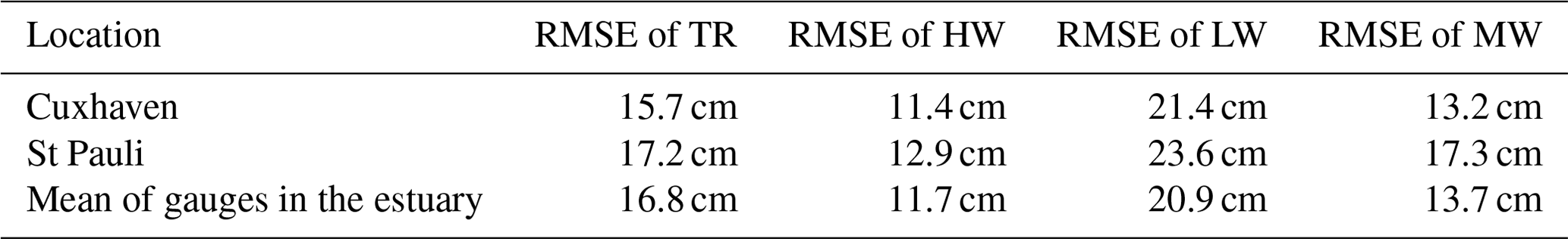
Figure 3 shows the mean tidal range (TR) and mean tidal mean water level (MW) along the estuary for the seven spring–neap cycles, calculated for both the simulation results and observational data at stations along the estuary (WSV, 2022). It demonstrates that the model is able to reproduce the characteristic development of TR along the Elbe estuary, with a strong increase starting at around kilometre 60, a maximum reached around kilometre 115 and a decrease further upstream. As a result of the too high tidal low water, the model underestimates TR by 10–20 cm and overestimates MW by around 10 cm. The RMSE data for the mean TR, MW, tidal high water (HW) and tidal low water (LW) for the gauges Cuxhaven, St Pauli and the mean of 15 gauges in the Elbe estuary are shown in Table 1.
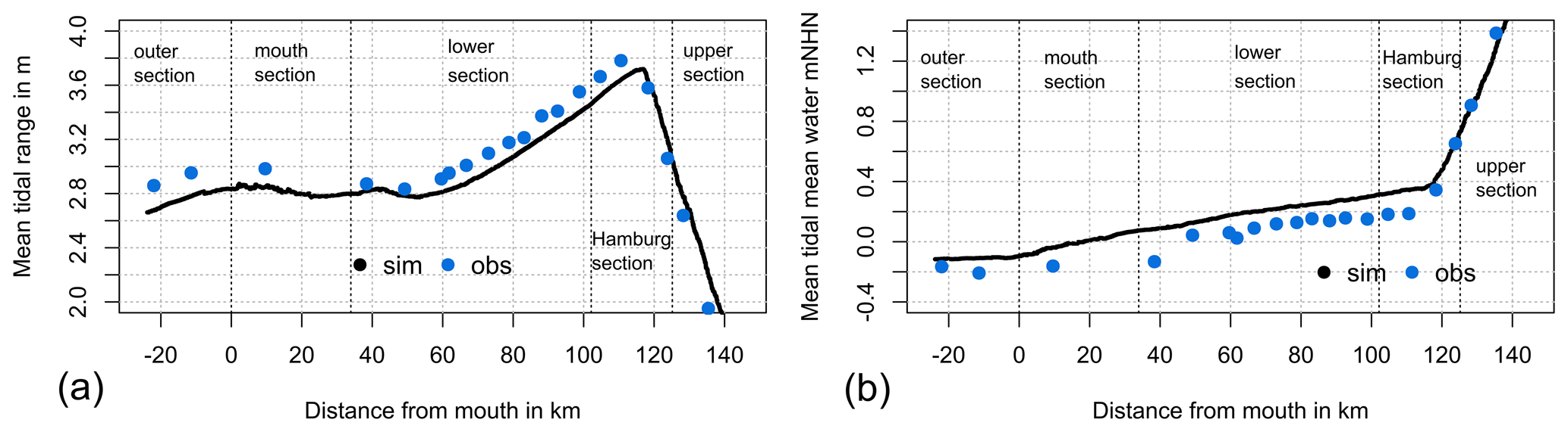
Figure 3TR (a) and MW (b) above mNHN (metres Normalhöhennull, the German datum) averaged over 7 spring–neap cycles from January 2013 to April 2013 along the Elbe estuary, calculated from observations (blue) and from simulation results (black).
Table 1Root-mean-square error for tidal parameters of water level in the Elbe estuary.
2.2 Simulated scenarios
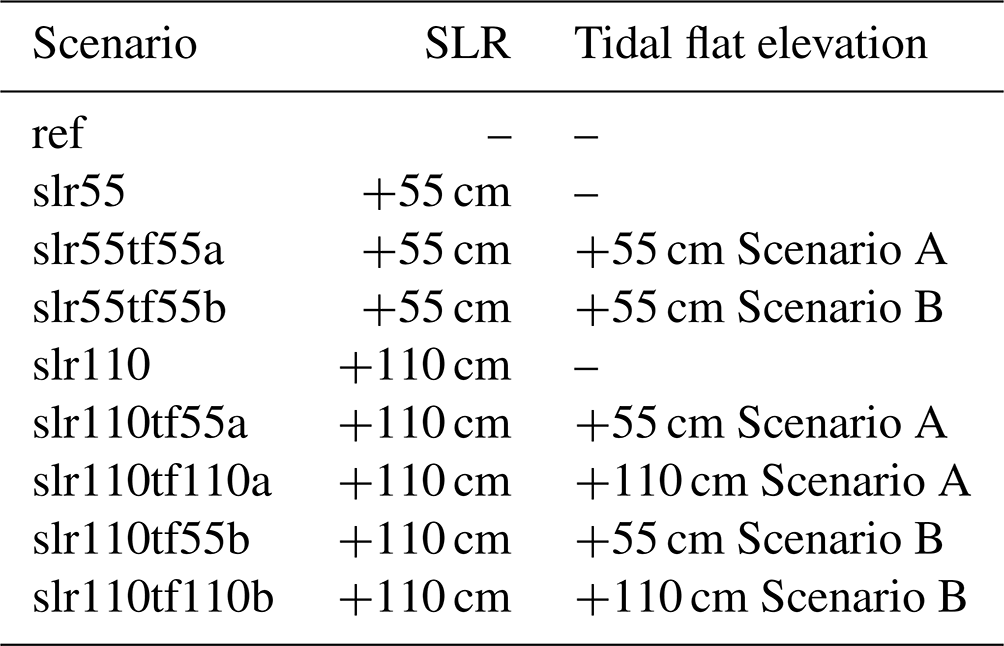
To investigate the effect of SLR and potential corresponding tidal flat growth, several scenarios are simulated and analysed. Two SLR scenarios of 55 and 110 cm were simulated by adding SLR at the open boundary of the German Bight model. According to the IPCC Sixth Assessment Report (AR6), mean global SLR in 2100 compared to the reference period 1995–2014 will be in the likely range between 0.43 and 1.01 m for the intermediate- to high-emission scenarios (SSP2-4.5, SSP3-7.0 and SSP5-8.5) (Fox-Kemper et al., 2021). Our selected SLR scenarios are close to the median of the intermediate scenario and close to the upper range of the high-emission scenario for 2100. Projected values for regional SLR in the southeastern North Sea region (Delfzijl, Cuxhaven, Esbjerg) are within a range of ±20 cm of the median of the projected global mean SLR until 2100 (Fox-Kemper et al., 2021; Garner et al., 2021).
As mentioned in the Introduction, there are uncertainties and difficulties in quantifying to what extent the tidal flats in the German Bight will be able to keep up with future accelerated SLR. The amount of tidal flat accretion can strongly differ between the tidal basins of the German Bight and not only depends on future SLR acceleration and magnitude but also on sediment availability and meteorological conditions. To gain a better understanding of the possible effects of potential SLR and tidal flat growth in the Elbe estuary, we analyse a range of 0 %, 50 % and 100 % tidal flat growth with SLR. In these scenarios, all tidal flat areas in the model domain are uniformly elevated by the same amount, which is a highly simplified assumption.
The scenarios with tidal flat growth are further differentiated firstly by elevating the tidal flats in the German Bight and in the mouth section of the Elbe estuary (Scenario A) and secondly by elevating the tidal flats in the German Bight, the mouth section and also the lower section of the estuary (Scenario B) (see Fig. 4). The purpose of this differentiation inside the estuary is to gain a better understanding of the estuarine system in the context of SLR and tidal flat elevation. Table 2 summarises the scenarios simulated with the German Bight model. The letters “a” and “b” in the names stand for Scenarios A and B, while “tf” stands for “tidal flats”.
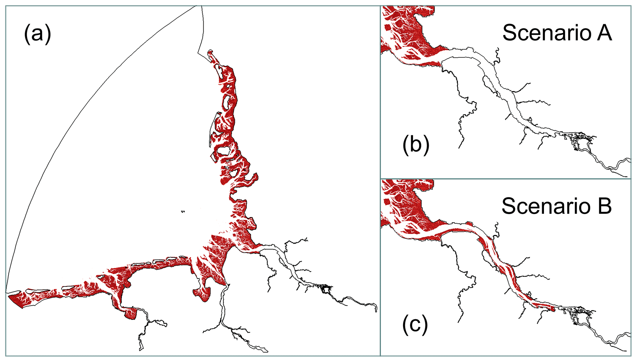
Figure 4Areas of tidal flat elevation in the model domain (a) and in the Elbe estuary for two different scenarios (b) and (c).
2.3 Analysis of simulation results
2.3.1 Spatial decomposition and definition
Our study area is the Elbe estuary, i.e. the tidally influenced part of the river Elbe that extends from the weir in Geesthacht to the North Sea (Fig. 5). The weir in Geesthacht is the artificial tidal barrier of the estuary. The estuary splits into two branches that reunite close to the port of Hamburg (Fig. 5). To enable the passage of large container ships travelling to Hamburg, an artificially deepened fairway is maintained up to the port. The part of the estuary between Hamburg and the city of Brunsbüttel includes intertidal areas and several islands and is connected to a number of small tributaries (Fig. 5). The widening mouth of the estuary with its large intertidal areas interfused by several smaller and larger channels is located between Brunsbüttel and Cuxhaven.
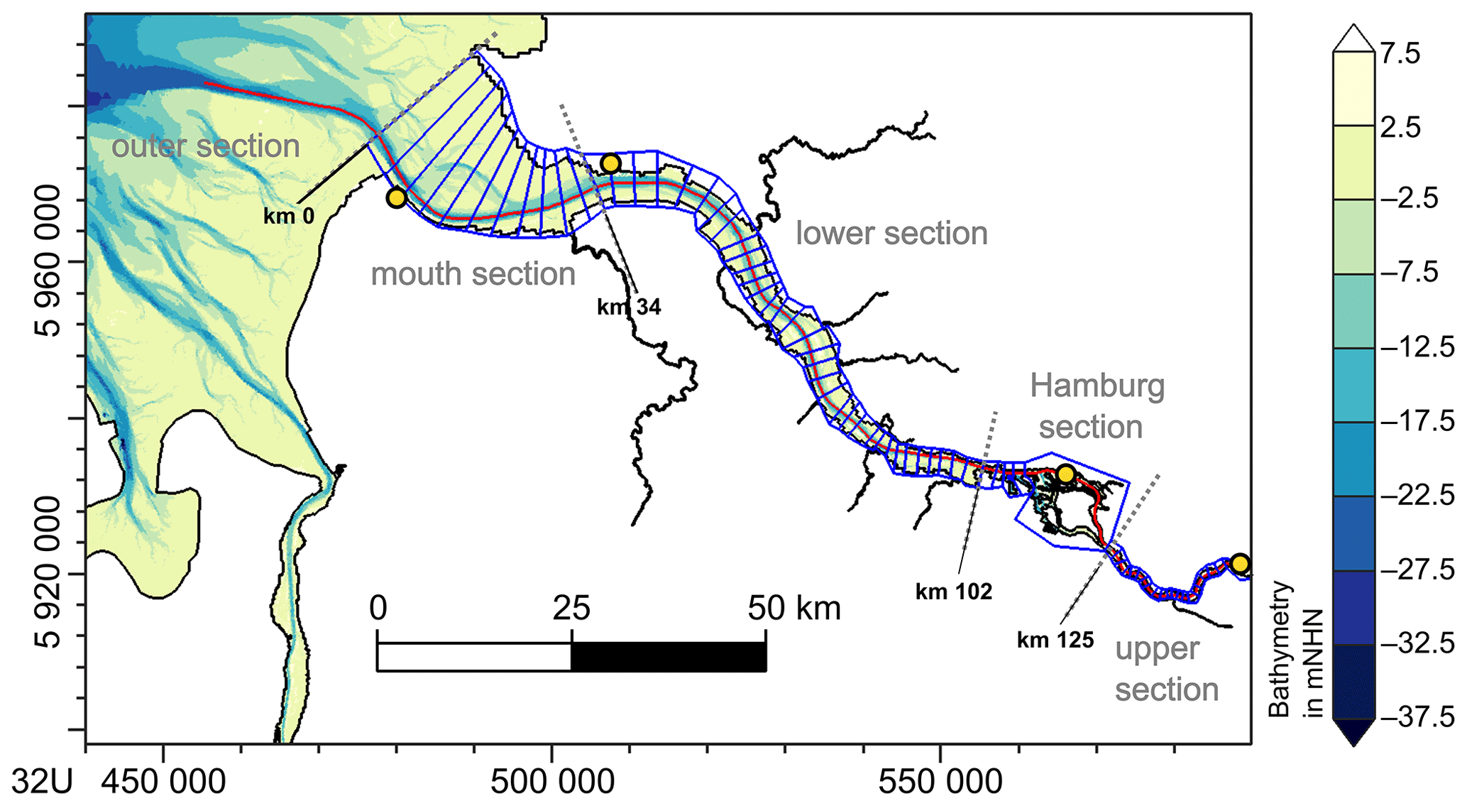
Figure 5Model excerpt of the Elbe estuary showing the profile along the estuary (red) and a subdivision into five sections (grey) and 71 control volumes (blue) that are used for the analysis of the simulation results. The yellow markers represent the following locations from left to right: Cuxhaven, Brunsbüttel, St Pauli (Hamburg Port) and Geesthacht.
Mean tidal parameters are analysed and visualised along the profile of the estuary. The profile is displayed in Fig. 5; it starts seaward of the mouth of the estuary and runs upstream along the fairway and the northern branch up to the weir in Geesthacht. For the analysis of the geometric parameters, the estuary is divided into 71 control volumes (Fig. 5). As the Elbe estuary splits into two branches, which reunite close to the port of Hamburg and enclose the island of Wilhelmsburg, this region is contained in one relatively large control volume compared to the other control volumes. The control volumes and, consequently, the analysed geometric parameters do not cover the full length of the estuary profile, as a clear definition of the boundaries is not possible in the outer section of the estuary. However, the tidal parameters are analysed and displayed along the entire profile, even in the outer section. For a better comparison between the tidal parameters along the profile and the geometric parameters derived for the control volumes, the zero position of the x axis in the figures showing the results along the estuary is set at the most seaward control-volume boundary of the profile. Furthermore, the estuary is roughly divided into five sections, which are shown in Fig. 5 and referred to (from west to east) as outer section, mouth section, lower section, Hamburg section and upper section.
2.3.2 Tidal and geometric parameters
The results of the hydrodynamic numerical simulation are analysed by calculating the characteristic parameters of the vertical tide for the domain of the Elbe estuary. Further details about the method of the applied tidal analysis can be found in Lang (2003) and BAW (2010). All parameters are analysed for one spring–neap cycle in July 2013, simulated with a constant discharge of 600 m3 s−1. The mean tidal parameters of the spring–neap cycle are analysed and visualised along the profile of the estuary shown in Fig. 5. This study mainly focuses on the changes in mean tidal range (TR). TR is a key parameter in the estuary for characterising tidal dynamics, as it is closely linked to other tidal parameters (e.g. low water (LW), high water (HW)) which are relevant for navigation, drainage into the estuary and dimensioning of hydraulic structures. To derive explanatory approaches for the changes in TR, the changes in the estuarine geometry are analysed. The geometric parameters are obtained by analysing the values for the 71 control volumes/areas along the estuary shown in Fig. 5. In the following section, the three geometric parameters studied will be introduced: convergence length (La), mean hydraulic depth (h) and relative intertidal area (ϙSINT). The tidal dynamics in an estuary are influenced by its geometry in several ways. As our focus is on TR, we shortly discuss the potential influence of these three geometric parameters on TR in an estuary.
2.3.3 Convergence length
Background
Upstream convergence of an estuary can cause upstream amplification of tidal waves. This phenomenon is also known as “wave shoaling” or “wave funnelling” (van Rijn, 2011). The tidal wave amplification due to the gradual change in the width and depth of a system can be explained with the wave energy flux equation as described in Green's law 1837 (van Rijn, 2011):
where F is the energy flux per unit time (wave period) of a progressive sinusoidal wave being equal to E the energy of the wave per unit length of the wave times c=(gh)0.5 the wave propagation celerity in shallow water. H is the tidal wave height (tidal range), b is the width of the channel, h is the water depth, ρ is the water density and g is the gravitational acceleration. According to Green's law, when the tidal wave is assumed to be a progressive sinusoidal wave in a system without reflection and energy loss due to friction, energy flux is constant and it follows that tidal amplitude varies as with the channel width (b) of the momentum-conveying stream and the depth (h) below mean tidal water level (Jay, 1991). In an estuary containing a channel and tidal flats, the amplitude varies as , where bT is the width at mean water level (Jay, 1991). Based on these considerations, a gradual upstream decrease in the cross-sectional flow area A (A=hb) can cause an increase in tidal amplitude and therefore TR, and an increase of A can cause a decrease in TR accordingly.
Analysis of convergence length
A funnel-shaped geometry with decreasing width and depth in the upstream direction is typical of most alluvial estuaries (van Rijn, 2011). A schematic plan view of a funnel-shaped estuary is shown in Fig. 6. A mathematical way to represent the shape of an estuary, which has been used in many studies (Gisen, 2015), is an exponential function in the form of
where A is the cross-sectional area, A0 is the cross-sectional area at x=0 (mouth of the estuary), x is the distance from the mouth of the estuary in the upstream direction along the estuary axis and La is defined as convergence length (the distance from the mouth at which the tangent through the point (0, A0) intersects with the x axis) (Savenije, 2012). The parameter La describes the rate of the decrease in the cross-sectional area in the upstream direction. When comparing the convergence length between different estuaries or between different scenarios of the same estuary, a smaller value of La indicates a stronger convergence. It should be noted that some studies use the convergence length based on width (and sometimes depth), instead of the convergence length of cross-sectional area (A) to describe the shape of an estuary. Furthermore, several studies calculate more than one convergence length for an entire estuary by dividing it into sections with distinct convergence lengths. However, we calculate only one convergence length (La) for the entire estuary to analyse possible changes in convergence for the entire system. We analyse La for each simulated scenario by fitting the exponential function of Eq. (2) to the data of the mean cross-sectional flow area at the control-volume boundaries along the estuary, which are derived by analysing the simulation results. The mean cross-sectional flow area is derived by averaging the mean cross-sectional flow area of each tide over the spring–neap cycle. The exponential function is fitted with a weighted multiple nonlinear least-square regression using the Gauss–Newton algorithm. The regression is performed with the package “nlstools” of the R project (Baty et al., 2015). A multiple regression is necessary to analyse whether the convergence lengths of the different scenarios are significantly differing. A weighted regression is conducted to reduce the effect of uneven data distribution along the x axis due to unevenly sized control volumes.
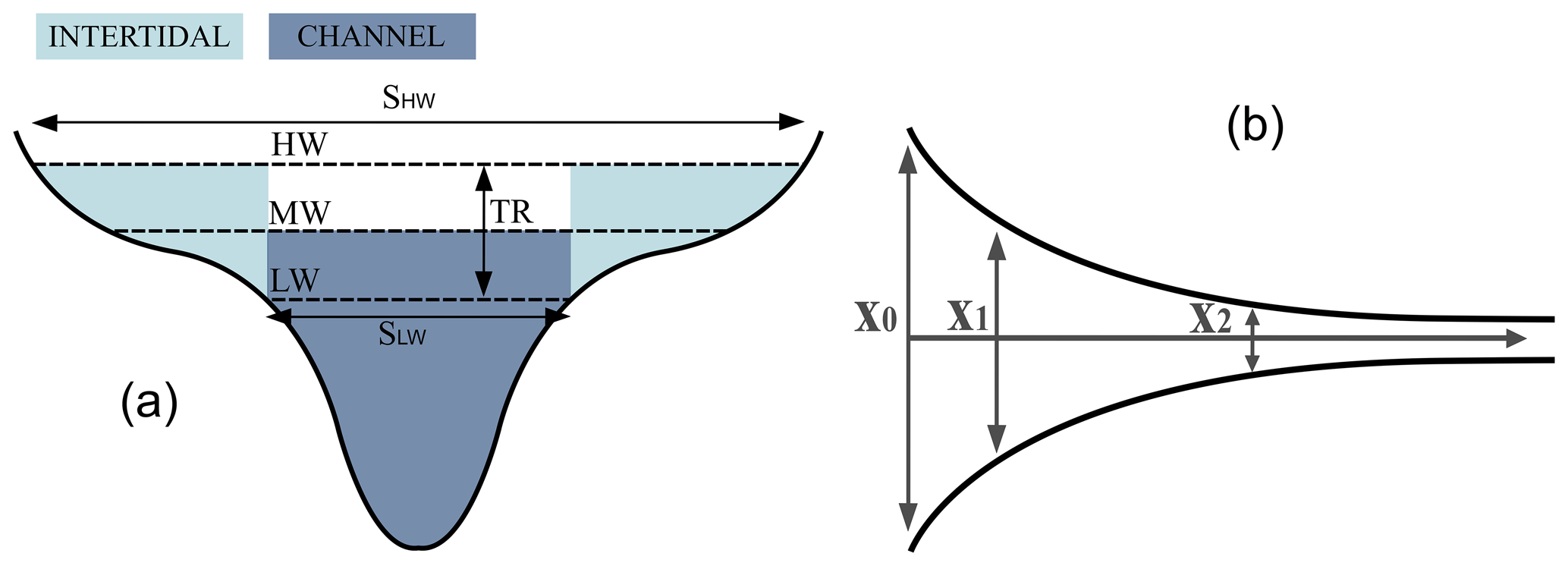
Figure 6(a) Schematic cross-section with channel and intertidal volume, high water (HW), mean water level (MW) and low water (LW), tidal range (TR) and surface area at HW and LW (SHW and SLW); (b) schematic plan view of a funnel-shaped estuary.
2.3.4 Mean hydraulic depth
Background
Water depth influences the propagation speed of a tidal wave c in shallow water in the form of c=(gh)0.5. According to the wave energy flux equation mentioned above (Eq. 1), an increase in water depth can therefore increase wave propagation speed and diminish TR if all other parameters remain constant. However, this would be a simplified assumption as it excludes bottom friction and other shallow water effects which become increasingly important closer to the coast where the ratio of tidal amplitude (a) to water depth (h) increases. Energy dissipation due to work done by bed shear stress causes damping of the wave (decrease in TR). The water depth in an estuary therefore affects the frictional damping of a tidal wave due to energy dissipation which scales by the cube of current velocity over depth () (Simpson and Hunter, 1974; Garrett et al., 1978). Therefore, a greater mean water depth in the estuary can have the effect of increasing TR by reducing frictional damping of the tidal wave and vice versa. Furthermore, a change in mean water depth can also lead to a change in TR by pushing the system closer to or away from resonance (Talke and Jay, 2020).
Analysis of mean hydraulic depth
The depth over an estuary cross-section (Fig. 6) can be highly variable due to deep channels and shallow intertidal areas. The mean hydraulic depth of an estuary can be defined and calculated in several ways (Zhou et al., 2018). Many studies with simplified models assume that the flow-conveying cross-section solely comprises the channel, excluding the intertidal area. Mean hydraulic depth can thus be defined either including or excluding the intertidal area, which has a strong influence on the resulting value. The two different definitions, one including intertidal area in the calculation of mean hydraulic depth (ht) and the other excluding it from the calculation (hc), are
and
where VMW, SMW, VLW and SLW are the volume (V) and the surface area (S) at mean water level (MW) and mean low water level (LW), respectively (see Fig. 6). We calculate the mean hydraulic depth in each control volume and section for each scenario by using the volume and wetted surface area of the control volumes from the simulation results. Mean hydraulic depth is calculated according to Eq. (3) for the entire cross-section (ht) and according to Eq. (4) for the channel part of the cross-section only (hc). The mean volume (V) and wetted surface area (S) at MW and LW are derived by averaging over the spring–neap cycle.
2.3.5 Relative intertidal area
Background
The intertidal area is approximately the area of the tidal flats between tidal low water (LW) and tidal high water (HW), which is subject to wetting and drying cycles. Along-estuary transport of mass and momentum over tidal flats is often assumed to be negligible (Friedrichs, 2010). Tidal flats mainly store water instead of transporting momentum along the estuary (Aubrey and Speer, 1985). Momentum is lost as water flows onto the tidal flats with rising tide and decelerates because of strong friction, and also with falling tide, as water with zero momentum returns to the momentum-carrying channel and must be accelerated (Jay, 1991). Therefore, a loss of intertidal area causes an increase in tidal amplitudes, and an enlargement of intertidal area causes a decrease in tidal amplitude (Jay, 1991). According to Song et al. (2013), tidal flats affect the tidal energy budget by storage and dissipation, while the former can be more significant than the latter. This means that an increase in the relative intertidal area (ϙSINT) can cause a decrease in TR and vice versa.
Analysis of the relative intertidal area
A tidal basin or an estuary can be roughly divided into a subtidal (SLW) and an intertidal area (SINT) (Fig. 6). The intertidal area (SINT) is defined as the difference between wetted surface area at mean high water and wetted surface area at mean low water:
The relative intertidal area (ϙSINT) can be defined as the ratio between SINT and SHW:
Different ratios are commonly used to describe the cross-sectional geometry and can often be converted into each other. They are discussed in detail by Zhou et al. (2018). We define relative intertidal area as the ratio of intertidal area to wet surface area at mean high water (ϙSINT) (Eq. 6). According to Eq. (6), we calculate the relative intertidal area for each control volume and section for each scenario. The mean wetted surface area at HW and LW is derived from the simulation results for each control volume and averaged over the spring–neap cycle.
3.1 Tidal range along the estuary
In Fig. 7, tidal range (TR) is visualised for the different simulated scenarios along the profile of the estuary. Other parameters of the vertical tide (high water (HW), low water (LW), mean water (MW)) can be found in Appendix A (Fig. A1). We focus on the results of the scenarios with 110 cm SLR to gain a better system understanding. The results of the scenarios with SLR of 55 cm are not shown here in detail but are included to determine whether the changes due to SLR are in principle similar for a different SLR scenario. As apparent in Fig. 7, the mean tidal range (TR) in the Elbe estuary increases in the upstream direction to reach a maximum in the Hamburg section and decrease subsequently. The simulation result for the scenario with SLR of 110 cm (slr110) reveals an increased tidal range (TR) due to lower LW and higher HW relative to the applied SLR of 110 cm. TR is increased by up to around 15 cm in the mouth section and by around 10 cm in the lower section. Upstream of the Hamburg section the increase intensifies, mainly due to a lower LW. If tidal flats are elevated by 50 % with SLR in scenario A (slr110tf55a), no notable changes in TR are visible compared to scenario slr110. If, however, tidal flats in the German Bight and the mouth section of the estuary are fully (100 %) elevated with SLR (slr110tf110a), TR is damped relative to scenario slr110. In contrast, an additional elevation of the tidal flats in the entire Elbe estuary (slr110tf110b and slr110tf55b) strongly increases TR relative to scenario slr110, especially in the lower section.
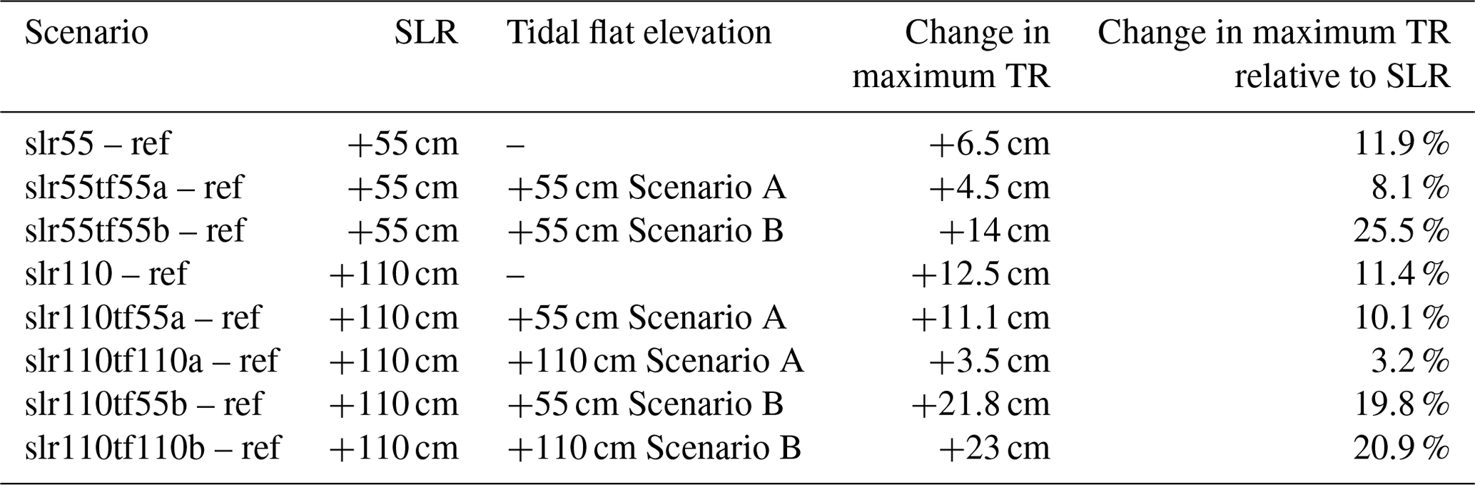
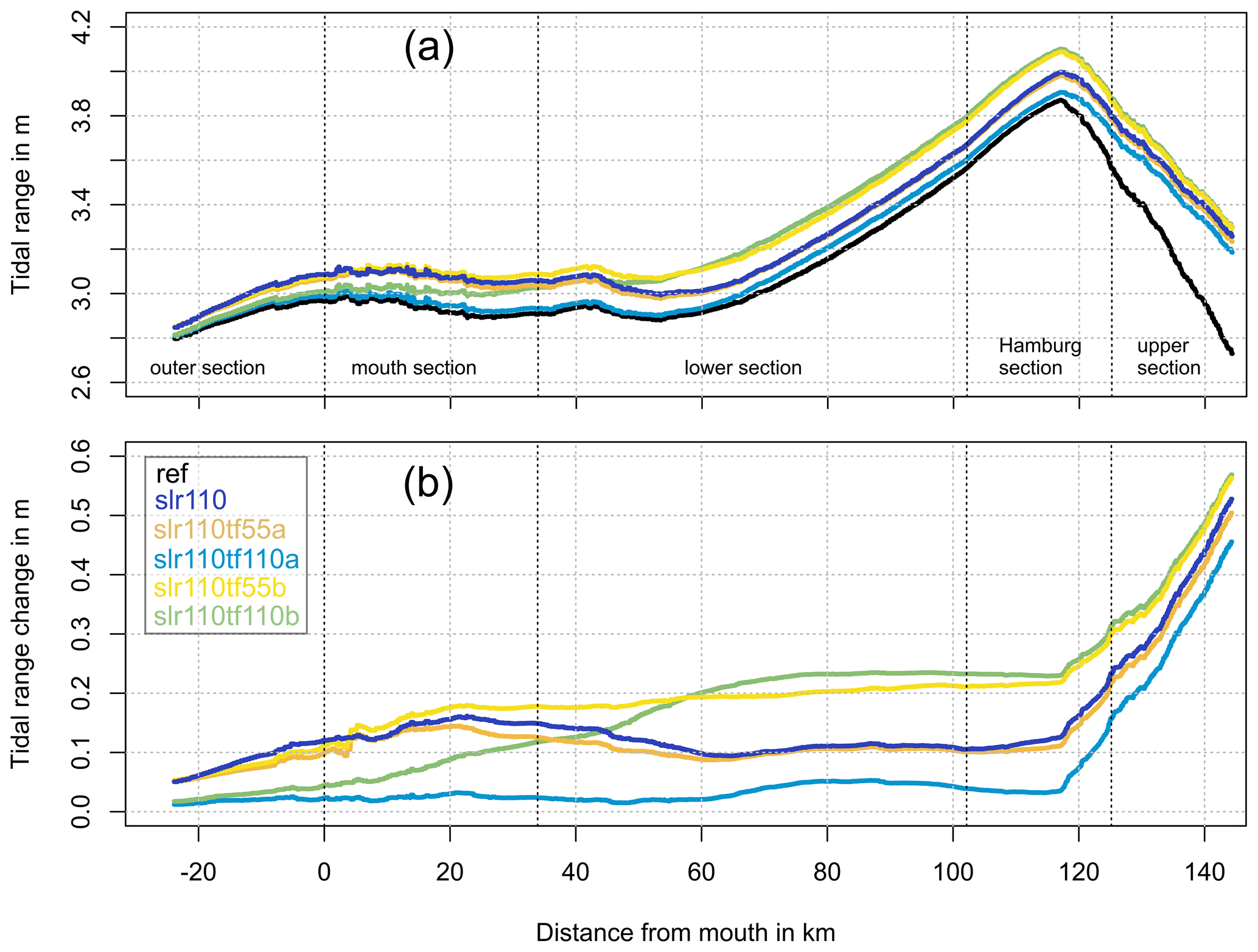
Figure 7TR (in m) (a) and change in TR relative to reference condition (in m) (b) along the estuary profile analysed for a spring–neap cycle for scenarios ref (black), slr110 (dark blue), slr110tf55a (orange), slr110tf110a (light blue), slr110tf55b (yellow) and slr110tf110b (green).
For all scenarios, the maximum value of TR along the estuary is reached in the Hamburg section. Table 3 lists the changes in maximum TR relative to the reference condition (maximum TR=3.87 m) for all simulated scenarios with SLR 110 cm as well as SLR 55 cm. Maximum TR increases by 6.5 cm for a SLR of 55 cm and by 12.5 cm for an SLR of 110 cm, which is about 11 %–12 % of the respective SLR. Both SLR scenarios with 100 % tidal flat elevation in Scenario A (slr55tf55a and slr110tf110a) show an increase in maximum TR that is less than with SLR alone. In both SLR scenarios with 100 % tidal flat elevation in Scenario B (slr55tf55b and slr110tf110b) the increase in maximum TR is greater than in the scenarios without tidal flat elevation.
3.2 Changes in estuarine geometry
3.2.1 Convergence length of cross-sectional flow area
Figure 8 shows the mean cross-sectional flow area (A) at the control-volume boundaries along the estuary. For better readability, the results of the scenarios slr110tf55a and slr110tf55b are not shown. The depicted flow area is the mean area through which the tidal water flux flows, averaged over one spring–neap cycle. The results show a typical upstream decrease in A in all scenarios. As a result of SLR (scenario slr110), A increases along the estuary relative to the reference scenario. Elevated tidal flats in the mouth of the estuary (slr110tf110a and slr110tf55a) cause A to decrease in this section compared to slr110. Additional elevated flats in the lower section of the Elbe estuary (slr110tf110b and slr110tf55b) slightly decrease A in this section accordingly.
Table 4Results of the multiple nonlinear least-square regression for the cross-sectional flow area along the estuary fitted to Eq. (2). Results with a p value>0.1 are considered not significant (n.s.).
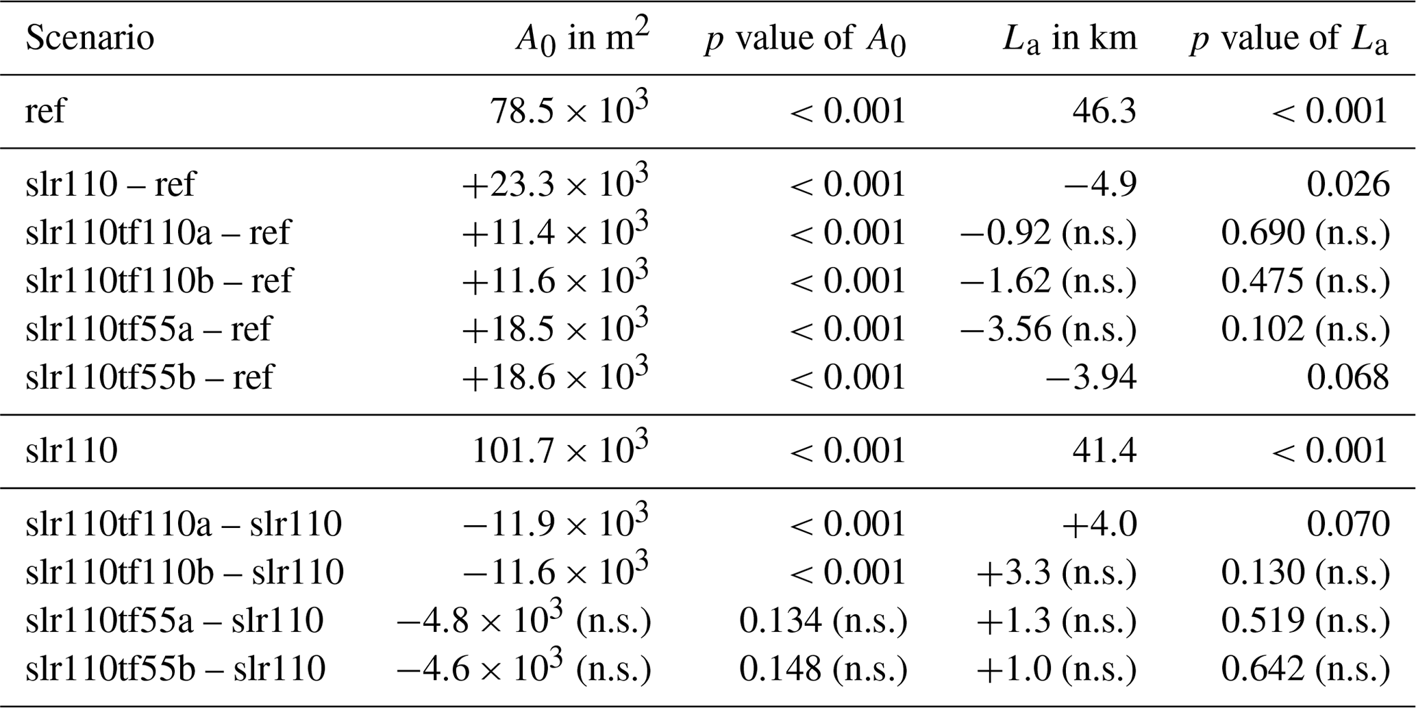
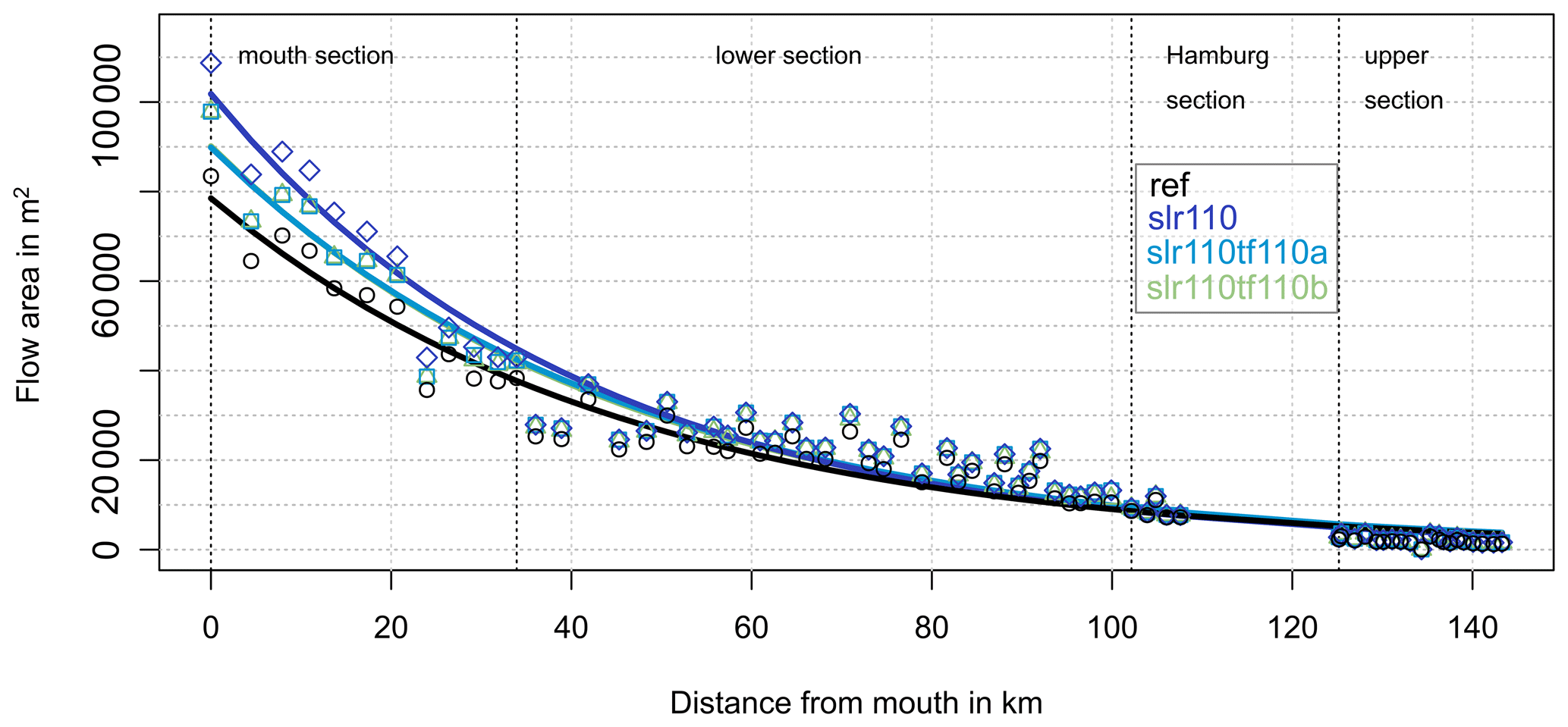
Figure 8Cross-sectional flow area A analysed for each control-volume boundary along the estuary profile (markers) and fitted regression model (lines) for the scenarios ref (black), slr110 (dark blue, rhombuses), slr110tf110a (light blue, squares) and slr110tf110b (green, triangles). (The results of scenarios slr110tf55a and slr110tf55b are not shown in the figure for better readability.)
The geometric parameter of convergence length (La) is calculated by fitting an exponential function (Eq. 2) to the data sets (see Sect. 2.3.3). To determine whether the convergence length significantly changes between two scenarios, a multiple regression is performed. The results of the weighted multiple nonlinear least-square regression for all scenarios compared to the reference condition and to slr110 are shown in Table 4.
The derived convergence length (La) of the Elbe estuary for the mean cross-sectional flow area (A) of the spring–neap cycle is 46.3 km in the reference condition and 41.4 km in the scenario slr110. Depending on the p value for the difference of La between two scenarios, the null hypothesis of no change in convergence length La can or cannot be rejected. We decided to consider a significance level of α=0.1. For the difference between La of the scenarios slr110 and ref (reference), the null hypothesis can be rejected. The detected significant decrease in La indicates a stronger convergence and hence a stronger rate of decrease in A in the upstream direction due to SLR of 110 cm. The results further show that in scenario slr110tf110a convergence is significantly weakened compared to scenario slr110, and not significantly different compared to the reference scenario. For the difference between the scenarios slr110tf55a and ref, we detect a significant decrease in La and hence a stronger convergence. For the scenarios slr110tf55a and slr110tf110b, we cannot detect a significant change in La relative to the reference scenario or to slr110. However, the results for La and their p values (0.102 and 0.13) indicate that La for scenario slr110tf110b is larger than for slr110 and very similar to the reference condition, while La for slr110tf55a is similar to slr110.
3.2.2 Mean hydraulic depth
As mentioned in Sect. 2.3.4, the mean hydraulic depth for each section and for each scenario is calculated in two different ways, i.e. including (ht) and excluding (hc) intertidal area in the calculation of hydraulic depth. The resulting mean hydraulic depth values for the reference condition and each slr110 scenario and section are shown in Table 5. Figure 9 illustrates the relative change in mean hydraulic depth of the scenarios slr110, slr110tf110a and slr110tf110b relative to the reference scenario (ref) for each control volume and section.
The results indicate that SLR of 110 cm (slr110) does not in general cause an increase in mean hydraulic depth along the estuary. As shown in Fig. 9, the relative change in ht and hc is strongly scattered with an increase in some control volumes and a decrease in others. In the mouth section ht increases upstream of kilometre 20 and decreases downstream. Averaged over the sections, slr110 has almost no impact on ht in the mouth section and causes it to decrease slightly in the lower section and increase in the Hamburg section and the upper section. In the scenarios slr110tf110a and slr110tf110b, mean hydraulic depth clearly increases in the regions where the tidal flats are elevated, and scatter is reduced in these regions. The changes in hc are qualitatively similar to ht except that mean hydraulic depth excluding intertidal area (hc) shows a stronger decrease solely due to SLR in the mouth section.
Table 5Mean and standard deviation (SD) of hydraulic depth of the entire cross-section (ht) and of the channel (hc) in the Elbe estuary (in m).
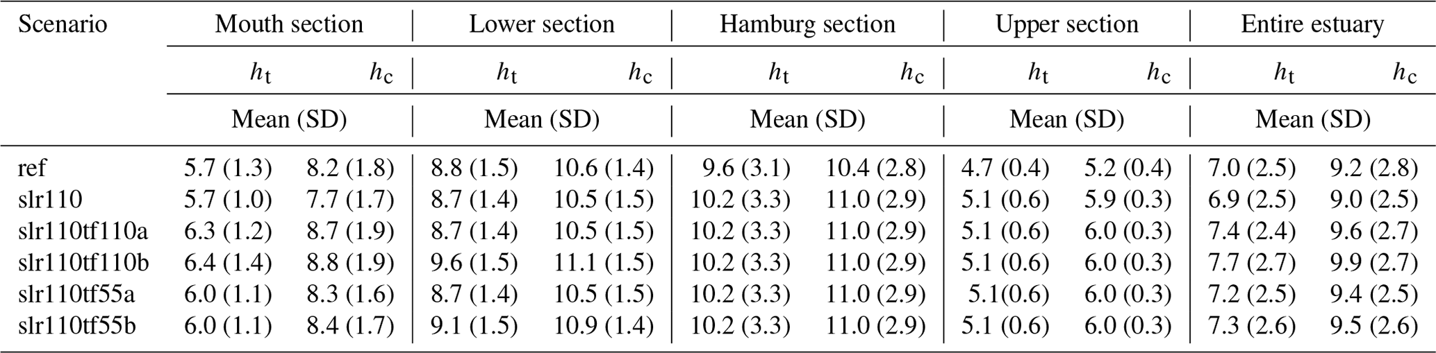
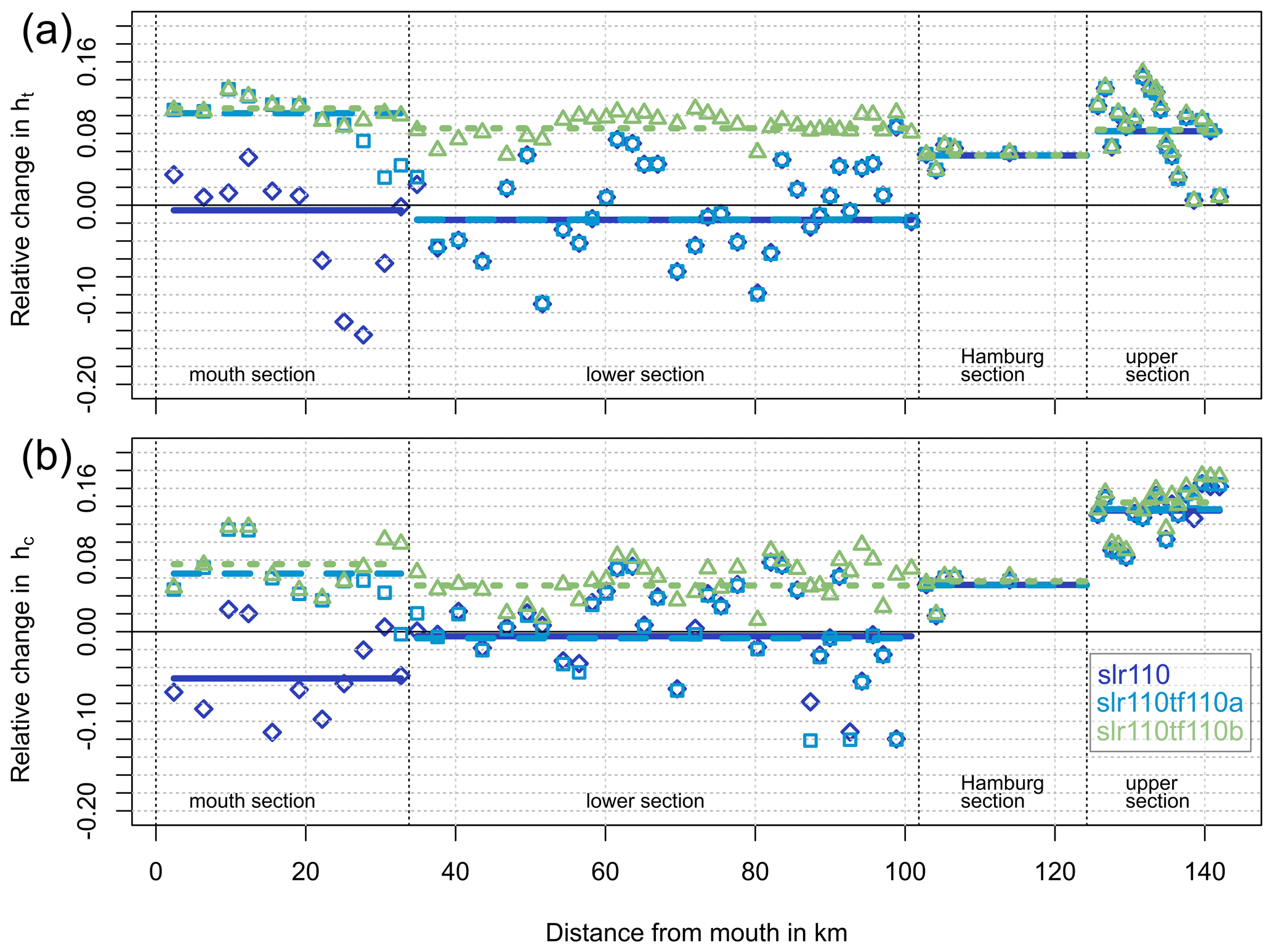
Figure 9Relative change in mean hydraulic depth (a, ht, and b, hc) in each control volume (markers) and each section (lines) relative to reference condition for scenarios slr110 (dark blue rhombuses), slr110tf110a (light blue squares) and slr110tf110b (green triangles). (The results of scenarios slr110tf55a and slr110tf55b are not shown in the figure for better readability.)
3.2.3 Mean relative intertidal area
The mean relative intertidal area (ϙSINT) in each section along the estuary is shown in Table 6 and Fig. 10. Figure 10 additionally visualises the relative changes in ϙSINT compared to the reference condition. In general, the relative intertidal area is largest in the mouth section and declines along the estuary towards the Hamburg section.
Table 6Mean and standard deviation (SD) of relative intertidal area ϙSINT in the Elbe estuary.
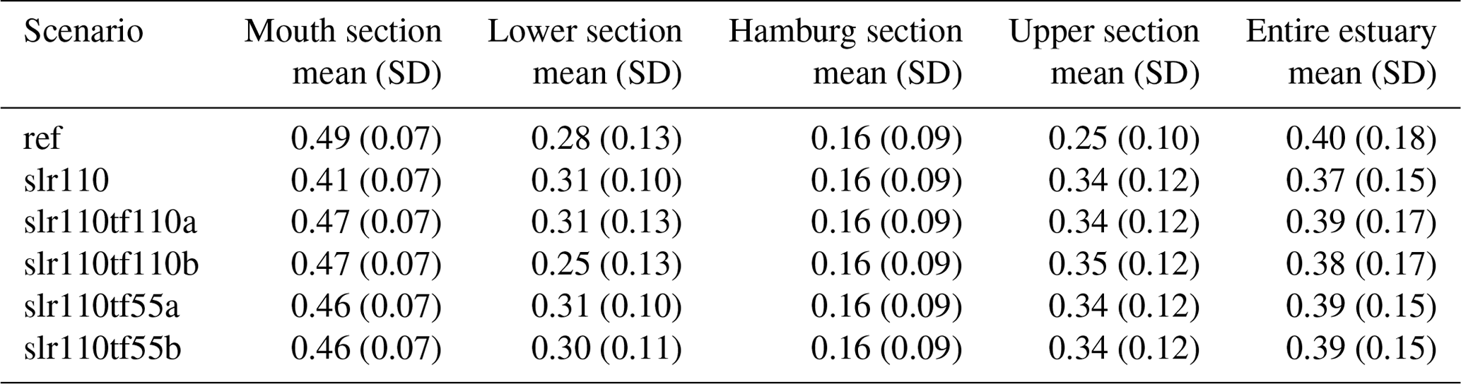
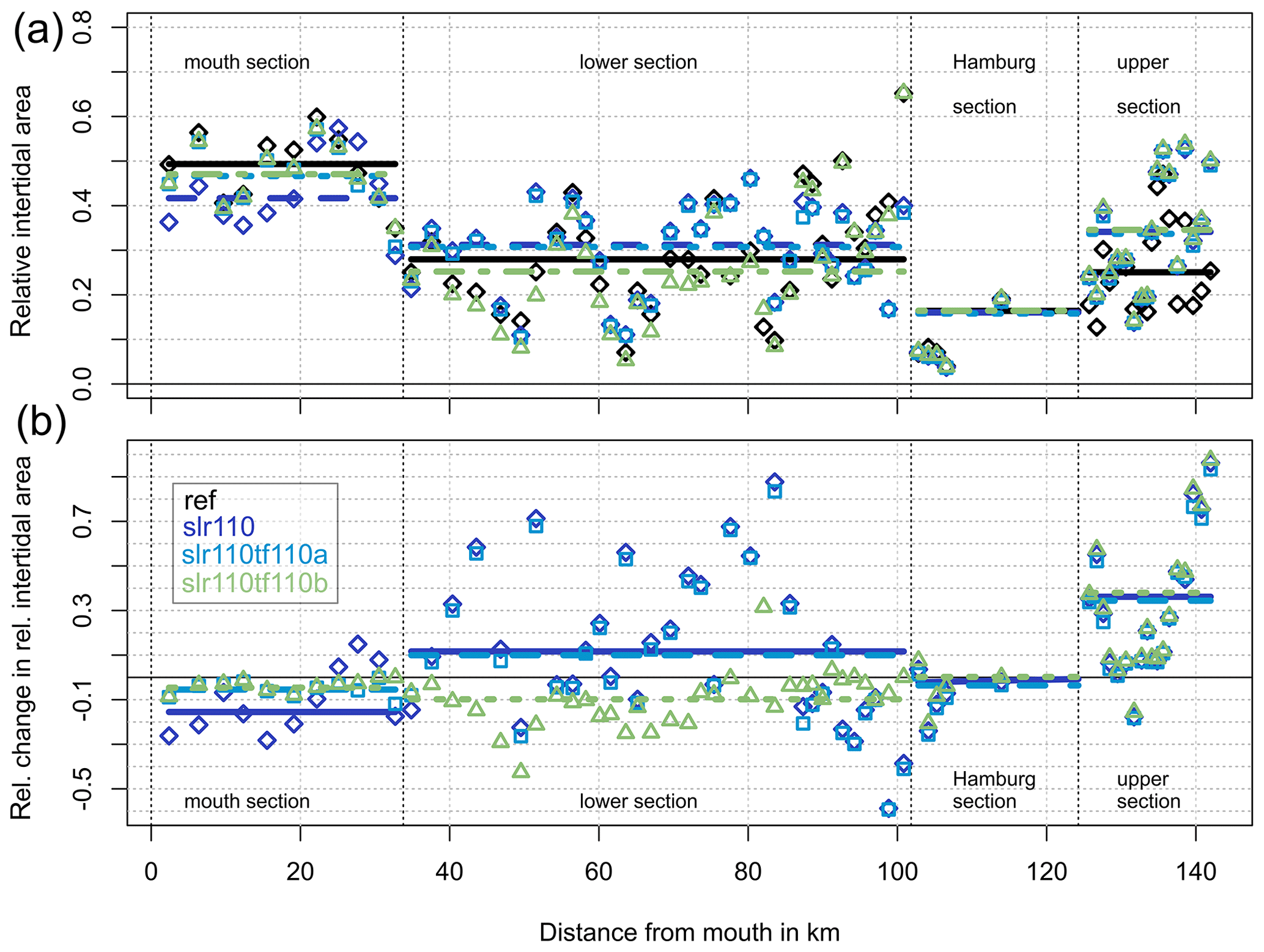
Figure 10Relative intertidal area (a) and relative change in relative intertidal area (b) in each control volume (markers) and section (lines) along the estuary for scenarios ref (black), slr110 (dark blue rhombuses), slr110tf110a (light blue squares) and slr110tf110b (green triangles). (The results of the scenarios slr110tf55a and slr110tf55b are not shown in the figure for better readability.)
The relative intertidal area ϙSint as well as the change in ϙSint strongly varies between the control volumes along the estuary. Due to SLR of 110 cm (slr110), ϙSint becomes smaller in the largest part of the mouth section (downstream of kilometre 25) and mostly increases in the lower (downstream of kilometre 85) and upper sections. Tidal flat elevation counteracts the changes in SLR in the sections where tidal flats are elevated (mouth section and lower section) and results in ϙSint close to the reference scenario for these sections.
The results show an increase in TR in the Elbe estuary because of SLR. They also reveal that tidal flat growth with SLR can either have no effect, or can decrease or increase TR relative to the isolated effect of SLR, depending on where and to what extent the tidal flats are elevated. Further analysis shows that the geometric parameters of the Elbe estuary change under the combined impact of SLR and tidal flat elevation. In the following section we will discuss the changes in the estuarine geometry and their possible causes. We will then go on to propose explanatory approaches for the changes in TR based on changes in geometry.
4.1 Convergence length
Our estimated value for the estuary's convergence length (La) in the reference condition is 46.5 km. This value lies in the same order of magnitude as the values estimated by Dronkers (2017) (42 km) and Savenije et al. (2008) (30 km) for the Elbe estuary. Scenario slr110 results in a significant decrease in La and therefore a stronger convergence of the Elbe estuary relative to the reference condition. In scenario slr110tf110a, upstream convergence weakens relative to slr110, which results in an La close to the reference condition.
A change in La is the result of differing changes in the cross-sectional area (A) along the estuary in the upstream direction, which are due to regional dissimilarity in cross-sectional geometry. As discussed in Friedrichs et al. (1990), changes in intertidal storage capacity, cross-sectional flow area and channel width due to SLR are strongly dependent on the gradient of the estuary banks. The model results correspondingly show a stronger increase in the cross-sectional flow area in the mouth section of the Elbe estuary where tidal flat areas (meaning low topographic gradient) are larger compared to other sections. It can therefore be assumed that the stronger convergence of A as a result of SLR is due to the decrease in the amount of relative intertidal area further upstream in the estuary (Fig. 10). This effect is sketched in Fig. 11. Tidal flat elevation decreases A regionally and seems to significantly counteract SLR-induced changes in convergence in scenario slr110tf110a but not in the other scenarios.
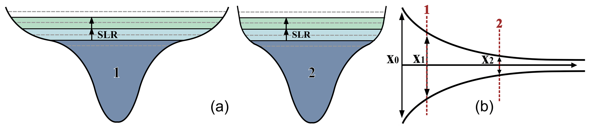
Figure 11Schematic of SLR in estuary cross-sections (a) with large (1) and small (2) SINT and schematic plan view of an estuary (b). The black lines in the cross-sections show the MW for a reference scenario (dark blue) and two SLR scenarios (light blue and light green).
4.2 Mean hydraulic depth
In the reference scenario, we derive a mean hydraulic depth averaged over the entire estuary (up to the weir in Geesthacht) of 7.0 m for ht (including intertidal area) and 9.2 m for hc (excluding intertidal area). In comparison, Savenije et al. (2008) listed a mean depth at MW of 7.0 m, increasing to 9.0 m further upstream for the Elbe estuary, and Dronkers (2016) listed a time-averaged channel depth of 10.0 m for the Elbe estuary. However, it is not clear how these numbers were derived.
Our simulation results for the SLR scenarios might be unexpected and counter-intuitive since they show that SLR of 110 cm does not, in general, cause an increase in mean hydraulic depth along the estuary. To the contrary, the mean hydraulic depth shows varying changes and even a decrease in some parts of the estuary for slr110 relative to the reference scenario. These differing changes in mean hydraulic depth along the estuary are caused by the varying topographic gradients of the control volumes. A decrease in hc due to SLR can be explained by an effect where the shallow areas next to the previous channels become part of the enlarged channels (Friedrichs et al., 1990); due to an elevated LW, some of the areas next to the channel that previously belonged to the intertidal zone can develop into subtidal areas and thus become part of the channel (Fig. 12). Because of the relatively small water depth in this new part of the channel, the hydraulic depth averaged over the channel cross-section can decrease. Moreover, elevated HW can cause the shallow previously supratidal areas to become intertidal areas (see Fig. 12), which explains the decrease in ht. However, if tidal flats are elevated with SLR in the model, this results in a regional increase in mean hydraulic depth relative to slr110 and relative to the reference condition in the Elbe estuary. Tidal flat elevation counteracts the abovementioned effect where shallow areas become part of the subtidal and intertidal cross-sections and this overall results in a greater mean hydraulic depth due to SLR in these scenarios.
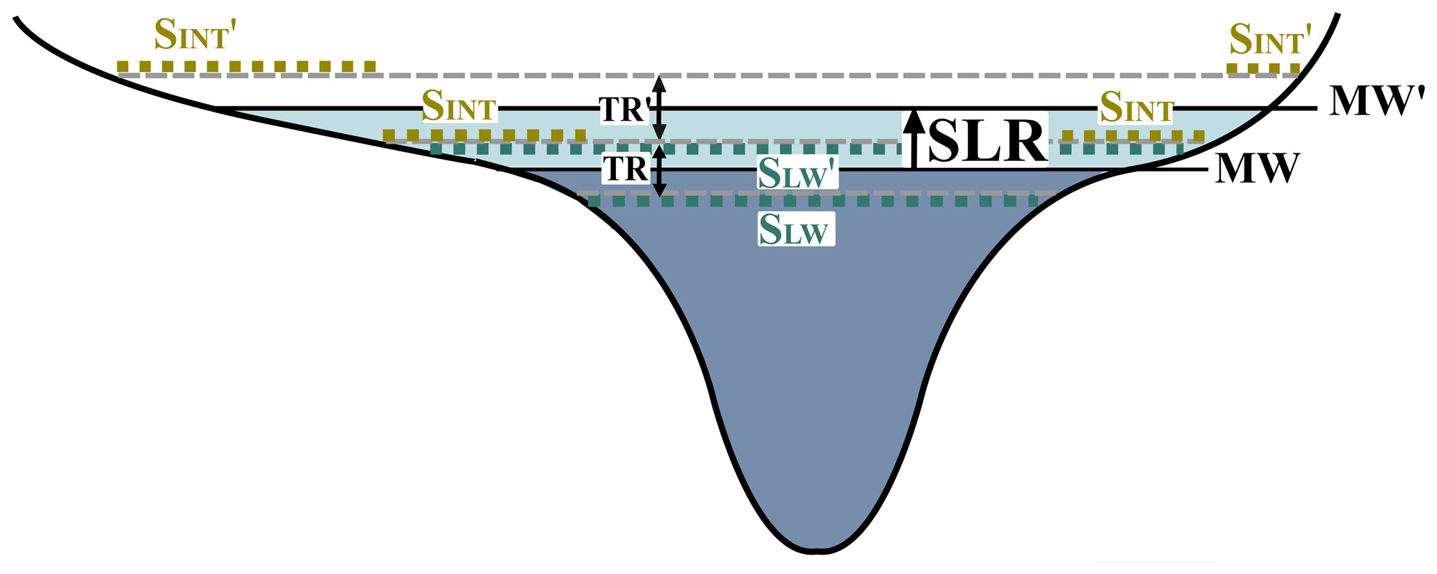
Figure 12Schematic of SLR in estuary cross-sections and the resulting changes in the intertidal area (SINT) for different topographic gradients between high water (HW) and low water (LW). The left side of the figure shows a low gradient; the right side shows a higher gradient. The black lines correspond to MW for the reference condition (dark blue) and SLR (light blue). All parameters with an apostrophe belong to the scenario with SLR. The dashed grey lines show HW and LW for both scenarios; the coloured dotted lines show SINT and SLW.
4.3 Relative intertidal area
For the reference condition, we analyse a mean ϙSINT of 0.4 for the entire estuary, which is slightly lower than the value of 0.5 derived by Dronkers (2016) for the Elbe estuary and in the range of 0.412 to 0 (decreasing in the upstream direction) given by Savenije et al. (2008). Note that Dronkers (2016) and Savenije et al. (2008) used a different form (ratio of width at HW to width at LW) and that these numbers are converted for comparability.
According to our simulation results, an SLR of 110 cm causes regionally, strongly and widely scattered changes in ϙSint along the estuary with a decrease in some control volumes and an increase in others. Tidal flat elevation counteracts these changes regionally. The varying changes along the estuary can be explained by the differing topographic gradients. In general, SLR can either cause an increase or decrease inSINT, or it causes no change at all, depending on the local topographic gradient above LW and a potential change in TR (see Fig. 12). An increase in SINT can result from previously supratidal areas (above old HW) becoming part of the SINT due to SLR (Dronkers, 2016), and/or it can be caused by an increased TR. A decrease in SINT can occur in tidal systems that are contained by dikes or restricted by a strong-gradient topography. In such cases, the size of previous SINT that becomes subtidal area (SLW) can be larger as a result of SLR than the size of a previously supratidal area that becomes SINT due to SLR (Dronkers, 2016) (see Fig. 12). However, a decrease in SINT can also be caused by a decrease in TR.
4.4 Changes in tidal range and explanatory approaches
The effects of the previously discussed changes in geometric parameters on tidal dynamics act simultaneously and can therefore counteract, outweigh or enhance each other in the resulting impact on TR. However, we want to point out correlations between the detected changes in geometry and in TR to find explanatory approaches for the latter.
SLR of 110 cm without topographic changes
The simulation results show an increased TR in the estuary in scenario slr110 relative to the reference condition. The analysis of the upstream convergence of the cross-sectional flow area (A) accordingly shows a significant increase in convergence in scenario slr110 relative to the reference condition. We assume this is the main reason for the increased TR in slr110, as the gradual convergence in width and depth causes an amplification of the tidal wave according to Green's law (1837) (Sect. 2.3.3). Averaged over the different sections, a decrease in ϙSINT in the mouth section and an increase further upstream are detected. These could contribute to or counteract the increase in TR respectively (Sect. 2.3.5). According to our analysis, SLR of 110 cm does not cause a general increase in mean hydraulic depth, but causes strongly varying changes along the estuary. Averaged over the sections, mean hydraulic depth remains approximately unchanged relative to the reference condition for the largest part of the estuary. In the Hamburg section and the upper section, a greater mean hydraulic depth is detected. The hydrodynamics in this upper part of the estuary are not fully dominated by the tide but are also highly influenced by discharge. We assume the strong increase in TR in these sections to be caused by an increase in tidal influence relative to discharge influence.
SLR of 110 cm with tidal flat elevation in Scenario A
In scenario slr110tf55a, TR is the same as in slr110. Accordingly, an analysis of convergence shows no significant changes compared to slr110. In contrast, if the tidal flats in Scenario A are elevated by 100 % with SLR (slr110tf110a), TR decreases relative to slr110 along the entire estuary. Our analysis accordingly shows a significant decrease in convergence for slr110tf110a compared to slr110, which might be the main reason for the decrease in TR. On average, the mouth section is characterised by an increase in both relative intertidal area and mean hydraulic depth, the impacts of which might counteract each other.
SLR of 110 cm with tidal flat elevation in Scenario B
In scenario slr110tf55b, TR strongly increases relative to SLR alone (scenario slr110) in the entire estuary, while in scenario slr110tf110b a decrease can be seen in the mouth section and an increase is observed further upstream. In both scenarios, a significant change in convergence relative to slr110 cannot be detected with a significance level of α=0.1. The average of ϙSINT in the lower section shows a decrease for scenario slr110tf110b compared to scenario slr110 which might partly explain the increase in TR. However, a notable decrease in slr110tf55b cannot be seen. Therefore, we assume that in the scenarios slr110tf55b and slr110tf110b the main reason for the increase in TR is the change in mean hydraulic depth, which increases as the tidal flats are elevated. In contrast to the scenarios where the tidal flats are only elevated in the mouth of the estuary, mean hydraulic depth increases in a much larger part of the estuary and is therefore most likely to have a stronger effect on TR. As mentioned in Sect. 2.3.4, changes in water depth influence frictional damping of a tidal wave due to energy dissipation, and they can also push a system closer to or further away from resonance. Whether the increase in TR due to increased mean hydraulic depth is mainly caused by a decrease in frictional damping or by a shift towards resonance is a question that needs further investigation.
4.5 Comparison to other studies
Seiffert and Hesser (2014) simulated the effects of 80 cm SLR without topographic changes in the Elbe estuary and found an increase in TR, which is in accordance with our results. Jordan et al. (2021) did not focus on the estuaries when investigating the effects of SLR and tidal flat elevation on tidal dynamics in the Wadden Sea. Nevertheless, their results show a slight increase in M2 amplitude in the Elbe estuary due to SLR of 80 cm without tidal flat elevation. They also show a much stronger increase when the tidal flats are elevated in the entire estuary, which qualitatively corresponds to our results. Du et al. (2018) analysed tidal response to SLR in different types of idealised estuaries and for different realistic estuaries in the USA. The authors point out the relevance of length, convergence and lateral bathymetry of estuaries for the resulting changes due to SLR. In contrast to our study, they tried to find explanatory approaches for the changes in realistic estuaries by matching their geometric characteristics to the different types of geometry of idealised estuaries (e.g. differences in length, convergence and cross-sectional bathymetric gradient), but they did not analyse the changes in geometry due to SLR. Without further evaluating, they mention the possible change in convergence characteristics under SLR conditions and spatially variable tidal response due to spatially variable lateral geometry (e.g. size of intertidal area).
4.6 Limitations
In our study, SLR-induced changes in tidal dynamics seaward of the German Bight model are neglected. Previous research by Jordan et al. (2021) shows large-scale changes in M2 amplitude in the North Sea due to SLR. Relating the results of Jordan et al. (2021) to our model boundary, we neglect changes in the M2 amplitude that are less than ±2 cm. We assume that this has no bearing on the key results of our study, which aims to improve system understanding of the changes in the Elbe estuary induced by SLR and tidal flat growth.
To reduce computational effort, the generation of wind waves as well as sediment and heat transport is not included in our model setup. Hence, potential changes in sediment dynamics, e.g. changes in the ETM (estuarine turbidity maximum) and their potential effect on tidal dynamics, are neglected. Furthermore, our investigation does not include potential future changes in river discharge into the Elbe estuary, as the discharge in the model is kept constant (600 m3 s−1).
We selected the SLR scenario of 110 cm with corresponding hypothetical tidal flat elevation scenarios which we analysed in detail. For scenarios with 55 cm SLR, we found qualitatively similar changes in maximum TR and therefore assume similar alterations in estuarine geometry. However, to ensure that our results are in principle applicable to other scenarios than an SLR of 110 cm, it would be necessary to simulate a range of several SLR scenarios with their corresponding tidal flat growth scenarios and analyse the changes in tidal dynamics and estuarine geometry for each of them.
The aim of this study is to gain a better system understanding of the Elbe estuary in the context of sea level rise (SLR) and accompanying topographic changes. Using a three-dimensional hydrodynamic numerical model of the German Bight, we investigated the effect of SLR and several simplified tidal flat elevation scenarios on the tidal dynamics in the Elbe estuary. With SLR values of 55 and 110 cm, the simulation results reveal an increase in the tidal range (TR) in the estuary. The results further show that potential tidal flat growth can either have no effect or cause a decrease or increase in TR relative to the isolated effect of SLR, depending on the location and extent of tidal flat elevation. Further analysis of the simulation results was conducted for the scenarios with 110 cm SLR. We analysed three geometric parameters of the estuary to find indications explaining the causes of changes in TR: convergence of cross-sectional flow area, mean hydraulic depth and relative intertidal area.
The results reveal an increase in the upstream convergence of the cross-sectional flow area in the estuary which is solely due to the SLR of 110 cm. This effect is counteracted in the tidal flat growth scenario slr110tf110a where the tidal flats in the mouth of the estuary grow to 100 % with SLR. Our analyses suggest that these changes in estuarine convergence might be the main reason for the respective increase and decrease in TR in these scenarios. Additionally, we find that SLR alone does not cause a general increase in mean hydraulic depth along the estuary but causes almost no changes or even a decrease in large parts of the estuary. However, if the tidal flats are elevated in combination with SLR, mean hydraulic depth in the elevated regions increases. Therefore, an elevation of the tidal flats in the entire estuary (scenarios slr110tf55b and slr110tf110b) causes an increase in mean hydraulic depth in a large part of the estuary. This is probably the main reason for the increase in TR in these scenarios relative to SLR alone. The results of this study show that the future development of TR in the Elbe estuary depends not only on future SLR but also on the development of tidal flats. The results further show varying changes in estuarine geometry for the different scenarios, which can explain the differing changes in TR and improve understanding of the system in the context of SLR.
We are able to use the detected changes in estuarine geometry to find qualitative explanatory approaches for the changes in TR. Therefore, the analysis of simplified parameters of estuarine geometry, originally developed in studies with analytical models, has proven useful for understanding and interpreting the results of advanced numerical models. However, to further quantify and separate the influence of the changes in each analysed geometric parameter on TR, an analytical model of the estuary could be used with the abovementioned geometric parameters as input values. For further generalised understanding, it would be helpful to conduct similar analyses in other estuaries. We are therefore planning to carry out similar investigations for other estuaries in the German Bight in future studies.
This study focuses on the changes occurring in parameters of the vertical tide – especially TR – due to SLR and potential accompanying tidal flat growth scenarios. Future studies could additionally analyse changes in current velocities, tidal asymmetry, sediment transport and salt intrusion, as they are of concern regarding sediment management and other human activities in and around the estuary as well as for biodiversity. The findings of this study are helpful for the development of adaptation measures in the Elbe estuary. The results underline the importance of taking topographic changes into account when analysing the dependence of tidal dynamics in estuaries on future SLR, which is necessary, for example, as a basis for adapting infrastructure along the waterway. This study demonstrates that SLR and potential corresponding tidal flat elevation scenarios can cause changes in tidal dynamics which are strongly dependent on the individual topography of an estuary and the corresponding change in estuarine geometry.
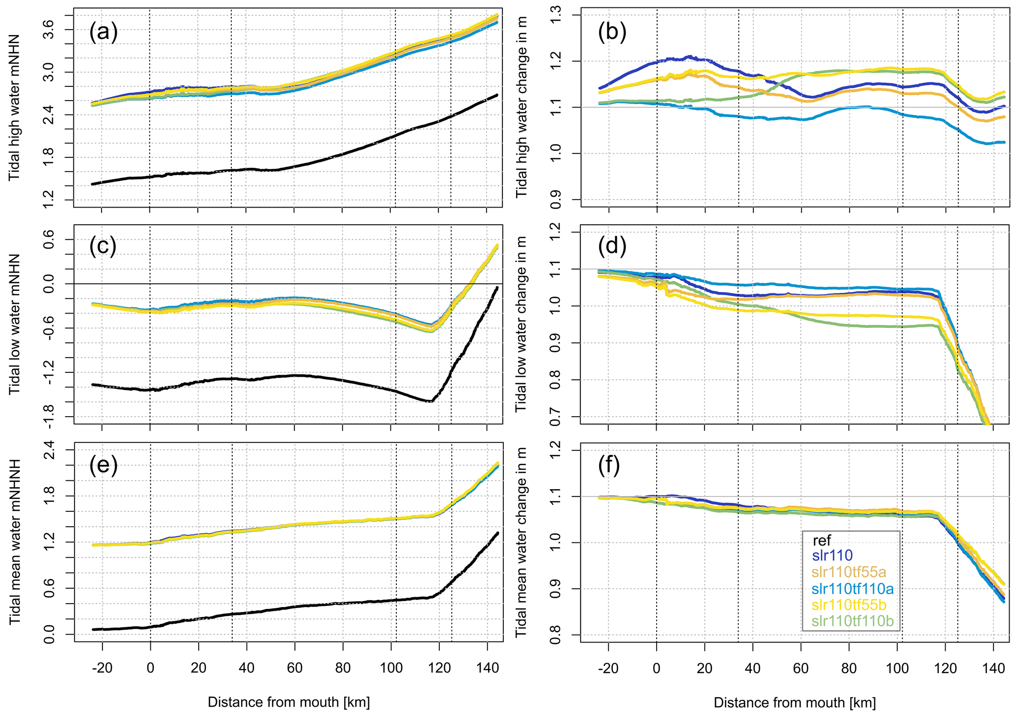
Figure A1HW (a), LW (c) and MW (e) relative to mNHN (German vertical datum) and changes in these parameters relative to reference condition (in m) (b, d, and f) along the estuary profile analysed for a spring–neap cycle for the scenarios ref (black), slr110 (dark blue), slr110tf55a (orange), slr110tf110a (light blue), slr110tf55b (yellow) and slr110tf110b (green).
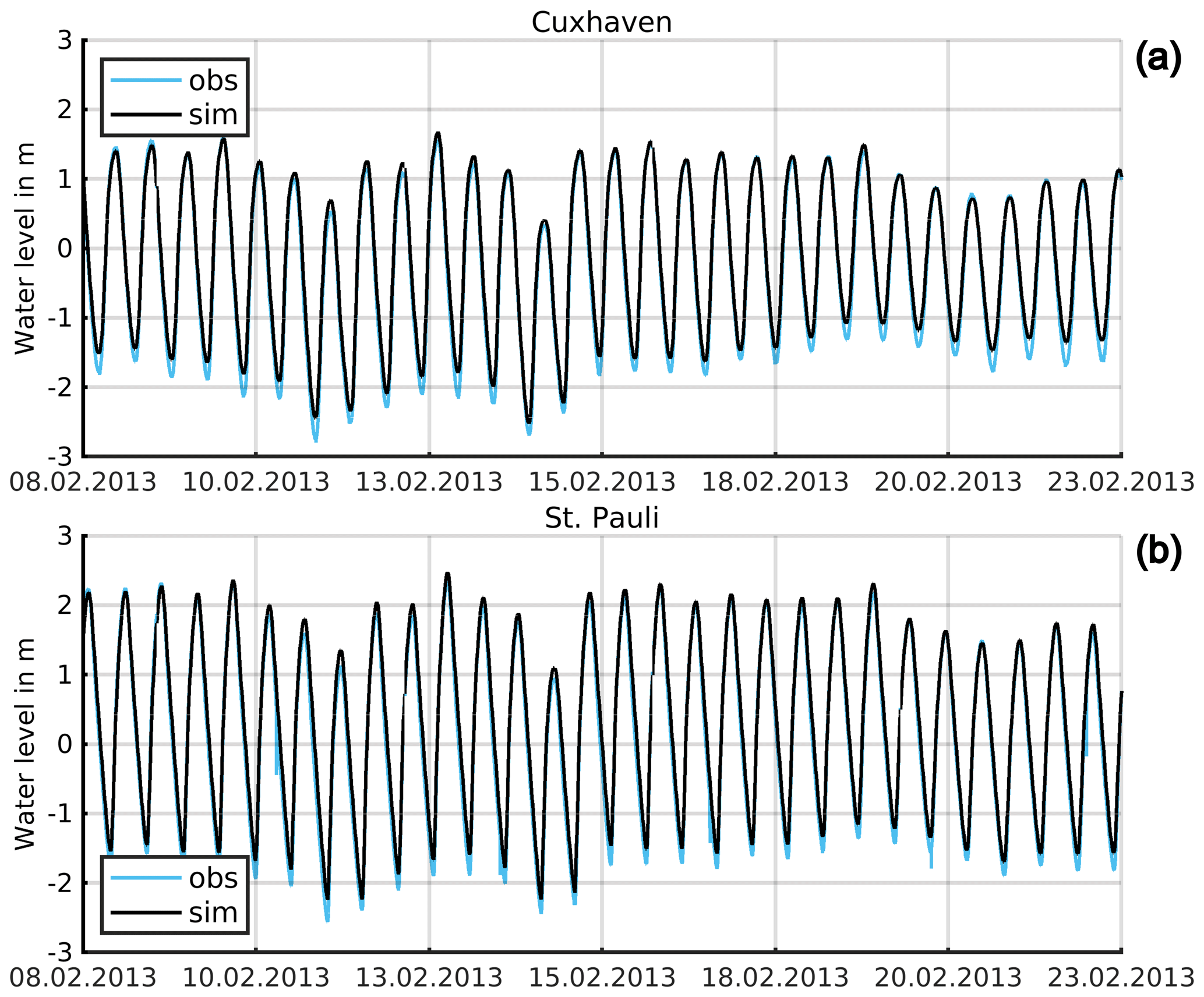
Figure A2Simulated (black) and observed (blue) water levels at the stations in Cuxhaven (a) and St Pauli (b).
The raw simulation results as well as the results from the analysis are available, on request, from the corresponding author. Water level and river discharge measurement data can be accessed from the open data portal of the Federal Waterways and Shipping Administration (https://www.kuestendaten.de/DE/Services/Messreihen_Dateien_Download/Download_Zeitreihen_node.html, WSV, 2022). The COSMO-REA6 data used for the atmospheric forcing of our model can be accessed from DWD (2022, https://data.opendatascience.eu/geonetwork/srv/api/records/4d6f6090-c242-454b-9224-1151f7ae2823).
TFM worked on the simulations, analysis, figures and interpretation. TFM also wrote the article with contributions from RS. JK, PF and RS were involved as scientific experts, supervised the study and gave input for writing and revision of the paper.
The contact author has declared that none of the authors has any competing interests.
Publisher's note: Copernicus Publications remains neutral with regard to jurisdictional claims made in the text, published maps, institutional affiliations, or any other geographical representation in this paper. While Copernicus Publications makes every effort to include appropriate place names, the final responsibility lies with the authors.
This article is part of the special issue “Oceanography at coastal scales: modelling, coupling, observations, and applications”. It is not associated with a conference.
We thank the German Federal Ministry for Digital and Transport for funding this work as part of the Network of Experts. Furthermore, we thank our coworkers at the Federal Waterways Engineering and Research Institute in Hamburg for their continuous support. Special thanks go to Elisabeth Rudolph, Caroline Rasquin, Ingo Hache, Norbert Winkel, Benno Wachler and Ralf Fritzsch for their support and inspiring discussions and to Günther Lang for the development of the employed postprocessing tools. We also thank two anonymous reviewers for their careful reading and valuable suggestions, which led to a substantial improvement in the manuscript.
This study was funded by the German Federal Ministry for Digital and Transport (BMDV) in the context of the BMDV Network of Experts.
This paper was edited by Davide Bonaldo and reviewed by two anonymous referees.
Aubrey, D. G. and Speer, P. E.: A study of non-linear tidal propagation in shallow inlet/estuarine systems. Part I: Observations, Estuar. Coast. Shelf S., 21, 185–205, https://doi.org/10.1016/0272-7714(85)90096-4, 1985.
Baty, F., Ritz, C., Charles, S., Brutsche, M., Flandrois, J.-P., and Delignette-Muller, M.-L.: A Toolbox for Nonlinear Regression in R The Package nlstools, J. Stat. Softw., 66, 1–21, https://doi.org/10.18637/jss.v066.i05, 2015.
BAW: Analysis of calculated results, http://wiki.baw.de/en/index.php/Analysis_of_Calculated_Results (last access: 8 November 2023), 2010.
Becherer, J., Hofstede, J., Gräwe, U., Purkiani, K., Schulz, E., and Burchard, H.: The Wadden Sea in transition – consequences of sea level rise, Ocean Dynam., 68, 131–151, https://doi.org/10.1007/s10236-017-1117-5, 2018.
Benninghoff, M. and Winter, C.: Recent morphologic evolution of the German Wadden Sea, Sci. Rep.-UK, 9, 9293, https://doi.org/10.1038/s41598-019-45683-1, 2019.
Boehlich, M. J. and Strotmann, T.: Das Elbeästuar, in: Die Küste 87, Kuratorium für Forschung im Küsteningenieurwesen (KFKI), https://doi.org/10.18171/1.087106, 2019.
Bollmeyer, C., Keller, J. D., Ohlwein, C., Wahl, S., Crewell, S., Friederichs, P., Hense, A., Keune, J., Kneifel, S., Pscheidt, I., Redl, S., and Steinke, S.: Towards a high-resolution regional reanalysis for the European CORDEX domain, Q. J. Roy. Meteor. Soc., 141, 1–15, https://doi.org/10.1002/qj.2486, 2015.
Klein, H., Frohse, A., and Schulz, A.: Salzgehalt, 136–146, in: Nordseezustand 2008–2011, Berichte des BSH, Vol. 54, 311 pp., Bundesamt für Seeschifffahrt und Hydrographie, Hamburg and Rostock, 2016.
Carrère, L., Lyard, F., Cancet, M., Guillot, A., and Roblou, L.: FES 2012: A New Global Tidal Model Taking Advantage of Nearly 20 Years of Altimetry, in: 20 Years of Progress in Radar Altimatry, Venice, 24–29 September, ISBN 978-92-9221-274-2, 2013.
Casulli, V.: A high-resolution wetting and drying algorithm for free-surface hydrodynamics, Int. J. Numer. Meth. Fl., 60, 391–408, https://doi.org/10.1002/fld.1896, 2008.
Casulli, V. and Walters, R. A.: An unstructured grid, three-dimensional model based on the shallow water equations, Int. J. Numer. Meth. Fl., 32, 331–348, 2000.
Dissanayake, D. M. P. K., Ranasinghe, R., and Roelvink, J. A.: The morphological response of large tidal inlet/basin systems to relative sea level rise, Climatic Change, 113, 253–276, https://doi.org/10.1007/s10584-012-0402-z, 2012.
Dronkers, J.: Dynamics of Coastal Systems, 2nd Edn., in: Advanced Series on Ocean Engineering, Vol. 41, World Scientific, Singapore, https://doi.org/10.1142/9818, 2016.
Dronkers, J.: Convergence of estuarine channels, Cont. Shelf Res., 144, 120–133, https://doi.org/10.1016/j.csr.2017.06.012, 2017.
Du, J., Shen, J., Zhang, Y. J., Ye, F., Liu, Z., Wang, Z., Wang, Y. P., Yu, X., Sisson, M., and Wang, H. V.: Tidal Response to Sea-Level Rise in Different Types of Estuaries: The Importance of Length, Bathymetry, and Geometry, Geophys. Res. Lett., 45, 227–235, https://doi.org/10.1002/2017GL075963, 2018.
DWD: Regional Reanalysis COSMO-REA6, DWD [data set], https://data.opendatascience.eu/geonetwork/srv/api/records/4d6f6090-c242-454b-9224-1151f7ae2823 (last access: 13 March 2024), 2022.
Fox-Kemper, B., Hewitt, H. T., Xiao, C., Aðalgeirsdóttir, G., Drijfhout, S. S., Edwards, T. L., Golledge, N. R., Hemer, M., Kopp, R. E., Krinner, G., Mix, A., Notz, D., Nowicki, S., Nurhati, I. S., Ruiz, L., Sallée, J.-B., Slangen, A., and Yu, Y.: Ocean, Cryosphere and Sea Level Change, in: Climate Change 2021: The Physical Science Basis. Contribution of Working Group I to the Sixth Assessment Report of the Intergovernmental Panel on Climate Change, edited by: Masson-Delmotte, V., Zhai, P., Pirani, A., Connors, S. L., Péan, C., Berger, S., Caud, N., Chen, Y., Goldfarb, L., Gomis, M. I., Huang, M., Leitzell, K., Lonnoy, E., Matthews, J. B. R., Maycock, T. K., Waterfield, T., Yelekçi, O., Yu, R., and Zhou, B., Cambridge University Press, Cambridge, United Kingdom and New York, NY, USA, 1211–1362, https://doi.org/10.1017/9781009157896.011., 2021.
Friedrichs, C. T.: Barotropic tides in channelized estuaries, in: Contemporary Issues in Estuarine Physics, edited by: Valle-Levinson, A., Cambridge University Press, 27–61, https://doi.org/10.1017/CBO9780511676567, 2010.
Friedrichs, C. T.: Tidal Flat Morphodynamics: A Synthesis, Treatise on Estuarine and Coastal Science, 3, 137–170, https://doi.org/10.1016/B978-0-12-374711-2.00307-7, 2011.
Friedrichs, C. T. and Aubrey, D. G.: Tidal propagation in strongly convergent channels, J. Geophys. Res., 99, 3321, https://doi.org/10.1029/93JC03219, 1994.
Friedrichs, C. T., Aubrey, D. G., and Speer, P. E.: Impacts of Relative Sea-level Rise on Evolution of Shallow Estuaries, in: Residual Currents and Long-term Transport. Coastal and Estuarine Studies, edited by: Cheng, R. T., Vol. 38, Springer, New York, NY, https://doi.org/10.1007/978-1-4613-9061-9_9, 1990.
Garner, G. G., Hermans, T., Kopp, R. E., Slangen, A. B. A., Edwards, T. L., Levermann, A., Nowikci, S., Palmer, M. D., Smith, C., Fox-Kemper, B., Hewitt, H. T., Xiao, C., Aðalgeirsdóttir, G., Drijfhout, S. S., Golledge, N. R., Hemer, M., Krinner, G., Mix, A., Notz, D., Nowicki, S., Nurhati, I. S., Ruiz, L., Sallée, J.-B., Yu, Y., Hua, L., Palmer, T., and Pearson, B.: IPCC AR6 Sea-Level Rise Projections, Version 20210809, https://podaac.jpl.nasa.gov/announcements/2021-08-09-Sea-level-projections-from-the-IPCC-6th-Assessment-Report (last access: 16 May 2022), Zenodo [data set], https://doi.org/10.5281/zenodo.5914709, 2021.
Garrett, C., Keeley, J. R., and Greenberg, D. A.: Tidal mixing versus thermal stratification in the Bay of Fundy and gulf of Maine, Atmosphere-Ocean, 16, 403–423, https://doi.org/10.1080/07055900.1978.9649046, 1978.
Gisen, J.: Prediction in Ungauged Estuaries, PhD thesis, TU Delft, https://doi.org/10.4233/uuid:a4260691-15fb-4035-ba94-50a4535ef63d, 2015.
Green, G.: On the Motion of Waves in a variable Canal of small Depth and Width, Transactions of the Cambridge Philosophical Society, 6, 457–462, 1837.
Holleman, R. C. and Stacey, M. T.: Coupling of Sea Level Rise, Tidal Amplification, and Inundation, J. Phys. Oceanogr., 44, 1439–1455, https://doi.org/10.1175/JPO-D-13-0214.1, 2014.
HTG: Empfehlungen des Arbeitsausschusses “Ufereinfassungen” Häfen und Wasserstraßen EAU 2020 (incl. e-book as PDF), 12th edn., Ernst Wilhelm & Sohn, Berlin, 700 pp., ISBN 9783433033166, 2020.
Jay, D. A.: Green's law revisited: Tidal long-wave propagation in channels with strong topography, J. Geophys. Res., 96, 20585, https://doi.org/10.1029/91JC01633, 1991.
Jordan, C., Visscher, J., and Schlurmann, T.: Projected Responses of Tidal Dynamics in the North Sea to Sea-Level Rise and Morphological Changes in the Wadden Sea, Front. Mar. Sci., 8, 40171, https://doi.org/10.3389/fmars.2021.685758, 2021.
Kernkamp, H. W. J., van Dam, A., Stelling, G. S., and de Goede, E. D.: Efficient scheme for the shallow water equations on unstructured grids with application to the Continental Shelf, Ocean Dynam., 61, 1175–1188, https://doi.org/10.1007/s10236-011-0423-6, 2011.
Khojasteh, D., Glamore, W., Heimhuber, V., and Felder, S.: Sea level rise impacts on estuarine dynamics: A review, Sci Total Environ., 780, 146470, https://doi.org/10.1016/j.scitotenv.2021.146470, 2021.
Kloepper, S., Baptist, M. J., Bostelmann, A., Busch, J. A., Buschbaum, C., Gutow, L., Janssen, G., Jensen, K., Jørgensen, H. P., de Jong, F., Lüerßen, G., Schwarzer, K., Strempel, R., and Thieltges, D.: Wadden Sea Quality Status Report, https://qsr.waddensea-worldheritage.org/?_gl=1*1lhw65f*_ga*
MTk4MTkxMDczLjE2OTcwMTU4Njc.*_ga_W7PEFV8FMW
*MTY5NzAxNTg2Ni4xLjAuMTY5NzAxNTg2Ni4wLjAuMA. (last access: 11 October 2023), 2017.
Lang, G.: Analyse von HN-Modell-Ergebnissen im Tidegebiet, Mitteilungsblatt der Bundesanstalt für Wasserbau, 101–108, https://hdl.handle.net/20.500.11970/102640 (last access: 13 March 2024), 2003.
Rasquin, C., Seiffert, R., Wachler, B., and Winkel, N.: The significance of coastal bathymetry representation for modelling the tidal response to mean sea level rise in the German Bight, Ocean Sci., 16, 31–44, https://doi.org/10.5194/os-16-31-2020, 2020.
Ray, R. D.: A Global Ocean Tide Model from TOPEX/POSEIDON Altimetry: GOT99.2, NASA, https://nla.gov.au/nla.cat-vn4150344 (last access: 13 March 2024), 1999.
Savenije, H. H. G.: Salinity and Tides in Alluvial Estuaries: Second Completely Revised Edition, version 2.6, https://hubertsavenije.files.wordpress.com/2022/04/salinityandtides2_6.pdf (last access: 13 March 2024), 2012.
Savenije, H. H. G., Toffolon, M., Haas, J., and Veling, E. J. M.: Analytical description of tidal dynamics in convergent estuaries, J. Geophys. Res., 113, C10025, https://doi.org/10.1029/2007JC004408, 2008.
Sehili, A., Lang, G., and Lippert, C.: High-resolution subgrid models: Background, grid generation, and implementation, Ocean Dynam., 64, 519–535, https://doi.org/10.1007/s10236-014-0693-x, 2014.
Seiffert, R. and Hesser, F.: Investigating Climate Change Impacts and Adaptation Strategies in German Estuaries, Die Küste, 81, 551–563, 2014.
Sievers, J., Rubel, M., and Milbradt, P.: EasyGSH-DB: Bathymetrie (1996–2016), Bundesanstalt für Wasserbau [data set], https://doi.org/10.48437/02.2020.K2.7000.0002, 2020.
Simpson, J. H. and Hunter, J. R.: Fronts in the Irish Sea, Nature, 250, 404–406, https://doi.org/10.1038/250404a0, 1974.
Smith, S. D. and Banke, E. G.: Variantion of the surface drag coefficient with wind speed, Q. J. Roy. Meteor. Soc., 101, 656–673, 1975.
Song, D., Wang, X. H., Zhu, X., and Bao, X.: Modeling studies of the far-field effects of tidal flat reclamation on tidal dynamics in the East China Seas, Estuar. Coast. Shelf S., 133, 147–160, https://doi.org/10.1016/j.ecss.2013.08.023, 2013.
Talke, S. A. and Jay, D. A.: Changing Tides: The Role of Natural and Anthropogenic Factors, Annu. Rev. Mar. Sci., 12, 121–151, https://doi.org/10.1146/annurev-marine-010419-010727, 2020.
van der Wegen, M.: Numerical modeling of the impact of sea level rise on tidal basin morphodynamics, J. Geophys. Res.-Earth, 118, 447–460, https://doi.org/10.1002/jgrf.20034, 2013.
van Rijn, L. C.: Analytical and numerical analysis of tides and salinities in estuaries; part I: tidal wave propagation in convergent estuaries, Ocean Dynam., 61, 1719–1741, https://doi.org/10.1007/s10236-011-0453-0, 2011.
Wachler, B., Seiffert, R., Rasquin, C., and Kösters, F.: Tidal response to sea level rise and bathymetric changes in the German Wadden Sea, Ocean Dynam., 70, 1033–1052, https://doi.org/10.1007/s10236-020-01383-3, 2020.
Willmott, C. J., Ackleson, S. G., Davis, R. E., Feddema, J. J., Klink, K. M., Legates, D. R., O'Donnell, J., and Rowe, C. M.: Statistics for the evaluation and comparison of models, J. Geophys. Res., 90, 8995, https://doi.org/10.1029/JC090iC05p08995, 1985.
Winterwerp, J. C. and Wang, Z. B.: Man-induced regime shifts in small estuaries – I: theory, Ocean Dynam., 63, 1279–1292, https://doi.org/10.1007/s10236-013-0662-9, 2013.
WSV: Zentrales Datenmanagement (ZDM): Küstendaten, WSV [data set], https://www.kuestendaten.de/DE/Services/Messreihen_Dateien_Download/Download_Zeitreihen_node.html (last access: 15 May 2023), 2022.
Zhou, Z., Coco, G., Townend, I., Gong, Z., Wang, Z., and Zhang, C.: On the stability relationships between tidal asymmetry and morphologies of tidal basins and estuaries, Earth Surf. Proc. Land., 43, 1943–1959, https://doi.org/10.1002/esp.4366, 2018.
Zijl, F.: An application of Delft3D Flexible Mesh for operational water-level forecasting on the Northwest European Shelf and North Sea (DCSMv6), Deltares, NGHS Symposium, Delft Software Days, 5 November 2014, https://de.slideshare.net/Delft_Software_Days/dsdint-2014-symposium-next-generation-hydro-software-nghs-north-sea-firmijn-zijl-deltares (last access: 13 March 2024), 2014.
Zijl, F., Verlaan, M., and Gerritsen, H.: Improved water-level forecasting for the Northwest European Shelf and North Sea through direct modelling of tide, surge and non-linear interaction, Ocean Dynam., 63, 823–847, https://doi.org/10.1007/s10236-013-0624-2, 2013.
Zijl, F., Sumihar, J., and Verlaan, M.: Application of data assimilation for improved operational water level forecasting on the northwest European shelf and North Sea, Ocean Dynam., 65, 1699–1716, https://doi.org/10.1007/s10236-015-0898-7, 2015.