the Creative Commons Attribution 4.0 License.
the Creative Commons Attribution 4.0 License.
 | 19 Feb 2024
Salt intrusion dynamics in a well-mixed sub-estuary connected to a partially to well-mixed main estuary
Zhongyuan Lin
Guang Zhang
Huazhi Zou
Salt intrusion in estuaries has been exacerbated by climate change and human activities. Previous studies have primarily focused on salt intrusion in the mainstem of estuaries, whereas those in sub-estuaries (those that branch off their main estuaries) have received less attention. During an extended La Niña event from 2021 to 2022, a sub-estuary (the East River estuary) alongside the Pearl River estuary, China, experienced severe salt intrusions, posing a threat to the freshwater supply in the surrounding area. Observations revealed that maximum salinities in the main estuary typically preceded spring tides, exhibiting significant asymmetry in salinity rise and fall over a fortnightly timescale. In contrast, in the upstream region of the sub-estuary, the variation in salinity was in phase with that of the tidal range, and the rise and fall of the salinity were more symmetrical.
Inspired by these observations, we employed idealized numerical models and analytical solutions to investigate the underlying physics behind these behaviors. It was discovered that under normal dry conditions (with a river discharge of 1500 m3 s−1 at the head of the main estuary), the river–tide interaction and change in horizontal dispersion accounted for the in-phase relationship between the salinity and tidal range in the upstream region of the sub-estuary. Under extremely dry conditions (i.e., a river discharge of 500 m3 s−1 at the head of the main estuary), salinity variations were in phase with those of the tidal range in the middle as well as the upstream region of the sub-estuary. The variation in salinity in the main estuary along with those in salt dispersion and freshwater influx inside the sub-estuary collectively influenced salinity variation in the well-mixed sub-estuary. These findings have important implications for water resource management and salt intrusion prevention in the catchment area.
- Article
(5974 KB) - Full-text XML
-
Supplement
(874 KB) - BibTeX
- EndNote


Salt intrusion in estuaries has emerged as an increasingly significant environmental issue, as it contaminates water quality, restricts freshwater supply, and affects the biota's habitat in estuaries (Payo-Payo et al., 2022). The severity of salt intrusion in estuaries has been further exacerbated by both climate change and anthropogenic activities. Climate change has led to more severe droughts in various regions worldwide (Spinoni et al., 2014), resulting in reduced freshwater flow from upstream watershed basins into estuaries. In turn, this has intensified salt intrusion in these areas. Additionally, sea level rise has been identified as a contributing factor to this phenomenon (e.g., Hong et al., 2020). Human activities, including dam construction in the watershed, channel dredging, and land reclamation in estuaries, have caused reductions in river inflow, channel deepening, and enhanced convergence of estuarine geometry, all of which favor an increase in salt intrusion (e.g., Ralston and Geyer, 2019).
Salt intrusion in estuaries is the result of landward salt transport, which consists of steady shear and tidal oscillatory transport (MacCready and Geyer, 2010). The combination of estuarine circulation and salinity stratification induces a steady shear when averaged in a tidal cycle. Tidal oscillatory transport is generated by tidal pumping such as the jet-sink flow for an inlet (Stommel and Farmer, 1952), tidal trapping with a side embayment (Okubo, 1973), tidal shear dispersion by the vertical shears of current and mixing (Bowden, 1965), tidal straining (Simpson et al., 1990), and chaotic stirring (Zimmerman, 1986).
In general, for a partially mixed estuary in which the steady shear dominates the landward salt transport, the salt intrusion is strongest during neap tides and weakest during spring tides under steady-state conditions, meaning that the change in salinity is out of phase with that in the tidal range. However, for a well-mixed and/or a salt wedge estuary, in which the tidal dispersion is the dominant contributor to landward salt transport, the salt intrusion is strongest during spring tides and weakest during neap tides, signifying that the salinity variation is in phase with the tidal range (Ralston et al., 2010). These steady-state situations are altered by the unsteadiness of external forcing and the adjustment of estuaries to the changing forcings (Chen, 2015, and references therein). In general, when the internal timescale of an estuary, which is defined as the time needed for a water parcel from the upstream area to travel through the estuary by river-induced flow, is shorter than the external timescale, which is often the spring–neap tidal cycle, the salinity variation in an estuary can keep pace with the change in tidal forcing and reaches steady state. However, when the internal timescale is longer than the external timescale, the salt intrusion can hardly reach the steady state, and there exists a phase shift between the salt intrusion and tidal range, such as in the Modaomen Estuary (Gong and Shen, 2011) and the Hudson River (Bowen and Geyer, 2003).
Previous studies on salt intrusion have primarily focused on main estuaries, where freshwater discharge empties into the estuarine waterbody at the estuary head and is profoundly diluted by the seawater from the ocean. However, there has been relatively less research on salinity dynamics specifically in tidal creeks or sub-estuaries, i.e., those that are located beside their main estuary. It is worth noting that larger estuaries often possess sub-estuaries or tidal creeks, as highlighted by Uncles and Stephens (2010). Sub-estuaries branch off the stem of their main estuary and exhibit behavior that is partially dependent on processes acting within the main estuary. Haywood et al. (1982) described the importance of conditions at the confluence of the York River sub-estuary and the Chesapeake Bay to salinity stratification within the sub-estuary. Uncles and Stephens (2010) investigated the salinity dynamics in a sub-estuary (Tavy) connected to the main estuary (Tamar, UK). They noted that the tidal range had a limited effect on the salinity in the sub-estuary. Yellen et al. (2017) examined the sediment dynamics in a side embayment of the main estuary of Connecticut, USA, and found that salinity intrusion from the main estuary enhanced sediment trapping inside the sub-estuary.
The previous studies on sub-estuary salt dynamics have mainly focused on examining salinity variabilities and water column stratification, as exemplified by the work of Haywood et al. (1982). Some investigations have also explored the influence of river discharge from the heads of the main estuary and sub-estuary, as well as the impact of winds, as discussed by Uncles and Stephens (2010). However, there remains a knowledge gap regarding how the salt dynamics in the main estuary affect those in the sub-estuary as well as how the interaction between river flow and tides influences salinity variations in the sub-estuary. Regarding the river–tide interaction, here we focus on how tides affect river flow through mechanisms such as nonlinear bottom friction and advective terms in the momentum equation, as outlined by Buschman et al. (2009), whereas the effect of river flow on tidal propagation will not be explored.
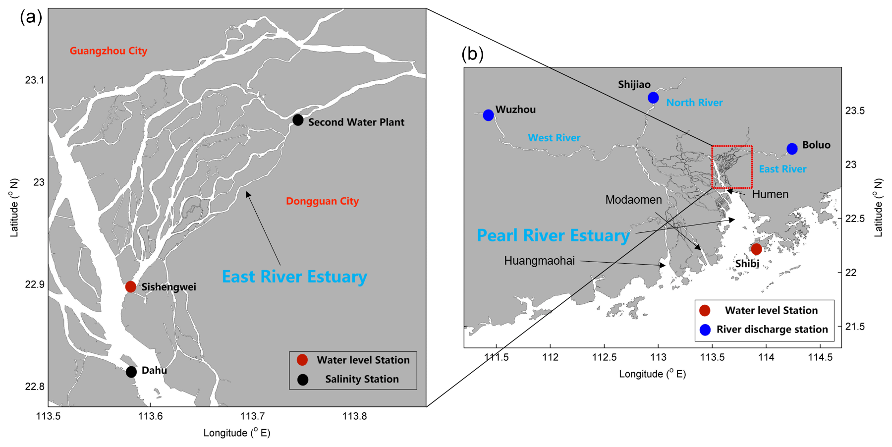
Figure 1(a) The East River estuary. (b) Map of the Pearl River Delta and the locations of hydrological and water level stations.
In 2021, under the influence of a La Niña event, the precipitation in the Pearl River Delta (PRD) area (Fig. 1), China, was extremely low, and the salt intrusion was very severe, which posed a great threat to the freshwater supply in the region, especially during winter months (December to February). Alongside the Pearl River estuary (PRE), a sub-estuary of the East River estuary (Fig. 1), also experienced strong salt intrusion and heavily impacted the water supply to the city of Dongguan, home to a population of 10 million people. This shortage of freshwater became a significant concern for the surrounding people, especially during the Spring Festival, the Chinese Lunar New Year.
The present work has two objectives: (a) to investigate the characteristics of salt intrusion in a well-mixed sub-estuary by analyzing observation data – the characteristics include spatiotemporal variations in salt intrusion and their relationship with river flow and tidal range; (b) to explore the underlying physics behind salt intrusion in the sub-estuary, such as the impacts of salt dynamics in the main estuary, and the river–tide interaction inside the sub-estuary. To achieve the above goals, we first collected and analyzed observational data of salt intrusion at the East River estuary. Then we utilized an idealized configuration for numerical model investigation. Two numerical model experiments with mean and extremely low river discharges in dry seasons in the main estuary, respectively, were conducted to identify the relevant mechanisms for the variability in salt intrusion in the sub-estuary. Furthermore, to clearly understand the phase relationship between salinity and tidal range, analytical solutions for the tidally averaged salinity in the well-mixed sub-estuary were utilized. In this study we set a tidal period to be 25 h. The remainder of this paper is structured as follows. The study site is briefly introduced in Sect. 2. The methods of data analysis, numerical model simulation, and analytical solution are presented in Sect. 3. In Sect. 4, the results of the salt intrusion dynamics through the measurement data analysis, numerical model, and analytical solution are demonstrated, followed by some discussions on the impacts of river–tide interaction in the sub-estuary, the salt dynamics in the main estuary, and the limitations of this study in Sect. 5. Finally, a summary and conclusion are given in Sect. 6.
The Pearl River, China's second-largest river in terms of annual freshwater discharge, has three main branches: West River, North River, and East River (Hu et al., 2011), as displayed in Fig. 1b. The Pearl River forms a complex delta, known as the Pearl River Delta (PRD), which consists of the downstream river network and three estuaries, from west to east: the Huangmaohai Estuary, the Modaomen Estuary, and the PRE (Fig. 1b). The PRE, the largest of the three estuaries, is funnel-shaped, and has a mean depth of 4.6 m (Wu et al., 2016). Its width decreases from 50 km at its mouth between Hong Kong and Macau to 6 km at Humen Outlet. The axial length of the estuary from the mouth to Humen is approximately 70 km. Above the Humen, the estuary becomes relatively straight and further extends almost 90 km landward to its head. Upstream of the Humen, there exists a waterway known as Shizhiyang. Along the waterway, there are several river tributaries distributed on the east side, among which is the East River sub-estuary.
The river discharge dumping into the PRE is about one-quarter of the total river flow from the Pearl River. The total annual river flow of the Pearl River is 3260 × 108 m3, in which the river flow experiences distinct seasonal variations. During the dry season (from November to March), the river flow takes up only about 30 % of the total annual flow, which is about 6000 m3 s−1, and the river discharge into the PRE is 1500 m3 s−1 (one-quarter of the total). Under extremely dry conditions, the river discharge into the PRE can be less than 1000 m3 s−1.
The PRE has a microtidal and mixed semi-diurnal regime (Mao et al., 2004). The annual mean tidal range is 1.45 m near Lantau Island (at the mouth of the PRE) and 1.77 m near the Humen Outlet (Gong et al., 2018). The amplitudes of the M2, S2, K1, and O1 constituents near Lantau Island are 35.5, 14, 33.5, and 27.9 cm, respectively (Mao et al., 2004), showing the dominance of the M2 constituent. The alternation of neap and spring tides causes the tidal range near Lantau Island to vary from approximately 0.7 m during neap tides to approximately 2 m during spring tides. Apart from the fortnightly variation in the tidal range, there also exists a monthly variation, which is referred to as the apogee–perigee cycle (Payo-Payo et al., 2022).
The PRE exhibits strong seasonal variation and is highly stratified during the wet summer season (July to September), with the bottom isohaline of 10 g kg−1 protruding into the upper estuary (50 to 70 km from the estuary mouth) and the surface isohaline of 10 g kg−1 extending outside of the estuary. The tidally averaged bottom-surface salinity difference is mostly greater than 10 g kg−1 inside the estuary (Dong et al., 2004). During the dry season, the PRE is generally in a partially mixed state, with the bottom isohaline of 10 g kg−1 reaching the Humen Outlet, and the surface isohaline of 10 g kg−1 lying in the upper estuary (Wong et al., 2003; Gong et al., 2018). In the dry season, the horizontal difference in depth-mean salinity varies by between 20 and 25 g kg−1 across a distance of 70 km from the estuary mouth to Humen Outlet, and the vertical salinity difference between the surface and bottom varies from 1 to 12 g kg−1 along the channels in the estuary.
The East River is a branch of the Pearl River, with a length of 562 km and a drainage area of 27 040 km2. It forms a sub-delta, known as the East River delta, which is located on the east side of the PRE and above the Humen Outlet (Fig. 1a). The upper reach of the East River is essentially composed of a single channel, while in its lower reach, downstream of Dongguan City, a complex river network is formed, including several tributaries (Fig. 1a). Here we focus on the southernmost tributary, which merges into the main estuary at the confluence of Sishengwei, where a hydrological station is located. This tributary has a length of approximately 75 km from the confluence (Sishengwei) to the upstream hydrological station of Boluo (Fig. 1b), and a mean water depth of less than 5 m.
The average annual freshwater load of the East River is 240 × 108 m3, with a mean river discharge of 728 m3 s−1, accounting for 7.1 % of the total river flow of the Pearl River. During dry seasons, the river discharge is approximately 400 m3 s−1. However, the annual mean river discharge in 2021 was only 262 m3 s−1. During the winter of 2021, the salinity at several water plants exceeded the drinking water criteria of 0.5 g kg−1 for a lasting duration of 3 months and impaired the freshwater supply in the region.
Similar to the main estuary, the tidal regime in the East River sub-estuary is a mixed semi-diurnal one, with the tidal range decreasing when propagating upstream due to the predominance of the bottom friction over the estuarine convergence. In recent decades, the tidal strength has been seen to increase by human activities, such as sand mining in the estuary (Jia et al., 2006).
3.1 Observation data and analysis
The observation data here consist of the daily discharge of the West, North, and East rivers; hourly water level data at the confluence (Sishengwei) between the East River sub-estuary and the main estuary (PRE); daily sea level at the mouth of the PRE (Shibi); and hourly surface salinity data at Dahu Station, which is located downstream of the Sishengwei and at the Second Water Plant of Dongguan City. These two stations span a distance of approximately 30 km. The river discharge data at the three river branches of the Pearl River, hourly water level data at Sishengwei, and hourly surface salinity data at Dahu are from the Pearl River Water Resources Commission, whereas the salinity data at the Second Water Plant are from the Water Authority of Dongguan City. The sea level data at the estuary mouth are from the Hong Kong Observatory (https://www.hko.gov.hk/sc/index.html, last access: 15 February 2024). All the salinity data are the surface salinities.
The salinity data at the Second Water Plant was subject to wavelet analysis, a method that has been widely used to analyze geophysical data, like in salt intrusion studies in estuaries (Liu et al., 2014; Gong et al., 2022). This method can identify localized periodicities (or bands) that are linked to specific processes, such as tidal and spring–neap variations. In this study, the continuous wavelet transform (CWT) method was used to identify the multi-scale characteristics of salinity, and the cross-wavelet method was employed to examine the nonlinear correlations among variables, such as between the salinity of the Second Water Plant and the water level at Sishengwei, between the salinity of the Second Water Plant and the salinity of Dahu, and between the salinity of the Second Water Plant and the river discharge at Boluo Station.
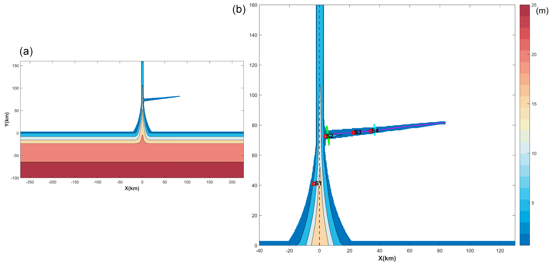
Figure 2Geometry and bathymetry of the idealized model domain: (a) for the whole domain; (b) zoom-in for the area of concern. The origin of the coordinates is in the middle of the main estuary mouth. The longitudinal sections in the main and sub-estuary are shown as dashed lines, and the cross-sections inside the sub-estuary are shown as solid colored lines. The locations of several stations are indicated.
3.2 Numerical model configuration and experiments
The Regional Ocean Modeling System (ROMS) was used in this modeling study. ROMS is a free-surface, hydrostatic, primitive-equations ocean model that uses stretched, terrain-following vertical coordinates and orthogonal curvilinear horizontal coordinates on an Arakawa C grid (Haidvogel et al., 2000). The model domain was designed as an estuary-shelf system (Fig. 2). In the coordinate system, x is in the cross-estuary direction, with rightward being positive; y is in the along-channel direction, with landward being positive; and z directs upward. The origin of the system is in the middle of the estuary mouth. The estuary is composed of a convergent part and a straight part. The geometry and bathymetry of the estuary roughly resemble those of the PRE, with the convergent part extending from the estuary mouth to the Humen Outlet (70 km in length), and the straight part from the Humen Outlet to the head of the estuary (90 km long). For the convergent part, the estuarine width B is assumed to decrease exponentially in the landward direction, as follows:
where B0 is the estuarine width at the estuary mouth (here taken as 46 km) and Lb is the width convergence length (taken as 31 km, as estimated by Zhang et al., 2021). The bathymetry of the PRE is characterized by deep channels and side shallow shoals. Following Wei et al. (2017), we roughly mimicked this feature by setting the bathymetry of the convergent part as
where L is the length of the convergent part (70 km); Hmax (20 m) and Hmin (3.0 m) are the maximum and minimum water depths at the estuary mouth; the width-averaged water depth Hm is constant (Hm = 8 m) along the estuary; and the parameter Cf is set to 4, based on the bathymetry data. In the straight part of the estuary, the bathymetry was kept the same as that of the uppermost cross-section of the convergent part.
At a distance of 75 km from the mouth of the main estuary, we added a sub-estuary on the east side, resembling the East River sub-estuary. The sub-estuary extends in a southwest–northeast direction for a distance of approximately 75 km. The width of the sub-estuary is convergent, with a width of 10 km at the confluence and decreasing to 600 m at the head, with an e-folding decreasing scale (Lb) of 26.7 km. The water depth decreases landward from 6 m at the confluence to 3.5 m at the head of the sub-estuary.
As the boundary conditions at an estuary mouth are generally unknown, we added a continental shelf to the model domain. The shelf is 100 km wide and approximately 500 km long, with the downstream part (representing the Kelvin wave propagation direction) being slightly longer than the upstream part. The water depth of the shelf is uniform in the alongshore direction and increases linearly from the coast to the offshore direction, with a slope of 1 × 10⁻⁴. The model grid has 313 × 506 cells, with a cross-channel spatial resolution of 300 m and an along-channel resolution of 500 m in the estuary. The horizontal resolution decreases on the shelf and becomes 2 km at the open-ocean boundaries. Fifteen vertical s-grid layers were specified with higher resolutions near the surface and bottom, and the coefficients θs, θb, and hc were set to 2.5, 3.0, and 5.0, respectively. In ROMS, coefficients larger than unity for θs and θb can generate higher resolutions near the surface and bottom, respectively. For details of these coefficients, Shchepetkin and McWilliams (2005) can be referred to.
We used the k−ε submodel of the generic length scale (GLS) turbulence closure scheme to calculate the vertical mixing (Umlauf and Burchard, 2003; Warner et al., 2005). The horizontal eddy viscosity and diffusivity were calculated using the Smagorinsky scheme (Smagorinsky, 1963). The bottom friction was calculated based on the log-layer assumption near the bottom, with a bottom roughness length of 1 mm. This setting results in a mean bottom drag coefficient of 0.005. The open-ocean boundary condition for the barotropic component consists of a Flather–Chapman boundary condition for the depth-averaged flow and sea surface elevation (Chapman, 1985; Flather, 1976). The open boundary conditions for the temperature, salinity, and baroclinic current are the Orlanski-type radiation conditions (Orlanski, 1976).
To investigate the impact of salt dynamics in the main estuary on salt intrusion in the sub-estuary, two numerical experiments were implemented. In both cases, the river discharge at the head of the sub-estuary was set to 200 m3 s−1, which is approximately the value during the dry season in 2021 in the East River estuary. A time series of water levels produced by a combination of 12 tidal constituents was specified at the offshore boundary. These 12 tidal constituents are M2, S2, N2, K2, K1, O1, P1, Q1, M4, MS4, Mm, and Mf. The tidal constants of these 12 constituents were obtained from the Oregon tidal database (OPTS). As the tidal amplitudes are almost doubled at the mouth of the main estuary due to the superimposition of propagating and reflected tidal waves, the amplitudes of these tidal constituents at the offshore boundary were reduced by half. Case 1 was set with a river discharge of 1500 m3 s−1 at the main estuary's head. The river discharge of 1500 m3 s−1 is representative of the total amount that empties into the PRE from different outlets in dry seasons (Gong et al., 2020), being lumped as input at the head of the PRE. The inflowing river water was prescribed to have zero salinity and a temperature of 22 ∘C, identical to the background temperature setting throughout the entire domain. The incoming salinity at the offshore boundary was specified to be 34 g kg−1. In Case 2, we set an extremely low river discharge (500 m3 s−1) at the head of the main estuary, which is realistic under the La Niña event. In this scenario, we aimed to check how the salt dynamics in the more mixed main estuary affect the salinity variation in the sub-estuary.
3.3 Analytical solutions for the salinity variation in the well-mixed sub-estuary
For the tidally averaged salinity variation along the well-mixed sub-estuary, the advection–diffusion equation can be written as
where A is the cross-sectional area, is the tidally averaged salinity in the cross-section, t is time, is tidally averaged longitudinal velocity, x is the distance along the sub-estuary, and Kx is the longitudinal dispersion coefficient. The left term in Eq. (3) indicates the local acceleration and the unsteadiness of salinity variation. The unsteadiness is controlled by the contrast between the internal and external timescales. Savenije (2012) suggested an internal timescale to quantify the sub-estuary's response timescale (TS), which is expressed as
Based on the numerical model results, by selecting X at the sub-estuary's mouth, we calculated the response timescale to be 16.22 d, which is comparable to the spring–neap tidal cycle. This indicates that the salinity in the sub-estuary can vary along with the changing tidal forcing. We thus ignored the unsteadiness term and assumed that the horizontal dispersion is constant in a tidal period and scales with the tidal current at the sub-estuary's mouth. Meanwhile, the boundary condition of tidally averaged salinity at the sub-estuary's mouth was updated in each tidal period. In this way, the calculation of tidally averaged salinity in the sub-estuary can proceed. As such, Eq. (3) becomes (Cai et al., 2015):
in which Q is the river discharge. We assume that the cross-sectional area decreases exponentially in the landward direction, , where a is the convergence length scale of the cross-sectional area. When the longitudinal dispersion coefficient Kx is assumed to be a constant along the sub-estuary, the tidally averaged salinity along the sub-estuary can be obtained as
For each tidal period, we obtained the tidally averaged salinity (S0) and the tidal current at the mouth of the sub-estuary from the numerical model results and related the horizontal dispersion (Kx) to the tidal strength at the mouth. When these data were available, the tidally averaged salinity in each tidal period was calculated for our numerical simulation period.
When Kx is assumed to vary along the estuary, the salinity variation along the sub-estuary is in another form and not presented here (Savenije, 2012), as that form of Kx is not related to the tidal strength and is unsuitable for our situation here, so this scenario is not pursued further.
3.4 Calculation of the salt and freshwater fluxes
The salt flux at a cross-section is calculated as follows:
where u is the instantaneous longitudinal velocity and S is the instantaneous salinity. The instantaneous flux was integrated and then averaged over a tidal period.
As the changes in freshwater transport by the river–tide interaction are concerned, we also calculated the freshwater flux, which is
where S0 is the ocean salinity, here is taken to be 34 g kg−1. The freshwater flux was also integrated and averaged over a tidal period.
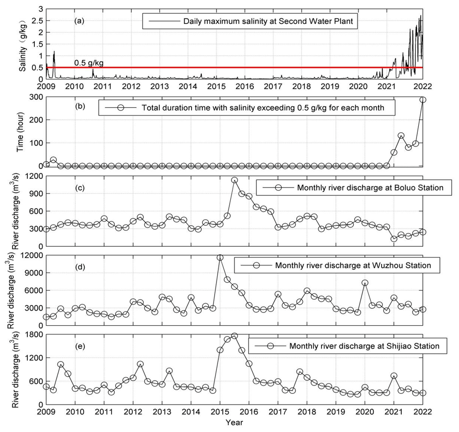
Figure 3Time series of (a) daily maximum salinity at the Second Water Plant, (b) total duration period with salinity exceeding 0.5 g kg−1 for each month, (c) monthly river discharge at Boluo Station (upstream region of the East River), (d) monthly river discharge at Wuzhou Station (upstream region of the West River), and (e) monthly river discharge at Shijiao Station (upstream region of the North River).
4.1 The characteristics of salt dynamics in the sub-estuary: based on observation data
Here we take the Second Water Plant as a representative station in the upstream region of the sub-estuary. The salinity variation at this station was checked from 2009 to 2022, as shown in Fig. 3. It indicates (Fig. 3a) that before 2021, the surface salinity was generally lower than 0.5 g kg−1 and suitable for extraction. During the winter season of 2021–2022, the salinity exceeded the drinking water criterion for a prolonged period of 280 h in January 2022 (Fig. 3b). These elevated salinities coincided with the decreased river discharge from the upstream region in the PRD, shown by the data at the hydrological stations of Boluo, Wuzhou, and Shijiao (Fig. 3c–e). Note that the river discharges in 2022 are comparable to those of 2009, but the effect on salinities is dramatically higher. The reasons behind such a difference are not clear at the moment but could be the increased water depth along the sub-estuary in 2022 by sand mining and/or the elevated water level outside the sub-estuary due to wind effects.
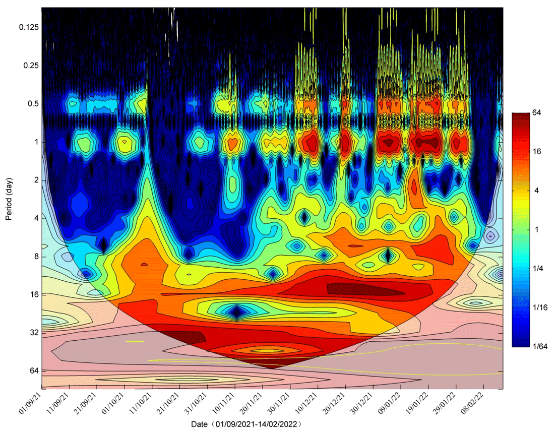
We conducted wavelet analysis for the salinity data of the Second Water Plant Station from September 2021 to February 2022, when the salt intrusion was severe. The result is shown in Fig. 4. It indicates that the power of salinity variations is concentrated in several periods: one period is in the range of 0.5 to 1 d, which is caused by tidal fluctuation; the second period lies in the range of 5–9 d, which is presumably induced by wind forcing; and the third one is in the range of 14–16 d, obviously by the fortnightly variation in spring–neap tidal cycle. The last period is within the range of 28 d, near the monthly timescale. This periodicity is probably caused by the tidal beating among the tidal constituents of M2, S2, N2, K1, and O1, as indicated by Payo-Payo et al. (2022).
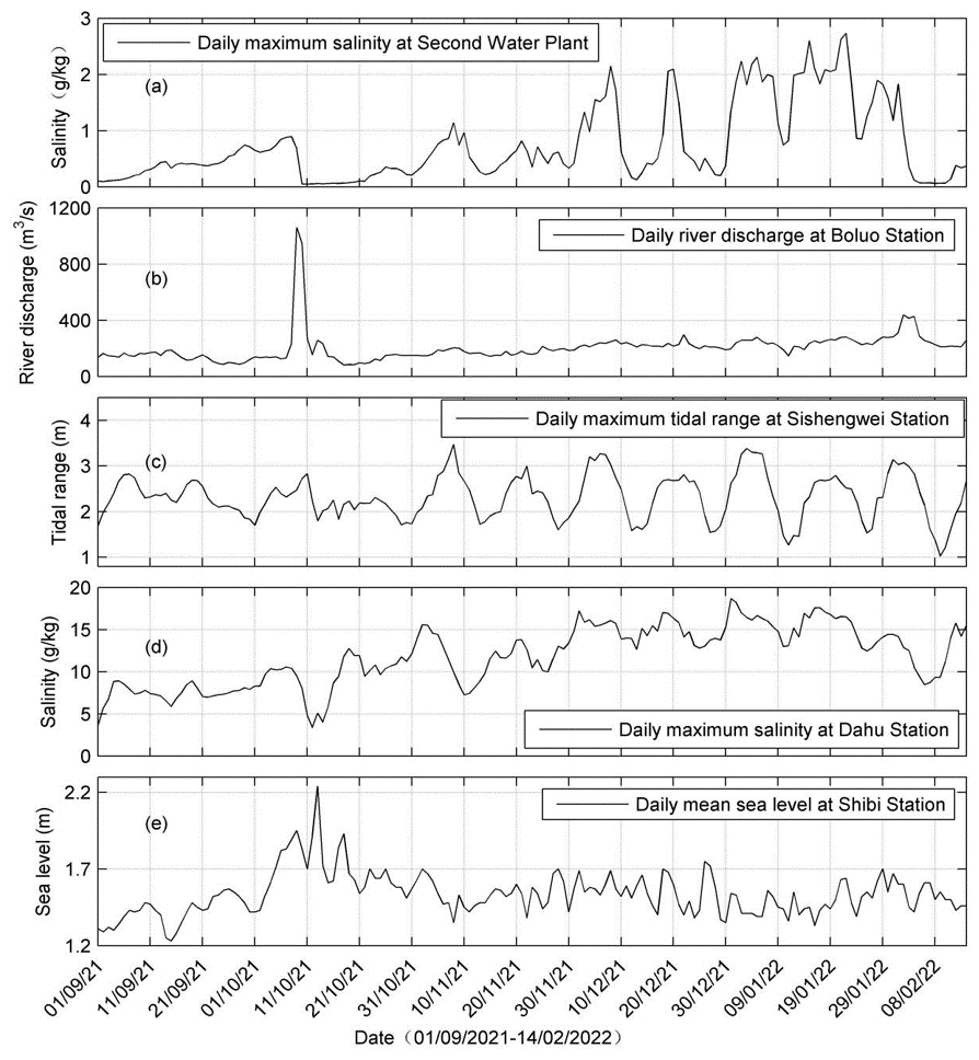
Figure 5Time series of (a) daily maximum salinity at the Second Water Plant, (b) daily river discharge at Boluo Station, (c) daily maximum tidal range at Sishengwei Station, (d) daily maximum salinity at Dahu Station, and (e) daily mean sea level at Shibi Station.
To identify the possible factors influencing the salinity variations in the sub-estuary, we present the time series data of salinity at the Second Water Plant, the river discharge at Boluo Station, the tidal range at Sishengwei Station, salinity at Dahu Station (located in the main estuary), and daily sea level at Shibi Station (located at the mouth of the main estuary) in Fig. 5. Firstly, it is evident that the variation in salinity at Dahu (Fig. 5d) shows a consistent pattern with the changes in tidal range at Sishengwei (Fig. 5c), when the river discharge is relatively low after a flash flood event, which occurred around 21 October 2021 (Fig. 5b). The highest salinity happened 2–3 d after neap tides in the transition from neap to spring tides, whereas the lowest salinity occurred in the transition from spring to neap tides and generally occurred just before the neap tides. This result indicates that the salinity and tidal range in the main estuary were almost out of phase, and there existed a time lead of the salinity to the tidal range. This pattern agrees well with what occurred in the Hudson River (Bowen and Geyer, 2003) and the Modaomen Estuary (Gong and Shen, 2011), suggesting that the PRE remained in a partially mixed state. On the other hand, the salinity of the Second Water Plant was almost in phase with the tidal range at the confluence (Fig. 5a vs. Fig. 5c). High salinities coincided with spring tides, and low salinities occurred during neap tides. It should be noted that the sea level at the PRE mouth showed a significant setup near 11 October 2021, when a large increase in river discharge was observed in the PRD due to a tropical storm (enumerated as the 17th typhoon in 2021; see the peak in Fig. 5b). This event caused a sharp decline in salinities at both Dahu and the Second Water Plant, followed by a rebound approximately 10 d later. Note that it takes about 7–8 d after the storm for the salinity to recover to its pre-storm levels in the main estuary and almost a month in the sub-estuary. The recovery time is mostly determined by the landward salt flux, as pointed out by Du and Park (2019). The landward salt flux is larger in the main estuary as it is more stratified and the estuarine circulation is more developed, which generates a larger steady shear transport. Meanwhile the width and the cross-sectional area of the main estuary are larger, favorable for the salt import from the ocean. Moreover, the station at the main estuary is located downstream of the confluence between the main estuary and the sub-estuary. After the salinity recovery at the station in the main estuary, the elevated salinity then propagates from the confluence to the upstream region of the sub-estuary, where the station at the sub-estuary is located. As the cross-section at the confluence is small, the landward salt flux is limited, further increasing the recovery time for the station at the sub-estuary.
The cross-wavelet analysis between salinity at Dahu and tidal range at Sishengwei (Fig. 6a) shows that the two variables are highly correlated in the periods of 14–16 d, indicating the effect of fortnightly spring–neap tidal variation. The arrow pointing down and right in this time band demonstrates that the change in tidal range lagged the variation in salinity.
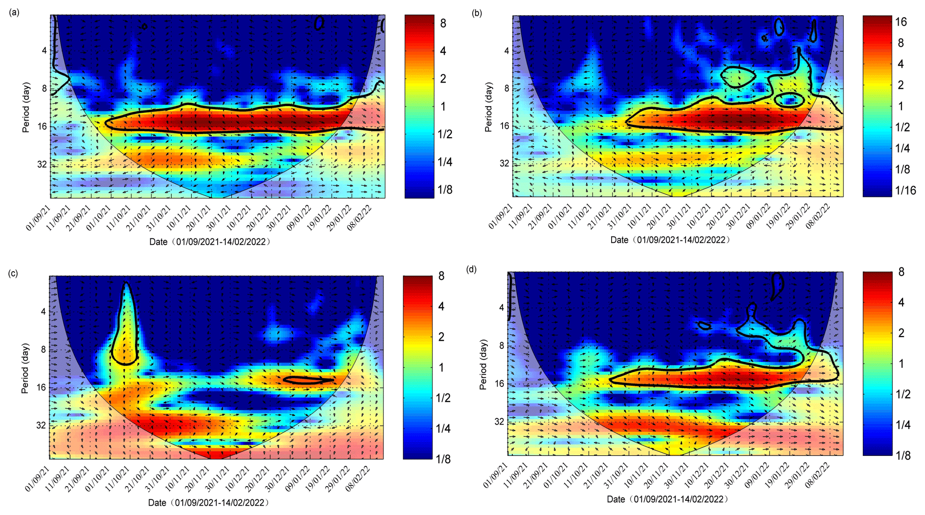
Figure 6Cross-wavelet analysis of (a) between the salinity at Dahu and the tidal range at Sishengwei, (b) between the salinity at the Second Water Plant and the tidal range at Sishengwei, (c) between the salinity at the Second Water plant and the river discharge at Boluo Station, and (d) between the salinity at the Second Water plant and that at Dahu Station.
The cross-wavelet analysis between the salinity at the Second Water Plant and the tidal range at Sishengwei Station (Fig. 6b) shows that there existed a high common power band of 14–16 d after 21 October 2021, and the phase relationship between them was in phase, indicating that high salinities occurred during spring tides and low salinities during neap tides, confirming the above results. It is also noted that before the flood event on 11 October 2021, there was no high common power between these two variables, even though the river discharge at the head of East River (Boluo Station) was lower. This lack of high common power in the time band of 14–16 d before the tropical storm event can also be noted in the cross-wavelet analysis between the salinity at Dahu and the tidal range at Sishengwei. We also noted that before the storm event, the water level at Sishengwei did not show distinct fortnightly spring–neap variations (Fig. 5c). This lack of a fortnightly cycle could be induced by the wind-induced setup/set-down and/or the river–tide interaction, in which the river flow suppresses the tidal propagation. This phenomenon is peculiar and warrants a future study, but this is beyond the scope of this study.
The cross-wavelet analysis between the salinity at the Second Water Plant and the river discharge at Boluo Station is presented in Fig. 6c. The high correlation during the storm event was obvious, whereas, after that, the common power between the salinity and river discharge was relatively low during the rebound period of the salinity at the Second Water Plant. This low correlation could be due to the fact that the river discharge did not change much and had no periodicity of 14–16 d then.
To examine the relationship between the salinities in the main estuary and at the sub-estuary, we conducted a cross-wavelet analysis between the salinity at the Second Water Plant and that at Dahu (Fig. 6d). There existed high common power between these two variables in the time band of 14–16 d, the fortnightly tidal cycle. It also shows that before 21 October 2021, the phase relationship between these two variables was approximately in quadrature, indicating that the variation in the salinity at the Second Water Plant lagged that at Dahu by 3.5–4 d. After 21 October 2021, the phase relationship between them changed to in phase when the river discharges in the PRD became very low. This is quite interesting and will be explored in the following.
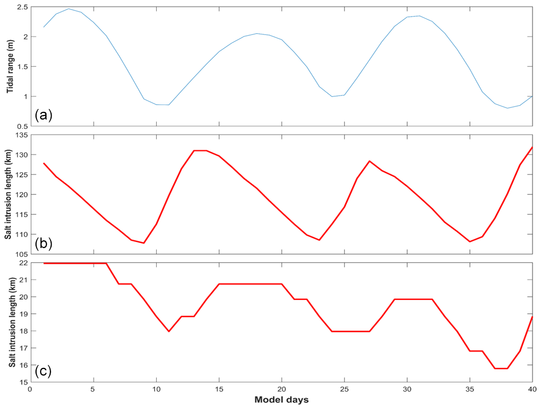
Figure 7Time series of (a) tidal range at the mouth of the main estuary, (b) salt intrusion length along the longitudinal section of the main estuary, and (c) salt intrusion length along the longitudinal section of the sub-estuary.
4.2 The salt dynamics obtained through numerical simulations
For Case 1 (base run), we intended to investigate the salt dynamics when the main estuary stays in a partially mixed state. Firstly we examine the variation in salt intrusion length along the estuary's deep channel (Fig. 2b). Here the salt intrusion length is defined as the distance of the bottom salinity isohaline of 5 g kg−1 from the estuary mouth. It shows that the tidal range at the main estuary's mouth fluctuates at fortnightly and monthly timescales. There occur two spring tides and neap tides in a month (Fig. 7a), with one spring (neap) tide being stronger than the other one, as in the perigee–apogee cycle. The salt intrusion in the main estuary fluctuates with the tidal range (Fig. 7b). The maximum salt intrusions occur just after neap tides, and the minimum salt intrusions occur 2–3 d before neap tides, consistent with the salinity change at Dahu Station shown above (Fig. 5d), and the results we have demonstrated before (Gong et al., 2018). The relationship between the salt intrusion and tidal range indicates an almost anti-phase one, suggesting that the estuary is basically in a partially mixed state. This is because, for a partially mixed estuary, the landward salt transport is maximal during neap tides by the steady shear and results in a maximum salt intrusion then. We present the tidally averaged longitudinal profile of current and salinity for representative neap and spring tides in Fig. S1 in the Supplement. The results confirm that during the neap tide, the estuary is partially mixed, whereas, during the spring tide, the estuary becomes more mixed but still in the partially mixed state.
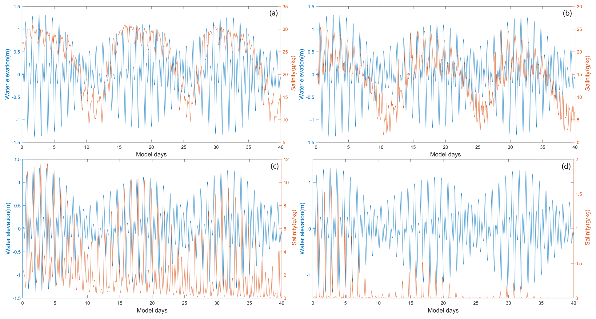
Figure 8Time series of water level at the confluence and surface salinity (a) at the S1 station in the main estuary, (b) at the S2 station (the confluence), (c) at the S3 station in the middle of the sub-estuary, and (d) at the S4 station in the upstream region of the sub-estuary.
We also checked the time series data of surface salinity and water level at a station (S1, Fig. 2b) in the main estuary, roughly corresponding to Dahu Station (Fig. 8a). It shows that the surface salinity increases from neap to spring tides, and reaches maxima before spring tides. It declines from maxima to minima from spring to neap tides, reaching minima almost at neap tides. This shows that the salinity increases faster from neap to spring than it decreases from spring to neap. This asymmetry is also noted in the variation in salt intrusion length, which increases sharply after the neap tides but decreases more gradually from the maximum to the minimum. This phenomenon has been discussed by Chen (2015); when the salt intrusion length is shorter just before the neap tide, the acceleration by the net landward salt flux is stronger, whereas when the salt intrusion length is longer, the deceleration of salt intrusion length by net seaward salt flux is relatively weaker. The change in salinity leads that in tidal range during spring tides but lags the tidal range during neap tides.
Similar to the analysis of observation data, we then investigate the salt intrusion in the sub-estuary (Fig. 7c). Though the accuracy is not high, as our model resolution in the sub-estuary is not fine enough, it clearly shows that the maximum salt intrusions occur nearly in spring tides and the minimum salt intrusions in neap tides. This means that the salt intrusion is in phase with the tidal range in the sub-estuary. We show the tidally averaged profiles of current and salinity at the sub-estuary in Fig. S2 in the Supplement. They indicate that the sub-estuary is mostly in a well-mixed state during both the neap and spring tides, though there appears some stratification near the mouth of the sub-estuary during the neap tide. The 1 g kg−1 isohaline intrudes more in spring tides than in neap tides. It should be noted that at the lower reach of the sub-estuary, the surface salinity has a local high-salinity zone (Fig. S2), consistent with the finding of Haywood et al. (1982) at the lower York River in the Chesapeake Bay, USA.
To examine the salinity variations along the sub-estuary, we selected three stations in the sub-estuary: one at the mouth (S2), one in the middle reach (S3), and the last one in the upper reach (S4). The time series of the water level at the confluence and salinities at these three stations are shown in Fig. 8b–d. The salinity at the mouth of the sub-estuary (Fig. 8b) fluctuates similarly to that in the main estuary: maximum salinities occur right after neap tides and minimum salinities just before neap tides. In the middle of the sub-estuary (Fig. 8c), the salinity variation almost keeps pace with that of the tidal range: maximum salinities occur at spring tides and minimum salinities at neap tides. At the upstream station, the salinity variation shows a similar pattern to that in the middle of the sub-estuary. This indicates that when saline water propagates upstream, it advances more landward and experiences less impedance during spring tides and vice versa when saline water propagates downstream. We explore this phenomenon in the discussion part.
4.3 The tidally averaged salt dynamics in the sub-estuary by analytical solution
We used the analytical solutions in Sect. 3.3 to explore the salt dynamics in the sub-estuary. In the sub-estuary, the exponential decaying constant of the cross-sectional area was calculated to be 50 km, and the river discharge was specified to be 200 m3 s−1.
We used the scheme of constant dispersion along the sub-estuary, and Kx was estimated as (Ralston et al., 2008):
where ch is an empirical constant of 0.0224; Ttide is the tidal period, here is set to 12.42 h; and UT is the tidal current amplitude at the sub-estuary's mouth.
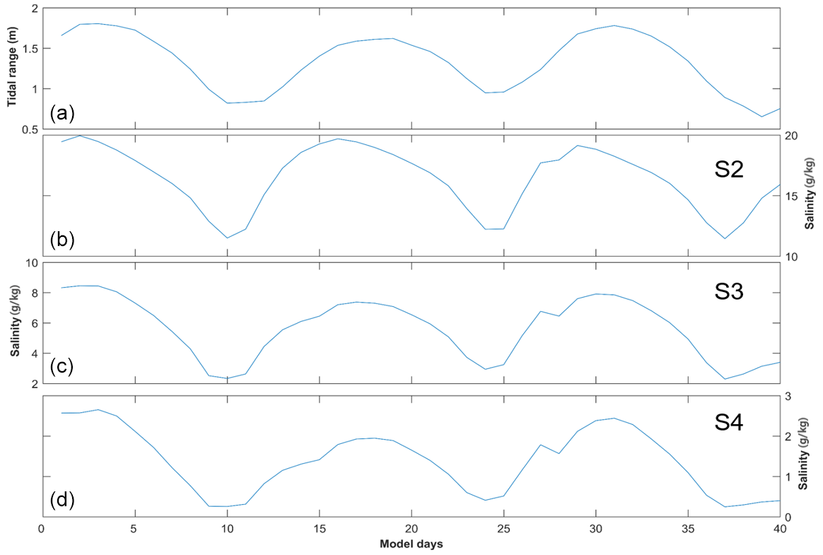
Figure 9The results of the analytical solution of salinity variations along the sub-estuary. (a) Tidal range at the mouth of the sub-estuary; (b), (c), and (d) are tidally averaged salinity variations at the S2–S4 stations.
We solved Eq. (6) for the model experiment Case 1. The results are shown in Fig. 9.
Under the 1500 m3 s−1 river discharge at the head of the main estuary, the tidal range at the sub-estuary's mouth varies between spring and neap tides, with a greater spring tide and a weaker spring tide in a month (Fig. 9a). The tidally averaged salinity at the confluence (S2 station, Fig. 9b) varies between 10 and 20 g kg−1, with the maximum salinities occurring before the spring tides and the minimum salinities before the neap tides, indicating a phase lead of salinity to the tidal range. In the middle of the sub-estuary (S3 station, Fig. 9c), the salinity fluctuates between 2 and 10 g kg−1, and there exists a slight phase lead of salinity to that of the tidal range. In the upstream region of the sub-estuary (S4 station, Fig. 9d), the salinity fluctuates between 0 and 3 g kg−1, and the salinity variation becomes almost in phase with that of the tidal range at the confluence. Compared to the numerical simulation results, the analytical solution reproduces the trend of the phase relationship between the salinity and tidal range along the sub-estuary: the phase of the salinity variation leads that of the tidal range at the sub-estuary's mouth and becomes more in phase with that of the tidal range in the middle and upstream region of the sub-estuary. Meanwhile, the fluctuation magnitude in the middle of the sub-estuary is well reproduced. However, the fluctuation range in the upstream region of the sub-estuary is overestimated, showing the weakness of assuming a uniform horizontal dispersion along the sub-estuary.
5.1 The physics behind the change in phase relationship between the salinity and tidal range along the sub-estuary
The numerical results and analytical solutions both indicate that near the sub-estuary's mouth, the salinity fluctuation leads that of the tidal range and that in the middle and upstream region of the sub-estuary, the salinity variation becomes more in phase with that of the tidal range. The analytical solution shows that the changes in the phase relationship between these two variables are mostly caused by the change in horizontal dispersion; that is, the larger dispersions during spring tides cause increased landward salt transport, resulting in elevated salinity in the middle and upstream regions of the sub-estuary. The results of numerical simulation are a combination of many interwoven processes and a little harder to interpret. To unravel the physics in the numerical simulation, we examine the salt transport in the lower reach at a cross-section near the sub-estuary mouth and freshwater transport in the upstream cross-section of the sub-estuary (shown in Fig. 2b).
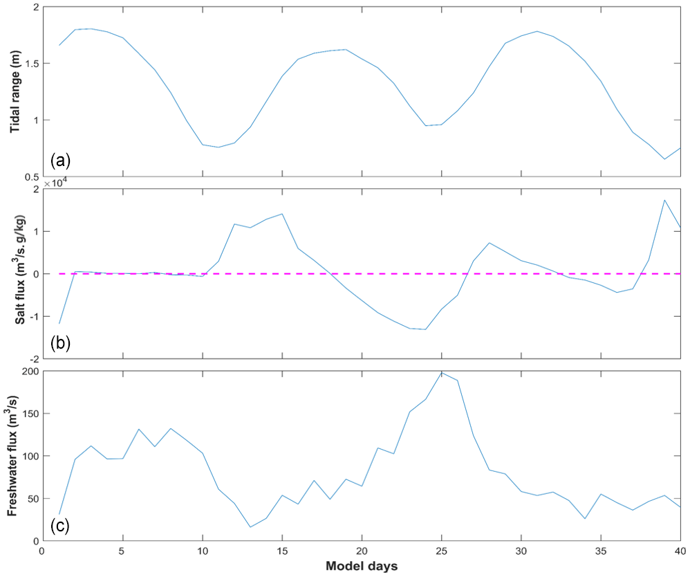
Figure 10Time series of (a) tidal range at the mouth of the sub-estuary, (b) salt flux at the cross-section near the mouth of the sub-estuary, and (c) freshwater flux at the cross-section in the upstream region of the sub-estuary.
The results are shown in Fig. 10. From Fig. 10b, the tidally averaged salt flux near the sub-estuary's mouth is generally landward during the periods from neap tides to spring tides and seaward from spring tides to neap tides. The change in salt flux leads that of the tidal range, consistent with the phase relationship between salinity and tidal range near the sub-estuary's mouth (Fig. 8b). As the sub-estuary is well-mixed during the simulation period, the landward salt transport is mostly induced by the tidal oscillatory transport. The tidally averaged freshwater flux in the upstream region of the sub-estuary is seaward and shows a pattern that larger freshwater fluxes occur during neap tides and smaller freshwater fluxes during spring tides (Fig. 10c). This pattern has been well studied by Buschman et al. (2009) in the tidally averaged momentum dynamics. They showed that the primary tidally averaged momentum balance is between the water level gradient and bottom friction. During spring tides, the tidally averaged bottom friction is larger and the tidally averaged water slope is greater, meaning that more freshwater is being detained upstream to elevate the water level there. During neap tides, the detained freshwater in the upstream region is released downstream and results in increased freshwater fluxes. In this way, the saline water from the sub-estuary's mouth experiences less impedance and dilution during spring tides and thus advances more landward, resulting in an enhanced salt intrusion during spring tides, and vice versa during neap tides. The above results indicate that the more in-phase relationship between the salinity and tidal range in the middle and upstream region of the sub-estuary is mostly generated by the fortnightly variation in the tidal strength and the associated variations in horizontal dispersion and freshwater flux by the river–tide interaction. The larger the dispersion, the more salt is pumped into the upstream region. The stronger the tidal strength, the more freshwater is detained upstream and the less impedance there is to salt intrusion.
From the above results, it is seen that the salinity dynamics in the sub-estuary show a pattern that is more influenced by the main estuary in the lower reach and becomes more controlled by internal tidal processes in the middle and upstream regions of the sub-estuary.
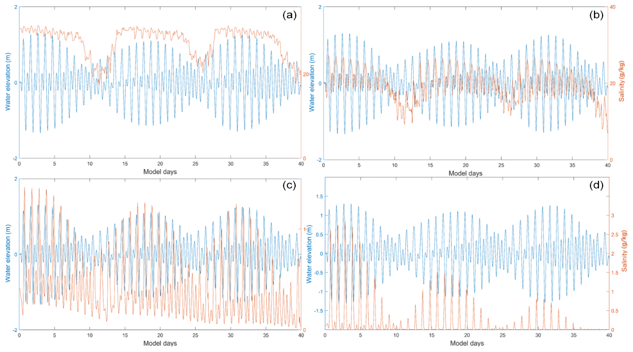
Figure 11Time series of water level at the confluence and surface salinity under the extremely low river discharge in the main estuary at stations (a) S1, (b) S2, (c) S3, and (d) S4.
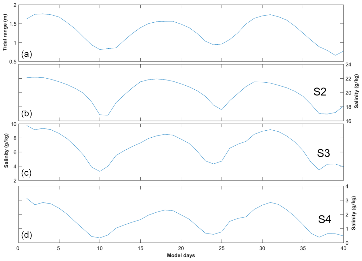
Figure 12The results of the analytical solution of salinity variations along the sub-estuary under extremely dry conditions. (a) Tidal range at the mouth of the sub-estuary; (b), (c), and (d) are tidally averaged salinity variations at the S2–S4 stations.
5.2 How do the salt dynamics in the main estuary affect that in the sub-estuary?
To further study how the changes in salinity dynamics in the main estuary affect the salinity variation in the sub-estuary, we set up another experiment. In the model scenario of Case 2, we set an extremely low river discharge (500 m3 s−1) at the head of the main estuary, and the results are shown in Fig. 11. Simultaneously, the analytical solutions for the scenario of Case 2 are presented in Fig. 12.
With decreased river discharge from the head of the main estuary, the salt intrusion front is shifted more landward. The S1 station is now located in the polyhaline region with a mean salinity of approximately 26 g kg−1 (Fig. 11a). The minimum salinities coincide more with neap tides but the maximum salinities occur around spring tides. The asymmetry between salinity rise and fall is decreased, with salinities jumping quickly after neap tides, staying elevated around spring tides, and dropping quickly just before neap tides. For the intratidal variation, it can be seen that during a tidal cycle, the salinity fluctuation is reduced when compared to Case 1 (Fig. 11a vs. Fig. 8a), which is mostly due to the fact that with the reduced river discharge, the salinity gradient in the polyhaline reach of the main estuary is decreased.
For the S2 station (at the confluence, Figs. 11b and 12b), it is now located in the mesohaline region, with the salinity ranging from 5 to 26 g kg−1. The highest and lowest salinities are both increased when compared to Case 1, with a reduced magnitude of salinity change in a tidal cycle. The salinity variation pattern remains similar to that in Case 1, with minimum salinities occurring just before neap tides and maximum salinities after neap tides but closer to spring tides. The asymmetry of a quick increase from neap to spring but gradual decrease afterwards is still clear.
When entering into the sub-estuary, the salinity variation at S3 in the middle of the sub-estuary shows a more in-phase relationship between salinity and tidal range (Figs. 11c and 12c). The maximum salinities occur closer to spring tides, whereas the minimum salinities still occur just before neap tides. In the upstream region of the sub-estuary (Figs. 11d and 12d), the phase relationship between salinity and tidal range is also an in-phase one. Combined with the situation at the S1 station, it indicates that the variations in salinity at stations S4 and S1 are more synchronous. This largely explains the observed phenomenon that under stronger drought conditions, the salinity variations at the Second Water Plant kept pace with those at Dahu Station (Sect. 3.1).
5.3 Limitations and implications of this study
In this study, we focus on the phase relationship between the variations in salinity and tidal range, both in a sub-estuary and the main estuary. The salinity variations along the sub-estuary are revealed to be associated with the salinity dynamics in the main estuary, linked by the salinity variations at the confluence between the main estuary and the sub-estuary. In a spring–neap tidal cycle, even when the salinity at the confluence is a little lower during the spring tide than that during the neap tide, the higher horizontal dispersion and decreased freshwater release at the head of the sub-estuary during the spring tide can pump more saline water from the confluence into the middle and upstream regions of the sub-estuary and cause the salinities there to be higher than during the neap tide. In this way, the salinity variations at areas farther away from the confluence become more synchronous with the tidal range.
However, this study did not consider the effect of winds and waves, shown to be important in previous studies such as Gong et al. (2018). The variations in salinity in the period of 5–8 d should be related to the wind effects and await future exploration. The effect of sea level change outside the main estuary was also not examined in detail, though it can be intrinsically linked to the effect of winds and waves. Finally, we did not explore a full parameter space of river discharge, tidal range, and bathymetry situations and thus cannot give a synthesis of the sub-estuary salt intrusion dynamics at this time.
Despite all these limitations, this study has implications for studying salt intrusion dynamics in sub-estuaries, which are influenced by both the hydrodynamics inside the sub-estuary and the salt dynamics in the main estuaries. It is also of importance for providing a scientific basis for salt intrusion mitigation in the region. For example, salt intrusion in the sub-estuary is not only impacted by the river discharge from the head of the sub-estuary itself but also largely affected by the salt dynamics in the main estuary. In this respect, apart from releasing more freshwater from the upstream region into the sub-estuary, measures to control the salinity variations at the confluence between the main estuary and the sub-estuary also need to be taken into consideration. This may involve implementing engineering solutions such as the construction of barriers or gates to regulate the inflow of saltwater from the main estuary into the sub-estuary. Additionally, the management of water withdrawals and releases in the sub-estuary and main estuary needs to be optimized by considering the estuarine system as a whole. Overall, a comprehensive and coordinated approach is necessary to effectively mitigate salt intrusion in sub-estuaries.
From 2021 to 2022, under the influence of an extended La Niña event, the Pearl River Delta region in China experienced a prolonged extreme drought condition, and the sub-estuary (East River estuary) also suffered greatly from the enhanced salt intrusion. To identify the characteristics of the salt intrusion in the sub-estuary and to explore the underlying physics in controlling the spatiotemporal variations in the salt intrusion, we collected observation data and conducted numerical simulations for idealized estuarine bathymetry and used analytical solutions for the tidally averaged salinity variations in the sub-estuary. The observation data showed that the salinity variation in the main estuary usually led that of the tidal range, and the asymmetry between salinity rise and fall on a fortnightly timescale was prominent. However, in the upstream region of the sub-estuary, the salinity variation was in phase with that of the tidal range, and the salinity rise and fall were more symmetrical. The idealized model simulations and the analytical solution both reproduced these phenomena.
We note that under drought conditions, the river–tide interaction played a role in the in-phase relationship between the salinity and tidal range in the upstream region of the sub-estuary. The salinity variation in the middle and upstream regions of the sub-estuary can keep pace with that of the tidal range. The analytical results show that the horizontal dispersion scaling with tidal strength can largely reproduce the changes in phase relationship between salinity and tidal range in the sub-estuary. We conclude that both the changes in horizontal dispersion and the river–tide interaction in modulating the freshwater release are responsible for the in-phase relationship between the salinity and tidal range in the middle and upstream regions of the sub-estuary.
This study is of help in the investigation of salt dynamics in sub-estuaries connected to main estuaries and of implications for mitigating salt intrusion problems in the regions suffering from enhanced salt intrusion as a result of climate change and human interventions.
The observation data can be downloaded from the website http://www.pearlwater.gov.cn/ (Pearl River Water Resources Commission of the Ministry of Water Resources, 2024). The numerical data are available upon request to the corresponding author.
We present the longitudinal profiles of tidally averaged current and salinity along the channels in the main estuary and the sub-estuary during typical spring and neap tides. Figure S1 is for the dry conditions with 1500 m3 s−1 at the head of the main estuary and Fig. S2 for the extremely dry conditions with 500 m3 s−1 released at the head of the main estuary. The supplement related to this article is available online at: https://doi.org/10.5194/os-20-181-2024-supplement.
ZL: data collection, wavelet analysis, writing (original draft), and writing (review and editing). GZ: numerical modeling, and writing (review and editing). HZ: writing (review and editing) and funding acquisition. WG: conceptualization, methodology, writing (review and editing), and funding acquisition.
The contact author has declared that none of the authors has any competing interests.
Publisher's note: Copernicus Publications remains neutral with regard to jurisdictional claims made in the text, published maps, institutional affiliations, or any other geographical representation in this paper. While Copernicus Publications makes every effort to include appropriate place names, the final responsibility lies with the authors.
This article is part of the special issue “Oceanography at coastal scales: modelling, coupling, observations, and applications”. It is not associated with a conference.
Hubert H. G. Savenije at the Delft University of Technology and another anonymous reviewer are greatly appreciated for their constructive comments and suggestions to improve this paper. We would also like to thank the editor John M. Huthnance for his great insights into the scientific issues raised in this paper.
This research has been supported by the National Natural Science Foundation of China (grant nos. 42276169 and 42306015) and the Technology Innovation Program from Water Resources of Guangdong Province (2023-01).
This paper was edited by John M. Huthnance and reviewed by Hubert H. G. Savenije and one anonymous referee.
Bowden, K. F.: Horizontal mixing in the sea due to a shearing current, J. Fluid Mech., 21, 83–95, https://doi.org/10.1007/BF00167972, 1965.
Bowen, M. and Geyer, W. R.: Salt transport and the time-dependent salt balance of a partially stratified estuary, J. Geophys. Res., 108, 3185, https://doi.org/10.1029/2001JC001231, 2003.
Buschman, F. A., Hoitink, A. J. F., and Vegt., M. V. D.: Subtidal water level variation controlled by river flow and tides, Water. Resour. Res., 45, W10420, https://doi.org/10.1029/2009WR008167, 2009.
Cai, H., Savenije, H. H. G., Zuo, S., Jiang, C., and Chua, V. P.: A predictive model for salt intrusion in estuaries applied to the Yangtze estuary, J. Hydrol., 529, 1336–1349, https://doi.org/10.1016/j.jhydrol.2015.08.050, 2015.
Chapman, D. C.: Numerical Treatment of Cross-Shelf Open Boundaries in a Barotropic Coastal Ocean Model, J. Phys. Oceanogr., 15, 1060–1075, https://doi.org/10.1175/1520-0485(1985)015<1060:NTOCSO>2.0.CO;2, 1985.
Chen S.-N.: Asymmetric Estuarine Responses to Changes in River Forcing: A Consequence of Nonlinear Salt Flux, J. Phys. Oceanogr., 45, 2836–2847, https://doi.org/10.1175/JPO-D-15-0085.1, 2015.
Dong, L., Su, J., Wong, L., Cao, Z., and Chen, J.-C.: Seasonal variation and dynamics of the Pearl River plume, Cont. Shelf Res., 24, 1761–1777, https://doi.org/10.1016/j.csr.2004.06.006, 2004.
Du, J. and Park, K.: Estuarine salinity recovery from an extreme precipitation event: Hurricane Harvey in Galveston Bay, Sci. Total Environ., 670, 1049–1059, https://doi.org/10.1016/j.scitotenv.2019.03.265, 2019.
Flather, R. A.: A tidal model of the northwest European continental shelf, Mem. Soc. R. Sci. Liege,, 10, 141–164, 1976.
Gong, W. and Shen, J.: The response of salt intrusion to changes in river discharge and tidal mixing during the dry season in the Modaomen Estuary, China, Cont. Shelf Res., 31, 769–788, https://doi.org/10.1016/j.csr.2011.01.011, 2011.
Gong, W., Lin, Z., Chen, Y., Chen, Z., and Zhang, H.: Effect of winds and waves on salt intrusion in the Pearl River estuary, Ocean Sci., 14, 139–159, https://doi.org/10.5194/os-14-139-2018, 2018.
Gong, W., Chen, L., Zhang, H., Yuan, L., and Chen, Z.: Plume Dynamics of a Lateral River Tributary Influenced by River Discharge From the Estuary Head, J. Geophys. Res.-Oceans., 125, e2019JC015580, https://doi.org/10.1029/2019JC015580, 2020.
Gong, W., Lin, Z., Zhang, and H., Lin H.: The response of salt intrusion to changes in river discharge, tidal range, and winds, based on wavelet analysis in the Modaomen estuary, China, Ocean Coast Manage., 219, 106060, https://doi.org/10.1016/j.ocecoaman.2022.106060, 2022.
Haidvogel, D. B., Arango, H. G., Hedstrom, K., Beckmann, A,.Malanotte-Rizzoli, B., Shchepetkin, and A., F.: Model evaluation experiments in the North Atlantic Basin: Simulations in nonlinear terrain-following coordinates, Dynam. Atmos. Oceans, 32, 239–281, https://doi.org/10.1016/S0377-0265(00)00049-X, 2000.
Haywood, D., Welch, C. S., and Hass, L. W.: York River destratification: an estuary-sub-estuary interaction, Science, 216, 1413–1414, https://doi.org/10.1126/science.216.4553.1413, 1982.
Hong, B., Liu, Z., Shen, J., Wu, H., Gong, W., Xu, H., and Wang, D.: Potential physical impacts of sea-level rise on the Pearl River Estuary, China, J. Marine Syst., 201, 103245, https://doi.org/10.1016/j.jmarsys.2019.103245, 2020.
Hu, J., Li, S., and Geng, B.: Modeling the mass flux budgets of water and suspended sediments for the river network and estuary in the Pearl River Delta, China, J. Marine Syst., 88, 252–266, https://doi.org/10.1016/j.jmarsys.2011.05.002, 2011.
Jia, L., Luo, Z., Yang, Q., Ou, S., and Lei, Y.: The impact of massive sand mining on the morphology and tidal dynamics in the downstream of East River and the East River Delta, Acta Geographica Sinica, 09, 985–994, 2006 (in Chinese).
Liu, B., Yan, S., Chen, X., Lian, Y., and Xin, Y.: Wavelet analysis of the dynamic characteristics of saltwater intrusion – A case study in the Pearl River Estuary of China, Ocean Coast Manage., 95, 81–92, https://doi.org/10.1016/j.ocecoaman.2014.03.027, 2014.
MacCready, P. and Geyer, W. R.: Advances in estuarine physics, Annu. Rev. Mar. Sci., 2, 35–58, https://doi.org/10.1146/annurev-marine-120308-081015, 2010.
Mao, Q., Shi, P., Yin, K., Gan, J., and Qi, Y.: Tides and tidal currents in the Pearl River Estuary, Cont. Shelf Res., 24, 1797–1808, https://doi.org/10.1016/j.csr.2004.06.008, 2004.
Okubo, A.: Effect of shoreline irregularities on streamwise dispersion in estuaries and other embayments, Neth. J. Sea Res., 6, 213–224, https://doi.org/10.1016/0077-7579(73)90014-8, 1973.
Orlanski, I.: A simple boundary condition for unbounded hyperbolic flows, J. Comput. Phys., 21, 251–269, https://doi.org/10.1016/0021-9991(76)90023-1, 1976.
Payo-Payo, M., Bricheno, L. M., Dijkstra, Y. M., Cheng, W., Gong, W., and Amoudry, L. O.: Multiscale temporal response of salt intrusion to transient river and ocean forcing, J. Geophys. Res.-Oceans., 127, e2021JC017523, https://doi.org/10.1029/2021JC017523, 2022.
Pearl River Water Resources Commission of the Ministry of Water Resources: http://www.pearlwater.gov.cn/, last access: 15 February 2024.
Ralston, D. K. and Geyer, W. R.: Response to channel deepening of the salinity intrusion, estuarine circulation, and stratification in an urbanized estuary, J. Geophys. Res.-Oceans., 124, 4784–4802, https://doi.org/10.1029/2019JC015006, 2019.
Ralston, D. K., Geyer, W. R., and Lerczak, J. A.: Subtidal Salinity and Velocity in the Hudson River Estuary: Observations and Modeling, J. Phys. Oceanogr., 38, 753–770, https://doi.org/10.1175/2007JPO3808.1, 2008.
Ralston, D. K., Geyer, W. R., and Lerczak, J. A.: Structure, variability, and salt flux in a strongly forced salt wedge estuary, J. Geophys. Res., 115, C06005, https://doi.org/10.1029/2009JC005806, 2010.
Savenije, H. H. G.: Salinity and tides in alluvial estuaries, 2nd Edn., http://www.salinityandtides.com (last access: 15 February 2024), 2012.
Shchepetkin, A. F. and McWilliams, J. C.: The regional ocean modeling system (ROMS): A split-explicit, free-surface, topography-following coordinates oceanic model, Ocean Model., 9, 347–404, https://doi.org/10.1016/j.ocemod.2004.08.002, 2005.
Simpson, J. H., Brown, J., Matthews, J. P., and Allen, G.: Tidal straining, density currents, and stirring in the control of estuarine stratification, Estuaries, 13, 125–132, 1990.
Smagorinsky, J.: General Circulation Experiments with the Primitive Equation, Part 1, the Basic Experiment, Mon. Weather Rev., 91, 99–164, https://doi.org/10.1175/1520-0493(1963)091<0099:GCEWTP>2.3.CO;2, 1963.
Spinoni, J., Naumann, G., Carrao, H., Barbosa, P., and Vogt, J.: World drought frequency, duration, and severity for 1951–2010, Int. J. Climatol., 34, 2792–2804, https://doi.org/10.1002/joc.3875, 2014.
Stommel, H. and Farmer, H. G.: On the nature of estuarine circulation: part I, chapters 3 and 4, Woods Hole Oceanographic Institution, https://doi.org/10.1575/1912/2032, 1952.
Umlauf, L. and Burchard, H.: A generic length-scale equation for geophysical turbulence models, J. Mar. Res., 61, 235–365, https://doi.org/10.1357/002224003322005087, 2003.
Uncles, R. J. and Stephens, J. A.: Turbidity and sediment transport in a muddy sub-estuary, Estuar. Coast. Shelf S., 87, 213–224, https://doi.org/10.1016/j.ecss.2009.03.041, 2010.
Warner, J. C., Sherwood, C. R., Arango, H. G., and Signell, R. P., and Butman, B.: Performance of four turbulence closure models implemented using a generic length scale method, Ocean Model., 8, 81–113, 2005.
Wei, X., Kumar, M., and Schuttelaars, H. M.: Three-dimensional salt dynamics in well-mixed estuaries: influence of estuarine convergence, Coriolis, and bathymetry, J. Phys. Oceanogr., 47, 1843–1872, https://doi.org/10.1016/j.ocemod.2003.12.003, 2017.
Wong, L. A., Chen, J. C., Xue, H., Dong, L. X., Su, J. L., and Heinke, G.: A model study of the circulation in the Pearl River Estuary (PRE) and its adjacent coastal waters: 1. Simulations and comparison with observations, J. Geophys. Res., 108, https://doi.org/10.1029/2002jc001451, 2003.
Wu, Z. Y., Saito, Y., Zhao, D. N., Zhou, J. Q., Cao, Z. Y., and Li, S. J.: Impact of human activities on subaqueous topographic change in Lingding Bay of the Pearl River estuary, China, during 1955–2013, Sci. Rep-UK, 6, 37742, https://doi.org/10.1038/srep37742, 2016.
Yellen, B., Woodruff, J. D., Ralston, D. K., MacDonald, D. G., and Jones. D. S.: Salt wedge dynamics lead to enhanced sediment trapping within side embayments in high-energy estuaries, J. Geophys. Res.-Oceans., 122, 2226–2242, https://doi.org/10.1002/2016JC012595, 2017.
Zhang, P., Yang, Q., Wang, H., Cai, H., Liu, F., Zhao, T., and Jia, L.: Stepwise alterations in tidal hydrodynamics in a highly human-modified estuary: The roles of channel deepening and narrowing, J. Hydrol., 597, 126153, https://doi.org/10.1016/j.jhydrol.2021.126153, 2021.
Zimmerman, J. T. F.: The tidal whirlpool: A review of horizontal dispersion by tidal and residual currents, Neth. J. Sea Res., 20, 133–154, https://doi.org/10.1016/0077-7579(86)90037-2, 1986.