Ensemble analysis and forecast of ecosystem indicators in the North Atlantic using ocean colour observations and prior statistics from a stochastic NEMO–PISCES simulator

This study is anchored in the H2020 SEAMLESS project (https://www.seamlessproject.org, last access: 29 January 2024), which aims to develop ensemble assimilation methods to be implemented in Copernicus Marine Service monitoring and forecasting systems, in order to operationally estimate a set of targeted ecosystem indicators in various regions, including uncertainty estimates. In this paper, a simplified approach is introduced to perform a 4D (space–time) ensemble analysis describing the evolution of the ocean ecosystem. An example application is provided, which covers a limited time period in a limited subregion of the North Atlantic (between 31 and 21^∘ W, between 44 and 50.5^∘ N, between 15 March and 15 June 2019, at a $\mathrm{1}/\mathrm{4}$^∘ and a 1 d resolution). The ensemble analysis is based on prior ensemble statistics from a stochastic NEMO (Nucleus for European Modelling of the Ocean)–PISCES simulator. Ocean colour observations are used as constraints to condition the 4D prior probability distribution.

As compared to classic data assimilation, the simplification comes from the decoupling between the forward simulation using the complex modelling system and the update of the 4D ensemble to account for the observation constraint. The shortcomings and possible advantages of this approach for biogeochemical applications are discussed in the paper. The results show that it is possible to produce a multivariate ensemble analysis continuous in time and consistent with the observations. Furthermore, we study how the method can be used to extrapolate analyses calculated from past observations into the future. The resulting 4D ensemble statistical forecast is shown to contain valuable information about the evolution of the ecosystem for a few days after the last observation. However, as a result of the short decorrelation timescale in the prior ensemble, the spread of the ensemble forecast increases quickly with time. Throughout the paper, a special emphasis is given to discussing the statistical reliability of the solution.

Two different methods have been applied to perform this 4D statistical analysis and forecast: the analysis step of the ensemble transform Kalman filter (with domain localization) and a Monte Carlo Markov chain (MCMC) sampler (with covariance localization), both enhanced by the application of anamorphosis to the original variables. Despite being very different, the two algorithms produce very similar results, thus providing support to each other's estimates. As shown in the paper, the decoupling of the statistical analysis from the dynamical model allows us to restrict the analysis to a few selected variables and, at the same time, to produce estimates of additional ecological indicators (in our example: phenology, trophic efficiency, downward flux of particulate organic matter). This approach can easily be appended to existing operational systems to focus on dedicated users' requirements, at a small additional cost, as long as a reliable prior ensemble simulation is available. It can also serve as a baseline to compare with the dynamical ensemble forecast and as a possible substitute whenever useful.

1 Introduction

Combining numerical models with observational data to reconstruct the past evolution of ocean biogeochemistry and to predict its future evolution has been a major objective of operational ocean forecasting centres for many years, motivated both by the marine user's needs and by advances in scientific knowledge of the ocean functioning (Gehlen et al., 2015).

In order to support decision-making or reliable scientific assessment, the marine ecosystem and biogeochemical parameters to be estimated (e.g. phenology, trophic efficiency, downward carbon flux) must be supplemented with uncertainties to quantify the robustness of the information produced and quantify the likelihood of estimates (Modi et al., 2022). This motivates the development of systems capable of producing information which is probabilistic in nature. This study is anchored in the H2020 SEAMLESS project, which aims to develop ensemble assimilation methods to be implemented in Copernicus Marine Service monitoring and forecasting systems, in order to operationally estimate a set of targeted ecosystem indicators in the different regions covered, including uncertainty estimates.

Despite their cost with high-dimensional systems, ensemble methods based on Monte Carlo simulations are well suited to generate samples of the probability distributions of the quantities of interest, as is already implemented today by some teams of the OceanPredict programme (Fennel et al., 2019). The standard approach relies on implementations of sequential ensemble data assimilation methods that typically consist of variants of the ensemble Kalman filter (Evensen, 2003). The data assimilation algorithms typically perform ensemble analysis and predictions in sequence to integrate observational information such as satellite ocean colour and ARGO BGC profile data into coupled 3D physical–biogeochemical models (Gutknecht et al., 2022).

In these ensemble data assimilation systems, the most expensive numerical component is the coupled physical–biogeochemical model that is used to perform the ensemble simulations because it is usually sought to run at high horizontal resolution and because a few dozens of members are usually necessary to obtain ensemble statistics that are accurate enough for data assimilation. The aim of this paper is to demonstrate that it is possible to make an additional use of these expensive model data, obtained from a prior ensemble model simulation (not yet conditioned on observations), to produce a statistically driven analysis and forecast for selected key model variables. A secondary aim of this paper is to illustrate the extension of the approach to estimate ecological indicators diagnosed from model state variables.

For instance, using the statistics of the ensemble, it is not difficult, at least in principle, to obtain a 4D multivariate statistical analysis based on all available observations over a given time period (possibly quite long, typically between 1 month and 1 year, maybe longer). This just corresponds to applying any standard Bayesian observational update algorithm in four dimensions (4D) to condition the prior ensemble on the observations and thus produce the corresponding 4D ensemble statistical analysis. In practice, this can for instance be achieved by a direct application of just one analysis step of the ensemble optimal interpolation (EnOI) algorithm (e.g. Evensen, 2003; Oke et al., 2010), for a 4D estimation vector (thus embedding the time evolution of the system, as in Mattern and Edwards, 2023, but over an extended time window). However, it is important to emphasize that, unlike EnOI, we do not use historical data to prescribe the prior statistics but an ensemble simulation that is specifically performed for the requested time period. This is necessary if we want to avoid assuming stationarity of the statistics.

Moreover, if the prior ensemble extends into the future, the result of the observational update can include an ensemble statistical forecast of the state of the system based on past observations. This forecast only relies on the statistical dependence between past and future as described by the prior ensemble, and as interpreted by the observational update algorithm. Such a 4D statistical analysis and forecast can be seen as an additional byproduct of the system, which could be obtained at negligible cost (as compared to the ensemble simulations).

Furthermore, the decoupling between model simulations and inverse methods substantially reduces the complexity of the numerical apparatus, which becomes more easily manageable and more flexible. Without the need to initialize the dynamical model, the ensemble analysis and forecast do not need to include the full state vector but can concentrate on a few variables or diagnostics, possibly for a specific subregion, where the result is most needed. As illustrated in this paper, the possibility of reducing the dimension of the inverse problem opens new prospects in terms of inverse method, which can be more sophisticated, and thus more able to deal accurately with complex prior ensemble statistics, nonlinear observation operators and non-Gaussian observation errors. For these reasons, there are certainly practical situations in which it would be interesting to append such a 4D statistical analysis and forecast to existing ensemble data assimilation systems. They may serve as a baseline to compare with the dynamical ensemble forecast and as a possible substitute whenever useful.

The obvious shortcoming of this approach is that the complex nonlinear dynamical model is no longer directly used to constrain the solution but only indirectly through the statistics of the prior ensemble. Moreover, if the prior ensemble has been run a long time from a realistic initial condition, the prior ensemble spread may be substantially larger than in classic data assimilation systems, with prior members possibly further away from the observations. In this respect, the approach is clearly suboptimal as compared to existing ensemble 4D analysis methods like the 4D Ensemble Variational (4DEnVar; Buehner et al., 2013) and the two-step ensemble smoother (see Van Leeuwen et al., 1996; Cosme et al., 2012, for a review of ensemble smoothers), which were developed in the framework of the well-known 4DVar and Kalman filter methods.

However, the approach proposed here also brings important advantages explained above (use of past and future observations, statistical forecast capability, simplification of the inverse problem), especially if the model is very sensitive to small imbalances in the initial condition and if it is difficult to produce an accurate ensemble analysis for all influential model state variables (e.g. by lack of sufficient observations), as is often the case with ocean biogeochemical models. In such cases, the suboptimality of the approach (in the use of the dynamical constraint) can easily be counterbalanced by a better robustness and reliability.

The objective of this paper is to assess the strengths and weaknesses of this strategy by producing a 4D analysis and forecast of ecosystem variables and indicators for a small subregion ($\mathrm{10}{}^{\circ }\times \mathrm{6.5}{}^{\circ }$) in the North Atlantic. The prior 40-member ensemble is produced with a global $\mathrm{1}/\mathrm{4}{}^{\circ }$ resolution NEMO(Nucleus for European Modelling of the Ocean)–PISCES model configuration (prepared by Mercator Ocean International, later referred to as MOI), with stochastic parameterization of uncertainties. Observations are the L3 product of chlorophyll data from ocean colour satellites. The results are illustrated for observed and non-observed variables, including ecosystem indicators, which are not model state variables. Probabilistic scores are used to evaluate the reliability and accuracy of the ensemble forecasts of chlorophyll concentration.

In addition, we show that the proposed strategy is compliant with a variety of observational update schemes similar to those in use today in operational systems. Two observational update algorithms are considered in the present paper to condition the prior ensemble on the observations. The first one is the analysis step of the ensemble transform Kalman filter (ETKF; Bishop et al., 2001) with domain localization (e.g. Janjic et al., 2011), using an implementation framework inherited from the SEEK filter (Pham et al., 1998; Testut et al., 2003). This is the same algorithm that is used in the MOI data assimilation system (Lellouche et al., 2021), which illustrates the direct applicability of this approach in a real system. In this study, we just added time localization to our existing implementation to make it applicable to long time periods. The second one is the Monte Carlo Markov chain (MCMC) sampler recently developed by Brankart (2019). The idea here is to illustrate the potential benefit that can be obtained using a method that is more expensive and still difficult to apply to the global multivariate system. It is worth pointing out once again that the aim of this article is not to compare the performance of the ETKF and MCMC schemes. Instead, we show that the practical advantages of the proposed inversion method can benefit both schemes, and we provide interpretations of their respective behaviours.

The paper is organized as follows. In Sect. 2, we describe the ensemble simulation that has been performed to produce the prior ensemble. In Sect. 3, we formulate the inverse problem that we are going to solve: region and variables of interest, observations, and prior statistics. In Sect. 4, we present the inverse methods (ETKF observational update algorithm and MCMC sampler). In Sect. 5, we illustrate the analysis and forecast results, including the forecast probabilistic scores.

2 Prior ensemble simulation

The purpose of this section is to present the stochastic NEMO–PISCES simulator, which defines the prior probability distribution for the evolution of the coupled physical–biogeochemical system. We first describe the deterministic NEMO–PISCES model (provided by MOI), from which we started, in Sect. 2.1, then the stochastic parameterization transforming the deterministic evolution of the system into a probability distribution in Sect. 2.2, and finally the ensemble numerical simulation that has been performed to sample this probability distribution in Sect. 2.3.

2.1 Model description

The physical component is based on the primitive equation model NEMO (Nucleus for European Modelling of the Ocean; Madec et al., 2017), with the configuration ORCA025 covering the world ocean at a $\mathrm{1}/\mathrm{4}{}^{\circ }$ resolution and with 75 levels along the vertical. The initial condition is specified using the GLORYS2V4 reanalysis data (https://doi.org/10.48670/moi-00024) for the beginning of 2013, and the atmospheric forcing is derived from the ERA5 reanalysis.

The biogeochemical component of the model is based on PISCES-v2 (Aumont et al., 2015), which includes 24 biogeochemical variables. There are five nutrients (nitrate, ammonium, phosphate, silicate, and iron), two types of phytoplankton (nanophytoplankton and diatoms, with predictive variables for carbon, chlorophyll, iron, and silicon), and two types of zooplankton (microzooplankton and mesozooplankton, for which only the total biomass is modelled). Detritus is described by one variable for dissolved organic carbon and two variables for particulate organic matter (small and big particles, with a different sedimentation velocity). Among these variables, the initial conditions for nutrients (phosphate, nitrate, silicate) and oxygen have been interpolated from the World Ocean Atlas 2018 (Garcia et al., 2018a, b); the initial conditions for dissolved organic and inorganic matter, total alkalinity, and dissolved iron are taken from the gridded data from the Global Ocean Data Analysis Project (GLODAP v2; Olsen et al., 2020), while the other variables are initialized with constant values.

From the initial condition described above for the physical and biogeochemical components of the model, a 2-year deterministic spinup of the coupled model has been performed, starting on 1 January 2017, to obtain a stabilized and coherent initial condition for the coupled model for our period of interest (the year 2019).

2.2 Stochastic parameterization

The deterministic model configuration described above has been transformed into a probabilistic model by explicitly simulating model uncertainties, using the stochastic parameterization approach proposed for NEMO in Brankart et al. (2015). More precisely, three types of uncertainty have been introduced in the model:

1. Uncertainties in the biogeochemical parameters. Following the work of Garnier et al. (2016), seven parameters have been perturbed by a time-dependent multiplicative noise with a lognormal probability distribution. These parameters have been chosen not only because they are uncertain but also because they have a large influence on the primary production in the model. They are (1) the photosynthetic efficiency of nanophytoplankton, (2) the photosynthetic efficiency of diatoms, (3) the nanophytoplankton growth rate at 0 ^∘C, (4) the sensitivity of phytoplankton growth rate to temperature, (5) the sensitivity of zooplankton grazing rate to temperature, (6) the dependence of nanophytoplankton growth on day length, and (7) the dependence of diatoms growth on day length.

2. Uncertainties due to unresolved scales in the biogeochemical tracers. In the biogeochemical model, another important source of uncertainty is the effect of the unresolved scales on the large-scale component of the biogeochemical tracers. As a result of the nonlinear formulation of the biogeochemical model, unresolved fluctuations in the model variables can produce a substantial effect in the coarse-grained evolution equations, which is at least partly stochastic and which it is difficult to describe using a deterministic parameterization. Following Garnier et al. (2016), this effect has been parameterized by averaging the biogeochemical fluxes between model compartments over a set of fluctuations in the biogeochemical tracers. These fluctuations were assumed to be proportional to the tracers themselves, with a time-dependent multiplicative noise.

3. Location uncertainties. Unresolved scales in the physical component of the model also produce large-scale effects that are difficult to parameterize and thus produce uncertainties that are not easy to simulate. Following the work of Leroux et al. (2022), uncertainties in the Lagrangian advection operator have been introduced in the model to simulate the effect of unresolved scales in the advection of physical and biogeochemical quantities. In practice, this is implemented indirectly by introducing random perturbations to the model grid, and more specifically to the horizontal size (dx, dy) of the grid cells. This is equivalent to simulating an uncertainty in the location of all model fields after each time step. This uncertainty is thus expected to influence both the physical and biogeochemical components of the model.

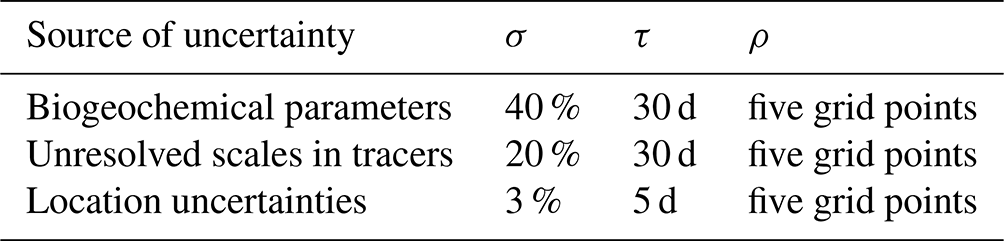
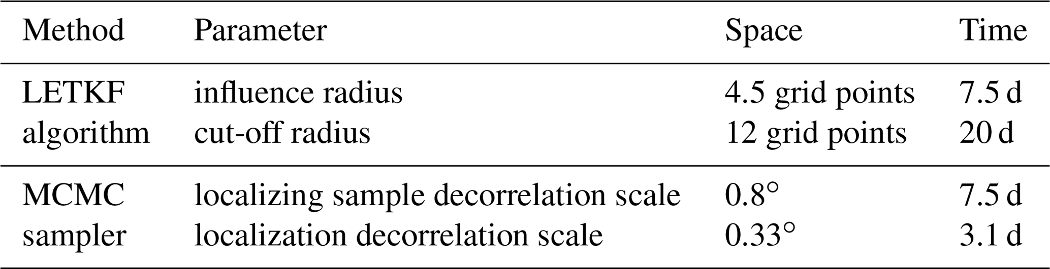
These uncertainties are all simulated using two-dimensional maps of autoregressive processes (drawn independently for each uncertainty and each parameter), whose characteristics are given in Table 1 (consistently with what was done in the papers cited above). Of course, we do not expect that they encompass all possible sources of uncertainty in the model. In the paper, this assumption about uncertainties will be used as an attempt to make the stochastic simulator consistent with the available observations. However, the validity of the assumption cannot be checked for non-observed variables, as for instance the ecosystem indicators, as further explained in the discussion of the results in Sect. 5.3.

Table 1 Characteristics of the maps of autoregressive processes used to simulate each type of uncertainty: standard deviation (σ), correlation timescale (τ), and correlation length scale (ρ). The horizontal correlation is obtained by applying a smoothing operator.

2.3 Ensemble experiment

An ensemble experiment has been performed to sample the probability distribution described by the stochastic NEMO–PISCES simulator. The sample size has been set to 40 ensemble members, which amounts to performing 40 model simulations from the same initial condition and with independent random processes in the stochastic parameterization.

The ensemble simulation has been performed for the whole year 2019 and the model results have been stored every day (at least for our region of interest) for both the physical and biogeochemical components.

3 Inverse problem

Using the statistics of the prior ensemble described in the previous section, the target is now to produce an ensemble analysis and forecast of the evolution of the ecosystem. This is formulated as an inverse problem, in which the probability distribution described by the prior ensemble is conditioned on observations. The purpose of this section is to describe the problem that is going to be solved in the paper: (i) the subregion and variables of interest (in Sect. 3.1), (ii) the Bayesian formulation of the problem (in Sect. 3.2), (iii) the observations (in Sect. 3.3), and (iv) the characteristics of the prior ensemble in the region of interest with a comparison to observations (in Sect. 3.4).

3.1 Region and variables of interest

In this study, the focus will primarily be on the analysis and forecast of the surface chlorophyll concentration, which is the observed quantity (see below). Second, we will examine how this result translates to other depth levels and to non-observed quantities, like zooplankton and particulate organic matter. Third, attempts will be made to see if more advanced diagnostics or indicators about the evolution of the ecosystem can be directly obtained as a solution of the 4D inverse problem: (i) the timing of the bloom for phytoplankton and zooplankton (phenology), (ii) the part of the primary production that is converted into secondary production (vertically integrated trophic efficiency), and (iii) the part of the resulting organic material that is trapped in the ocean (downward flux of particulate organic matter at 100 m depth).

To illustrate the approach, the inverse problem will be limited to (i) a small subregion in the North Atlantic, between 31 and 21^∘ W in longitude and between 44 and 50.5^∘ N in latitude; (ii) a 3-month time period between 15 March and 15 June 2019, including the spring bloom; (iii) a depth range between the ocean surface and 220 m depth; and (iv) a small subset of the PISCES state variables, together with a few diagnostic quantities (e.g. the vertically integrated trophic efficiency and the downward flux of particulate organic carbon, regarded as two ecological indicators of interest; see Sect. 5.3) that are introduced in the augmented state vector. As compared to classic sequential data assimilation (like the ensemble Kalman filter), the difference here is that the whole 3-month time sequence is packed together in the 4D estimation vector. This makes the problem bigger but also allows us to concentrate on a small subregion and a few selected variables. In terms of size, this amounts to 40×40 grid points in the horizontal, 32 depth levels, and 93 time steps (days), for typically six three-dimensional variables and two two-dimensional variables, so that the total size of the estimation vector x is $n=\mathrm{40}\times \mathrm{40}\times \mathrm{93}\times (\mathrm{6}\times \mathrm{32}+\mathrm{2})=\mathrm{28}\mathrm{867}\mathrm{200}$. This size is kept small enough to make the 4D inverse problem easily tractable at reasonable numerical cost.

3.2 Formulation of the problem

The 4D inverse problem is formulated using the standard Bayesian approach. First, we assume that we have a prior probability distribution p^b(x) for the estimation vector x (with dimension n as defined above). In our case, this prior distribution is defined by the stochastic NEMO–PISCES simulator described in Sect. 2. Second, we assume that we have a vector of observations y^o, which is related to the true value x^t of the estimation vector by ${\mathit{y}}^{\mathrm{o}}=\mathcal{H}\left({\mathit{x}}^t\right)+{\mathit{ϵ}}^{\mathrm{o}}$, where ℋ is the observation operator and ϵ^o is the observation error. The observation error is specified by the conditional probability distribution p[y^o|ℋ(x)], which describes the probability of an observation for a given value of x. From these two inputs, we can obtain the posterior probability distribution p^a(x) for the estimation vector (i.e. conditioned on observations) using the Bayes theorem:

$$\begin{array}{}\text{(1)}& p^{\mathrm{a}}\left(\mathit{x}\right)=p\left[\mathit{x}|{\mathit{y}}^{\mathrm{o}}\right]\propto p^{\mathrm{b}}\left(\mathit{x}\right)p\left[{\mathit{y}}^{\mathrm{o}}\left|\mathcal{H}\right(\mathit{x})\right].\end{array}$$

Our purpose throughout this paper is to solve the 4D inverse problem by producing a sample of this posterior distribution.

For further reference in the paper, it is useful to take the logarithm of this equation and define the cost function J(x):

$$\begin{array}{}\text{(2)}& J\left(\mathit{x}\right)=J^{\mathrm{b}}\left(\mathit{x}\right)+J^{\mathrm{o}}\left(\mathit{x}\right),\end{array}$$

where $J^{\mathrm{b}}\left(\mathit{x}\right)=-\log p^{\mathrm{b}}\left(\mathit{x}\right)$ is the background cost function; $J^{\mathrm{o}}\left(\mathit{x}\right)=-\log p\left[{\mathit{y}}^{\mathrm{o}}\right|\mathcal{H}\left(\mathit{x}\right)]$ is the observation cost function; and $J\left(\mathit{x}\right)=-\log p^{\mathrm{a}}\left(\mathit{x}\right)+K$, where K is a non-important constant. Ratios in probability densities translate into differences in cost functions. The larger the cost function J(x), the smaller the posterior probability.

The main difficulty with solving this problem comes from the large dimension of the estimation vector x (n=28 867 200) and the small dimension of the prior ensemble (m=40), so that specific methods with dedicated approximations are needed (see Sect. 4). This will not go without a partial reformulation of the inverse problem. First, the undersampling of the prior distribution will always require solutions to avoid the spurious effect of non-significant long-range correlations, either by solving the problem locally (domain localization) or by adjusting the prior correlation structure (covariance localization). Second, assumptions will also be needed on the shape of the probability distributions. For instance, if we can assume that both p^b(x) and p[y^o|ℋ(x)] are Gaussian and that ℋ is linear, then both J^b and J^o are quadratic, so that J is also quadratic, and a linear observational update algorithm can be used to obtain a sample of p^a(x) from a sample of p^b(x). Two options that can potentially be activated in operational systems are considered here: one using a linear algorithm (ETKF), in which all distributions are assumed to be Gaussian, and one using a nonlinear iterative algorithm (MCMC sampler), in which only p^b(x) need be assumed Gaussian (to generate appropriate random perturbations efficiently) but not p[y^o|ℋ(x)] and p^a(x). Both will require applying a transformation operator (anamorphosis) to the original variables (which are not Gaussian).

3.3 Observations

The observations y^o, which are used as conditions in the inverse problem (1), are surface chlorophyll concentrations derived from ocean colour satellites, as provided in the CMEMS catalogue (Globcolour L3 product). They are available as daily images at a $\mathrm{1}/\mathrm{24}{}^{\circ }$  resolution, as illustrated in Fig. 1 between 22 and 27 May 2019 for our region of interest. We see that the coverage is very partial in space and time as a result of the presence of clouds masking the ocean surface.

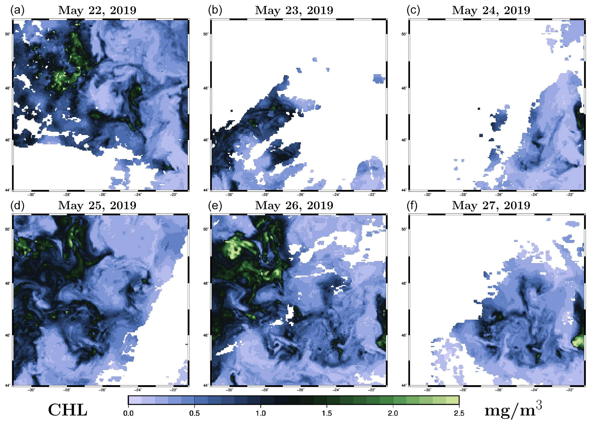
Figure 1 Observation of surface chlorophyll concentration (in mg m⁻³, L3 ocean colour product) between 22 and 27 May 2009. The x axis and y axis represent longitude and latitude, respectively.

Since chlorophyll concentration is one of the PISCES variables included in the estimation vector x, the observation operator ℋ is just a linear interpolation from the model grid to the location of observations. For the observation error probability distribution p[y^o|ℋ(x)], we assume lognormal marginal distributions, with a standard deviation equal to 30 % of the true value of the concentration, and we neglect observation error correlations. To make the assumption of zero observation error correlation more reasonable, we applied a data thinning to the original data, by subsampling the data by a factor 3 in each direction. With this reduction, the total size of the observation vector y^o over the 3 months of the experiment is p=182 837. However, when used for verification purpose, we always keep the full resolution of the observations, and the total size of the observation vector is then $p^{\prime }=\mathrm{1}\mathrm{643}\mathrm{150}$.

If the inverse method requires a Gaussian observation error probability distribution, then an approximation is required as explained in Sect. 4 and in the appendices.

3.4 Prior ensemble in the region of interest

The prior distribution p^b(x) in the inverse problem (1) is described by a sample provided by the ensemble simulation presented in Sect. 2. Figure 2 illustrates the distribution obtained for the chlorophyll surface concentration in our region of interest for 26 May 2019. The figure displays three members of the ensemble (panels a–c) and three quantiles (20 %, 50 % and 80 %) of the marginal ensemble distributions (panels d–f). For a 40-member ensemble, this means for instance that, at a given location, there are 8 members below the 20 % quantile, 8 members above the 80 % quantile, and 24 members in between.

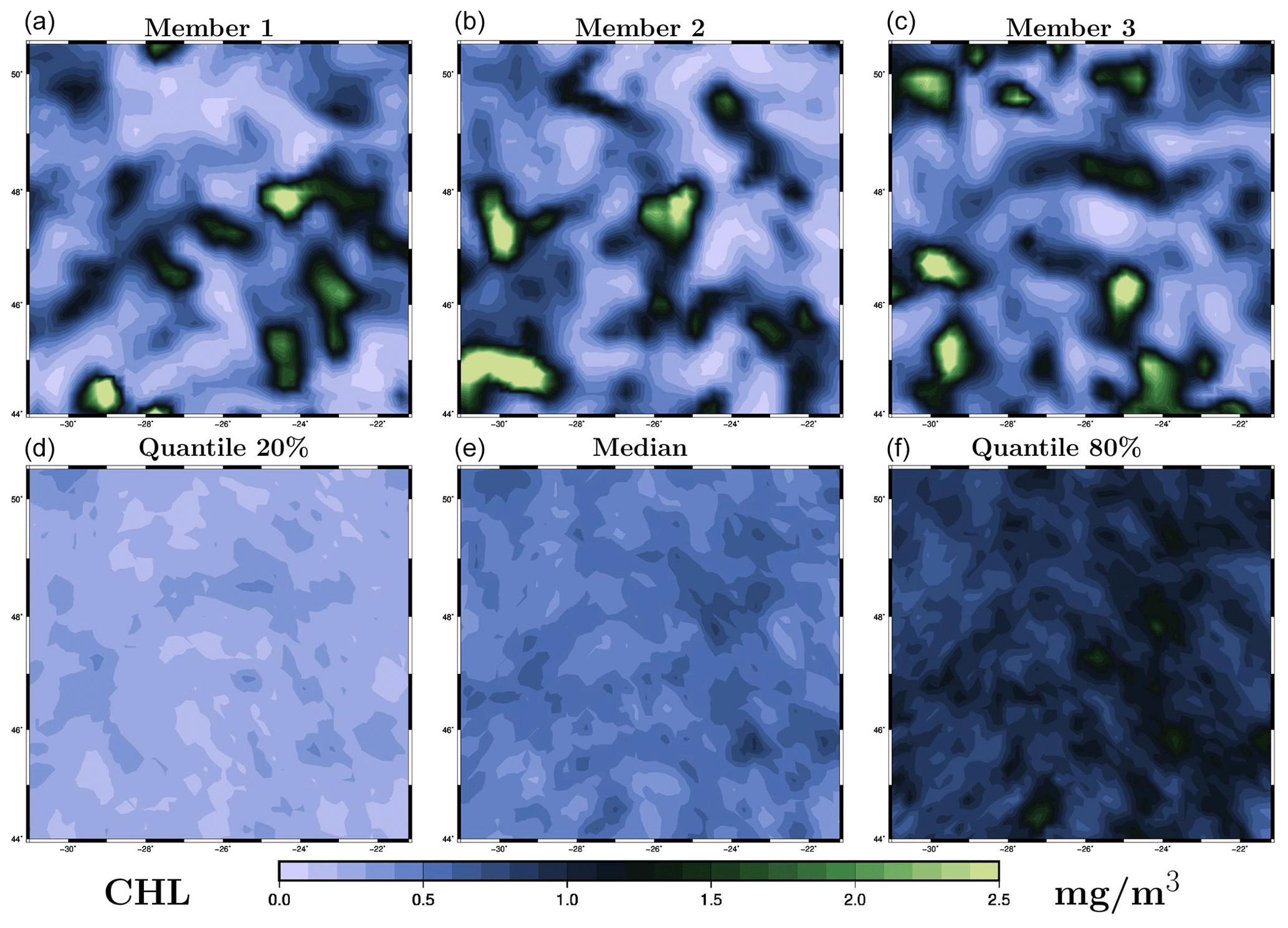
Figure 2 Prior ensemble for surface chlorophyll concentration (in mg m⁻³) on 26 May 2009. The figure displays three members of the ensemble (a, b, c) and three quantiles (20 %, 50 % and 80 %) of the marginal ensemble distributions (d, e, f). The x axis and y axis represent longitude and latitude, respectively.

From this figure, we can see that the spread of the prior ensemble, which results from the uncertainties embedded in the NEMO–PISCES simulator, is very substantial as compared to the median value (50 % quantile). Ensemble members also display a variety of patterns, which are triggered by the space and time decorrelation of the stochastic perturbations. If we compare this to the observations obtained for 26 May in Fig. 1 (panel e), we can see that the ensemble members have a comparable order of magnitude, and a large part of the observations fall in the range defined by the 20 % and 80 % quantiles.

Actually, to be consistent with the observations, the ensemble simulation should behave in such a way that 50 % of the observations are above the median, 60 % between the 20 % and 80 % quantiles, etc. More generally, an ensemble of size m defines m+1 intervals in which an observation can fall, and there should be an equal probability for the observation to fall in each of these intervals. This is the basis of the rank histogram approach to test the consistency of an ensemble simulation with observations. The histogram of all ranks of observations in the corresponding intervals defined by the ensemble should be flat (equal probability for an observation to fall in any of the intervals). More precisely, in the presence of observation errors, the ensemble members must be randomly perturbed with a noise sampled from the observation error probability distribution before computing the ranks.

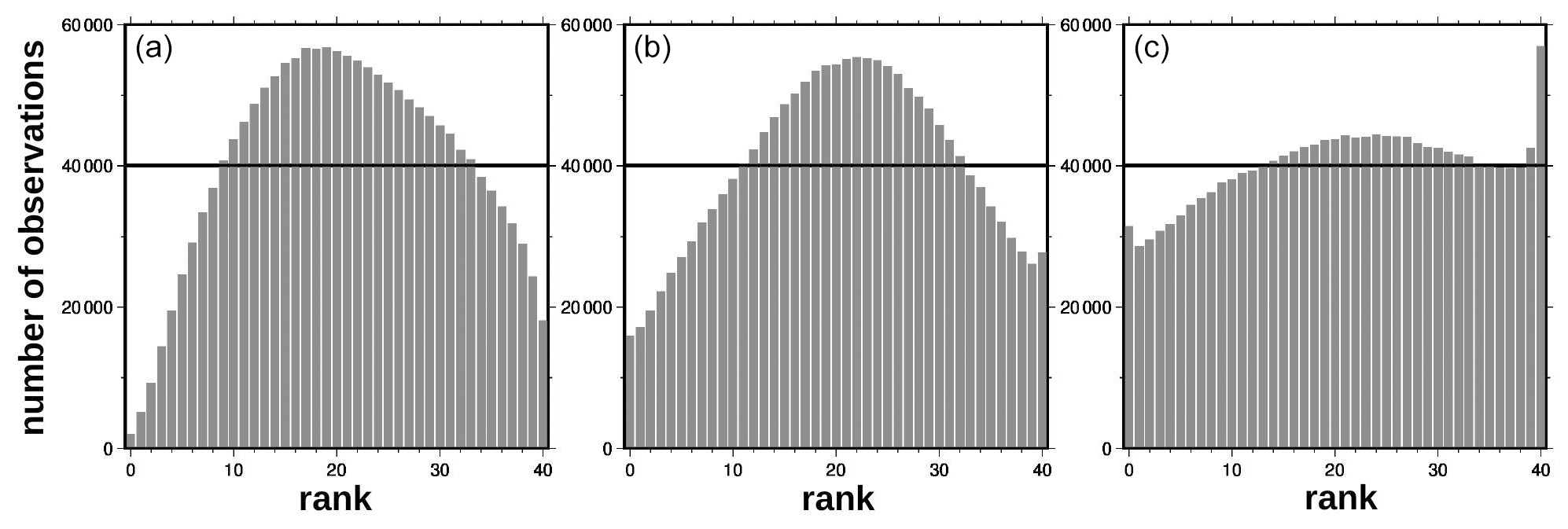
Figure 3 Rank histograms corresponding to the prior ensemble (a) and to the posterior ensemble as obtained with the LETKF algorithm (b) and the MCMC sampler (c). For the posterior ensembles, the histograms aggregate ranks from two simulations: one conditioned on observations from the odd days only, which is validated using observations from the even days, and another one conditioned on observations from the even days only, which is validated using observations from the odd days.

Figure 3a shows the rank histogram obtained for the prior ensemble using all observations in our region of interest during the 3-month time period (i.e. with $p^{\prime }=\mathrm{1}\mathrm{643}\mathrm{150}$ observations). We can see that this histogram is not flat: the ensemble simulation is overdispersive here. Uncertainties in the model have been overestimated: there are too many observations close to the median of the ensemble and not enough in the external intervals defined by the ensemble. It would certainly be better if the rank histogram could have been perfectly flat, but an underdispersive ensemble would have been much worse. Underestimating prior uncertainties would indeed mean that the dynamical ensemble simulation has not explored regions of the state space corresponding to the observed values, and the solution of the inverse problem would imply positioning the posterior probability distribution in these regions where the prior probability is zero and where we have no dynamical information about the behaviour of the system. Such an extrapolation might be possible for the observed variable but would be very hazardous for non-observed quantities.

It must be noted that, in the prior simulation described in Sect. 2, there are other regions and/or seasons where the ensemble is still very underdispersive and/or biased, with most observations falling outside of the range of possibilities explored by the model. In the Atlantic, this occurs for instance in most of the subtropical gyre and on the southern edge of the Gulf Stream extension. In such a situation, the methods used in this paper would not be effective, and it is first necessary to improve the description of uncertainties in the prior model simulation.

4 Inverse methods

To solve the inverse problem described in the previous section, we show that several methods can be used in a versatile way. In the present demonstration, two methods will be applied: (i) the first one is the analysis step of the ensemble transform Kalman filter (ETKF) proposed in Bishop et al. (2001), with domain localization (e.g. Janjic et al., 2011); (ii) the second one is the implicitly localized MCMC sampler proposed in Brankart (2019). The two methods provide a solution to the same problem and produce an updated ensemble, which is meant to be a sample of the posterior probability distribution (conditioned on the observations). But they use different algorithmic choices and different types of approximation, which are described in the rest of this section. Note that other updating methods could have been considered, such as EnKF, 3D-Var, etc. In Sect. 4.1, we describe the general algorithms that are used to perform the observational update (a Kalman filter and an MCMC sampler) and the level of generality that they achieve. In Sect. 4.2 and 4.3, we highlight what the two schemes imply in terms of localization scheme and anamorphosis transformation, respectively.

4.1 Observational update algorithm

In Kalman filters (like the ETKF), the mean and covariance of the updated ensemble are computed from the mean and covariance of the prior ensemble using linear algebra formulas involving the observation vector, the observation operator and the observation error covariance matrix. This relies on the assumption that both prior and posterior distributions, as well as observation errors, are Gaussian and that the observation operator is linear. If put in square-root form (as the ETKF), the scheme directly uses and provides the square root of the covariance matrix (possibly with a low rank), which is equivalent to using and providing an ensemble description of the covariance matrix. Our specific implementation of this algorithm is inherited from the SEEK filter (Pham et al., 1998), which is another square-root filter, with an analysis step that can easily be made equivalent to that of the ETKF (especially once it has been adapted to allow for domain localization, as in Brankart et al., 2003; Testut et al., 2003).

By contrast, MCMC samplers are iterative methods, which converge towards a sample of the posterior probability distribution. Our particular implementation is a variant of the Metropolis–Hastings algorithm (see, e.g., Robert and Casella, 2004), which is designed in such a way that the stochastic process, which generates the next element of the Markov chain, is in equilibrium with the probability distribution that must be sampled. This is obtained by an iteration in two steps: (i) one step to draw a random perturbation from a proposal probability distribution and (ii) one step to accept or reject this new draw according to the variation in the cost function. In this respect, our variant (Brankart, 2019) is somehow specific in the sense that (i) the proposal distribution is based on the prior ensemble (with covariance localization; see below) and (ii) only the observation component of the cost function is needed to evaluate the acceptance criterion. Because of this, the method still requires that the prior probability distribution be Gaussian, but no assumption is made here on the shape of the posterior probability distribution or on the observation constraint, which can be nonlocal, nonlinear, and even non-differentiable.

4.2 Localization

In ensemble Kalman filters, localization is used to alleviate the effect of a small ensemble size as compared to the number of degrees of freedom in the system. In terms of covariance, the main negative effect of an insufficient sample size is that low correlations are typically overestimated (for instance, zero correlations are approximated by non-zero correlation), which can produce a substantial spurious effect on the results. Localization can be obtained with two different approaches: (i) domain localization (e.g. Janjic et al., 2011), in which the solution at a given location is computed using observations only within a specified neighbourhood (with a decrease in the observation influence with the distance to avoid discontinuities), and (ii) covariance localization (e.g. Houtekamer and Mitchell, 1998), in which the ensemble covariance is transformed by a Schur product with a local-support correlation matrix (thus zeroing the long-range correlations). In both cases, it is assumed that the ensemble size is sufficient to describe the covariance structure when considered locally.

In square-root Kalman filters (like the ETKF and SEEK filters), covariance localization is difficult to apply because the ensemble covariance is never explicitly computed, only the square root is available. A solution has nevertheless been proposed by Bishop et al. (2017) in the framework of the ETKF, which consists in transforming each column of the covariance square root by a Schur product with each column of a square root of the localizing correlation matrix. The resulting matrix can be shown to be a square root of the localized covariance matrix, which is what is needed by the square-root algorithm. However, with this approach, the number of columns of the square-root covariance, and thus the cost of the resulting algorithm, is considerably increased (multiplied by the number of columns in the square root of the localizing correlation matrix). This is why, in the application below, we still use the more simple domain localization for the ETKF algorithm (as in the MOI operational system).

In the MCMC sampler, covariance localization can be introduced using a very similar approach as in the ETKF. If we assume that we can easily sample a zero-mean Gaussian distribution with the localizing correlation structure, then we can define the sampling of the proposal distribution using the Schur product of one member of the prior ensemble (anomaly with respect to the mean) with one member of this localizing sample. This provides the time–space pattern of the perturbation, which is then multiplied by a Gaussian random factor (with a standard deviation equal to 1). From the same property used by Bishop et al. (2017) for the ETKF, the perturbation will have the same covariance as the prior ensemble, with covariance localization. However, in this different context, the large increase in the number of directions of perturbation associated with localization becomes a benefit, since we want the perturbations to explore the estimation space as much as possible to fit the observations and produce the posterior sample. Moreover, if the localizing correlation can itself be expressed as the Schur power of a specified correlation matrix, it is again possible to produce a very large sample (up to 10⁸−10¹²) with the localizing correlation from a small sample (typically 10²) with the specified correlation, just by computing the Schur product of a random combination of elements from the small sample (see Brankart, 2019, for more details). With the localization method, the sampling of the proposal distribution in many dimensions is thus reduced to the computation of a multiple Schur product with randomly selected members from a small sample, at a cost that is linear in the size of the system. This is important because this cost is usually quadratic and thus often a limiting factor to the application of MCMC samplers in large-dimension problems.

4.3 Anamorphosis

Anamorphosis (𝒜) is a nonlinear transformation that is applied to a model variable x to transform its marginal probability distribution into a Gaussian distribution (with zero mean and unit variance). It is useful because many data assimilation methods (like the two methods presented here) make the assumption of a Gaussian prior distribution. In this paper, we use the simple anamorphosis algorithm described in Brankart et al. (2012), which consists in remapping the quantiles of the marginal distribution of x on the quantiles of the target Gaussian distribution, using a piecewise linear transformation (interpolating between the quantiles). The transformed variable $x^{\prime }=\mathcal{A}\left(x\right)$ is then approximately Gaussian.

However, as explained above, Kalman filters also require that the observation operator is linear and that the observation error is Gaussian. In this case, a similar transformation must also be applied to observations to keep the observation operator linear in the transformed variables. This can be done using the algorithm described in the appendices. This algorithm provides the right expected value and error variance for the transformed observation, but the detailed shape of the observation error probability distribution is lost by the transformation, since the observation error on this transformed observation must be Gaussian. It is indeed impossible to find a transformation that ensures Gaussianity of both the prior and observational uncertainties, while keeping the observation operator linear.

By contrast, in the MCMC sampler, it is not required that the observation operator is linear, so that the observations do not need to be transformed. The original observation operator ℋ needs only to be complemented by an inverse anamorphosis transformation 𝒜⁻¹, to come back from the transformed vector x^′ to the original vector x: ℋ(x) is just replaced by $\mathcal{H}\left[{\mathcal{A}}^{-\mathrm{1}}\right({\mathit{x}}^{\prime }\left)\right]$. This makes the use of anamorphosis much easier since only the estimation variables need to be transformed and not the observations. The observation constraint can be applied using the native observations, with the native observation operator and the native observation error probability distribution.

5 Results

In this section, we describe the solution obtained for the inverse problem formulated in Sect. 3 using the methods presented in Sect. 4. The focus will be on evaluating the reliability and accuracy of the ensemble analysis and forecast using dedicated probabilistic scores. The section is first devoted to the results obtained for the observed variable (the surface chlorophyll concentration), in terms of analysis (Sect. 5.1) and forecast (Sect. 5.2), and then extended to discuss the results obtained for non-observed variables and ecosystem indicators (Sect. 5.3).

5.1 Analysis for observed variables

To illustrate first the idea of a single ensemble analysis extending over a long time period (3 months), Fig. 4 shows time series of the surface chlorophyll concentration at the centre of the region of interest (47.25^∘ N, 26^∘ W), as obtained with the two methods: the LETKF (localized ETKF) algorithm (panel a) and the MCMC sampler (panel b). The black curves represent 40 members of the prior ensemble (as produced by the NEMO–PISCES simulator) and the blue curves represent 40 members of the posterior ensemble (conditioned on all observations available in the period). We can see that the prior uncertainty in these time series is considerably reduced by the observations. For instance, at this location, the timing of the spring bloom was left very uncertain by the NEMO–PISCES simulation, probably because it is very dependent to the uncertain parameters that have been perturbed. But, even if partial and imperfectly accurate, the observations contain a lot of information about this, so that the variety of possibilities left in the posterior ensemble is much smaller (with both methods). In this respect, it must already be noted that the solution at a given time is influenced by both past and future observations. This is an important advantage over sequential ensemble filters, in which only past observations can influence the solution obtained at a given time.

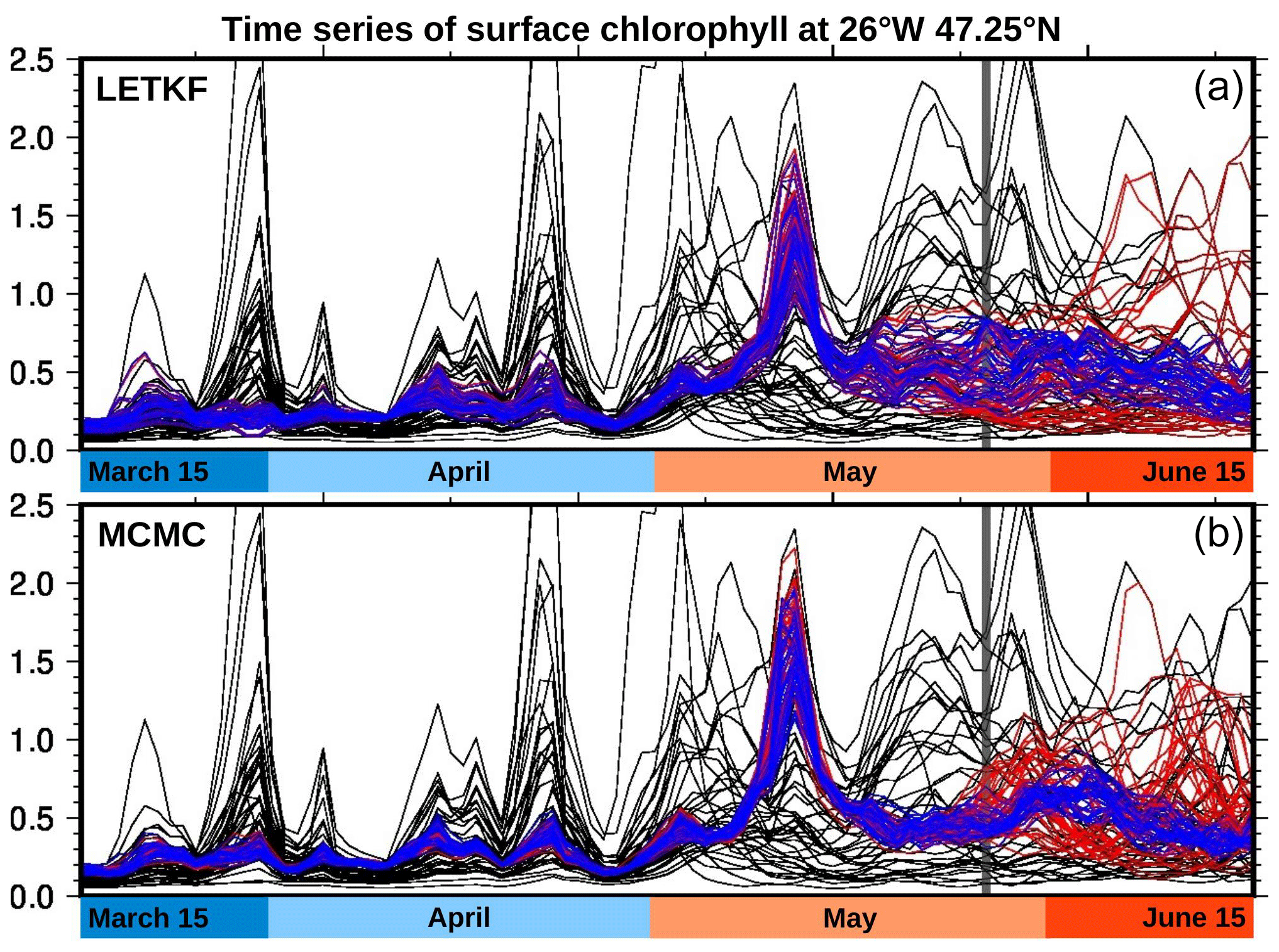
Figure 4 Ensemble surface chlorophyll time series at 47.25^∘ N, 26^∘ W. The black curves represent 40 members of the prior ensemble (as produced by the NEMO–PISCES simulator), the blue curves represent 40 members of the ensemble analysis (using observations for the entire period), and the red curves represent 40 members of the ensemble forecast (using only observations until 25 May). The forecast thus starts on 25 May (vertical grey line). These results are shown for the LETKF algorithm (a) and the MCMC sampler (b).

Second, to illustrate the resulting maps of surface chlorophyll concentration, we choose to focus on 26 May 2019, when there is a good coverage of observations (see Fig. 1), with which the results can be compared. For this date, Fig. 5 (LETKF algorithm) and Fig. 6 (MCMC sampler) display three members of the posterior ensemble (panels a–c) and three quantiles (20 %, 50 % and 80 %) of the posterior marginal ensemble distributions (panels d–f). This gives an idea of individual possibilities and of the spread of the ensemble and can be directly compared to the same information provided for the prior ensemble in Fig. 2. Again, we can see that, with both methods, the spread of the ensemble is considerably reduced by the observation constraint, with all posterior members getting closer to the observed situation. Even if there are differences between methods (see discussion below), most observed structures are present in the two ensemble analyses. In both cases, however, there remains a variety of possibilities in terms of location and amplitude of the structures, as a result of the substantial uncertainty in the observations (a 30 % observation error standard deviation). At first glance, despite the use of completely different algorithms (LETKF and MCMC sampler), the two ensemble analyses are generally reasonable and quite similar. They can thus be discussed together in more detail.

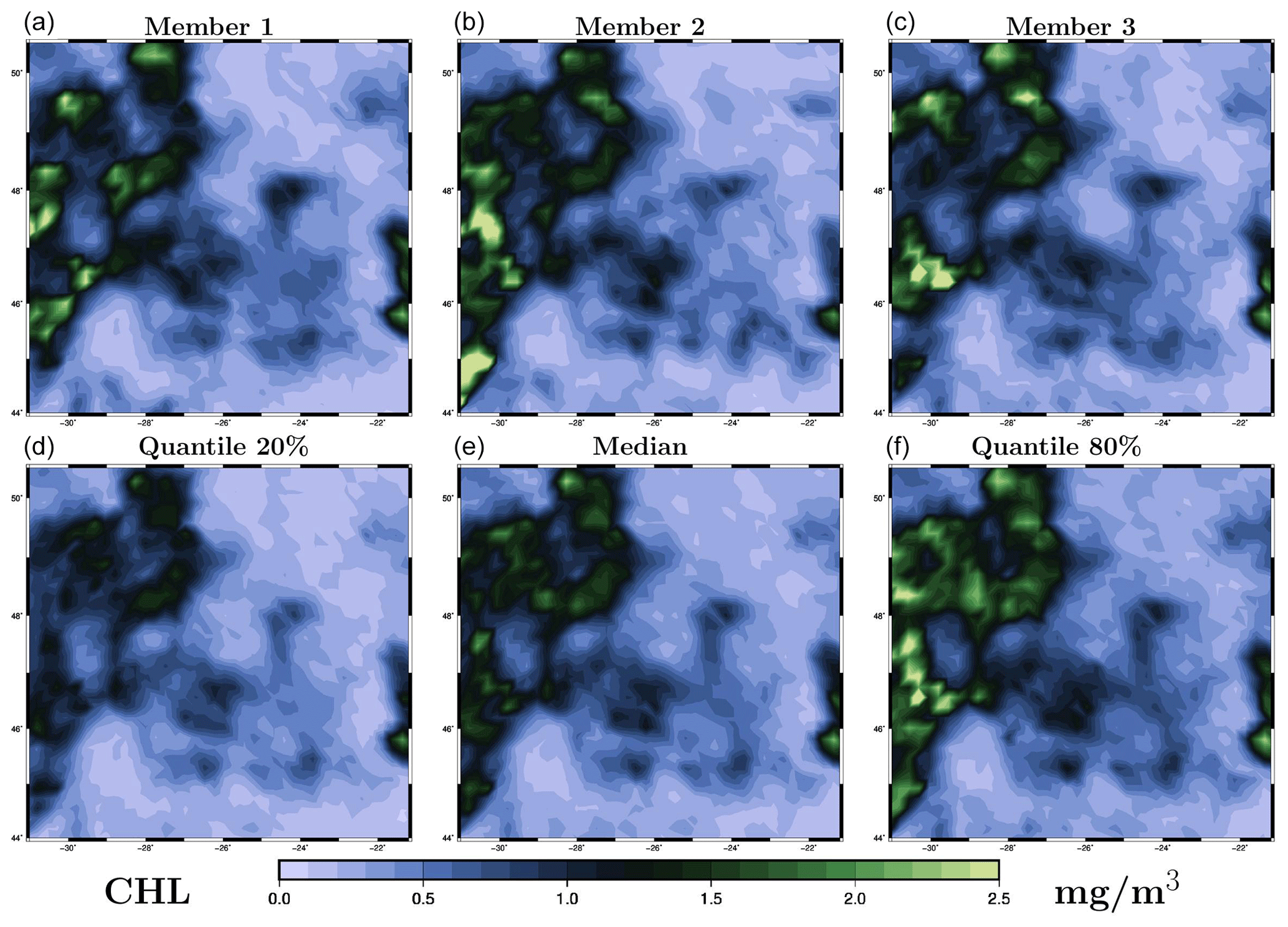
Figure 5 Ensemble analysis obtained with the LETKF algorithm for surface chlorophyll concentration (in mg m⁻³) on 26 May 2009. The figure displays three members of the ensemble (a–c) and three quantiles (20 %, 50 % and 80 %) of the marginal ensemble distributions (d–f). The x axis and y axis represent longitude and latitude, respectively.

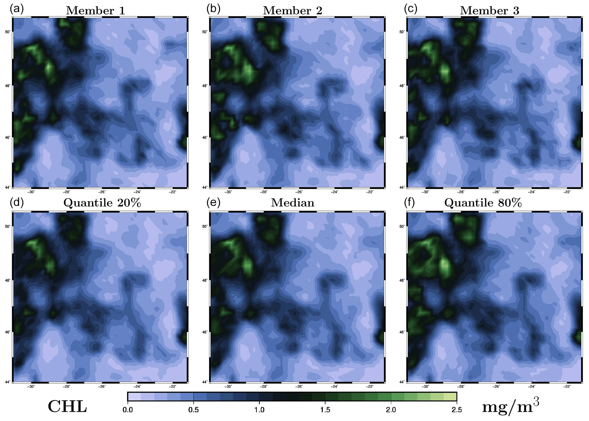
Figure 6 Ensemble analysis obtained with the MCMC sampler for surface chlorophyll concentration (in mg m⁻³) on 26 May 2009. The figure displays three members of the ensemble (a–c) and three quantiles (20 %, 50 % and 80 %) of the marginal ensemble distributions (d–f). The x axis and y axis represent longitude and latitude, respectively.

5.1.1 Space and time localization

Regarding the formulation of the inverse problem, the main difference between the two solutions is the localization scheme, which also contains the only free parameters of the inverse algorithm (i.e. not included in the definition of the problem in Sect. 3). The localization parameters used in our experiments are given in Table 2. In both cases, we have to specify a length scale and a timescale, but there is no direct correspondence between the parameters used in the two algorithms because their behaviour is not the same. In principle, they must be set so that the effect of remote observations vanishes when the ensemble correlation becomes non-significant, but this always requires some additional tuning.

Table 2 Localization parameters used in the LETKF algorithm and in the MCMC sampler. In the LETKF algorithm, the localizing function is set to be isotropic (with a Gaussian-like shape) in the metrics defined by the grid of the model. In the MCMC sampler, the localizing correlation is set to be isotropic on the sphere (degrees are along great circles); the localizing sample is generated using a Gaussian spectrum in the basis of the spherical harmonics (in the horizontal) and a Gaussian spectrum in the basis of the harmonic functions (in time), so that the sample correlation structure is also Gaussian and the localizing correlation structure as well. There is no localization along the vertical coordinate.

Not enough localization means that remote observations keep too much influence: the fit to local observation is lost, the ensemble spread is too small, and the solution thus becomes unreliable. Too much localization means that relevant remote observations are missed, the ensemble spread is too large, and the solution becomes inaccurate. In our experiments, localization has been tuned heuristically to obtain a good compromise on the scores presented below: a sufficient ensemble spread to keep the solution reliable (rank histogram) and a good fit to independent observations (probabilistic score) in the analysis and in the forecast. Regarding the local structure of the solution, we can see, by comparing Figs. 5 and 6, that covariance localization tends to be more respectful of the local correlation structure of the prior ensemble (by construction), while domain localization can trigger small scales that are not present in the prior ensemble. There are situations in which this can make a big difference, but this may not be so important in the present application.

5.1.2 Reliability

The most important property of the analysis results is the reliability of the ensemble, i.e. the consistency with independent verification data. This can be evaluated using rank histograms as explained in Sect. 3.4 for the prior ensemble. To keep independent surface chlorophyll observations, we performed two additional analysis experiments: one using observations from the odd days only, which we can validate using observations from the even days, and another one using observations from the even days only, which we can validate using observations from the odd days. By aggregating the ranks of the verification data from these two experiments, we can obtain a rank histogram based on all available observations, as was done for the prior ensemble.

Figure 3 displays the rank histogram obtained for the ensemble analysis performed with the LETKF algorithm (panel b) and with the MCMC sampler (panel c). In both cases, the resulting ensemble is not underdispersive, except for a very small excess of observations above the maximum of the ensemble in the case of the MCMC sampler. Underestimating the posterior uncertainty is never a good idea, and this can be directly avoided here by tuning the localization parameters until the posterior ensemble spread is sufficient (which is always possible, as long as the prior ensemble is itself reliable). Regarding this particular diagnostic, the localization of the LETKF could have been tuned towards less localization to decrease the spread of the posterior ensemble and make the overall rank histogram flatter. However, it must be kept in mind that this diagnostic aggregates a variety of different situations in space and time and that other diagnostics also matter (e.g. the reliability of the forecast; see below).

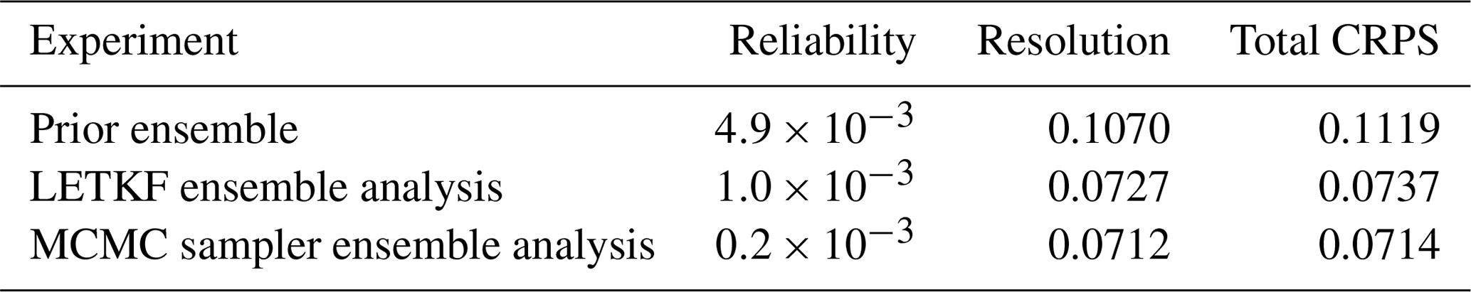
Table 3 Global CRPS (in mg m⁻³), using all available surface chlorophyll observations over the full time period of the experiments. The scores of the analyses aggregate the scores from two simulations: one using observations from the odd days only, which is validated using observations from the even days, and another one using observations from the even days only, which is validated using observations from the odd days.

5.1.3 Probabilistic scores

To further compare the ensemble analysis with verification data, we must not only check the consistency between the results and the data but also quantify the amount of information that the analysis provides about the data. This is done here using the continuous ranked probability score (CRPS), which is defined from the misfit between the marginal cumulative distribution function (cdf) of the ensemble (regarded as a stepwise function increasing by $\mathrm{1}/m$ at the value of each ensemble member) and the cdf associated with the corresponding observation (regarded as a Heaviside function, increasing by 1 at the value of the observation). The CRPS can be decomposed as the sum of a reliability component (characterizing the consistency between the ensemble and the observations) and a resolution component (characterizing the amount of information provided by the ensemble). Roughly speaking, if the misfit is due to observations falling systematically outside of the range of the ensemble, it will contribute to the reliability component of the score. Conversely, if the misfit is due to the spread of the ensemble, it will contribute to the resolution component of the score. In the case of Gaussian variables, the gain of information brought by the observations (i.e. the resolution component of the score) is often characterized by variance ratios, which could have been computed here for the transformed variables (by anamorphosis). But we have preferred providing an assessment of the original concentration variable using the CRPS.

Table 3 provides the value of the score obtained for the prior ensemble and for the analysis obtained by each of the two methods. Again, in the case of the analyses, the score is an aggregate computed from two different experiments, so that only independent observations are used to evaluate the scores. From the table, we see that the total score and the resolution component of the score are very similar with the two methods. Moreover, it must be noted that the contributions to this score are quite heterogeneous in space and time, with none of the methods systematically outperforming the other in terms of CRPS misfit.

In terms of reliability, the score obtained with the MCMC sampler ($\mathrm{0.2}\times {\mathrm{10}}^{-\mathrm{3}}$ mg m⁻³) is here better than that obtained with the LETKF algorithm ($\mathrm{1.0}\times {\mathrm{10}}^{-\mathrm{3}}$ mg m⁻³), but the two results can be regarded as sufficiently good, as a direct result of the tuning of the localization parameters. In this respect, it must also be noted that more accurate observations would make a more stringent test of reliability. With large observation uncertainties, the necessary conditions of reliability tested with these scores are more easily achieved.

5.1.4 Numerical cost

Table 4 provides the numerical cost of the two analysis experiments (with the LETKF and the MCMC sampler). A comparison of the computational complexity of the two algorithms as a function of the size of the problem is presented in Brankart (2019). It is here just briefly particularized to our application. From this table, we can see that, as applied in this study, the MCMC sampler is about 6.5 times more expensive than the LETKF algorithm. But this directly depends on choices that have been done in terms of parameterization and implementation.

Table 4 Dimension of the problem and cost of the analysis experiments. The time to read input data and write output data is not included in the clock time.

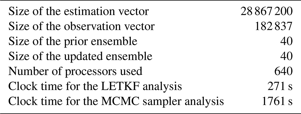
In both algorithms, the computational complexity is linear in the size of the estimation vector (n) and in the size of the observation vector (p), so that this has no influence on their relative cost. In the LETKF, the cost is quadratic in the size of the updated ensemble, which must be the same as the size of the prior ensemble (m). Moreover, the cost is also proportional to the volume of the space–time domains used by the localization algorithm (defined by the cut-off length scale and timescale in Table 2). For given influence scales, this domain is difficult to reduce without risking space–time discontinuities in the resulting fields. In the MCMC sampler, the cost is linear in the size of the updated ensemble (m^′), which can be different from the size of the prior ensemble (m). This is an advantage because it is possible to compute only a few members at a much smaller cost (for example eight members at a cost 5 times smaller) and then compute more and more members as deemed useful for a given application (for example 200 members at a cost 5 times larger). But the cost is also proportional to the number of iterations N needed to reach the solution. This makes the cost of the MCMC sampler much less predictable than the cost of the LETKF algorithm because this depends on the number of degrees of freedom that must be controlled and the level of accuracy required. In the experiments performed for this paper, N is set to 30 000 to be sure that the convergence has been reached. But experiments done with N=10 000 iterations do not show a very substantial difference in the scores and in the results; the distance to the observations is only slightly larger. And the cost is reduced to a third of what is given in Table 4).

In terms of implementation, it must also be noted that the MCMC sampler is much easier to code and parallelize that the LETKF algorithm. Providing that the ensemble equivalent to the observations is provided as an input, each processor can deal separately with a block of the state vector and a block of the observation vector, with almost no communication between them, except the summation of the distributed components of the cost function (and a few other scalar quantities like the random coefficient to the global perturbation). This is possible in this algorithm because the inverse problem is solved globally and because covariance localization is obtained implicitly through global Schur products, computed separately in estimation space (to iterate the solution, with random perturbations) and in observation space (to compute the corresponding perturbations and evaluate the cost function).

5.2 Statistical forecast

If we now reduce the observation vector to include only observations before a given time t₀, the result of the inverse problem can be interpreted as an ensemble analysis before t₀ and an ensemble forecast after t₀. This forecast is a time extrapolation based on the statistics of the prior ensemble, with space and time localization. In our case, it is a nonlinear statistical forecast, since it is based on the linear space–time correlation structure for nonlinearly transformed variables (by anamorphosis). Figure 4 (red curves) shows the result obtained with the LETKF algorithm (panel a) and the MCMC sampler (panel b), when the last date of observation is 25 May 2019 (as represented by the vertical grey line in the figure). In both cases, the spread of the posterior ensemble increases during the forecast, and starts increasing before t₀ when the lack of future observations begins. At t₀ indeed, only half of the observations used in the analysis are available (as would also be the case for the ensemble analysis in a sequential Kalman filter).

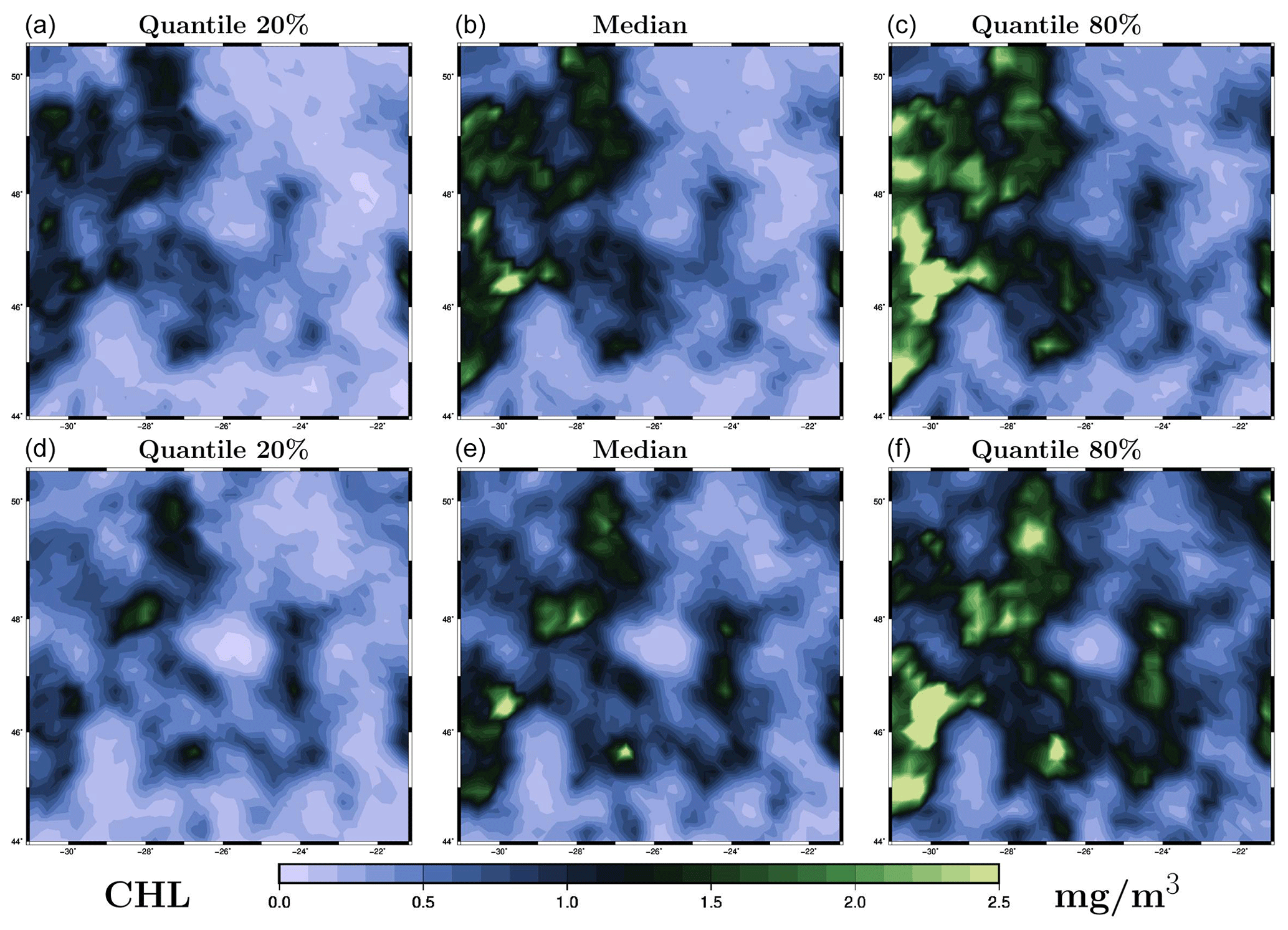
Figure 7 Ensemble forecast obtained with the LETKF algorithm for surface chlorophyll concentration (in mg m⁻³) on 26 May 2009. The figure displays three quantiles (20 %, 50 % and 80 %) of the marginal ensemble distributions, as obtained for the 1 d forecast (a–c) and the 4 d forecast (d–f). The x axis and y axis represent longitude and latitude, respectively.

Regarding the future (t>t₀), we see that extrapolation in time is much more sensitive to the particulars of the localization method. In the LETKF algorithm (with domain localization), the problem is solved locally and separately for each time (and each horizontal location), and the influence of the past observations (before t₀) decreases with time as a result of the time decorrelation present in the prior ensemble and the superimposed localizing influence functions (as parameterized by the influence radii). This influence is then cut off when the local domain does not include t₀ anymore (in our case, at t₀+20 d, when the posterior members become exactly equal to the prior members). In the MCMC sampler (with covariance localization), the problem is solved globally for the whole time period and the influence of past observations (before t₀) decreases with time as a result of the time decorrelation present in an augmented version of the prior ensemble, whose covariance is localized by a Schur product with a localizing correlation function. This influence thus vanishes with time, but there is no cut-off time here, since there is no boundary to the domain of influence. These differences explain why the forecast can behave somewhat differently in the solution produced by the two methods.

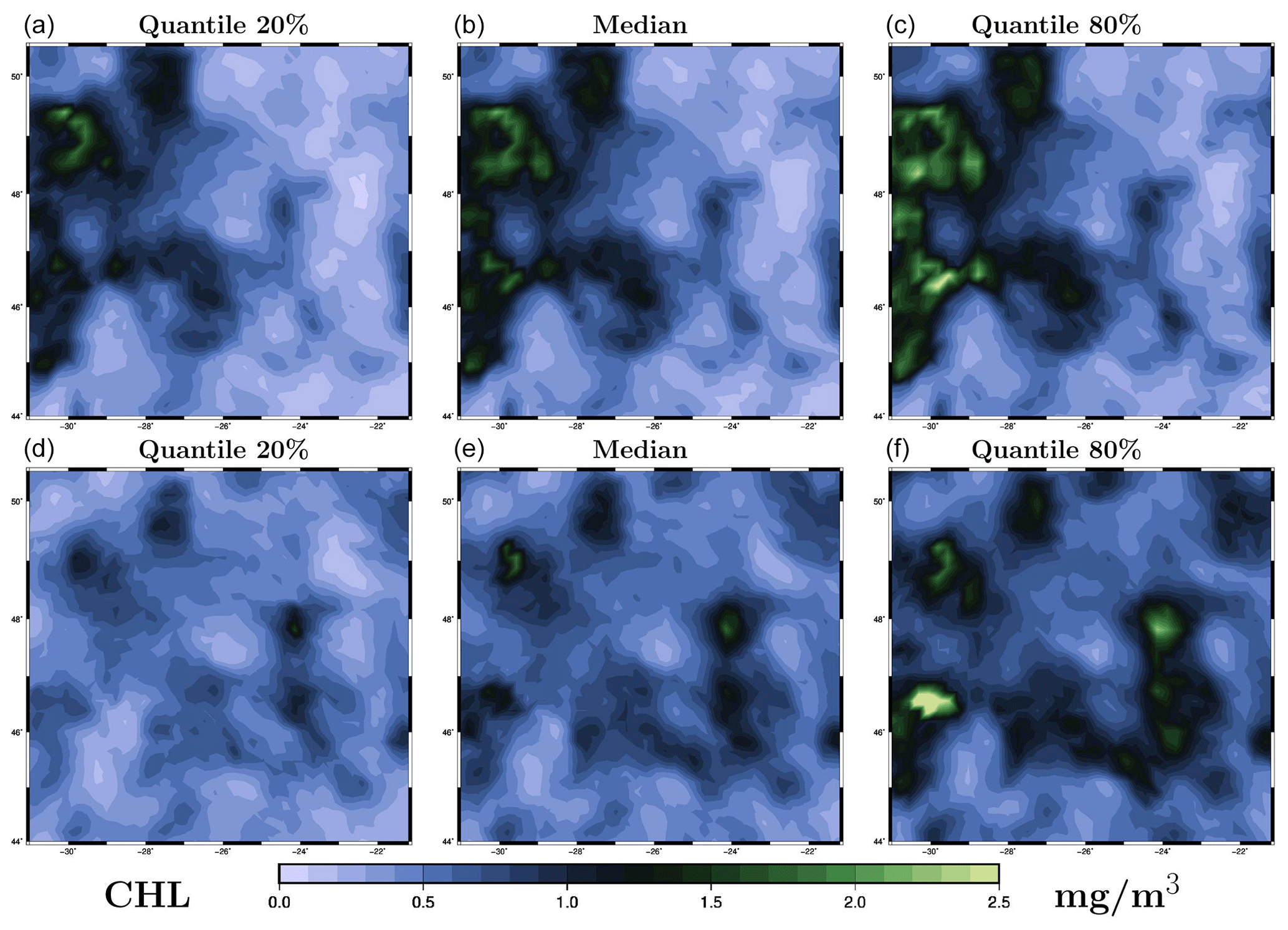
Figure 8 Ensemble forecast obtained with the MCMC sampler for surface chlorophyll concentration (in mg m⁻³) on 26 May 2009. The figure displays three quantiles (20 %, 50 % and 80 %) of the marginal ensemble distributions, as obtained for the 1 d forecast (a–c) and the 4 d forecast (d–f). The x axis and y axis represent longitude and latitude, respectively.

5.2.1 Forecast accuracy

To further evaluate the forecast, we consider two ensemble forecasts obtained for the same date (26 May 2019), but with a different time lag with respect to the last observation. The first one is a 1 d forecast, with the last observation on 25 May 2019 (Fig. 1d), and the second one is a 4 d forecast, with the last observation on 22 May 2019 (Fig. 1a). The date of the forecast (26 May) is chosen so that the results can be directly compared to the observations in Fig. 1 (panel e), to the prior ensemble in Fig. 2, and to the ensemble analyses in Fig. 5 (LETKF algorithm) and in Fig. 6 (MCMC sampler). The ensemble forecast is described by three quantiles (20 %, 50 % and 80 %) of the marginal distributions, as shown in Fig. 7 (for the LETKF algorithm) and in Fig. 8 (for the MCMC sampler). The two figures include the 1 d forecast (panels a–c) and the 4 d forecast (panels d–f).

In these figures, we can see that the accuracy of the forecast deteriorates with time, and the spread of the ensemble increases accordingly. After 1 d, the ensemble forecast is still very similar to the ensemble analysis and the observations (not used anymore in the inversion problem). Only a few structures are missing from the median, and the ensemble spread is not that much larger (see the scores below for a more precise quantification). After 4 d, the situation becomes more fuzzy. The forecast still contains valuable information, and we can still recognize the main patterns of the observed surface chlorophyll concentration, but most local structures are missed or not correctly positioned. The posterior uncertainty described by the ensemble spread is also substantially larger but still much smaller than the prior uncertainty. These general features of the 1 and 4 d ensemble forecasts are shared by the two methods, but there are also differences in their behaviour. On the one hand, the LETKF algorithm tends to keep more small-scale structures and extreme chlorophyll concentrations (both low and high values), which are inherently more uncertain and require a larger spread. On the other hand, the MCMC sampler tends to produce a smoother solution (consistently with the prior ensemble) with less extreme values, which leads to sometimes missing the possibility of small-scale structures in the forecast. This different behaviour of the two methods can be attributed to the difference in the space–time localization algorithm.

About the respective accuracy of the 1 and 4 d forecasts, it is important to remark that the conclusions drawn above are not general. They depend on the correlation structure of the prior ensemble, which may be very heterogeneous in space and time, and on the availability of observations. For instance, in our case study, if we look at the observation coverage in Fig. 1, we see that we have one good observation coverage 1 d before 26 May and another one 4 d before 26 May, which is why we decided to illustrate the results with a 1 and a 4 d forecast. In this example, the 2 d forecast or the 3 d forecast would have been no better than the 4 d forecast since there are only very few observations available on 23 and 24 May. The capacity to make a forecast is obviously dependent on the availability of observations. In addition, it must be noted that our case study is not strictly speaking a forecast, since we used a prior ensemble simulation in which the atmospheric forcing is based on a reanalysis. For our experiment to be a real forecast, the prior simulation should have used an atmospheric forecast rather than a reanalysis. This would not be a difficulty in an operational context, and it is not likely to make a big difference in the illustration presented in this paper (at least for the short-term forecast).

5.2.2 Probabilistic scores

Table 5 provides a more quantitative assessment of the forecast, with the probabilistic scores obtained for 26 May 2019, i.e. using all surface chlorophyll observations available on that day. The scores are given for the 1 and 4 d forecasts and compared to the scores obtained for the prior ensemble and the analysis, always on the same day. In addition to the CRPS (reliability and resolution), we have also computed the RCRV score (reduced centred random variable), which is a measure of the reliability of the ensemble (and thus says nothing about the resolution) in terms of bias and spread (Candille et al., 2007; Candille et al., 2015). More precisely, the reduced variable is defined as the misfit between each piece of verification data and the corresponding ensemble mean, and then normalized by the ensemble standard deviation. If the ensemble is reliable, the expected value of this reduced variable (bias) must be 0 and its standard deviation (spread) must be 1 % or 100 %. If the bias is positive (negative), this means that the ensemble is systematically too small (too large) as compared to the verification data. If the spread of the reduced variable is too large, above 100 % (below 100 %), this means that the spread of the ensemble is too small (too large) to be consistent with the verification data. As for the CRPS, if the verification data are observations, the ensemble must be perturbed by the observation error before computing the score.

Table 5 CRPS (in mg m⁻³) and RCRV score (in %) for 26 May 2019. Since this is an odd day in the time sequence, the scores of the analyses come from the experiment using observations from the even days only, so that the observations used for validation are independent.

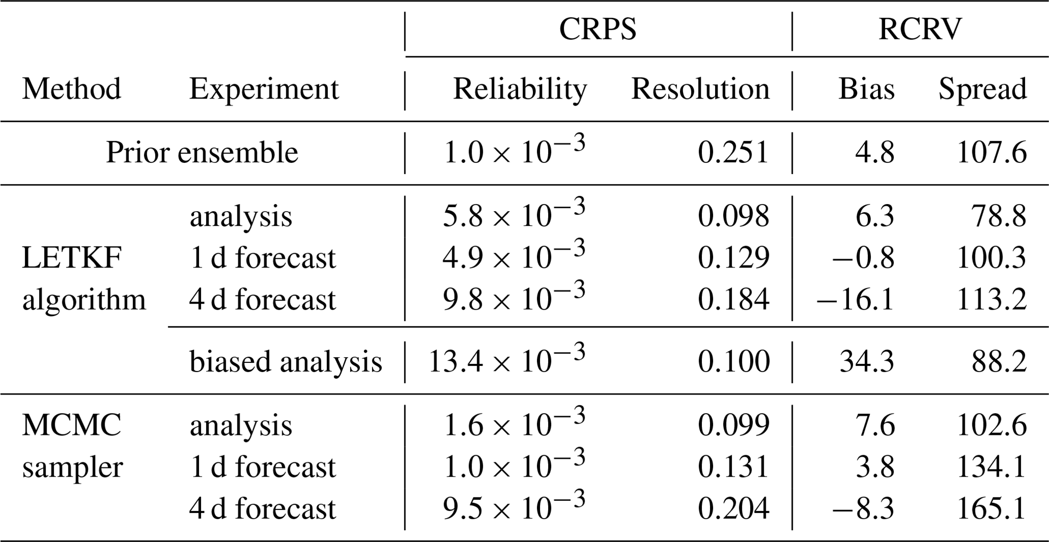
The figures of the scores provided in Table 5 show first that the prior ensemble and the analyses (LETKF and MCMC) are quite reliable for that date, with biases well below 10 % of the ensemble spread and a quite accurate ensemble spread, as confirmed by the low value of the CRPS reliability component. The largest misfit to reliability is in the LETKF analysis, which is somewhat overdispersive. Regarding the forecast, the 1 d forecast is still as reliable as the analysis, except for the MCMC 1 d forecast, which is somewhat underdispersive (134 % RCRV spread). In terms of resolution, with a score of about 0.13 mg m⁻³, the 1 d forecast is not very far from the analysis (about 0.1 mg m⁻³) and still much better than the prior ensemble (about 0.25 mg m⁻³). By contrast, in the 4 d forecast, both reliability and resolution degrade substantially. The bias grows to about −16 % (for the LETKF algorithm) and −8 % (for the MCMC sampler), and the MCMC ensemble forecast becomes even more underdispersive (165 % RCRV spread). This is confirmed by their larger CRPS reliability score, which is similar but presumably for different reasons (one because of the larger bias and the other because of the underdispersion of the ensemble). As already observed in Figs. 7 and 8, the forecast also contains much less information than the analysis, with a CRPS resolution growing to about 0.18 mg m⁻³ for the LETKF algorithm and 0.20 mg m⁻³ for the MCMC sampler but still substantially better than the prior ensemble (about 0.25 mg m⁻³).

In order to illustrate the importance of correctly applying the observation constraint when observation errors are non-Gaussian, we have added one line of scores in Table 5 for the LETKF algorithm (named “biased analysis”). In this biased analysis, the algorithm is exactly the same except that the anamorphosis transformation of the observations is performed using the simplified algorithm in Annex A1, rather than the more general algorithm in Annex A2, which is much needed in our application. With the simplified algorithm, there is indeed a strong bias on the ensemble analysis (about one-third of the ensemble spread), in which the chlorophyll concentration is systematically too small as compared to the observations. The CRPS reliability score is also substantially increased, but the nature of the problem is less apparent with this score. In our problem, this spurious effect is large because the observation errors are large, but it is important to remain cautious when a Gaussian approximation of non-Gaussian observation errors is needed, as in Kalman filters (with or without anamorphosis). There is no such difficulty with the MCMC sampler, in which the observation constraint can be applied using the native observation error probability distribution. This special attention to observation errors was only needed on the LETKF side to make the level of reliability of the two solutions coincide.

5.3 Ecosystem indicators

Up to now, the ensemble analysis and forecast have been diagnosed in terms of the observed variable only. In the following, we move to the diagnostic of non-observed quantities, starting with variables that can be expected to be well controlled by the observations towards ecosystem indicators that are more likely to depend on uncontrolled processes: (i) the phenology of the bloom, (ii) the vertically integrated trophic efficiency, and (iii) the downward flux of particulate organic matter at 100 m depth.

5.3.1 Phenology

As a simple characterization of the phenology of the spring bloom (at a given location in 3D), we use the first date at which the chlorophyll concentration reaches half of its maximum value (at that particular location) over the whole time period. This definition has the advantage of being as closely related to the observations as possible and of not being too sensitive to small uncertainties in the value of the concentrations. Unlike the maximum, it is indeed likely to occur at a time of strong time derivative of the concentration. Figure 9 shows the resulting description of phenology for the surface chlorophyll concentration, as obtained for the prior ensemble (panels a–c), the LETKF analysis (panels d–f), and the MCMC sampler analysis (panels g–i). The figure displays quantiles of each of these ensembles (from left to right: 20 %, 50 % and 80 %). It is important to emphasize here that phenology has been computed first for each ensemble member, and then the quantiles have been derived from the phenology ensemble, not the other way around. The result is a probability distribution for phenology, which we describe by a few quantiles. In the figure, we can see that the prior uncertainty in phenology is quite large and that this uncertainty is strongly reduced by the observation constraint, in a way that is very similar in the two methods.

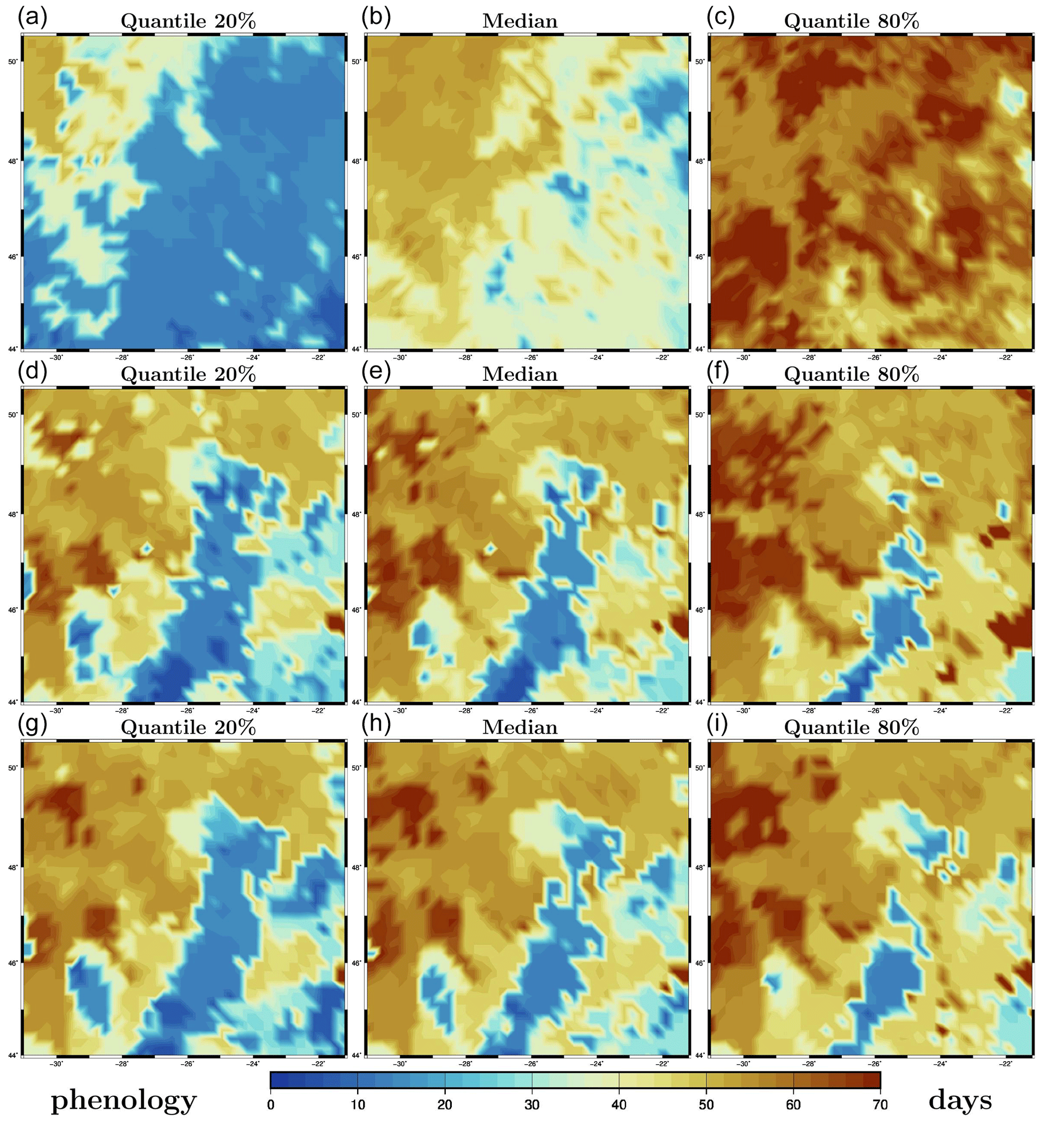
Figure 9 Quantiles of phenology (in days). Prior ensemble (a–c), LETKF analysis (d–f), and MCMC sampler analysis (g–i). The x axis and y axis represent longitude and latitude, respectively.

Furthermore, from the ensemble experiments, it is possible to explore if the phenology of chlorophyll is linked to the phenology of zooplankton (using the same definition as above). Figure 10 shows a scatter plot of these two dates at the same location already used for Fig. 4 (47.25^∘ N, 26^∘ W surface value, at the centre of the region). The figure compares the result obtained with the LETKF algorithm (panel a) and the MCMC sampler (panel b). The figure displays members of the prior ensemble (black dots) and of the ensemble analysis (blue dots). The small black dots in panel b represent members of an augmented version of the prior ensemble (200 members), with covariance localization. It is obtained with the MCMC sampler, used exactly as for the analysis (at a much lower cost) but without the observation constraint. It is more representative of the prior ensemble that is actually used by the MCMC sampler, since it includes localization.

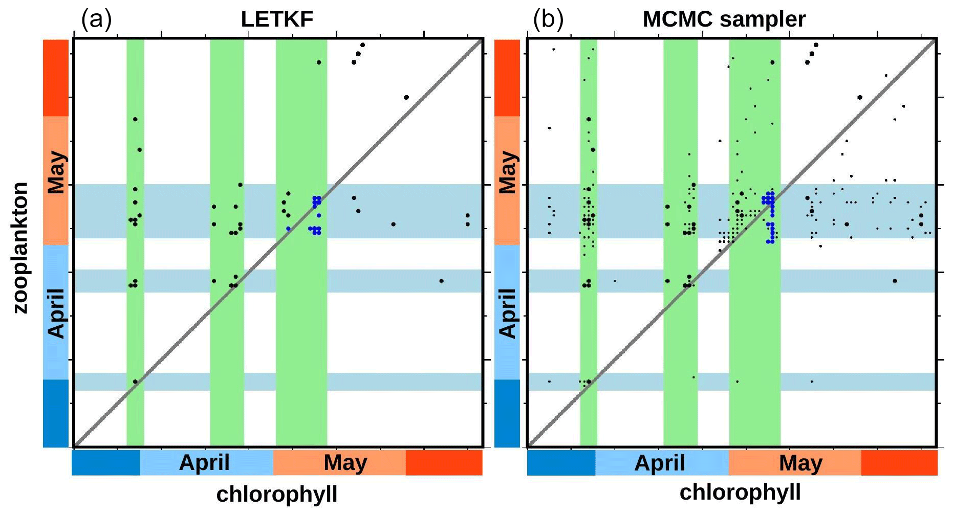
Figure 10 Scatter plot of phenology (in days) for chlorophyll (x axis) and zooplankton (y axis). At 47.25^∘ N, 26^∘ W. With the LETKF algorithm (a) and the MCMC sampler (b). Prior ensemble (black), augmented prior (small black dots), and analysis (blue).

In the figure, we can see that the prior ensemble mainly opens three possible time windows in which chlorophyll phenology can take place. They are represented in the figure by the three light green areas, which can be seen to correspond to peaks of the prior surface chlorophyll concentration in Fig. 4. These three windows can presumably be associated with favourable conditions offered by the physical forcing (in terms of light, temperature, and/or mixing) for the phytoplankton bloom to occur. The specific phenology in each member then depends on how the biogeochemical model behaves, as a function of the stochastic perturbation applied to each of them. From these three modes of the prior distribution, the observation constraint makes the ensemble analysis select just the third one, in which the posterior probability is concentrated (with both methods). Correspondingly, the phenology of zooplankton displays the same three windows in the prior ensemble (in light blue in Fig. 10), with a small general shift forward in time. But the posterior uncertainty is here larger: ±5 d for zooplankton rather than ±1 d for chlorophyll (at this location).

About the posterior uncertainty in the phenology of zooplankton, it must be emphasized that this largely depends on the assumptions that have been made to describe the prior uncertainties. For instance, in the prior ensemble simulation described in Sect. 2, uncertainties in the grazing of phytoplankton by zooplankton have not been taken into account. These uncertainties may have an influence on the dependence between the behaviours of phytoplankton and zooplankton and thus increase uncertainties in the phenology of zooplankton, as compared to what is shown in Fig. 10.

5.3.2 Trophic efficiency

Trophic transfer efficiency (or trophic efficiency) measures the part of energy that is transferred from one trophic level to the next and is a common indicator used to characterize food availability to high trophic level organisms of economic or ecological importance and, for instance, how this availability is affected by environmental changes (Eddy et al., 2021). Trophic efficiency is usually computed as the ratio of production at one trophic level to production at the next lower trophic level. However, since those specific diagnostics are rarely recorded explicitly, it is common to use the ratio between the biomass of upper and lower trophic levels as a proxy measure of the trophic transfer efficiency within the food web (Armengol et al., 2019; Eddy et al., 2021). Here, trophic efficiency is evaluated as the ratio between the biomasses of primary producers and consumers vertically integrated over the 0–200 m layer.

The computation of this indicator first requires vertical profiles of phytoplankton and zooplankton, and this depends on the ability of the inverse methods to extrapolate the surface information in depth. Figure 11 displays vertical profiles of chlorophyll concentration (panels a and c) and microzooplankton concentration (panels b and d), as obtained with the LETKF algorithm (panels a and b) and the MCMC sampler (panels c and d). It is shown for the same location as in Fig. 10 (47.25^∘ N, 26^∘ W, at the centre of the region) and for the median date obtained for the chlorophyll phenology (day 55, 8 May) in the ensemble analyses. By virtue of the anamorphosis transformation, all posterior ensemble members gently follow the same general vertical structure as the prior ensemble, without overshooting or obvious inconsistent behaviours. Only the spread of the ensemble is reduced, towards values that are somewhat different in the two methods. At that date and location, the chlorophyll concentration is larger with the MCMC sampler, and the microzooplankton concentration is smaller.

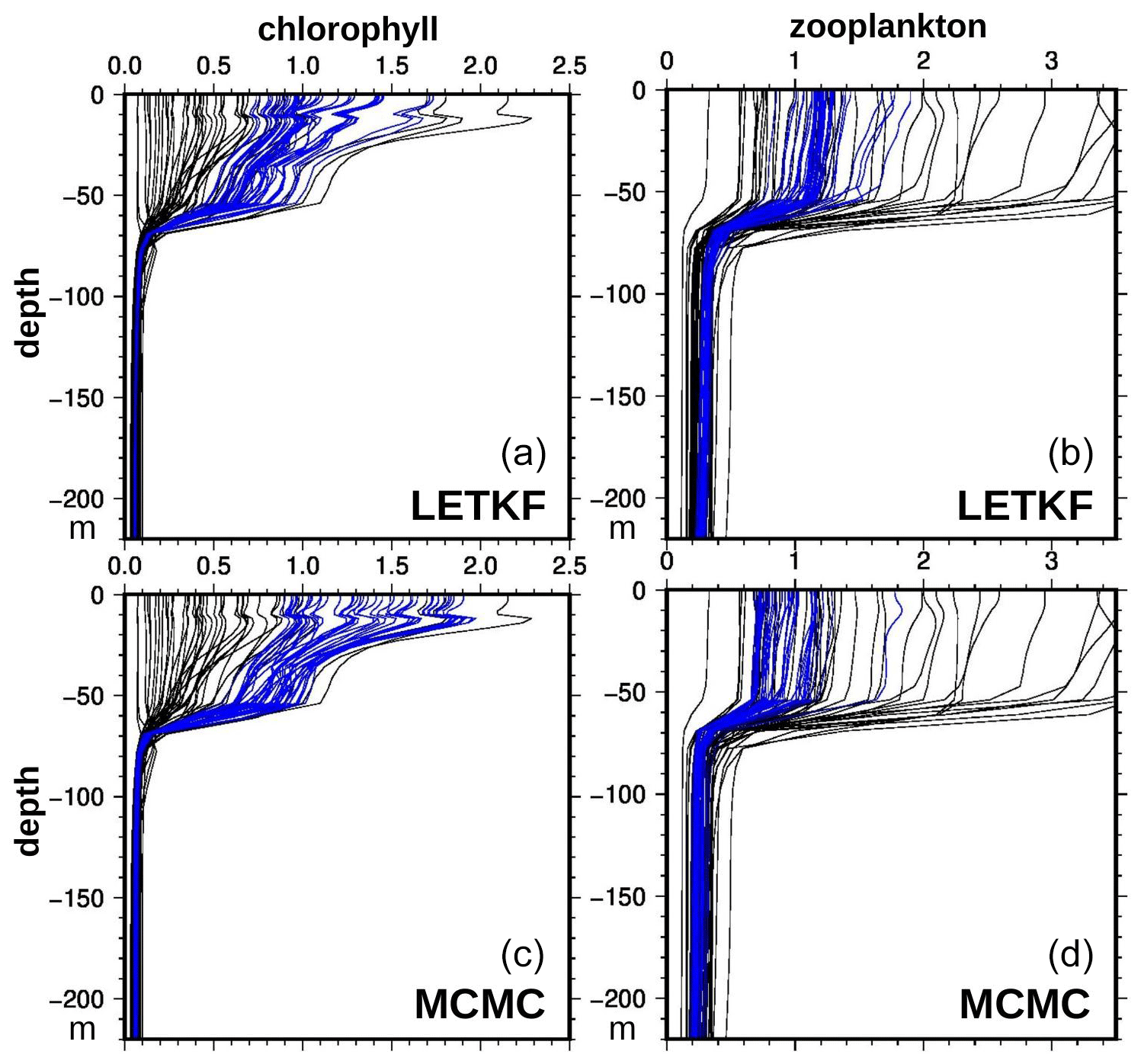
Figure 11 Vertical profile of chlorophyll (in mg m⁻³, a, c) and microzooplankton (in mmol C m⁻³, b, d). At 47.25^∘ N, 26^∘ W, 8 May 2019. With the LETKF algorithm (a, b) and the MCMC sampler (c, d). Prior ensemble (black) and analysis (blue).

More importantly, we see that, in all profiles, the depth of the active layer is about the same in all members, which means that we assumed no prior uncertainty on this. This can only mean that uncertainties are missing in the prior NEMO–PISCES simulator (presumably in the physical component), and the consequence is that our results probably underestimate uncertainties in the vertical integrals. In any case, these uncertainties could not have been controlled using ocean colour observations only and would have required involving other types of observations.

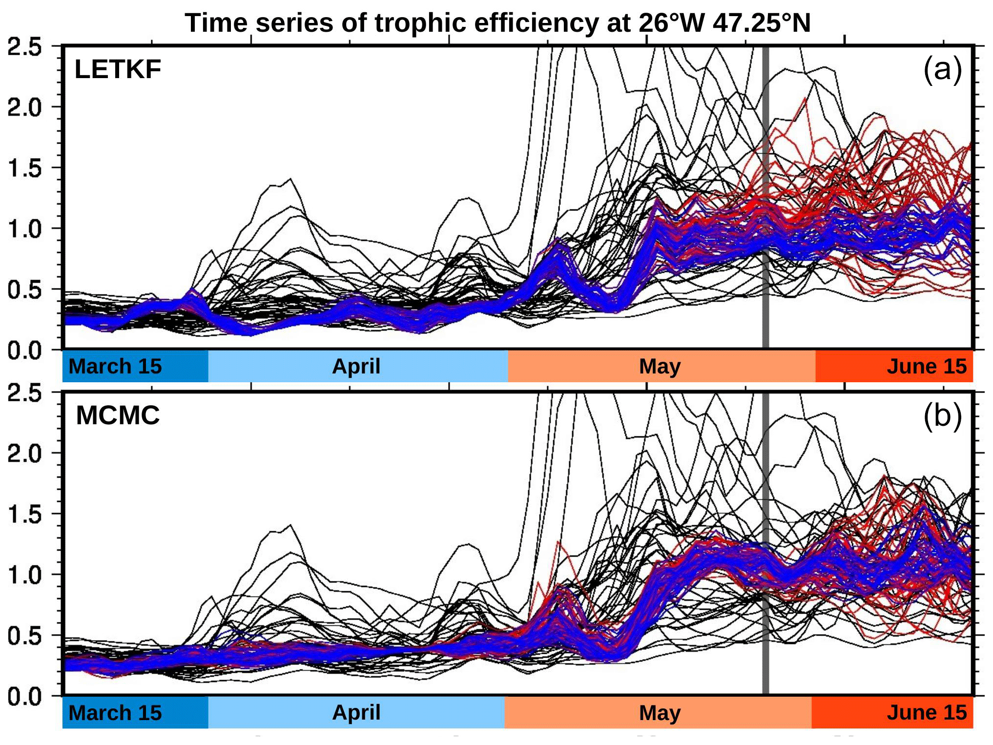
Figure 12 Time series of trophic efficiency. At 47.25^∘ N, 26^∘ W. With the LETKF algorithm (a) and the MCMC sampler (b). Prior (black), analysis (blue), and forecast (red).

With this caution in mind, Fig. 12 displays time series of the vertically integrated trophic efficiency at the same location, as obtained with the LETKF algorithm (panel a) and the MCMC sampler (panel b). The figure is organized exactly as Fig. 4, at the same location but for a different variable. From day 0 to day 60, the ratio slightly increases from 0.3 to 0.5, a range that is in line with the value given in this area by the trophic model of Negrete-García et al. (2022). After the bloom (see Fig. 4), the trophic efficiency increases towards values closer to 1 and above 1, which is indicative of a transition from a bottom–up to a top–down control of the phytoplanktonic population. In the prior ensemble, we can still distinguish the three possible windows for the occurrence of the bloom, while it is reduced to 1 in the posterior ensemble (with a smaller spread), consistently with the posterior phenology estimates. However, the quantitative accuracy and reliability of the trophic efficiency estimates entirely depend on the reliability of the prior ensemble and in particular on the reliability of the correlation between the trophic efficiency and the observed variable (see discussion at the end of Sect. 5.3.3).

5.3.3 Downward flux of particulate organic matter

The downward flux of particulate organic matter (POM) relates to the biological gravitational pump, i.e. the sinking of organic matter under direct action of gravity. It is one constituent of the biological carbon pump, which includes the ensemble of processes that transfer carbon from the surface ocean (where it is balanced with atmospheric CO2 concentration through air–sea exchanges) and deeper oceanic layers where carbon is regarded as “stored” on larger timescales (Claustre et al., 2021). There are many ongoing discussions on how to optimally infer biological carbon pump indicators from model simulations, sustained by the obvious importance of such indicators in the frame of global change (e.g. Galí et al., 2022). In our case, we stick to the simple definition of multiplying the concentrations of two classes of organic matter at the 100 m horizon (below the active layer; see Fig. 11) with their specific sinking velocities and summing up both contributions. To understand the results below, it is important to note that (i) the model simply considers fixed sinking rates (parameters) for each class of POM and (ii) those parameters are not part of the uncertainty considered to build the prior ensemble. The spread of this indicator in the prior ensemble therefore remains intimately related to that of phytoplankton production.

Figure 13 displays a scatter plot of this indicator (y axis) vs. surface chlorophyll concentration (x axis) for 26 May 2019, at the same location as before (47.25^∘ N, 26^∘ W, at the centre of the region), as obtained with the LETKF algorithm (panel a) and the MCMC sampler (panel b). The figure displays members of the prior ensemble (black dots), of the ensemble analysis (blue dots), and of the 4 d ensemble forecast (red dots). With both methods, the spread of the analysis and forecast is strongly reduced as compared to the prior ensemble. The two methods produce a similar ensemble analysis. With the MCMC sampler, the forecast is compatible with the analysis but with a larger spread. With the LETKF algorithm, however, the 4 d forecast is incompatible with the analysis. This happens to be a location at which the 4 d LETKF forecast of chlorophyll (but not the 1 d forecast) is biased as compared to the analysis. This could already have been observed in Fig. 7, where, at the centre of the region, there is a pattern with a low value of the surface chlorophyll concentration in all quantiles, which is incompatible with both the analysis and the observations. This bias in the forecast here translates into the forecast of the indicator.

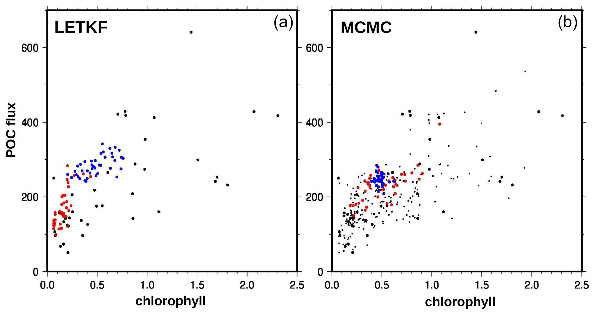
Figure 13 Scatter plot of surface chlorophyll concentration (in mg m⁻³) vs. particular organic carbon (POC) flux at 100 m depth (in mg C m⁻² d⁻¹). At 47.25^∘ N, 26^∘ W, on 26 May 2019. With the LETKF algorithm (a) and the MCMC sampler (b). Prior (black), augmented prior (small black dots), analysis (blue), and 4 d forecast (red).

The reliability of the indicator estimate depends on the reliability of the prior correlations between this indicator and the observed variable (as described by the black dots in Fig. 13). The reliability of the forecast also depends on the reliability of the time correlation (and the time localization scheme). Both depend on the modelling assumptions embedded in the NEMO–PISCES simulator. These assumptions here combine a deterministic framework (providing information about the behaviour of the system) and a stochastic parameterization (accounting for uncertainties). As in any modelling system, unreliable assumptions will produce unreliable results. For instance, in this example, we neglected uncertainties in the sinking velocities, so that the confidence in the indicator is certainly overestimated. It is even possible that no valuable information about this indicator can be obtained from surface chlorophyll only, in view of the current modelling knowledge and missing uncertainties. But the same difficulty can be expected for any complex system, in which uncertainties are often ignored or not modelled adequately, which can lead to artificially low uncertainty estimates in certain indicators.

6 Conclusions

In this paper, a simplified approach has been introduced to perform a 4D ensemble analysis describing the evolution of the ocean ecosystem. In our example, it is based on prior ensemble statistics from a stochastic NEMO–PISCES simulator and ocean colour observations. The observations are used as constraints to condition the 4D prior probability distribution. The results show that it is possible to produce an ensemble solution that is continuous in time, consistent with the observations, and with a reliable description of the posterior uncertainty (at least for the observed variable). Furthermore, attempts have been made to extrapolate the results into the future from past observations. The resulting 4D ensemble statistical forecast is shown to be most often reliable (at least for the observed variable) and to contain valuable information about the evolution of the ecosystem for a few days after the last observation. However, as a result of the short decorrelation timescale in the prior ensemble, the spread of the ensemble forecast increases quickly with time.

In terms of method, the inverse problem has been solved using two very different algorithms: the analysis step of the LETKF (with domain localization) and an MCMC sampler (with covariance localization). The performance of the two algorithms are enhanced by applying a nonlinear transformation to the estimation variables (anamorphosis). These two methods being so different from each other, the most important conclusion that can be drawn is certainly that common features displayed by the two results validate each other. Differences between the results are more difficult to interpret because it is difficult to separate the effect of the method and the effect of the tuning of localization (which cannot be made equivalent in the two algorithms). On the one hand, covariance localization (with a localizing correlation function) is more flexible, and it has a better theoretical justification, so that the Bayesian inverse problem remains global, and the local correlation structure of the prior ensemble can be preserved better. On the other hand, domain localization (with a decreasing influence function) is more like an ad hoc solution with only a few parameters, and there is no global Bayesian formulation of the problem anymore, so that there is more risk of triggering non-physical small scales when the local domain are shifted from each other (to solve the global problem piece by piece). However, in our experiments, it can happen that this simple scheme, with just a weighted decrease in the influence of the past observations, can produce a more accurate ensemble forecast but also occasionally bigger biases.

The key practical advantage of the approach presented in this study, as compared to standard data assimilation, is to decouple the resolution of the inverse problem from the application of the complex numerical model (here the NEMO–PISCES stochastic simulator), which is only used as a supplier of prior input data. This has given us the possibility of focusing on a small subregion, in which the inverse problem is well-conditioned and to solve the problem globally in time for a full 3-month time period, thus avoiding the filtering approach, in which only past observations can influence the analysis at a given time. Without the need to re-initialize the model, it has also been possible to concentrate on a few variables of interest and indicators that are not model state variables. As long as the prior ensemble statistics are reliable for a subset of the model variables, an analysis and forecast can directly be obtained for these variables and associated indicators without going through the burden of estimating the full state vector. In terms of method, this simplified approach has allowed us to try using a more general iterative algorithm to solve the problem, thus avoiding the Kalman approach, in which only linear constraints are possible (linear observation operator and Gaussian observation errors). In our results, this did not bring many improvements because much care has been taken to perform the anamorphosis transformation of the non-Gaussian observation error probability distribution required by the Kalman algorithm. But this is still an approximation, which is not necessary in the MCMC sampler. Moving to a nonlinear method, solving the problem globally, also offers new perspectives in terms of constraints that can be applied to the solution, such as nonlocal and nonlinear observation operators or nonlocal and nonlinear dynamical constraints (as long as the associated cost function is not too expensive to evaluate).

The main theoretical shortcoming of this approach is that the complex dynamical model is no longer directly used to constrain the solution. However, it must be recognized that this is not always possible in practice. As long as most of the model state variables remain unobserved (and there are 23 state variables in PISCES) and often poorly correlated to the observed variables, it can be a very difficult task to initialize properly a dynamical model forecast (or to adjust an even larger number of model parameters), especially if the model is very sensitive to small inconsistencies in the initial state. Ad hoc adjustments and simplifications are then usually needed to avoid model failure or unrealistic results. In other words, in the case of non-observability and non-controllability of the dynamical system, the problem can become ill-conditioned, and it can be worthwhile starting from a simplified approach in which these problems do not occur.

Regarding the operational applications, this approach offers the possibility of being more flexible and less dependent on the behaviour of the global data assimilation system. It can quickly focus on a specific region of interest and produce targeted products to meet dedicated users' requirements, at a small additional cost. This can be done without any new technical development, using the same algorithm already in use in the dynamical data assimilation system (e.g. the LETKF algorithm), and the simplified framework can serve as a test bed for more advanced inverse methods (e.g. the MCMC sampler).

The main condition to perform such a 4D analysis and forecast of the evolution of the ecosystem is to produce a reliable prior ensemble simulation based on the complex dynamical model. This is not an easy prerequisite, which requires identifying the most important sources of uncertainty in the system and developing stochastic perturbations schemes to take them into account. Reliability must then be checked against observations, so that the inversion can concentrate on regions where uncertainties have been sufficiently understood and where reliable products can be delivered. Concerning the non-observed variables (like the ecosystem indicators), the reliability of the results entirely depends on the assumption made to produce the prior ensemble, which must be questioned and checked wherever possible. In our results about the indicators, we have mentioned that important uncertainties have been neglected, so that the posterior uncertainty on the indicators is certainly underestimated. However, the situation is similar in dynamical forecasting systems, in which the reliability of the ensemble forecast also depends on the modelling assumptions. Any progress towards a better understanding of the model uncertainties is thus directly beneficial to both types of system.

Appendix A: Anamorphosis transformation of the observations

The following algorithms have been implemented to address the problem of transforming the observations. We first consider a simplified particular case allowing a more efficient algorithm before addressing the general problem. In both cases, the objective is to produce an unbiased transformed observation, with a consistent observation error standard deviation.

A1 The observation error probability density function is symmetric and does not dependent on the true state

In this particular case, the transformation of the probability distribution for observation error is straightforward, and can be obtained using the following algorithm for each observation (assuming independent observation errors).

1. Compute the anamorphosis transformation 𝒜 for each observed quantity from the ensemble equivalent of the observation: $\mathcal{H}\left({\mathit{x}}_i\right),i=\mathrm{1},\mathrm{\dots },p$ (where x_i is an ensemble member and ℋ is the observation operator).

2. Produce a sample of perturbed observations: $y_j^{\mathrm{o}}=y^{\mathrm{o}}+{\mathit{ϵ}}_j$, where y^o is the observation and the perturbations ϵ_j are sampled from the observation error probability distribution.

3. Transform the sample using the anamorphosis transformation 𝒜.

4. Use the mean and covariance of the transformed sample as parameters for the transformed observation error probability distribution (assumed to be Gaussian).

A2 General observation error probability distribution

In the general case, when the observation error probability distribution depends on the true state of the system or when it is not symmetric, perturbations with this distribution cannot be added to the observations. They can only be applied to a model equivalent to the observations ℋ(x_i). In this case, applying the simplified algorithm above can lead to substantial biases in the transformed observations, especially for bounded variables (when observations are close to the bounds). It is then important to use a more general algorithm to obtain the transformed observation and observation error.

1. Sample a rank r for the observation error (uniformly between 0 and 1).

2. Perturb each member of the ensemble with an observation error with this same given rank: $y_i=F^{-\mathrm{1}}\left(r\right)$, where F is the cumulative distribution function (cdf) of the observation error probability distribution p[y_i|ℋ(x_i)], conditioned on the member that is being perturbed.

3. Compute the anamorphosis transformation 𝒜 from this transformed ensemble.

4. Transform the observation with 𝒜 to obtain a transformed perturbed observation.

5. Repeat the above steps for a sample of ranks to obtain a sample of transformed observations.

6. Use the mean and covariance of the transformed sample as parameters for the transformed observation error probability distribution (assumed to be Gaussian).

It is easy to see that this more general algorithm is equivalent to the simplified algorithm above in the particular case of observation errors that have a symmetric probability distribution, which does not depend on the state of the system.