Analyses of sea surface chlorophyll a trends and variability from 1998 to 2020 in the German Bight (North Sea)

Satellite remote sensing of ocean colour properties allows observation of the ocean with high temporal and spatial coverage, facilitating the better assessment of changes in marine primary production. Ocean productivity is often assessed using satellite-derived chlorophyll a concentrations, a commonly used proxy for phytoplankton concentration. We used the Copernicus GlobColour remote sensing chlorophyll a surface concentration to investigate seasonal and non-seasonal variability, temporal trends, and changes in spring bloom chlorophyll a magnitude. Complementary, we analysed the chlorophyll a relationship with sea surface temperature and mixed-layer depth in the German Bight from 1998 to 2020. Empirical orthogonal functions were employed in order to investigate dominant spatial and temporal patterns (modes) related to the main processes of chlorophyll a variability. Multi covariance analysis was used to extract the dominant structures that maximize the covariance between chlorophyll a and sea surface temperature mixed-layer depth fields. High levels of chlorophyll a were found near the coast, showing a decreasing gradient towards offshore waters. A significant chlorophyll a positive trend was observed close to the Elbe estuary and adjacent area, while 55 % of the German Bight was characterized by a significant chlorophyll a negative trend. The chlorophyll a non-seasonal variability showed that the first four modes explained around 45 %, with the first and second modes related to inter- and intra-annual variability, respectively, observed in the temporal principal components spectral analyses. Monthly chlorophyll a concentration anomalies co-varied by 45 % with sea surface temperature anomalies and 23 % with mixed-layer depth anomalies. The monthly averages of chlorophyll a anomaly fields were suitable to investigate long-term trends and variability. The rising water temperature, combined with its indirect effects on other variables, can partially explain the observed trends in chlorophyll a.

1 Introduction

Long-term ocean productivity serves as a crucial indicator of planetary change, with direct ties to shifts in ecosystem functionality and the decline in higher trophic levels (Henson et al., 2010; Stock et al., 2014). Marine ecosystems, particularly those in shelf seas, are subject to both natural variability and the increasing stress from anthropogenic climate change. The German Bight, a highly dynamic region of the North Sea, has undergone significant changes over the past 60 years. Pronounced shifts in seawater nutrient concentrations and stoichiometry are well reported (Raabe and Wiltshire, 2009; van Beusekom et al., 2019; Balkoni et al., 2023). In parallel, sea surface temperature (SST) has been on a steady rise since 1962 (Amorim and Wiltshire et al., 2023). Changes in nutrient concentrations have profound impacts on phytoplankton productivity and species composition (Hickel et al., 1993; Topcu et al., 2011; Burson et al., 2016). Balkoni et al. (2023) estimated nutrient decadal changes in the German Bight, and the results point out that there is a decrease in nutrients. However, the role of increasing temperature remains unclear.

Increasing SST can affect phytoplankton biomass both directly by influencing species physiology and ecosystem structure and indirectly by altering the hydrographic conditions of a region. For example, increasing SST can enhance the phytoplankton cell division rate (Hunter-Cevera et al., 2016). However, if the optimum temperature is exceeded, the growth rate and primary production may decrease (Baker et al., 2016). Indirect effects include changes in regional hydrographic conditions, as rising temperature can increase water column stratification and reduce the mixed-layer depth (MLD), thereby affecting light and nutrient availability to primary producers. Understanding the drivers of phytoplankton biomass variability in coastal waters is crucial for gaining insights into the dynamics and fluctuations of higher trophic level populations (Marrari et al., 2017) and for assessing the ecological status of the coastal environment (European Environment Agency, 2022).

Chlorophyll a (Chl a) is commonly used to estimate the phytoplankton biomass in the water column (Eisner et al., 2016; Huot et al., 2007). However, acquiring accurate spatial and temporal data on Chl a concentration can be a challenge due to data scarcity in one or both dimensions. While extensive time series data can be collected at a single geographical point, this approach lacks spatial resolution. Satellite data offer a solution to this problem by providing comprehensive spatial and temporal coverage, enabling the assessment of surface Chl a spatiotemporal variability (Xu et al., 2011). The detection of phytoplankton via remote sensing relies on the unique properties of chlorophyll, which absorbs and reflects sunlight in the visible–near-infrared part of the electromagnetic spectrum.

Surface Chl a remote sensing products have long been an effective observational methodology in both coastal and open-ocean environments (Henson et al., 2009, 2010; Fernández-Tejedor et al., 2022). In open-ocean waters, remote sensing measurements allow for accurate determination of ocean colour. However, in coastal waters, the detection of ocean colour is complicated by the presence of suspended particulate and dissolved matter, making the retrieval of Chl a concentration more complex in these systems (Pahlevan et al., 2020). One limitation of satellite-derived Chl a is that it restricts the accurate depiction of the entire system due to the absence of a vertical dimension (Zhao et al., 2019). Despite this, it enables a spatially dynamic description of surface chlorophyll. For shallow seas like the German Bight, remote sensing provides a good representation of the chlorophyll in the water column, as the first optical depth, ranging from 1 to 12 m in the region of interest, is sampled (Doerffer and Fischer, 1994). Turbulent mixing induced by storms, tides, and internal waves redistributes chlorophyll to near-surface depths (Zhang et al., 2019; Becherer et al., 2022). Overall, remote sensing, despite the limitations, remains a valuable tool for studying phytoplankton biomass in both space and time (Blondeau-Patissier et al., 2014).

In this study, we investigated the long-term trends and variability of chlorophyll a (Chl a) in the German Bight, considering the rapid increase in SST in the region over the past 2 decades. We retrieved the Copernicus GlobColour merged Chl a product, spanning from January 1998 to December 2020, and compared it with in situ Chl a measurements. We also examined the spatial and temporal covariability of Chl a in relation to SST and MLD. Our specific objectives were to understand the following points:

• i.

  the long-term trends of Chl a;

• ii.

  the dominant modes of Chl a variability;

• iii.

  the relationship between Chl a, SST, and MLD in the region.

By addressing these points, we aim to provide an updated perspective on Chl a trends and variability in the German Bight, as well as a comprehensive understanding about its relationship with SST and MLD in the study area.

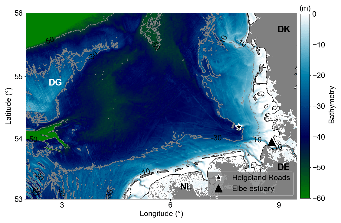
Figure 1 Bathymetry of the German Bight. Dotted–dashed, solid, and dashed grey lines are 10, 30, and 50 m isobaths, respectively. Areas with depths less than 5 m represented by white colour. The black star marks the location where the Helgoland Roads time series have been collected. The black triangle indicates the Elbe River estuary. DG refers to Dogger Bank, DE to Germany, DK to Denmark, and NL to the Netherlands.

2 Data and methods

2.1 Study area

The German Bight is a coastal area in the south-eastern North Sea bounded by the Netherlands (NL), Germany (DE), and Denmark (DK) (Fig. 1). The area defined in this work ranges from 2.5–9.25° N and 53–56° E. It extends from the Elbe estuary in the northwest, passes the Dogger Bank (DB), and has a maximum depth of about 50 m (Fig. 1). A 30 to 40 m deep funnel-like feature, defined by the deep Elbe valley, crosses the area in a diagonal direction from southeast to northwest (Stanev et al., 2014). The hydrodynamics of the region are very complex due to the interactions of riverine discharges, central North Sea water, Atlantic water (which flows into the region through the English Channel), and the tidal and atmospheric forcing (Becker et al., 1992; Kerimoglu et al., 2020).

The productivity in the German Bight is linked to its hydrographic conditions and bathymetric features (Emeis et al., 2015; Capuzzo et al., 2018). In regions where the depth is less than 20 m, the vertical concentration of Chl a is largely homogenized throughout the year, primarily due to the mixing effects of tidal currents and wind. However, in areas where the depth exceeds 20 m, the vertical Chl a concentration exhibits significant variability in terms of its extent, duration, and intensity (Schrum, 1997; Zhao et al., 2019). This variability is largely attributed to stratification and biogeochemical processes, such as the slow decomposition rates of organic matter (van Beusekom et al., 1999), which result in a distinct vertical Chl a distribution when compared to shallower regions (Zhao et al., 2019).

2.2 Chlorophyll a concentration remote sensing data

In this study, we downloaded the Copernicus Marine Service (CMS) GlobColour. daily interpolated cloud-free surface Chl a concentration product, ranging from January 1998 to December 2020 (CMEMS, 2023a). This product was available for download at the time of access on 20 October 2021 from https://resources.marine.copernicus.eu/, last access: 12 December 2021 under the product described as OCEANCOLOUR_ATL_CHL_L4_REP_OBSERVATIONS_009_ 098. This Chl a dataset was produced using multiple sensors (multi-sensor product), multiple Chl a algorithms, and a daily space–time interpolation scheme with a 1 km² spatial resolution (Garnesson et al., 2019).

2.3 Sea surface temperature, mixed-layer depth, and North Atlantic Oscillation (NAO)

Daily fields of sea surface temperature (SST) and mixed-layer depth (MLD) were obtained from CMS (https://data.marine.copernicus.eu/, last access: 20 April 2023), spanning from January 1998 to December 2020. The SST dataset (ESA SST CCI and C3S reprocessed sea surface temperature analyses; https://doi.org/10.48670/moi-00289, CMEMS, 2023b) contains gap-free maps of daily average SST at 0.05° horizontal grid resolution. It is a composition of satellite data from the Advanced Along-Track Scanning Radiometer (AATSR), Sea and Land Surface Temperature Radiometer (SLSTR), and the Advanced Very High Resolution Radiometer (AVHRR) (Lavergne et al., 2019; Merchant et al., 2019; Good et al., 2020).

Daily mixed-layer depth data (≈ 7 km horizontal resolution) are part of the Atlantic-European North West Shelf-Ocean Physics Reanalysis product (https://doi.org/10.48670/moi-00059, CMEMS, 2023c). The MLD was defined as the depth where the increase in density, compared to the density at 3 m depth, corresponds to a temperature change of 0.8° C (Kara et al., 2000; Tonani and Ascione, 2021).

The NAO winter index data were obtained from the Climate Analysis Section, National Center for Atmospheric Research (NCAR, Hurrell et al., 2023). It is calculated as the leading empirical orthogonal function of sea level pressure anomalies considering the gradient between the Icelandic Low and Azores High (Hurrell et al., 2003). The winter NAO index is the mean of the index for December, January, and February.

2.4 In situ data

In situ Chl a concentrations, measured with a high-performance liquid chromatography (HPLC) on a workday basis since 2004 at Helgoland Roads (see the black star in Fig. 1 for the data site) (Wiltshire et al., 2008), were used for the evaluation of the satellite-derived product. Helgoland Island is located in the German Bight approximately 60 km off the German coast, and since 1962 surface water samples have been collected at the Helgoland Roads site between the Helgoland and Düne islands (54° 11.3^′ N, 7° 54.0^′ E). The samples are representative of the whole water column due to the well-mixed conditions (Wiltshire et al., 2010). Helgoland Island is in a transition zone in the German Bight, influenced by offshore (higher-salinity) and coastal (lower-salinity) waters (Wiltshire et al., 2015).

2.5 Data pre-processing

As we were interested in long-term trends and variability, Chl a, SST, and MLD daily fields were monthly averaged values, which also avoids problems with missing spatial data. We computed monthly anomalies by subtracting the monthly mean absolute values from the climatological averages, which are the mean of monthly absolute values over the 1998 to 2020 period.

All spatial datasets were remapped to the grid of lowest spatial resolution (Table 1) using the bilinear method in the Climate Data Operators (CDO; Schulzweida, 2022). We excluded areas with bathymetry shallower than 5 m to circumvent dynamics related to intertidal zones. For analysis, coastal and offshore areas were defined by the isobaths of 30 m, following the description results obtained by the temporal mean and standard deviation, where areas with Chl a mean higher than 1 mg m⁻³ and standard deviation higher than 2 mg m⁻³ define coastal areas (see Fig. S1 in the Supplement). Consequently, the shallow Dogger Bank was considered in the offshore region.

The Chl a in situ data were monthly averaged values, and monthly anomalies were calculated. We extracted the nearest grid point from the Helgoland Roads location in the remote sensing gridded data (hereafter referred to as HRsat) and used monthly anomalies for comparison and validation of the GlobColour Chl a dataset.

Table 1 Description of the spatial resolution and source of the parameters used in this study.

2.6 Evaluation of satellite-derived Chl a data

We compared the HRsat monthly anomaly time series with the in situ (HPLC) Chl a monthly anomalies from the Helgoland Roads time series (HRTS) from 2004 to 2020. In this case, only the matching days were used for the calculation of the monthly anomalies in both HRsat and HRTS. Our primary focus was on trends and monthly variability to assess the degree of coherence between the in situ and remote sensing datasets. For the evaluation of trends, we applied the modified Mann–Kendall trend test (Kendall, 1975; Mann, 1945; Yue and Wang, 2004), and we made use of a boxplot for the variability assessment. The coefficient of correlation (r) and root-mean-squared error (RMSE) were computed to evaluate the goodness of fit between in situ and remote sensing data. Differences in distribution between Chl a in situ and remote sensing were verified by the two-sample Kolmogorov–Smirnov test (Massey, 1951).

2.7 Statistical methods

As a pre-analysis, we calculated temporal mean and standard deviation (SD) of the Chl a anomalies for the whole analysed period. Using the mean and SD, we computed the coefficient of variation (CV), calculated as $\mathrm{CV}=\frac{\mathrm{mean}}{\mathrm{SD}}\times \mathrm{100}$ (in %) (Morel et al., 2010). Additionally, we examined linear trends in Chl a anomaly fields. The significance of the linear trends was determined using a two-sided Wald test with t distribution. For more robust identification of significant positive and negative trends, we applied the modified Mann–Kendall trend test to the Chl a anomalies. This was done on a pixel-by-pixel basis using the Python “pyMannkendall” library (Hussain et al., 2019). The significance values are based on p values lower than 0.05 (95 % significance level). We calculated the probability density function to investigate the changes occurring in the distribution of Chl a anomalies, applying a Pettitt homogeneity test (Pettitt, 1979) to define a change point in Chl a anomalies.

We examined the relationship between the Chl a anomaly fields and SST and MLD anomalies (defined as Chl a|SST and Chl a|MLD, respectively) by applying linear correlations in the direct anomaly fields and in one-time-step-lagged (1-month-lagged) Chl a in relation to SST and MLD. For the analysis of dominant modes of Chl a variability and covariability with SST and MLD, we used maximum covariance analysis (MCA), a statistical technique that identifies prominent patterns of covariation (Bretherton et al., 1992) to maximize the covariability of associated parameters. MCA was designed to find patterns in two space–time datasets that explain the maximum fraction of the covariance between them. This can provide insight into the physical processes leading to the spatial and temporal variations exhibited in the fields being analysed. Given the known significance of SST and MLD forcing in inducing chlorophyll changes (de Mello et al., 2022), this technique is particularly suited for our purpose. In essence, MCA extracts the singular vectors of the cross-covariance matrix of two fields, in order of importance. These singular vectors, also referred as structures or modes of variability, are extracted. When MCA was calculated using only one field, such as the Chl a anomalies, we obtained the empirical orthogonal functions (EOFs), which represented the leading modes of Chl a variability. We utilized the Python package “xmca” (Rieger, 2021) to apply EOFs and MCA. For the EOF analysis, we used the monthly climatological Chl a concentrations and the Chl a anomalies, normalized during the analysis. For the MCA, the Chl a, SST and MLD anomalies were employed. To better interpret the MLD and EOF results, we used spectral analysis. The inflexion of the explained variance curve defined the limit for significant EOF modes.

3 Results

3.1 Evaluation of in situ and remote sensing chlorophyll a

Figure 2a illustrates the comparison of in situ and HRsat Chl a monthly anomaly time series. Both time series showed significant negative trends (in situ = −0.031 mg m⁻³ yr⁻¹; remote sensing = −0.025 mg m⁻³ yr⁻¹), evaluated by the modified Mann–Kendall trend test. While satellite observations accurately reproduced the intra- and inter-annual frequency, there was a discrepancy, with remote sensing tending to overestimate chlorophyll at low concentrations (Fig. 2b). In fact, satellite products tend to overestimate Chl a values when they are less than 1 mg m⁻³ (Alvera-Azcárate et al., 2021). When comparing the in situ and HRsat anomalies (Fig. 2a), we found a correlation coefficient (r) of 0.59 (p value <0.05) and root-mean-squared error (RMSE) of 1.09 mg m⁻³ (Fig. 2b). These values are in the range of values described in other works and considered acceptable for Case-2 waters (Silva et al., 2021; Pramlall et al., 2023), in which the remote sensing product is defined by other constituents besides chlorophyll, such as coloured dissolved organic matter and non-algal particles (Doerffer and Schiller, 2007).

Figure 2 Evaluation of GlobColour remote sensing surface Chl a compared to in situ data from Helgoland Roads. (a) Comparison of in situ (solid line) and remote sensing (dashed line) Chl a anomalies and respective linear trends (in mg m⁻³ yr⁻¹). (b) Scatter plot with linear correlation of the time series showed in (a). The correlation coefficient is 0.59, and the RMSE is 1.09 mg m⁻³.

In the boxplot (Fig. 3a) we observe that the in situ data have higher variability than the remote sensing data in April and May, months characterized by the phytoplankton spring bloom (Wiltshire et al., 2008). A rigorous assessment using the two-sample Kolmogorov–Smirnov test revealed no statistically significant differences between the anomaly distributions (p value = 0.83; Fig. 3b). The differences between in situ and remote sensing data were mitigated by using monthly mean anomalies. As a comparison, the evaluation using daily matchup Chl a anomalies time series gave values of r = 0.35 and RMSE = 2.64 mg m⁻³.

Figure 3 (a) Boxplots and (b) distributions of remote sensing (orange) and in situ (blue) monthly Chl a anomalies. The shaded areas in (b) are the superimposition of in situ and remote sensing bars.

3.2 General findings and Chl a overall trends

The average of Chl a (Fig. 4a) showed that higher concentrations (> 2 mg m⁻³) were generally found near the coast in areas with bathymetries less than approximately 30 m. This excludes the shallow region of Dogger Bank (Fig. 1). Areas with higher standard deviation (SD > 1 mg m⁻³) were also found in shallow areas, with a depth less than 30 m (Fig. 4b). The increased variability in these shallow areas is primarily due to larger seasonal differences compared to the offshore waters (see Amorim and Wiltshire et al., 2023, on temperature and seasonal variability comparisons for shallow and offshore sites). The standard deviation reflects the inter-pixel variability. Therefore, the coefficient of variation (CV) provided a measure of the spatial heterogeneity within the study area (Morel et al., 2010). The CV showed that 60 % of the studied area is between 40 % and 60 % (Fig. 4c), a medium term between stable and large fluctuations. Two areas with larger CVs are in the north, around the Dogger Bank and the Danish coastal zone, where there is a large bathymetry gradient; another area with high CV was found in the southern shallow waters of the Dutch coast, which is influenced by the water inflow from the English Channel. In the central region of the German Bight (GB), we have identified significant negative linear trends with values ranging around from −0.01 to −0.03 mg m⁻³ yr⁻¹ (Fig. 4d). In contrast, the southeastern corner of the study area, which is influenced by fresh water runoff from the Elbe river, exhibited positive significant linear trends (up to about 0.02 mg m⁻³ yr⁻¹).

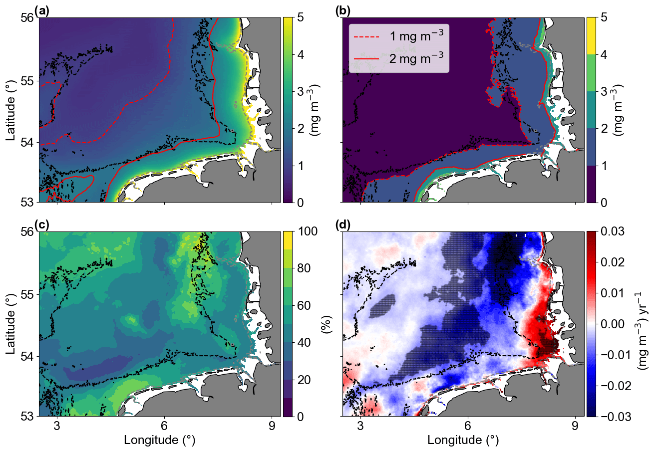
Figure 4 The (a) temporal mean and (b) standard deviation of chlorophyll a concentrations from January 1998 to December 2020. Solid and dashed red lines represent 1 and 2 mg m⁻³, respectively, and the dashed grey and black lines are the 10 and 30 m isobaths, respectively. (c) Coefficient of variation in percentage. (d) Trends of Chl a anomalies (mg m⁻³ yr⁻¹). The shaded areas are significant (p values < 0.05; two-sided Wald test with t distribution).

Since 1962 there has been a notable SST increase in the North Sea, a trend that persists to the present (1.3 °C from 1962 to 2019; Amorim and Wiltshire et al., 2023). Specifically, within the German Bight, the mean SST anomaly trend estimated by the locally weighted scatterplot smoothing method (LOWESS; Cleveland, 1979; Cheng et al., 2022) indicated an increase of 0.77° C from 1998 to 2020 (Fig. 5). This was further confirmed by the Mann–Kendall trend test, which showed a significant positive trend (p value < 0.001). This SST anomaly trend value is on the same order of magnitude as the one estimated by Mohamed et al. (2023) in the southern North Sea from 1982 to 2021 (0.33 ± 0.06 °C per decade). However, when it comes to the averaged MLD, no significant trend was observed.

The maximum and minimum SST anomalies were observed in July 2006 and April 2013, respectively. The maximum SST anomaly was 1.86 °C, and the minimum was −2.8 °C. Interestingly, after the observed minimum in 2013, a sharp increase to positive SST anomalies was observed, initiating a period with strong positive trends.

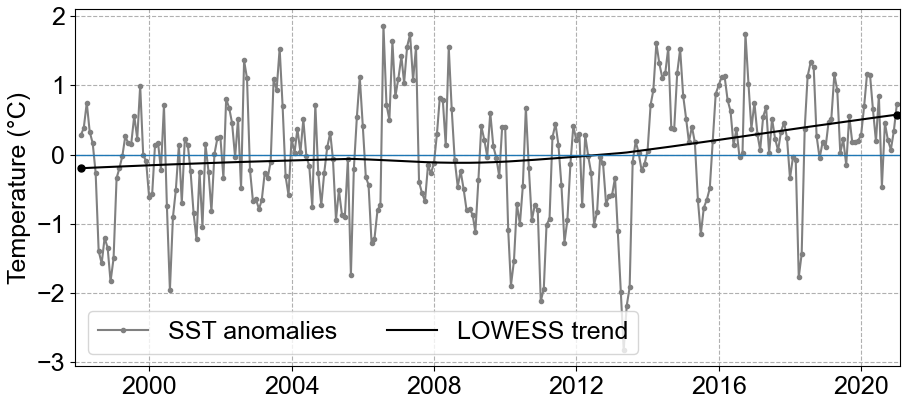
Figure 5 SST anomalies averaged for the whole German Bight (grey line) and the trend from 1998 to 2020 calculated by LOWESS (black line).

Figure 6 shows the trends of Chl a anomalies in the GB. A Mann–Kendall trend test showed that Chl a anomalies significantly decreased in 55 % of the analysed area (p<0.05). In the coastal area, mostly located in the southeastern corner of the study area, we found significant positive trends covering 6 % of the analysed area. In this region, there are available nutrients because of continued river input. Even with the turbid characteristic waters due to the river plume influence, light availability is not a limiting factor (Fichez et al., 1992; Kerimoglu et al., 2017).

Figure 6 Trend significance of Chl a anomalies computed with modified Mann–Kendall trend test. Pixels with p values < 0.05 are considered significant. The notation “dec. no sig.” indicates decreasing but not significant values, while “inc.no sig.” indicates increasing but not significant values.

Most of the central German Bight showed significantly negative trends. Amorim and Wiltshire et al. (2023) examined the winter mean NAO index and computed a positive trend. Naturally, the positive NAO phase is associated with strong and frequent westerly (W) and southwesterly (SW) winds during winter and spring. In addition, localized cyclonic systems over the British Isles can also generate such winds (see Rubinetti et al., 2023). As expected, there is a positive trend within the 21st century in the frequency of W and SW winds (Rubinetti et al., 2023). Due to the Ekman transport, SW and W winds suppress the spreading of coastal waters from the south of the German Bight offshore and intensify counter-clockwise wind-driven circulation in the German Bight (Schrum, 1997; Chegini et al., 2020). In addition, NAO in its positive phase characterizes strong Atlantic wind-driven inflow through the English Channel, increasing mean temperatures in the North Sea (Pingree, 2005). In the spatial SST average (Fig. 7), we can see a tongue with North Atlantic water temperature characteristics, i.e. warmer than the characteristic German Bight surface water. This means that negative and positive trends in Chl a offshore and at the coast, respectively, can partly be explained by the wind pattern and specifically by the increasing frequency of W and SW winds during winter and spring, which leads to limited offshore spreading of nutrient-rich coastal waters and increases the warm Atlantic water inflow into the North Sea.

Figure 7 Time-averaged sea surface temperature for the study area. The red line marks the 11.1 °C isotherm.

3.3 Seasonal chlorophyll a surface concentration

The monthly climatological means (Fig. 8) were characterized by decreasing concentrations from the coast towards offshore areas. It is possible to observe the intra-annual behaviour of Chl a, with a positive gradient from open waters to coast and an increase in Chl a in April and August. The months of April and May exhibited elevated chlorophyll concentrations, a result that aligned with existing literature on the spring blooms of diatoms (Wiltshire and Manly, 2004; Wiltshire et al., 2010; Neumann et al., 2021). A slight increase was observed in August, indicative of the late summer–autumn bloom of dinoflagellates (Yang et al., 2021).

Figure 8 Monthly averaged GlobColour Chl a from January 1998 to December 2020 (letters at the top right of each panel indicate the month). The Chl a monthly anomalies are calculated subtracting the monthly averaged Chl a from the absolute Chl a data.

Both coast and offshore areas were defined by a larger Chl a peak in April, describing the phytoplankton spring bloom. Higher variability was observed in the coastal area, and a smaller peak, representing the late summer–autumn bloom, was observed in August. Values below 2 mg m⁻³ were observed from November to February. The offshore area second peak was more perceptible compared to coastal areas, and it was observed in September/October (Fig. S3). The summer Chl a decrease was more accentuated in relation to the second peak in offshore areas, characterizing the period of lowest Chl a, below 1 mg m⁻³. The in situ HRTS acquired in the transitional zone of the German Bight, between coastal and offshore areas, aligned well with the spatial averages of Chl a remote sensing (Fig. S3).

The empirical orthogonal functions (EOFs) were applied to the climatological Chl a values and revealed a dominant seasonal variation. This variation was represented by the first and second modes, which together explained 88 % of the total variance in the annual cycle of Chl a in the region (Fig. 8). For interpretation, we made use of the variability signals in the spatial modes and structures (EOF) defined by the red and blue colours (positive and negative, respectively) together with the signal of the associated principal component (PC). The first spatial mode (EOF1) accounted for 53 % of the annual Chl a variability, exhibiting a positive signal across the entire German Bight. The first principal component (PC1) showed the two bloom signals, the spring bloom in April and the late summer bloom in September. Overall, mode 1 described the maximum positive Chl a variability during the spring bloom and, to a lesser extent, the late summer–autumn bloom (same signal in the spatial and PC temporal pattern), in contrast with winter and summer months, described by negative variability (opposite signals). The second spatial mode (EOF2) explained 35 % of the Chl a variability, dividing the GB into two regions based on the variability between cold and warm months. The coastal or transition region was defined by maximum negative variability during the winter months and positive variability during summer months according to the signals of EOF2 and PC2. In contrast, the offshore region showed negative variability during summer and positive variability during winter. This matched with the seasonal cycle of Chl a, with minimum Chl a months in coastal areas during winter and in the offshore region during summer.

Following the EOF mode 1 variability, we determined April and September to be the most contrasting months for explaining the positive Chl a variation in association with the environmental and biological or ecological drivers and winter and summer as the negative variability months.

3.4 Month of maximum chlorophyll a concentration

Considering the German Bight area analysed here, 96 % of the area had a maximum of climatological chlorophyll a observed in March, April, and May (20 %, 63 %, and 13 %, respectively), representing the main months of primary production and mainly related to diatom blooms (Wiltshire et al., 2008).

One interesting result for the remote sensing assessments was the month with maximum chlorophyll concentration (Fig. 9). Around the Helgoland Roads position, August was the month with maximum chlorophyll according to the remote sensing data. However, this is not consistent with the HRTS HPLC dataset. This might be an influence of the suspended matter dynamics (Fettweis et al., 2012) and/or the different pigmentation in phytoplankton species. Considering the two blooms occurring in the area, the spring bloom is characterized by dominant abundance of diatoms, while the late summer–autumn bloom also has a high abundance of dinoflagellates, which are more prone to develop in stratified periods and with different pigment compilations (Shang et al., 2014; van Leeuwen et al., 2015). There is a defined difference between the reflectance spectra of diatoms and dinoflagellates due to the distinct amounts of pigment types in each species (Shang et al., 2014) and such enhanced chlorophyll a could be associated with cellular motility and the ability to regulate position in the water column, resulting in enhanced near-surface aggregation of flagellated cells (Franks, 1992). The Dogger Bank area was characterized by an early maximum in March. This could be explained by the shallower bathymetry allowing for the earlier development of the spring bloom due to the abundant light availability and amount of nutrients available for the growth of phytoplankton (Moll, 1997; Los et al., 2008).

Figure 9 Month (colour bar from January to December) with maximum Chl a by pixel from the monthly climatology means of Chl a (Fig. 8; mg m⁻³). April (light grey) is the dominant month.

3.5 Chl a distribution before and after 2009

We examined the Chl a anomalies spatial averages for the months of March, April, and May over the 1998–2020 period to visually identify any potential increase or decrease in Chl a, assessing inter-annual variability in coastal and offshore areas. As the Mann–Kendall trend test did not point to any significant trends in the averaged Chl a anomalies, we analysed the changes in Chl a anomalies distribution, splitting the time series based on the April peak observed in 2008 for both coastal and offshore areas (Fig. 10). The peak in Chl a anomalies in 2008 was related to a positive peak in the North Atlantic Oscillation (NAO) index winter mean (Supplement Fig. S4). In 2010, a negative Chl a anomalies peak was observed in April and May in the offshore area and in May in the coastal area, coinciding with an negative peak in the NAO. After 2010, a positive NAO winter trend was observed. Considering these observations and the results obtained by the Pettitt homogeneity test, we defined two periods to analyse Chl a anomaly distribution, i.e. until 2009 and after 2009.

We calculated the probability density function of the two periods to investigate the changes occurring in the distribution of Chl a anomalies (Fig. 10). For the coastal area, March showed a shift from slightly normal to a bimodal distribution, with a small negative bias related to the mean. The bimodal distribution was still dominated by Chl a negative anomaly values but with a lower second peak in positive values, indicating years with positive Chl a anomalies. The offshore area distribution described an increase in variance and increase in positive anomaly values. These results could be the response of earlier spring blooms in the period 2010–2020 compared to the years before. April showed the highest variance change, decreasing from the first period (1998–2009) to the second period (2010–2020). The decrease in positive anomaly values was evident and it can be considered part of the negative trend observed in the German Bight, together with the shift in May, moving completely from positive to negative anomalies (Fig. 10). When associating the observed distribution changes with the observed overall trends, the period after 2010 is characterized by long phases of a positive NAO index. As already mentioned, the positive NAO phase is associated with the dominance of W and SW winds during winter and spring, increasing the inflow of Atlantic water in the German Bight and restricting the Elbe River discharge to coastal areas.

Figure 10 Probability density function estimated from 1998–2009 (blue) and 2010–2020 (orange) for the Chl a anomalies in March, April, and May in the coastal and offshore areas of the German Bight.

3.6 Dominant modes of non-seasonal chlorophyll a variability

EOF analysis was applied to examine the long-term non-seasonal variability in more detail. Recent studies have used this type of analysis on chlorophyll remote sensing and model simulation spatial data to detect the influence of environmental and oceanographic processes on phytoplankton biomass time–space variability (Daewel and Schrum, 2017; Alvera-Azcárate et al., 2021). Results of our EOF analyses showed that the first four modes accounted for 45 % of Chl a non-seasonal variability in the study area. The percent variance explained by each mode was 19.02 % (mode 1), 11.79 % (mode 2), 8.36 % (mode 3), and 5.54 % (mode 4). Figure 11 shows the spatial patterns for the EOF modes 1–4, which are associated with dominant long-term non-seasonal features since seasonal frequency cycles have been removed by the climatological monthly means subtraction procedure. The normalized amplitude time series (principal component, PC) corresponding to the spatial patterns (EOF) and the monthly means are shown in Fig. 12a–d and e–h, respectively. The PCs represent the time evolution of all pixels in the corresponding mode spatial pattern. If a pixel in the spatial pattern and its associated temporal amplitude have the same sign, it means a positive chlorophyll deviation for that pixel at that time in relation to the zero value in the spatial map. Conversely, when pixels in the spatial pattern and associated temporal amplitude show opposite signs, it means a negative deviation from zero. Therefore, pixels that show similar signs and values in the spatial pattern (Fig. 11) have similar behaviour in time and represent coherent features (Garcia and Garcia, 2008).

In terms of the spatial variability of Chl a, we show that there was distinct spatial and temporal variability in the German Bight concerning the modes of variability.

EOF1 showed the same signal for the whole German Bight, i.e. a decreasing variability from coast to offshore regions, and it is mostly related to inter-annual variability during spring blooms and positive peaks after the late summer–autumn bloom, as indicated by PC1. EOF2 split the area into offshore (northwest region) and transitional or coastal waters from southwest to northeast. EOF3 was characterized by a positive signal in the southwest region, possibly related to the English Channel inflow, bringing warmer waters to the German Bight. EOF4 can probably be related to stratification over a relatively long period mediated by the wind forcing and river forcing associated with Elbe and Weser freshwater discharges (Chegini et al., 2020). It is important to point that the modes or structures of variability contain information about the variability of the dataset that is not necessarily related directly to physical features. The interpretation of the EOF modes only aims to relate the data modes with physics (Olita et al., 2011). The temporal amplitudes associated with the spatial patterns are also subject to physical interpretation. To facilitate the interpretation of the PCs, we estimated the spectra of the main PCs (Fig. 12i–l).

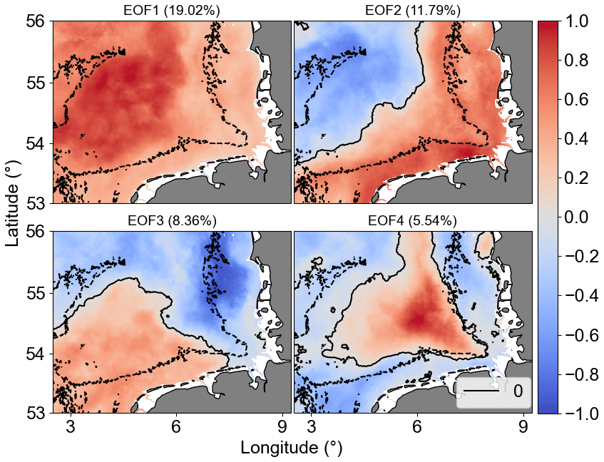
Figure 11 The first four Chl a anomaly EOF and PC modes. In EOF fields, the solid black line is the 0 amplitude contour, while the dashed black lines are the isobaths of 30 m. The amplitude values shown are scaled by the maximum value. The explained variability percentage for each mode is given in parentheses.

Figure 12 The first four Chl a anomaly PC modes. (a–d) The PC amplitudes (black) with six-point rolling means (solid red). (e–h) PC monthly means. (i–l) Spectral analysis of PC time series. The amplitude values are scaled by the maximum value. The explained variability percentage is given in parentheses. March–April (shaded green) and August–September (shaded pink) are highlighted in (e–h).

The spectral analysis of the Chl a anomalies' PC1 identified the highest peak over a period of 15 months and another high peak over an 11-month period, both related to the inter-annual variability of the spring bloom Chl a concentration in April. PC2 has peaks after 4, 6, and 12 months, linked to the intra-annual variability (Fig. 12j). In the averaged PCs, we can see that PC1 accounted for the variability of the two blooms, while PC2 was related to the decrease in Chl a during summer months happening mainly in deeper areas due to nutrient depletion during the spring blooms and zooplankton grazing. PC3 and PC4 together accounted for approximately 14 % of the variability and seemed to be characterized by extreme values occurring in sporadic periods due to the English Channel and Elbe River inflows, as observed in the EOFs.

3.7 Chlorophyll a, temperature, and mixed-layer depth relationships

Linear correlations revealed significant but not strong relationships between Chl a anomaly variability and SST or MLD anomalies in the study area (Fig. 13). For Chl a and SST correlations, the southern coastal area (along the Germany–Netherlands border) was characterized by significant positive correlation, while a patch of negative correlation was observed close to the Dogger Bank area. For Chl a and MLD, most offshore areas showed significant positive correlations, indicating that positive MLD anomalies were correlated to positive Chl a anomalies. The correlations between Chl a and MLD close to the coast and around isobaths of 30 m were negative. Lagged correlations between Chl a and the two parameters (SST and MLD) did not provide higher correlations, indicating that the Chl a variability possibly responds at timescales shorter or longer than a month. Focusing on the areas with significant correlation in Fig. 13, lagged Chl a and SST anomaly correlations were negative around the Dogger Bank, where bathymetry changes from around 50 m to shallower than 30 m in the bank area. The southern coastal area of the German Bight is described by positive correlations, a result not aligned with the Chl a overall trends, indicating an indirect effect of temperature on Chl a. The Chl a and MLD correlations are positive in most of the deeper parts of the GB, where higher Chl a values were found and connected with deeper MLD. In most of the areas shallower than 30 m, Chl a and MLD anomalies were negatively correlated.

Figure 13 Correlation maps of Chl a and SST (a, b) and Chl a and MLD (c, d). Panels (b) and (d) show 1-month-lagged correlations with Chl a. Warm colours are positive correlations, and cool colours are negative correlations. The dotted areas are significant (p values < 0.05; two-sided Wald test with t distribution).

Maximum covariance analysis (MCA) was carried out on Chl a anomalies and SST and MLD anomalies to identify spatial patterns. With this we hoped to explain as much as possible of the mean-squared temporal covariance between the two fields (Bretherton et al., 1992). MCA produces two sets of singular vectors along with a set of singular values. The relevant property of these singular vectors is that they maximize covariance (Von Storch and Zwiers, 2001; Martínez-López and Zavala-Hidalgo, 2009). The correlation coefficient between the “same mode” principal components of the two fields quantifies the strength of the coupled maximum covariance described by that mode (Martínez-López and Zavala-Hidalgo, 2009). This possibly tells us about how strongly the processes are connected or if there are other indirect processes involved and about the timescale coherence between the variables (Fukutome et al., 2003; Rieger et al., 2021)

Figure 14 Results of MCA showing the first co-varying mode between Chl a and SST anomalies. Panels (a) and (b) are the co-variability mode maps (Chl a: a; SST: b). Panels (c) and (d) are the temporal co-variability PC1 (c) and the corresponding spectra (d). PC1 is shown as rolling means of six points to better visualize the temporal co-variability of mode 1 between Chl a and SST anomalies.

The MCA Chl a|SST mode 1 (Fig. 14) presented positive anomalies covering the whole German Bight for SST, while Chl a showed negative anomalies in the deeper offshore area far from the coast and positive anomalies in the depths around 30 m and shallower. The largest negative Chl a anomalies in mode 1 were in areas surrounding the Dogger Bank, while the positive ones were in the coastal southern part of the German Bight. This pattern was already visible in the Chl a|SST anomaly correlation presented in Fig. 13. Mode 1 explained 45 % of the covariance between Chl a anomalies and SST anomalies, i.e. the non-seasonal variability. The result of MCA mode 1 was more or less what was observed in the spatial Chl a correlation, with positive correlation in offshore waters and negative correlation in the coastal areas. In the offshore region, we assume this is the role played by the critical depth theory (Sverdrup, 1953; Tian et al., 2011) and the weakening of turbulence after winter (Wiltshire et al., 2015). PC1 showed a significant weak correlation of 0.34, meaning weak coupling between the two PCs. The spectral analysis of PC1 did not show connected peaks, indicating that intra-annual variability in Chl a co-varies with lower frequencies of SST. The MCA Chl a|SST mode 2 anomalies explained much less (9.2 %) of this variability (not shown).

Figure 15 Results of MCA showing the first co-varying mode between Chl a and MLD anomalies. Panels (a) and (b) are the co-variability mode maps (Chl a: a; MLD: b). Panels (c) and (d) are the temporal co-variability PC1 (c) and the corresponding spectra (d). PC1 is shown as rolling means of six points to better visualize the temporal co-variability of mode 1 between Chl a and MLD anomalies.

The MCA mode 1 of MLD anomalies had the same signal in the majority of the analysed spatial domain, but Chl a mode 1 had a clear separation between coast and offshore regions (Fig. 15). MLD and SST work in opposite ways for these two regions. Even though mode 1 of Chl a and MLD anomalies accounted for approximately 23 % of covariance, less than Chl a |SST, the Chl a |MLD PC1 spectral analysis showed slightly higher coherence, with non-seasonal changes in MLD affecting Chl a in the same temporal scale.

4 Discussion and summary

The use of the Copernicus GlobColour chlorophyll a surface concentration allowed a comprehensive analysis of Chl a long-term trends and variability (23 years) in the German Bight. The evaluation of the GlobColour remote sensing dataset using a long HPLC Chl a time series from the Helgoland Roads site showed good agreement in trend and variability. The seasonal intra-annual variability in coastal and offshore areas of the GB was defined by two Chl a peaks, characterizing the spring and late summer–autumn phytoplankton blooms. Higher variability in coastal waters was observed between winter and bloom periods, while in offshore areas the higher variability was between summer and the bloom periods. The distribution of averaged coastal and offshore area Chl a before and after 2009 was characterized by clear changes in April and May Chl a anomalies, with a decrease in variance and the distribution peaks moving to negative values. Following the distribution changes, the overall trends in the German Bight were described by a large area in the centre of the GB with significant negative trends, with only a limited area close to the Elbe River influence showing significant positive trends. The dominant modes of the non-seasonal Chl a variability defined spatial and temporal components associated with inter-annual variability of Chl a during the bloom periods and a distinction between coastal and transitional areas and offshore areas. The English Channel and river inflows accounted for a small fraction of the explained Chl a variance. The covariability of Chl a anomalies with SST and MLD anomalies, assessed by maximum covariance analysis, showed higher covariability between Chl a and SST, but the spectral analysis and the lower PC correlation indicated distinct timescales of variability. In the case of Chl a and MLD covariability, the value was almost half of the one observed for SST but occurring over the same timescales. The low linear correlation between Chl a and SST could mean that there are indirect effects caused by temperature changes.

It is important to point out that the changes and variability in Chl a cannot be assumed to happen only due to SST or MLD because they occur as a combination of factors that can compensate or amplify each other (Xu et al., 2020). The relationship between SST and MLD together with the availability of light, nutrients, and turbidity controls most of the primary production variability in the German Bight. Changes in ocean surface temperature are associated with changes in other variables, including biological variables such as Chl a, primary productivity, species physiological responses, and species distributions (see Dunstan et al., 2018, for SST and Chl a covariability). Potentially, warming can either directly or indirectly affect the Chl a variability. Higher temperatures can alter the species physiological responses and species distributions (Dunstan et al., 2018). Wind patterns and freshwater discharge are impacted by climate change, and phytoplankton predation is enhanced by the increase in temperature due to the accelerated metabolism of zooplankton. The mechanism of influence becomes more complex as temperature modifies the physiology of species, species composition, river runoff, and other factors (van Beusekom and Diel-Christiansen, 2009; Capuzzo et al., 2018; Dunstan et al., 2018). Although there is a direct positive influence of increasing temperature, it is limited and can be outweighed by negative indirect effects and other factors, such as nutrient availability.

The German Bight, with its shallow bathymetry, does not behave like other marine regions, like the Arabian Sea and Sea of Japan, or like the oceanic gyres, where the changes in MLD are shown to be an important factor in Chl a changes mostly related to stratification and sea level anomaly (Prakash et al., 2012; Signorini et al., 2015; Park et al., 2020). A study in the Bohai Sea by Fu et al. (2016) identified an opposed result compared to our study, with positive trends in offshore areas and negative trends in coastal areas. Dunstan et al. (2018) described in their work how highly spatially heterogeneous the covariance of Chl a and SST is, pointing to the importance of regional studies and the complexity of the subject.

Capuzzo et al. (2018) pointed out that observed decrease in primary production in the North Sea from 1988 to 2013 is attributed to increasing temperature and a decrease in nutrients, as corroborated by the Desmit et al. (2020) analysis of the southern North Sea. In addition, van Beusekom and Diel-Christiansen (2009) identified that higher temperatures favour zooplankton growth and grazing during the spring blooms, decreasing the intensity of phytoplankton growth. Alvera-Azcárate et al. (2021) showed the heterogeneity of the North Sea, with areas presenting decreasing trends and others indicating slightly increasing trends of Chl a. A combination of factors is the most likely scenario under climate change for the primary production in the German Bight, but it is important to assess the individual consequences to better understand the whole situation.

5 Conclusions

The utilization of GlobColour chlorophyll a surface concentration enabled the identification of the primary modes of variability in the German Bight. Overall, the comparison between remote sensing and in situ data demonstrated consistent results in evaluating Chl a surface variability. Specifically, when comparing the in situ HRTS and remote sensing monthly anomalies, a correlation coefficient (r) of 0.59 and a root-mean-squared error (RMSE) of 1.09 mg m⁻³ were determined. The analysis of surface chlorophyll a concentration trends and variability was conducted in conjunction with anomalies in sea surface temperature and mixed-layer depth. For objective (i), spatial Chl a trends reveal a significant decrease in concentration in the central region of the German Bight over the past 23 years. In contrast, the near-coastal zone influenced by the Elbe River discharge exhibits a notable increase in chlorophyll a. Concurrently, a positive temperature trend is observed throughout the German Bight. It can be concluded that its direct positive influence on chlorophyll a concentration is limited and can be outweighed by negative indirect effects and other factors, such as nutrient availability and wind conditions. Over the last 23 years, a positive trend in the frequency of south-westerly and westerly winds during the winter and spring seasons has been observed, attributed to a prolonged positive NAO phase during the considered period. Such winds prevent the spreading of nutrient-rich coastal waters offshore from the southern German Bight and enhance the warm Atlantic water inflow into the central North Sea. This can in part explain the contrasting Chl a trends in offshore and inshore zones. For objective (ii), the EOF analyses of the chlorophyll a concentration showed the most variability in the intra-annual blooms (first mode) and the decrease in Chl a during summer in offshore areas and in winter months on the coast (mode 2), totalling around 88 % of explained seasonal variance. For the Chl a non-seasonal EOF results, the mode 1 (19 %) was defined by inter-annual variability, with a peak of energy in the spectrum at 11-month and 15-month cycle frequencies. This can be explained by the negative inter-annual variability in the spring blooms and positive variability after late summer–autumn blooms. The first four modes explained 45 % of the variability in total. The variability associated with the first four modes was defined by the division into offshore waters and transitional and coastal waters, intra-annual variability, English Channel inflow, and the presence of freshwater stratification. For objective (iii), the MCA analysis showed higher covariability between Chl a and SST anomalies than Chl a and MLD anomalies. The first mode of Chl a|SST represented 45 % of the covariability, while for Chl a|MLD, the first mode accounted for 23 % of the covariability. In the shallow German Bight, the impact of increasing temperatures is more important than stratification in the chlorophyll a variability. However, these temperature effects are mostly indirect, and temperature is an indicator of hydrographic changes in the German Bight. As a next step, we suggest performing an analysis of nutrients in the German Bight and relating possible changes with winds and stratification. A combination of remote sensing Chl a coupled with vertical in situ data would give even more insight into the 3D variability of Chl a in the German Bight.