Importance of tides and winds in influencing the nonstationary behaviour of coastal currents in offshore Singapore

Coastal currents significantly impact port activities, coastal landform morphodynamics, and ecosystem functioning. It is therefore necessary to understand the physical characteristics and natural variability of these currents within coastal settings. Traditional methods, such as harmonic analysis, assume stationarity of tide-driven currents and may thus not be applicable to systems modulated by variable nontidal inputs and processes. Here we deployed eight tilt current meters in shallow (< 5 m) coral reef environments in southern Singapore. Tilt current meters were positioned around the reefs at the main compass bearings to analyse the spatiotemporal variability of coastal currents in the frequency domain for 1 year (March 2018 to March 2019). Tidal motions were the primary mechanism of current flow on reefs and account for between 14 % and 45 % of total variance across all sites, with diurnal currents having either a similar or greater proportion of energy compared to semidiurnal currents. The relationship between currents and wind stress was then investigated across various frequencies. There is high correlation at low frequencies during the northeast monsoon, when the Madden–Julian Oscillation (MJO) is more active, thus generating currents that propagate either in phase or ahead of the MJO. At diurnal frequencies, the interaction between P₁ and K₁ results in a semi-annual cycle where currents are stronger during the monsoon seasons. This interaction could help to explain the seasonal variation in correlation as well as the K₁ amplitude, the latter of which could be further enhanced by the diurnal wind stress. The phase relationship between currents and wind stress is highly complex due to the variable bathymetry and could only be partially accounted for by the orientation of the coastlines relative to that of the wind. Given the importance of wind, we thus require longer time-series datasets to examine the role of atmospheric phenomena at greater timescales to improve our understanding of the variability of coastal currents.

1 Introduction

Nearshore currents in coastal waters have a profound impact on various applications. Coastal communities rely on port operations, fisheries, and recreational tourism for economic growth and sustenance and hence require robust infrastructure that is able to withstand strong currents (e.g. Klemas, 2011; Cervantes et al., 2015). Coastal currents also distribute nutrients, pollutants, and sediment either laterally or by vertical mixing, thereby influencing not only the morphodynamics of coastal landforms such as beaches, but also the composition and health of marine ecosystems such as coral reefs and mangroves (e.g. Covey and Barron, 1988; Klemas, 2011; Xue et al., 2012; Brunner and Lwiza, 2020; Sen Gupta et al., 2021). Therefore, it is imperative to improve our understanding of the physical characteristics of coastal currents and their natural variability across time and space.

Observed current velocities are the vector sum of the tidal and nontidal components. Nontidal currents are influenced by various factors, such as meteorological forcing and local bathymetry (e.g. Chen et al., 2014; Churchill et al., 2014). Tides and tidal currents can be expressed as a linear sum of sinusoidal tidal constituents, each with a known frequency (Foreman and Henry, 1989). Harmonic analysis (HA) is traditionally used to predict and fit the amplitude and phase of each tidal constituent to the observed tidal signal (e.g. Flinchem and Jay, 2000; Pawlowicz et al., 2002). For tidal currents, the lengths of semi-major and semi-minor axes (with the latter representing the direction of rotation), the phase, and the angle of inclination, collectively known as current ellipse parameters, are estimated. Cosoli et al. (2012) used HA on 2 years of surface current data in the northeastern Adriatic Sea and found tidal forcing to be weak, while correlation and coherence between wind forcing and nontidal currents were high. Churchill et al. (2014) also applied HA on Red Sea coastal currents over a 2-year period and likewise found tidal currents to be weak. Nevertheless, both studies acknowledged the possible contamination of tidal velocities due to diurnal wind stress. This is because one key assumption of HA is that tidal currents are stationary over the entire record length; i.e. the amplitude and phase of each tidal constituent stay constant over time (e.g. Flinchem and Jay, 2000). This assumption is often violated due to external forcing, such as variable wind stress, or other internal processes, such as river flow and tide–surge interaction (e.g. Horsburgh and Wilson, 2007). Moreover, as tides propagate into shallower waters near the coast, they undergo distortion, which may lead to the emergence of overtides, integer multiples of fundamental tidal harmonics which are typically used to describe nonlinear interactions such as friction and advection (e.g. Zhu et al., 2021).

Over the years, a variety of spectral techniques have emerged for studying nonstationary signals. Short-term harmonic analysis (STHA) involves conducting HA on short consecutive segments of the entire time series to provide moderate localisation of events involved in the modulation of tidal processes (Jay and Flinchem, 1995). Dusek et al. (2017) performed bimonthly HA on an 11-year record of estuarine currents in Tampa Bay, Florida, and found that tidal currents strengthen during periods of strong land–sea breeze and high freshwater discharge. However, STHA cannot resolve constituents with periods longer than the window length, nor can it capture the temporal variation in tidal constituents (Flinchem and Jay, 2000). In contrast, the wavelet transform uses a finite function with translation and scaling parameters, also known as the mother wavelet, to build a class of functions with a finite integrated squared value (e.g. Flinchem and Jay, 2000). Specifically, the continuous wavelet transform (CWT) uses an arbitrary number of these basis functions to convert the time series into two-dimensional plots of time and frequency, providing improved localisation of events (e.g. Jay and Flinchem, 1995; Torrence and Compo, 1998; Flinchem and Jay, 2000; Hoitink and Jay, 2016). However, the CWT is limited to extracting information on tidal species across different frequency bands instead of examining specific tidal constituents such as M₂ and K₁ due to the time–frequency trade-off governed by the Heisenberg uncertainty principle (Torrence and Compo, 1998; Flinchem and Jay, 2000). Additionally, to measure the cross-correlation between two CWTs, the magnitude-squared wavelet coherence (WC) is calculated (Grinsted et al., 2004).

The application of CWT is common in the study of estuarine dynamics. Jay and Flinchem (1995) revealed stronger semidiurnal and quarterdiurnal tidal signals during the generation of plume internal tides in the Columbia River estuary, though their relationships with physical mechanisms remain ambiguous. Analysing the CWT of currents has also yielded insights into how seasonal river discharge influences tidal damping and the modulation of shallow-water constituents in the Mahakam River in Indonesia (Sassi and Hoitink, 2013), the Yangtze River estuary in China (Guo et al., 2015), and the Guadalquivir River estuary in Spain (Losada et al., 2017). Zaytsev et al. (2010) employed both HA and a rotary-multiple filter technique, the equivalent of CWT, and found persistent intense anticlockwise rotary currents, presumably driven by anticlockwise sea breeze winds in the bay of La Paz, Mexico. Currents have a greater propensity for nonstationary interactions than water levels and should thus not be overlooked (Guo et al., 2015). However, the relationship between currents and other drivers remains unclear, with local wind forcing having a substantial impact on surface current variability (Ursella et al., 2006).

With this in mind, we aim to explore the nonstationary behaviour of coastal currents and their various drivers, with a focus on the Singapore Strait. The Singapore Strait links the South China Sea (SCS) and the Malacca Strait and is one of the busiest shipping routes in the world (e.g. Chen et al., 2005; Hasan et al., 2012). It has also undergone extensive development, such as land reclamation and shore protection work, which has majorly altered shoreline configuration and inevitably impacted local hydrodynamics. In the Singapore Strait, tidal asymmetry exists because tides transition from predominantly diurnal in the east to semidiurnal in the west (Chen et al., 2005; Tkalich et al., 2013); hence tides are semidiurnal, while currents are mostly diurnal (Van Maren and Gerritsen, 2012; Peng et al., 2023). The tidal asymmetry is further complicated by the complex bathymetry as many islands, such as rock outcrops and coral reefs, lie within the strait (Chen et al., 2005; Hasan et al., 2012). As depicted in Fig. 1, the Singapore Strait has a highly variable bathymetry of up to 100 m in depth, with deeper depths of up to 200 m recorded near Kusu Island. Additionally, the hydrodynamics are affected by local wind systems. Yearly, Singapore experiences two monsoon seasons with two inter-monsoons in between: the northeast (NE) monsoon from mid-November to March when northeasterly winds blow across the SCS and the southwest (SW) monsoon from mid-May to mid-September when wind circulation reverses (Van Maren and Gerritsen, 2012; Martin et al., 2022). The stronger and longer NE monsoon results in currents flowing net westward along the hydrodynamic pressure gradient from the SCS out to the Malacca Strait and Java Sea, only reversing direction during the SW monsoon (Chen et al., 2005; Van Maren and Gerritsen, 2012; Martin et al., 2022). The monsoons generally exhibit variability on different timescales from intraseasonal to interannual, with the former strongly influenced by the Madden–Julian Oscillation (MJO) and the latter by the El Niño–Southern Oscillation (ENSO) (Robertson et al., 2011).

Due to a lack of long-term observational records from Singapore, local hydrodynamics are typically modelled at coarse resolution and predicted using numerical models. Three-dimensional models have been used to simulate tidal currents in the Singapore Strait (e.g. Chen et al., 2005; Zhang, 2006) and have been further refined by expanding the grid boundaries (Hasan et al., 2012; Van Maren and Gerritsen, 2012) and incorporating multi-scale nesting to improve grid resolution (Hasan et al., 2016). These models were forced by major tidal constituents and did not include wind forcing due to heavy computational demands, thereby making the study of hydrodynamics in the Singapore Strait especially challenging. Nevertheless, such studies are crucial given their potentially significant implications for port operations, coastal sediment dynamics, and larval connectivity of marine ecosystems. In particular, sedimentation of fine-grained sediment is chronic within the Singapore Strait, and it influences the distribution and growth of coral reef communities. Here we focus on two coral reef platforms located within southern Singapore: Pulau Hantu (1.226247° N, 103.747049° E) and Kusu Island (1.225354° N, 103.860104° E) (Fig. 1). These fringing coral reefs are consistently subjected to high turbidity and sedimentation, as well as significant nearshore current velocities (Morgan et al., 2020). We used a 1-year time series of current velocity and direction data to achieve the following objectives: (1) analyse the general properties of currents and their ellipse parameters using harmonic analysis; (2) investigate the time-averaged properties of wind stress; (3) estimate the power spectral density (PSD) of currents in the Singapore Strait by partitioning the variance into four frequency bands and quantify the contribution of tides; (4) examine how the spectral properties of both currents and wind vary with time using CWT; and (5) evaluate their relationship using WC, complemented with the results of STHA. The structure of the paper is as follows: Sect. 2 covers the type of data collected and the methods employed to achieve the study objectives. The results of the study are described and discussed in Sects. 3 and 4 respectively. Lastly, conclusions are given in Sect. 5.

Figure 1 (a) A map of the Southeast Asia region (Amante and Eakins, 2009), with Singapore indicated by the black rectangle. (b) A zoomed-in map of Singapore with the location of our study areas, Pulau Hantu and Kusu Island, in the southern coast of Singapore (indicated by the red squares). The background colour represents the bathymetry (GEBCO Bathymetric Compilation Group, 2023; Navionics, 2023). (c) A zoomed-in map of Pulau Hantu with the four study sites where the TCMs are deployed, marked by yellow circles and labelled according to their compass bearings, and (d) likewise for Kusu Island.

2 Data and methods

2.1 Data collection

The bathymetry data of Singapore shown in Fig. 1 have a 25 m resolution and were compiled from several sources: the Hydrographic and Nautical Charts from Navionics WebApp (Navionics, 2023), the General Bathymetric Chart of the Oceans at a 15 arcsec resolution (GEBCO Bathymetric Compilation Group, 2023), the 2019 version of the 10 m digital terrain model (DTM) map of Singapore (Victor Khoo, Singapore Land Authority, personal communication, 2019), and the 30 m Shuttle Radar Topography Mission data (NASA JPL, 2013). The land boundaries of Malaysia and Indonesia were obtained from Hijmans and the University of California (2015) and the Humanitarian Data Exchange (2024) respectively.

At Pulau Hantu and Kusu Island, we deployed four tilt current meters (TCMs; TCM-1 Lowell Instruments) following the main compass axes of the reefs (north, south, east, and west) (Fig. 1). TCMs operate by the drag-tilt principle, in which the meter tilts in the direction of the drag of the fluid. To minimise the effects of vortex eddies, turbulence, and waves, the TCM was configured to record data at 8 Hz for 15 s (i.e. 160 samples) per minute, and the data are burst averaged over each minute (Lowell et al., 2015). The accuracy specifications of TCMs for speed and direction are 3 cm s⁻¹ + 3 % of reading and 5° for current speeds exceeding 5 cm s⁻¹ respectively. We collected data on speed, direction, and zonal (u) and meridional (v) velocities at a 10 min sampling interval at a shallow depth of ∼ 3 m from March 2018 to March 2019, except at Hantu North where data were collected until December 2018 due to instrument malfunction. From the 51 000 data observations, there were eight and seven consecutive missing data points in Hantu West and Kusu South respectively. Since data need to be continuous for wavelet analysis, we interpolated the missing data using a moving median with a window length of 2 h.

To examine the role of local winds, we obtained dynamically downscaled hourly zonal and meridional wind velocity data from the Tropical Marine Science Institute in Singapore. Dynamical downscaling was performed using the Weather Research and Forecasting (WRF) model version 4.4.1 (Skamarock et al., 2019). The WRF model was set up with a horizontal grid of 10 km resolution covering Southeast Asia and centred at a point with coordinates 8.5° N and 115° E, and it was then forced by ERA5 atmospheric reanalysis data, whose horizontal resolution is 0.25° × 0.25° or about 31 km (Hersbach et al., 2020). We extracted the wind data from the grid points closest to both islands and used the drag coefficients from Large and Pond (1981) to derive wind stress from wind velocities at 10 m reference height.

2.2 Analysis methods

We first performed principal component analysis (PCA) to resolve both currents and wind stress, initially expressed as eastward and northward vectors, into uncorrelated orthogonal components with their mean value subtracted. PCA is useful for analysing highly directional variables such as coastal currents, which generally flow parallel to the coastline. Therefore, its alongshore and cross-shore current can be defined by the major and minor axis component respectively, the former of which accounts for most of the total variance (Thomson and Emery, 2014). We then performed harmonic analysis on currents at each site over the entire observation period using the MATLAB UTide package (Codiga, 2011) to extract the current ellipse parameters of major tidal constituents. Additionally, we calculated the hourly and monthly wind stress averages of both Pulau Hantu and Kusu Island to examine the variation across different periods.

Using the MATLAB toolbox jLab (Lilly, 2019), we chose a time-bandwidth product of 3 and 13 Slepian tapers to obtain multi-taper PSD estimates of currents and wind. This method provides a smoother estimate of the spectrum than the traditional Fourier transform as the spectrum is an average of multiple independent spectrum estimates that are generated from the same sample, thereby minimising spectral leakage (Percival and Walden, 1993). The sampling rate for both currents and wind stress converts to a Nyquist frequency of 72 cycles per day (cpd) and 12 cpd respectively. We visually inspected the spectra for any peaks and gaps before partitioning the variance into four frequency bands: low frequency, f < 0.72 cpd; diurnal, f = 0.72–1.5 cpd; semidiurnal, f = 1.5–2.3 cpd; and high frequency, f > 2.3 cpd. Hereafter, diurnal and semidiurnal frequencies are collectively referred to as tidal frequencies. We then quantified the variance by integrating the spectrum over each frequency band via rectangle approximation and expressed the relative contribution as a percentage of the total variance. The 95 % confidence intervals for spectral estimates were calculated assuming a χ² distribution of variance.

Wavelet analysis was done with the MATLAB toolbox cross wavelet and wavelet coherence (Grinsted, 2023). To analyse the time series at different periods or frequencies, the wavelet is scaled accordingly and translated in time. We selected the Morlet wavelet as it is optimal for processing tidal signals, 12 scales per octave, and a dimensionless frequency of 6 to provide a good balance between time and frequency resolution (Torrence and Compo, 1998; Grinsted et al., 2004). The wavelet power is normalised by the variance of the time series, and the cone of influence (COI) demarcates the area where edge effects cannot be ignored (Grinsted et al., 2004). Edge effects typically arise when the wavelet is stretched and located near the start and end of the data because it extends outside the boundary of the time series. Therefore, information that lies outside the COI should be treated with caution.

Finally, we used WC to examine the strength and phase of the localised correlation between currents and wind stress. The arrows in WC analysis represent the relative phase or the time lag between both variables, with the level of statistical significance estimated using Monte Carlo methods (Grinsted et al., 2004). The time lag at a specific period is calculated as the phase angle divided by 2π times the period and requires careful interpretation. For instance, arrows pointing to the left represent an anti-phase relationship, which could either indicate negative correlation or one variable leading the other by half the period. An in-phase relationship means that the relative phase is 0° with arrows pointing to the right. We complemented WC with STHA to observe any similar trends. We ran STHA through the MATLAB toolbox UTide (Codiga, 2011) using a 60 d window and moved with a time step of 1 d to provide seasonal resolution while maintaining result accuracy. A bimonthly window also resolves 35 tidal constituents, including those with longer periods up to monthly such as M_m, and in this case constituents with similar frequencies N₂ and M₂.

3 Results

3.1 General characteristics of currents

From the PCA results, the alongshore current accounts for 67 % to 87 % of current variance in most study sites but only 54 % in Hantu West (Table 1). This could be attributed to the slightly concave nature of the coastline of Hantu West, and hence flow is not strictly rectilinear. Mean and maximum current speeds across the time series were also calculated for each site. Within the time domain, the mean speed of currents at the Pulau Hantu sites ranged from 9.3–19.6 cm s⁻¹, with maximum speeds of up to 119.8 cm s⁻¹ (Table 1, Fig. 2). Currents at the Kusu Island sites are generally weaker throughout the duration of the study, with mean speeds ranging from 6.7–14.7 cm s⁻¹ (Table 1). Sites situated at the east and west of both islands experience higher mean speeds of 11.6–19.6 cm s⁻¹, as compared to the north and south sites where mean speeds are weaker and do not exceed 10 cm s⁻¹ (Fig. 2). During the spring tides, current speeds more than quadrupled from about 20 cm s⁻¹ to about 100 cm s⁻¹ consistently at both Hantu East and Hantu West. However, at Hantu North, Hantu South, and Kusu West, the increase in speed is less consistent, also reaching up to about 100 cm s⁻¹, but only during five periods of spring tide every month during the monsoon seasons from May to September and from December to March. At Kusu South, currents exceed 40 cm s⁻¹ only in March–April 2018 and remain weak over time. Kusu East and Kusu North exhibit consistent temporal variation, with the former recording slightly greater speeds during the NE monsoon.

Table 1 Properties of the principal components of currents.

Figure 2 Current speeds over time at (a) Hantu North, (b) Kusu North, (c) Hantu South, (d) Kusu South, (e) Hantu East, (f) Kusu East, (g) Hantu West, and (h) Kusu West.

Current ellipses for the major tidal constituents were calculated using harmonic analysis and presented in Fig. 3. The amplitudes of the ellipses are greater at the east and west sites of both Pulau Hantu and Kusu Island, which meant stronger currents in those areas, while the amplitudes at Kusu South are the lowest. The eccentricity of the ellipses, which can be loosely defined as the ratio of the semi-minor-axis length to the semi-major-axis length, is very low across most sites and thus indicates a rectilinear flow along the coastlines, while the ellipses at Hantu West are slightly rotund. Such results align well with the earlier analysis. In addition, the diurnal tidal currents are generally more dominant, as seen from the larger K₁ and O₁ amplitudes, while the semidiurnal M₂ currents are only strong in Hantu East and Hantu West. M₂ currents are much stronger than S₂ currents, and the amplitudes of P₁ currents are very small compared to the main diurnal constituents. It should be emphasised that the current ellipses, while useful for displaying the strength and orientation of currents, do not include any information about the nonstationary behaviour of currents and should thus be complemented with the extra techniques outlined in the previous section.

Figure 3 Tidal current ellipses for M₂ (a, b), S₂ (c, d), K₁ (e, f), O₁ (g, h), and P₁ (i, j) at all study sites in Pulau Hantu (left column) and Kusu Island (right column). Ellipses are depicted in red if they show an anticlockwise movement. Wind roses for wind stress from March 2018 to March 2019 at (a) Pulau Hantu and (b) Kusu Island.

3.2 General characteristics of wind stress

The major axis wind stress over Pulau Hantu and Kusu Island accounts for 61 % and 77 % of the wind variance respectively and blows predominantly to the southeast from the SCS, with Kusu Island recording stronger winds (Table 2). These winds strengthen during December to March and are thus representative of the NE monsoon. In contrast, the wind direction of minor axis winds is directed north-westward, and these winds become stronger from June to September, thereby coinciding with the SW monsoon. The wind rose for both Pulau Hantu and Kusu Island provides a good visualisation of the strength and directionality of the winds (Fig. 3).

Table 2 Properties of the principal components of wind stress.

Wind stress was averaged for both Pulau Hantu and Kusu Island over each hour of the day (Fig. 4a). The average wind stress along both principal components is diurnal and asymmetric, characteristic of the land–sea breeze circulation in Singapore. The northeast and northwest directions are taken to be positive for the major and minor axes respectively (Table 1). During the day, averaged wind stress is directed north and reverses in direction at night, with maximum magnitudes of the major axis winds occurring at about 13:00 and 20:00 local time (LT) at Pulau Hantu. The maximum major axis wind stress during the day at Kusu Island occurs slightly earlier, at about 11:00 LT. Owing to differential heating between the land and sea, the sea breeze blowing northward from the Singapore Strait during daytime is usually stronger than the land breeze coming from the Malay Peninsula late at night (Li et al., 2016). Interestingly, the diurnal pattern is more pronounced from about June to November, which comprises the SW monsoon and the following inter-monsoon period, where the averaged wind stress increases in strength and is directed northward as seen from the monthly-averaged plot (Fig. 4b). Likewise, we can infer that the daily variation in averaged wind stress during the NE monsoon and the following inter-monsoon period, from about December to April, is a predominantly southward orientation that is most intense at night (Fig. 4b).

Figure 4 Wind stress of Pulau Hantu and Kusu Island with their respective principal axes, averaged over (a) the hour of the day and (b) the month of the year.

3.3 Power spectral density

We calculated the PSD to partition the variance into frequency bands and quantified them for both alongshore and cross-shore currents. Here we can observe that spectral peaks are most prominent at tidal frequencies, with diurnal currents being slightly stronger than semidiurnal currents (Fig. 5). The spectra yield two distinct peaks within the diurnal band, which correspond to the major diurnal tidal constituents K₁ (1.0032 cpd) and O₁ (0.9288 cpd). Higher-frequency signals from the third diurnal band to the eighth diurnal band are also discernible, though not as strong as currents oscillating at tidal frequencies. Meanwhile, only the fortnightly signal is significant within the low-frequency band, which could represent the lunisolar synodic fortnightly tidal constituent MS_f. The MS_f constituent illustrates spring–neap variations caused by quadratic nonlinear interactions of the M₂ and S₂ tidal constituents (Hoitink and Jay, 2016). Wind stress spectra also show the presence of a strong land–sea breeze, evidenced by the sharp and narrow peaks occurring at periods of about 24 and 12 h, with the latter being less pronounced.

Figure 5 Power spectral density estimates of both major axis and minor axis wind stress in (a) Pulau Hantu and (b) Kusu Island, with units of square pascals per cycle per day, as well as those of both alongshore and cross-shore currents recorded at (c) Hantu North, (d) Kusu North, (e) Hantu South, (f) Kusu South, (g) Hantu East, (h) Kusu East, (i) Hantu West, and (j) Kusu West, with units of square centimetres per square second per cycle per day. The shading indicates the 95 % confidence level for the major axis wind stress and alongshore currents. The vertical dashed black lines loosely represent (from left) the fortnightly (D_f) frequency bands shown only in the currents plots and diurnal (D₁) and semidiurnal (D₂) frequency bands.

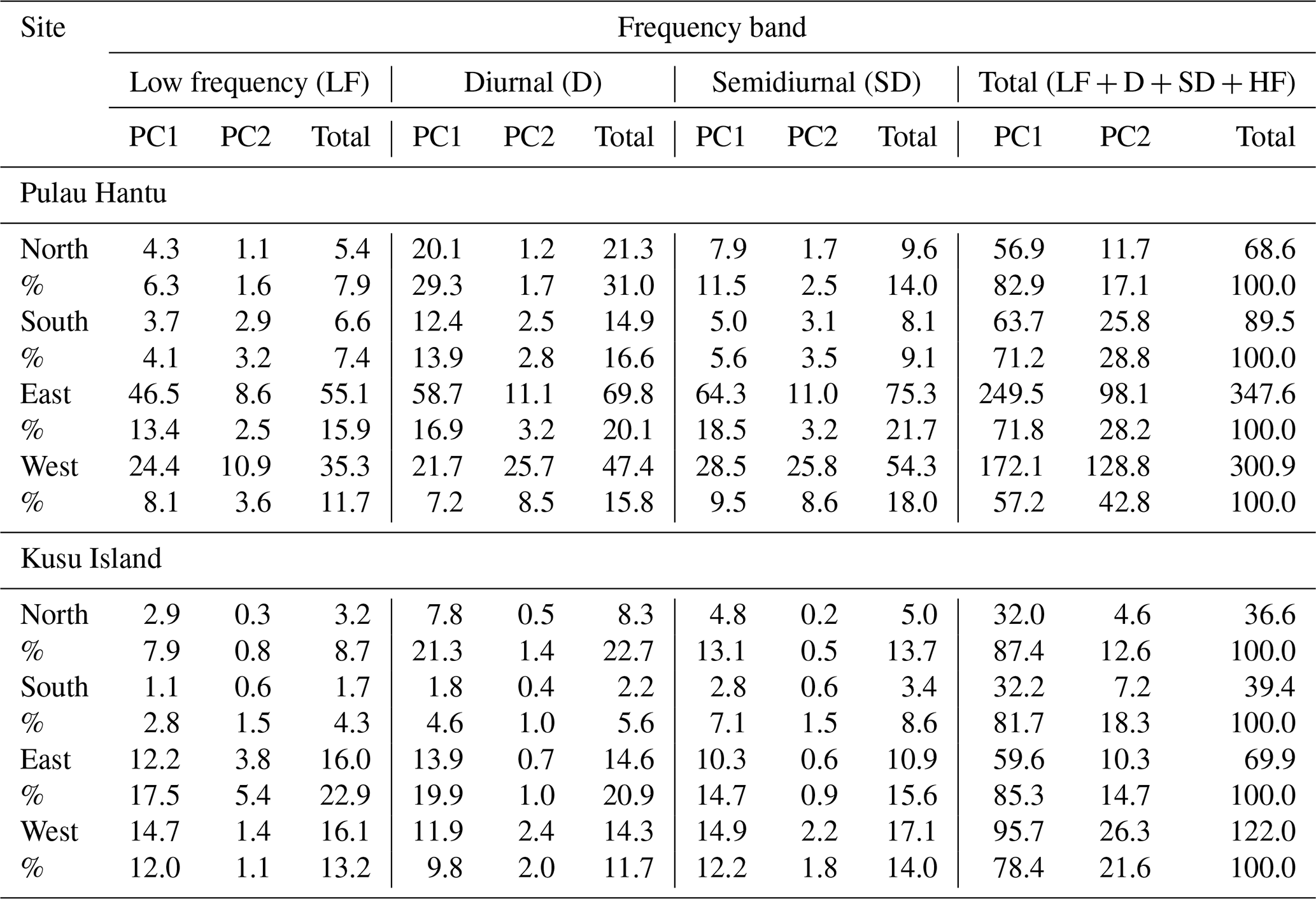
Table 3 presents the total velocity variance, which is the sum of the variances of low-frequency (LF), diurnal (D), semidiurnal (SD), and high-frequency (HF) bands, and the variances of LF, D, and SD motions. The variance of alongshore and cross-shore currents, denoted by PC1 and PC2 respectively, is also shown for each frequency band. The total percentage variance of PC1 and PC2 currents is similar to the PCA results shown in Table 1. Tidal frequencies are responsible for about 26 %–45 % and 14 %–36 % of the total current variance across all sites in Pulau Hantu and Kusu Island respectively, with the spectral energy of diurnal currents being at least 1.3 times higher than semidiurnal currents in Hantu North, Hantu South, Kusu North, and Kusu East (Table 3).

Table 3 Variance (in cm² s⁻²) of the filtered currents obtained from PSD. The variance for each frequency band is calculated by integrating the spectrum using rectangle approximation, with the relative contribution expressed as a percentage of the total variance. The variance of high-frequency currents is not shown here.

3.4 Continuous wavelet transform of currents and wind stress

The CWT of alongshore and cross-shore currents at all study sites shows that the diurnal and fortnightly signals are the strongest and statistically significant (Fig. 6 and Fig. S1 in the Supplement). In addition, energetic semidiurnal and monthly signals are also present. Strong alongshore currents at tidal frequencies occur about twice a month, which incidentally coincided with the spring–neap tidal cycle. The presence of statistically significant regions in Hantu West is better observed in the CWT of its cross-shore currents (Fig. S1), where there is minimal spectral leakage and currents are the strongest at tidal and fortnightly frequencies. High-frequency oscillations are also present year-round, highlighting the chaotic nature of currents flowing near the coasts. The wavelet power is generally negligible between the period of 1 to 8 d. In addition, strong low-frequency currents are detected at a periodicity of about 32 d (Figs. 5 and S1), which likely indicates the presence of intraseasonal variability.

Nonstationary behaviour of currents is clearly exhibited, as the wavelet power across frequency bands shows significant temporal variation. Alongshore currents are unusually weak during the inter-monsoon period from September to October in Hantu East, Hantu South, and Kusu West, with Kusu West showing the greatest contrast (Fig. 6). At Kusu East and Kusu North, diurnal currents seem to intensify when the NE monsoon begins in December, which contrasts with Kusu South where currents at tidal frequencies are heavily attenuated from November onwards (Fig. 6).

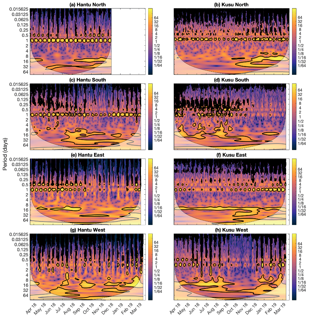
Figure 6 CWT of alongshore currents at (a) Hantu North, (b) Kusu North, (c) Hantu South, (d) Kusu South, (e) Hantu East, (f) Kusu East, (g) Hantu West, and (h) Kusu West. The thick black contour encompasses significant regions against red noise (p < 0.05), and the cone of influence (COI) is shown as a lighter shade where edge effects cannot be ignored. The wavelet power is log ₂(A² v⁻¹), where A is the wavelet amplitude, and v is the variance of the entire signal.

The CWT of wind stress presents powerful and statistically significant oscillations at the diurnal and monthly frequencies (Fig. 7). Diurnal wind stress is the strongest during the NE monsoon from December to March. The minor axis diurnal wind stress at Pulau Hantu, while not as strong during the NE monsoon, recorded considerable strength in the months from June to October, the period when the SW monsoon regime is dominant. Similar to the CWT of currents, the low-frequency winds are the strongest in periods of about 32 d from December to February for Pulau Hantu and from April to October for Kusu Island, which suggests periods of strong MJO activity.

Figure 7 CWT of wind stress at (a) Pulau Hantu major axis, (b) Pulau Hantu minor axis, (c) Kusu Island major axis, and (d) Kusu Island minor axis.

3.5 Wavelet coherence between currents and wind stress, as well as STHA of currents

The WC between both alongshore currents (Fig. 8) and cross-shore currents (Fig. S2) and major axis wind stress reveal a strong correlation over a broad range of frequencies, with the low-frequency and diurnal frequency bands being the most significant. The arrows represent the phase relationship between both variables; arrows pointing upwards with respect to the phase indicate that currents lead wind stress and vice versa.

At periods of 32 d or longer, correlation from September onwards is high, significant, and largely in phase at most sites. This suggests that the MJO plays a significant role in modulating the intraseasonal variability of coastal currents. At Kusu North and Kusu South, the phase difference of 30° indicates that the currents lead the winds by a few days. However, at Hantu North and Kusu East, the relative phase is approximately 90–120° pointing down, which means that strong currents occur about 1 to 2 weeks later.

At the diurnal frequency band, correlation was generally significant, albeit rather sporadically, during the monsoon seasons for most sites. This suggests that nontidal processes, such as wind stress, introduce nontidal energy at tidal frequencies (Pugh, 1987). In addition, the relative phase relationship has considerable temporal and spatial variability. Correlation is weak and close to zero during the inter-monsoon from September to November, albeit with short periods of high correlation in between (Figs. 8 and S2). During the SW monsoon from June to September, correlation between the major axis wind stress and alongshore currents is high and approximately in phase at Hantu East, Hantu South, Kusu East, and Kusu North (Fig. 8), with a phase angle at Kusu East of about 0–90° pointing down. This corresponds to wind stress leading currents by up to 6 h. In contrast, the correlation at Hantu North is almost anti-phase. Considering the NE monsoon, statistically significant regions are observed in Hantu East, Hantu South, Kusu East, Kusu North, and Kusu West. The correlation is approximately in-phase at Kusu West and anti-phase at Hantu East and Kusu East, while the phase relationship at Hantu South and Kusu North is highly variable with the phase angle fluctuating wildly from 0–270° with respect to the phase. As such, it is not immediately clear whether the currents or wind stress is the leading variable.

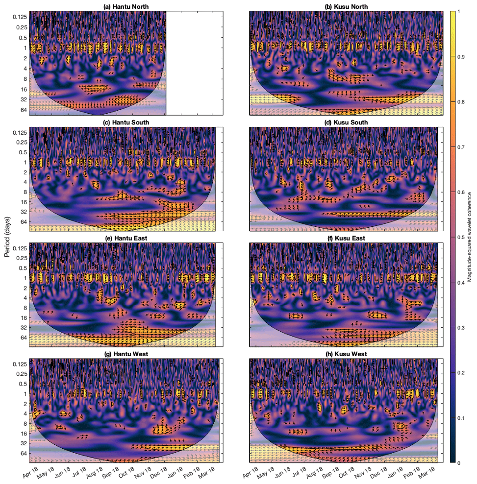
Figure 8 Wavelet coherence between alongshore currents and major axis wind stress at (a) Hantu North, (b) Kusu North, (c) Hantu South, (d) Kusu South, (e) Hantu East, (f) Kusu East, (g) Hantu West, and (h) Kusu West. The black contours indicate significant regions and the cone of influence (COI). The area that lies outside the COI has a lighter shade, and information in this area should be treated with caution. The arrows represent the relative phase relationship, with right- and left-pointing arrows indicating in-phase and anti-phase relationships respectively, and winds leading currents by 90° pointing down.

We presented the semi-major-axis amplitude of four main tidal constituents K₁ (Fig. 9), O₁, M₂, and S₂ (Figs. S3–S5 respectively). Though the amplitudes of most major tidal constituents are generally large, they do not seem to exhibit any trend. However, except for Kusu South where currents are generally very weak, the amplitude of the K₁ tidal constituent appeared to vary semi-annually and ranges from about 1 to 18 cm s⁻¹ during the monsoon seasons. In Pulau Hantu, the K₁ amplitude is generally greater than that in Kusu Island, which is not surprising since currents in Pulau Hantu are generally stronger. This suggests that diurnal wind forcing amplified during the monsoon seasons could result in a corresponding increase in the K₁ amplitude of currents.

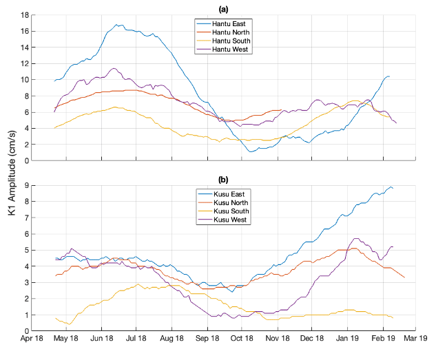
Figure 9 K₁ tidal amplitudes of all sites in (a) Pulau Hantu and (b) Kusu Island, derived from STHA.

4 Discussion

The high correlation displayed in the coherence analyses indicates the significance of wind forcing in driving currents at various timescales. Low-frequency winds in the tropics are dominated by the MJO, a period of 30–90 d defined by the eastward propagation of deep atmospheric convection and anomalous rainfall in the tropical Pacific (Madden and Julian, 1971; Zhang, 2005). Hu et al. (2023) discovered that as the MJO crossed through the Maritime Continent during the winter months from November to March, there was an anomalous eastward subsurface warm current in the Timor Sea propagating ahead of the MJO convection centre due to a deeper thermocline excited by the wind field anomalies. Likewise, the generation of MJO convection in the later months of the year creates persistently strong coastal currents in Pulau Hantu and Kusu Island that could help to sustain the MJO propagation.

Diurnal currents are stronger than semidiurnal currents (Fig. 7) due to the presence of an amphidromic point for the main diurnal constituents in the Singapore Strait (Pugh, 1987). Van Maren and Gerritsen (2012) further deduced that the K₁ tide is a standing wave as it propagates from the SCS and reflects off the Sumatra coast, generating high velocities in the Singapore Strait that are predominantly diurnal despite Singapore experiencing a semidiurnal tidal regime. Additionally, only the K₁ currents exhibit semi-annual variation, with amplitudes increasing during the monsoon seasons (Fig. 9). It is not uncommon to observe seasonal modulation in tides and tidal currents, particularly in shallow waters where there are seasonal changes in stratification. During the summer when there is less mixing in the water column, there is reduced vertical eddy viscosity and energy loss, leading to higher tidal amplitudes and hence stronger currents (Müller, 2012). For instance, the amplitude of the M₂ tide and tidal currents are larger during the summer in the East China and Yellow seas (Kang et al., 2002) and the Bohai Sea (Wang et al., 2020). However, Singapore's water column is generally fully mixed with minor stratification during neap tides (Hasan et al., 2013). We then postulated that other mechanisms, such as interaction between tidal constituents and meteorological forcing, are responsible for the seasonal modulation of K₁ currents. For example, seasonal tidal variations correspond to the western North Pacific monsoon index in Southeast Asia (Devlin et al., 2018) and to ENSO in the Solomon Islands (Devlin et al., 2014).

We used the results of harmonic analysis to reconstruct alongshore current velocities using only K₁ and P₁ constituents. Although the amplitude of P₁ is much smaller than K₁ (Fig. 3), their interaction results in a pronounced semi-annual variation of about 183 d, the inverse of the difference in their frequencies (Fig. 10). This phenomenon is also observed in diurnal tides in the southern SCS, where diurnal internal tides are more energetic during the summer and winter months, when monsoonal winds are incidentally stronger (Shang et al., 2015). The modulation of K₁ and P₁ thus enhances diurnal currents during the monsoon seasons when wind stress is also greater. This could help to elucidate the seasonal variation in the K₁ amplitude (Fig. 9) and its correlation with diurnal wind stress (Fig. 8). Moreover, the seasonality could also be augmented by potential resonant dynamics as the dominant frequency of diurnal wind stress and the K₁ frequency are largely similar, thereby establishing the role of wind stress in introducing nontidal energy at the K₁ frequency. This finding corroborates with prior results presented by Álvarez et al. (2003) and Dusek et al. (2017), both of whom concluded that changes in the sea breeze wind stress are responsible for the seasonal variations in the K₁ amplitude of estuarine tidal currents in Cádiz Bay, Spain, and Tampa Bay, Florida, respectively.

Figure 10 Reconstructed alongshore current velocities using only P₁ and K₁ tidal constituents.

The phase relationship between currents and winds also exhibits nonstationary behaviour (Fig. 8). During the SW monsoon, the effect of diurnal wind forcing at Hantu East, Hantu South, and Kusu North is immediate, as implied by the in-phase relationship. We speculate that as both the coastline and the major axis wind stress are oriented north-eastward, they are more aligned with each other, thereby facilitating current flow along that direction. However, the Hantu North and Kusu East sites are oriented north-westward, and hence the response to wind forcing is not immediate. Additionally, the anti-phase relationship observed in Hantu North implies negative correlation, which could be attributed to the southward-flowing currents facing resistance from the local winds blowing north and thus weakening in strength. Nevertheless, the orientation of the coastlines does not seem to be sufficient as the phase relationship over approximately the entire year remains unclear. Compared to lower frequencies, there are huge fluctuations in the phase relationship at tidal frequencies (Fig. 8). Non-linear interactions between tides due to bottom friction, as well as between tidal and nontidal forcing, can cause distortions in the amplitude and phase lag of tidal constituents, especially in shallow waters with a complex bathymetry (Wei et al., 2023). Form drag, which occurs when the flow passes over a bathymetric obstacle, was found to be more than twice the frictional drag and was thus the main cause of the sharp decline in tidal amplitudes over Reversing Falls (Horwitz et al., 2021). Hence, tidal currents are unusually weak at Kusu South, where there is steeper bathymetry (Fig. 1), as more energy was lost in overcoming the vertical pressure gradient.

The findings of spectral analysis underscore the importance of obtaining longer time series, especially since regions at lower frequencies in the CWT and WC plots are strong and significant. However, we are constrained by the duration of observational data and are thus only able to analyse signals with periods of up to 2 months; any period longer than that was rendered unreliable due to edge effects that arise when performing wavelet analysis of low-frequency signals. With longer datasets, we can better determine the effects of not only monsoons but also other atmospheric forcing occurring at longer timescales such as the ENSO on currents. Such events are projected to intensify due to the increase in land–sea temperature contrast associated with climate change (Kitoh, 2017), with considerable changes in the strength of currents (Sen Gupta et al., 2021).

5 Conclusions

In this study, we investigated the nonstationary behaviour of coastal currents and their main drivers in Singapore. Despite the study sites being in close proximity, the variations in speed, PSD, CWT of alongshore currents, and WC between the currents and major axis winds revealed substantial heterogeneity across time and space. Current speeds in Hantu East and Hantu West consistently exceeded 100 cm s⁻¹ during spring tides, while those in Hantu North, Hantu South, and Kusu West only exceeded 100 cm s⁻¹ in spring tides monthly during the monsoon seasons. Currents at the rest of the sites in Kusu Island are generally weak. Tides and winds are the two dominant mechanisms, with the former accounting for 14 %–45 % of the total variance of currents for all study sites from the PSD plots. CWT not only displayed high power observed at tidal and low frequencies, but also elucidated the nonstationary behaviour, as the strength of currents flowing at these frequencies exhibited temporal variation. At low frequencies of about 30–60 d, currents strengthen and propagate in phase with the winds during the NE monsoon when the MJO is more active. Meanwhile, the semi-annual variation in the K₁ amplitude and the correlation between diurnal currents and wind stress could be primarily attributed to the P₁ current, whose interaction with the K₁ current results in stronger diurnal currents despite its smaller amplitude. We also speculate that the seasonality of the K₁ amplitude is further reinforced by potential resonant dynamics with diurnal winds by virtue of having similar frequencies. However, the phase relationship between diurnal currents and winds fluctuates wildly and can only be partially explained by the orientation of the coastlines in relation to the wind direction, as currents in shallow waters are susceptible to being distorted by the local bathymetry.

The amplification of diurnal currents in response to the land–sea breeze has wider implications for nearshore sediment dynamics and coral reef ecosystems in the Singapore Strait. Stronger currents create higher shear stress at the seabed and are thus responsible for the increased resuspension of fine sediment (Fearon et al., 2020). In western islands such as Pulau Hantu where diurnal currents are stronger, coral reefs become more vulnerable to the effects of higher turbidity due to the decrease in available habitat for growth (Morgan et al., 2020). Meanwhile, Kusu Island is reported to be one of the most robust sources of coral larvae seeding as it is situated upstream from the dominant current flowing net westward in the Singapore Strait (Tay et al., 2012). Given how coral reef larvae are heavily reliant on currents for dispersal (Tay et al., 2012), a deepened understanding of surface current variability will help reef management adopt targeted measures in conserving coastal areas with high seeding potential. Careful attention should also be given to the response of coral reef larvae to increased wind speeds, particularly since the localised high correlation between currents and winds during the monsoon seasons can be observed from the WC analysis. The wavelet techniques employed here provide insights into not only the time-dependent dynamics of coastal currents, but also other oceanographic processes not limited to coral larvae transport as mentioned earlier, sediment dynamics, and internal tides. The consideration of nonstationary behaviour is therefore paramount in understanding the dynamics of coastal currents across different timescales.