High-resolution numerical modelling of seasonal volume, freshwater, and heat transport along the Indian coast

Seasonal reversal of winds and equatorial remote forcing influences the circulation of the Arabian Sea (AS) and Bay of Bengal (BoB) basins in the northern Indian Ocean. In this study, we numerically modelled the physical characteristics of the AS and BoB, using the Massachusetts Institute of Technology general circulation model (MITgcm) at a high spatial resolution of $\mathrm{1}/\mathrm{20}$° forced with climatological initial and boundary conditions. The simulated temperature, salinity, and flow fields were validated with satellite and in situ datasets. We then studied the exchange of coastal waters by evaluating transports computed from the model simulations. The alongshore volume transport on the eastern coast is stronger with high seasonal variability due to the poleward-flowing western boundary current and equatorward-flowing East Indian Coastal Current. West coast transport is influenced by large intraseasonal oscillations. The alongshore freshwater transport is an order less than the alongshore volume transport. Out of the net volume transport, freshwater accounts for a maximum of 6.03 % during the southwestern monsoon season, followed by 4.85 % in the post-monsoon season. We observe an inverse relationship between alongshore freshwater and volume transport on the western coast and a direct relationship on the eastern coast. The contribution of eddy-induced heat and freshwater transport was also examined. The relation between net heat transport and net heat flux illustrates the role of coastal currents and equatorial forcing in dissipating heat within the coastal waters. We observed that meridional heat transport over the AS is stronger than over the BoB. Both basins act as a heat source during the summer monsoon and heat sink during the winter. This high-resolution model setup simulates all the important physical climatological patterns, leading to a better understanding of the state of the northern Indian Ocean.

1 Introduction

The Indian coastline is surrounded by the northern Indian Ocean (NIO), with the Arabian Sea (AS) to the west of the mainland and the Bay of Bengal (BoB) to the east. The current pattern in the NIO is dictated by the reversal of winds and equatorial remote forcing (Rao et al., 2010; Schott and McCreary, 2001; Shankar et al., 2002). This helps in the exchange of freshwater and thermal ventilation of AS and BoB waters. These waters are unique as both basins are landlocked from three sides and are in proximity to the coasts. Additionally, the thermohaline properties are different in these basins. The AS is a highly saline basin due to excessive evaporation over precipitation and the advent of high-saline waters from the Persian Gulf and Red Sea (Bower and Furey, 2012; Zhang et al., 2020). The BoB is comparatively fresher due to the impact of precipitation and river runoff (Amol et al., 2020; Behara and Vinayachandran, 2016; Jana et al., 2015, 2018; Srivastava et al., 2022). Modelling studies in these basins help us to understand the impact of these unique characteristics on various physical and biogeochemical aspects.

Two important coastal current systems flow in these basins. In the AS, the West Indian Coastal Current (WICC) is an eastern boundary current along the west coast with an equatorward (poleward) flow during the summer (winter) season (Shankar et al., 2002; Shetye et al., 1991a). The course of this current also varies interannually. It is strongly seasonal around its central path (Mumbai, ∼20° N) coast as compared to the southern (Kollam, ∼9° N) coast (Chaudhuri et al., 2020). It becomes wider (narrower) along the southwestern (northwestern) coast of India (Shetye et al., 1991a). The flow of the WICC is governed by winds and remote forcing (Shankar et al., 2002; Shankar and Shetye, 1997; Shetye et al., 2008). In the BoB, a poleward-flowing Western Boundary Current (WBC) flows during the pre-summer monsoon season, and an equatorward-flowing East Indian Coastal Current (EICC) flows during the winter season (Shetye et al., 1996). The WBC is formed due to the wind-stress curl (Gangopadhyay et al., 2013), whereas the EICC is generated as a combined effect of density-driven flow and a coastally trapped Kelvin wave (Rao et al., 2010). These current systems are integral components governing the transport of volume and freshwater alongshore within the basins. Additionally, two monsoon currents, namely the southwestern monsoon current and the northeastern monsoon current, are responsible for the transport of water between the AS and BoB. The southwestern monsoon current associated with summer monsoon winds advects saltier water from the southeastern AS into the southwestern BoB (Murty et al., 1992; Vinayachandran et al., 1999). The northeastern monsoon current flows as a combined effect of the coastally trapped Kelvin wave and the westward-propagated Rossby wave originated in the eastern equatorial IO (Schott et al., 1994; Shankar et al., 2002). It transports freshwater from the southwestern BoB into the southeastern AS. Various studies have attempted to understand the freshwater exchanges in the NIO based on satellite-derived observations (Akhil et al., 2020; Mahadevan et al., 2016; Papa et al., 2012), surface drifters (Hormann et al., 2019), and Argo floats (Lin et al., 2019; Parampil et al., 2010). Using numerical modelling we can additionally account for the subsurface ocean state to understand the transports at deeper depths. This remains a limitation in surface observational studies.

The Massachusetts Institute of Technology general circulation model (MITgcm) (Marshall et al., 1997) is a numerical model which finds widespread utility in studying diverse ocean-related applications globally (Forget et al., 2015; Gopalakrishnan et al., 2020; Mazloff et al., 2010; Menemenlis et al., 2005; Srivastava et al., 2016; Stammer et al., 2003). This model includes several built-in packages, facilitating the ability to simulate various biogeochemical processes, thereby advancing our understanding of complex oceanic interplays. The broad goal of this study was to understand the exchanges of heat and freshwater by quantifying transports along the coastal pathways of the AS and BoB using a robust MITgcm setup. Additionally, we have also investigated the eddy-induced heat and freshwater transports in the BoB, as eddies play an important role in understanding the water budgets (Ding et al., 2021). For this, we configured the MITgcm over the AS and BoB (Fig. 1) using climatological initial and boundary forcing data. We initialized the model simulations with precise in situ data and the latest satellite observations to minimize the margin of error. Then, we selected appropriate physical parametrization schemes and determined the optimal values for horizontal and vertical viscosity and diffusivity. We also rigorously validated the simulated physical parameters with satellite and gridded Argo observations. This setup was then used to simulate the coastal circulation and the resulting volume, freshwater, and heat transports along the Indian and eastern Sri Lankan coastline (Fig. 1) and to understand how the coastal circulation is modulated by winds, remote forcing, and flow fields. Estimating transports using in situ observations in the NIO is challenging due to their sparse coverage in time and space. Satellite-derived surface currents are also limited due to their coarser resolution and inability to capture subsurface data. Thus, employing our validated MITgcm setup for transport computations emerges as a favourable alternative. To ensure the meaningfulness of our simulations in areas where observations are lacking, we conducted a model-to-model comparison of transports using another assimilated model's data. Our study is vital for enhancing our understanding from existing studies such as Sen et al. (2022), which provides an averaged picture of the volume transports along the WICC and EICC. We also analysed the alongshore flow in our analysis, which is a main component of the coastal currents and their exchanges (Amol et al., 2014). Furthermore, we investigated the AS and BoB meridional heat transport to analyse the heat distribution, which helps to understand how heat is distributed in the NIO during different seasons.

The resolution of the modelling experiments plays an important role in the accurate forecasting and simulation of mesoscale and submesoscale processes over regional domains (Benshila et al., 2014). We selected a horizontal resolution of $\mathrm{1}/\mathrm{20}$° (∼5 km), which allows the simulations to be eddy resolving. Such a fine resolution is important when considering basins which are close to coasts. This setup can also be used with appropriate forcings to forecast the physical state of the ocean in this region. We describe the models used for this study, their configuration, the different datasets, and methods used in Sect. 2. In Sect. 3, we present the MITgcm validation. In Sect. 4 we report our major findings of various transport analyses and discuss our major findings in Sect. 5. A summary is presented in Sect. 6.

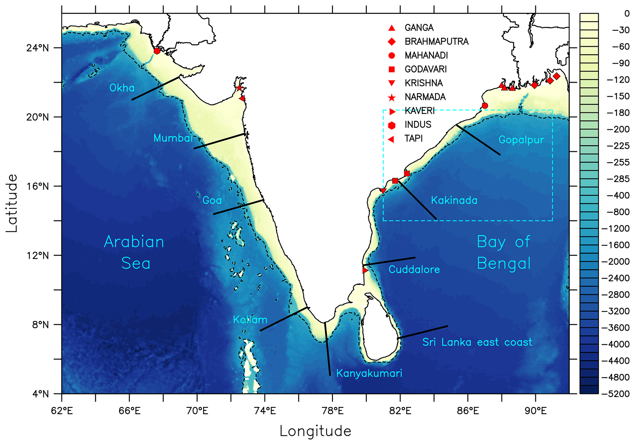
Figure 1 Study area depicting the bathymetry of the MITgcm domain in colour scale. The dashed black line represents the 1000 m bathymetry contour. The red symbols represent the discharge points of major river systems in India. The dashed blue box represents the region considered for eddy-induced transports. All transects are 3° in length (solid black lines).

2 Materials and methods

2.1 Model

2.1.1 MITgcm description and configuration

The MITgcm (Marshall et al., 1997) is configured for a regional domain (4–26° N, 62–92° E), which includes the AS and the BoB. This model solves Navier–Stokes equations by using Boussinesq approximation. Here we have chosen the hydrostatic approximation. The finite-volume approach is used over a staggered Arakawa-C grid. The third-order direct space–time advection scheme is used for temperature and salinity. This setup has a uniform high spatial resolution of $\mathrm{1}/\mathrm{20}$° (∼5 km), with 49 vertical levels in a z-coordinate system. Such a fine resolution allows the simulations to be eddy resolving. The vertical resolution is 5 m from the surface to 250 m depth and gradually decreases at a deeper depth. The maximum depth of the setup is 4500 m. Bathymetry is obtained from the General Bathymetric Chart of the Oceans (GEBCO) (Weatherall et al., 2020), having a high spatial resolution of 15 arcsec. We use K-profile parameterization (KPP) (Large et al., 1994) as the vertical mixing parameterization scheme and an MDJWF equation of state (McDougall et al., 2003). There are three lateral open boundaries along the western, eastern, and southern edges of the model domain. No-slip and free-slip boundary conditions are applied at the bottom and lateral boundaries respectively for velocities. An implicit free surface and a non-rigid lid condition are implemented for the surface pressure. The model is integrated over an optimized time step of 120 s and is designed using climatological forcing data. Initial temperature and salinity are prescribed from the World Ocean Atlas 2018 (WOA18) climatology (Locarnini et al., 2018; Zweng et al., 2019). To reduce the spin-up time and computational expenditure, the model is initialized with a warm start. For this, climatological zonal and meridional currents are prescribed from the Simple Ocean Data Assimilation (SODA) 3.12.2 dataset (Carton et al., 2018). Lateral boundary conditions, that is, temperature, salinity, and currents, are also prescribed from SODA 3.12.2 on a pentad climatological timescale. The model is forced with a daily climatology of 2 m air temperature, 2 m specific humidity, 10 m zonal and meridional wind, and net shortwave and longwave radiation as the atmospheric forcing, from the fifth-generation reanalysis (ERA5) (Hersbach et al., 2020). Precipitation is obtained from the Global Precipitation Measurement (GPM) level 3 (Huffman et al., 2015). Along with this, climatological river discharge from Dai and Trenberth (2002) is fed to the model using a point-source method to incorporate the effect of river runoff at the locations marked in red in Fig. 1. The model uses bulk formulae to calculate net heat and freshwater flux using the above parameters. The model is relaxed at the surface with monthly climatology of Multi-scale Ultra-high Resolution (MUR) v4.1 sea surface temperature (SST) (Chin et al., 2017) and Soil Moisture Active Passive (SMAP) sea surface salinity (SSS) (Tang et al., 2017) satellite data, prescribed every 10th day. The data links of all datasets are provided in the code and data availability section.

2.1.2 HYCOM model description

We used data of the assimilated HYbrid Coordinate Ocean Model (HYCOM) (Bleck, 2002) to perform a model-to-model comparison with the MITgcm simulations. The model is simulated at the Indian National Centre for Ocean Information Services (INCOIS; hereafter referred to as INC-HYC) and is an eddy-resolving model with a high spatial resolution of $\mathrm{1}/\mathrm{16}$° (∼6.25 km) over the IO (43.5° S–30° N, 20–120° E). It is one-way nested within a global HYCOM setup of $\mathrm{1}/\mathrm{4}$° (∼25 km) spatial resolution. The model equations are solved on the Arakawa-C grid using the finite-volume method. The second-order enstrophy conserving scheme is used to compute momentum advection (Bleck and Boudra, 1986; Bleck and Smith, 1990). Continuity equations and physical tracers such as temperature and salinity are computed using a second-order flux-corrected transport scheme (Iskandarani et al., 2005; Zalesak, 1979). The model has 29 vertical hybrid layers. This setup incorporates the Tendral Statistical Interpolation (T-SIS) data assimilation scheme, based on multivariate linear statistical estimation. A combination of GEBCO and the Earth TOPOgraphy 1 Arc-Minute (ETOPO1) global relief model is used as the model bathymetry. The atmospheric forcings, that is, 2 m air temperature, 2 m vapour mixture, surface downward and upward long- and shortwave radiation, precipitation, and 10 m zonal and meridional wind, are obtained from the NOAA Global Forecasting System (GFS). Wind stress is computed according to Kara et al. (2005), whereas bulk formulae used to calculate surface fluxes are referred from Kara et al. (2000). KPP (Large et al., 1994) is chosen as the vertical mixing scheme. Monthly climatological river discharge is used from the Naval Research Lab (NRL). The model is simulated for a 5-year hindcast period (2012–2016), and the state variables are written at daily intervals. We have computed daily climatology from these data. The technical report (https://incois.gov.in/documents/TechnicalReports/ESSO-INCOIS-CSG-TR-01-2018.pdf, last access: 25 October 2023) can be referred to for more details and exhaustive validation. The HYCOM-simulated data are reliable and perform reasonably well when compared with other data assimilation products such as NRL-HYCOM and the INCOIS-Global Ocean Data Assimilation System (GODAS).

2.2 Data

To validate the seasonal model SST and SSS, we used the Group for High Resolution Sea Surface Temperature (GHRSST) (Donlon et al., 2012) and Soil Moisture and Ocean Salinity (SMOS) SSS v8.0 level 3 (Boutin et al., 2023) datasets respectively. The GHRSST level 4 data by NASA's JPL is produced using the optimal interpolation method at 0.054° spatial resolution. The latest version of SMOS uses an improved de-biasing technique and is available at 0.259°×0.196° spatial resolution. Apart from these satellite datasets, we have also validated the model temperature and salinity with the gridded Coriolis Ocean Dataset for Reanalysis (CORA) v5.2 (Szekely et al., 2019) and RAMA buoy (McPhaden et al., 2009) (refer to Texts S3 and S4 in the Supplement). CORA v5.2 data have been produced using multiple in situ sampling techniques, such as Argo floats, drifters, gliders, moorings, etc. It has a spatial resolution of 0.5°, with data available from the surface to 2000 m depth. GlobCurrent zonal and meridional surface currents (Rio et al., 2014) were used to validate model-computed surface currents. These observational data, derived from satellite mean dynamic topography, are available at the surface and 15 m, as a sum of geostrophic and Ekman currents. These data have a spatial resolution of 0.25°. We computed monthly climatology for all these datasets and compared them with seasonal patterns of simulations.

2.3 Methods

We initialized the model with the December monthly climatology of ocean temperature and salinity from WOA18 and zonal and meridional currents from SODA 3.12.2. Boundary conditions were forced from SODA 3.12.2 for the climatological year on a pentad timescale. For appropriate selection of boundary conditions, we conducted a few sensitivity experiments using different reanalysis products (SODA 3.12.2, ECCOv4, and INCOIS-GODAS) and observed that SODA 3.12.2 was able to represent the ocean temperature, salinity, and circulation better in the domain than others. Similarly, ERA5 wind data were compared with wind from the RAMA buoy at various locations over the AS and BoB, and it was observed that ERA5 shows a strong correlation, lower RMSE, and low standard deviation compared with RAMA. Hence, we selected this dataset for the surface forcings. All forcing datasets were regridded to the model domain resolution. The model was spun up for 5 years. Based on the temporal evolution of kinetic energy, we found that it achieves a steady state after 5 years. The 6th-year model output was considered for our analysis. Model outputs were written on a pentad scale. To compute the transports, the transects were drawn by the following method. We drew a tangent vector at the curvature of each coastal point. Then, the normal vector of length 3° each was drawn beginning from the coast. Further, to calculate the alongshore and cross-shore current component, the angle of rotation was considered from the normal vector to the true north, in anticlockwise direction. The alongshore and cross-shore current components can be denoted as

$$\begin{array}{}\text{(1)}& {\displaystyle }\text{acomp}=\left(u\sin \right(\mathit{\theta })-v\cos (\mathit{\theta }\left)\right),\text{(2)}& {\displaystyle }\text{ccomp}=-\left(u\cos \right(\mathit{\theta })+v\sin (\mathit{\theta }\left)\right),\end{array}$$

where u and v are the zonal and meridional current components, and θ is the angle of rotation in radians. Here, acomp and ccomp are the alongshore and cross-shore current components respectively. The alongshore volume transport (AVT) and cross-shore volume transport (CVT) are computed in Sv ($\mathrm{1}\mathrm{Sv}=\mathrm{1}\times {\mathrm{10}}^{\mathrm{6}}$ m³ s⁻¹) following Stammer et al. (2003). The transports are computed by integrating in depth and along the length of the normal vector.

$$\begin{array}{}\text{(3)}& {\displaystyle }\text{AVT}=\iint \text{acomp}\mathrm{d}z\mathrm{d}n\text{(4)}& {\displaystyle }\text{CVT}=\iint \text{ccomp}\mathrm{d}z\mathrm{d}n\end{array}$$

Alongshore freshwater transport (AFT, in Sv) is computed referring to Rainville et al. (2022):

$$\begin{array}{}\text{(5)}& \text{AFT}=\iint \text{acomp}{\displaystyle \frac{(S_{\text{ref}}-S)}{S_{\text{ref}}}}\mathrm{d}z\mathrm{d}n,\end{array}$$

where S is the ocean salinity (psu), and S_ref is the reference mean salinity of 34.67 psu of the study area. It should be noted here that the freshwater fraction is always negative when S_ref<S as in the AS, irrespective of the orientation of the alongshore component. Thus, the sign convention of AFT in the AS will always be the inverse of the volume transport. However, in the BoB, the freshwater fraction will be mostly positive (S_ref>S). This causes the direction of AFT to be dependent only on the alongshore flow.

Alongshore heat transport (AHT) is computed in PW ($\mathrm{1}\mathrm{PW}=\mathrm{1}\times {\mathrm{10}}^{\mathrm{15}}$ W) referring to Stammer et al. (2003) and Chirokova and Webster (2006):

$$\begin{array}{}\text{(6)}& \text{AHT}=\mathit{\rho }{C}_p\iint \text{acomp}T\mathrm{d}z\mathrm{d}n,\end{array}$$

where T is ocean temperature (°C), ρ is seawater density (kg m⁻³), and C_p is the specific heat capacity of seawater (3898 $\mathrm{J}{\mathrm{kg}}^{-\mathrm{1}}\mathrm{°}{\mathrm{C}}^{-\mathrm{1}}$).

Components of eddy heat transport (EHT) are computed as

$$\begin{array}{}\text{(7)}& {\displaystyle }\text{ZEHT}=\mathit{\rho }{C}_p\iint uT\mathrm{d}z\mathrm{d}x,\text{(8)}& {\displaystyle }\text{MEHT}=\mathit{\rho }{C}_p\iint vT\mathrm{d}z\mathrm{d}y,\end{array}$$

where ZEHT is the zonal EHT, and MEHT is the meridional EHT. Similarly, the components of eddy freshwater transport (EFT) are computed as

$$\begin{array}{}\text{(9)}& {\displaystyle }\text{ZEFT}=\iint u{\displaystyle \frac{(S_{\text{ref}}-S)}{S_{\text{ref}}}}\mathrm{d}z\mathrm{d}x,\text{(10)}& {\displaystyle }\text{MEFT}=\iint v{\displaystyle \frac{(S_{\text{ref}}-S)}{S_{\text{ref}}}}\mathrm{d}z\mathrm{d}y.\end{array}$$

The net volume transport (NVT), net freshwater transport (NFT), net eddy heat transport (NEHT), net eddy freshwater transport (NEFT), and net heat transport (NHT) were obtained by summing their respective zonal and meridional components (Arora, 2021). The zonal and meridional components were computed at each grid point integrated over the upper 100 m.

3 Model validation

Model validation is a crucial step which ensures that the model accurately represents the complexities of oceanic dynamics. For validation, we compared the model SST (Fig. 2), SSS (Fig. 3), and surface currents (Fig. 4) with observations and computed biases. There are four seasons, which are distinguished as pre-summer monsoon (MAM), summer monsoon (JJAS), post-summer monsoon (ON), and winter (DJF). The characteristics of SST distribution across the AS and BoB are included in the Supplement (Text S1). The model setup simulates these seasonal SST patterns and compares well with both GHRSST and gridded Argo with an acceptable bias range. The model has a warmer bias in the northeastern AS during JJAS when compared with GHRSST (Fig. 2f) owing to an increase in net heat flux. In ON, the model SST is warmer along the western coast of India compared to the observations (Fig. 2g and k). Overall, we note that the model has a slightly warmer bias over parts of the northern AS and along the western coast where the shelf is wide with shallower water depth in the coastal regions. The heat gets trapped into the upper few metres, thereby increasing the surface net heat flux. We evaluated the model SST with observations statistically using a robust parameter, Pearson's correlation coefficient. We observe that simulated SST shows a strong positive correlation up to 0.98 with GHRSST and gridded Argo SST throughout the climatological year.

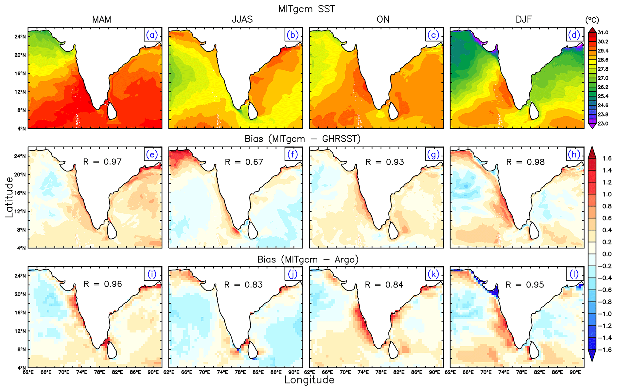
Figure 2 Seasonal climatology of SST (in °C) from (a–d) the MITgcm and its bias with (e–h) GHRSST and (i–l) Argo. R values represent Pearson's correlation coefficients.

Figure 3 Seasonal climatology of SSS (in psu) from (a–d) the MITgcm and its bias with (e–h) SMOS and (i–l) Argo. R values represent Pearson's correlation coefficients.

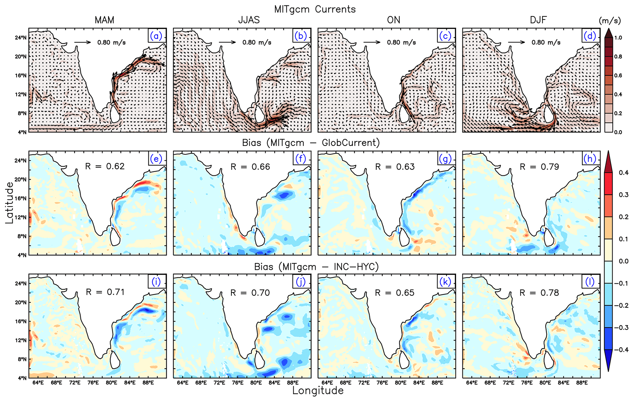
Figure 4 Seasonal climatology of surface currents overlaid with vectors (in m s⁻¹) from (a–d) the MITgcm and its bias with (e–h) GlobCurrent and (i–l) INCOIS-HYCOM. R values represent Pearson's correlation coefficients.

SSS is another important parameter governing the transports. The characteristics of SSS distribution across the AS and BoB are included in the Supplement (Text S2). The model captures the SSS spatial variations and seasonality well and conforms with the observed SSS. The salinity difference between the AS and BoB is substantial in all seasons, which is also simulated well by the model. In DJF, the model SSS is saltier in the eastern BoB, as compared to observations (Fig. 3h and l). This bias can be attributed to the slight overestimation in the eastern boundary forcing data, which influences the simulated SSS of this region. Statistically, the model SSS shows a high spatial Pearson's correlation with both SMOS and gridded Argo SSS in all seasons. We have also statistically validated the simulated subsurface temperature and salinity with RAMA buoys and gridded Argo data to a depth of 500 and 100 m respectively at various locations. This validation is included in the Supplement (Texts S3 and S4).

We validated the model currents with GlobCurrent observations and compared them with INC-HYC-simulated currents, averaged over the upper 15 m. The model-simulated currents show consistent agreement with both GlobCurrent and INC-HYC. The model also captures the transition in coastal currents like the WBC and EICC well. During JJAS, equatorward-flowing WICC brings waters from the AS near the southern Sri Lankan coast, where the Sri Lankan Dome presides. During the same period, the EICC forms over the northern BoB, which the model simulates well. By ON, the EICC dominates the eastern coast of India and brings relatively fresher water into the southeastern AS, causing temperature inversions and barrier layer formation along this region (Mathew et al., 2018). During DJF, the model simulates the anticyclonic circulation of the Laccadive High (LH) in the same region. In the AS, the WICC reverses its direction and flows poleward. We computed the bias of the current magnitude of our MITgcm with GlobCurrent and INC-HYC. The bias is well within limits, and model surface currents spatially correlate well with both datasets (Fig. 4e–l).

4 Results

4.1 Alongshore volume transport (AVT) and alongshore freshwater transport (AFT)

To analyse the volume transports, we selected nine transects and computed the AVT. The 3° width of the transects was selected to incorporate the coastal currents, which typically flow conforming to the 1000 m isobath (Amol et al., 2014; Mukherjee et al., 2014; Shetye et al., 1991a) (refer to Fig. 1). We considered three transects, each along the eastern (Gopalpur, Kakinada, and Cuddalore) and western (Okha, Mumbai, and Goa) coasts. Two transects are located along the southern coast of India (Kollam and Kanyakumari), and one transect is located along the eastern coast of Sri Lanka. The AVTs were plotted as a function over time to observe their seasonal and intraseasonal variability. Positive values indicate poleward transport, whereas negative values indicate equatorward transport. The black lines indicate the transport integrated over the upper 200 m depth (M_0–200 and H_0–200), and the red colour (M_200–1200 and H_200–1200) indicates the transport integrated from 200 to 1200 m depth to understand the seasonal variability over the surface and subsurface ocean.

Along the eastern coast, the seasonal cycle dominates the transport of the EICC (Mukherjee et al., 2014; Mukhopadhyay et al., 2020). A poleward transport during MAM, owing to the WBC and an equatorward flow during the ON season, is observed due to the EICC. However, we observe intraseasonal variability at Cuddalore. The flow of the transport reduces from north to south. It is interesting to note that the AVT is the highest at Gopalpur and the lowest at Mumbai, both being at almost the same latitude. In the west coast locations along the WICC, we observe weaker seasonal variations. We observe a dip at all three locations, i.e. Okha, Mumbai, and Goa, during the summer monsoon, which is attributed to the equatorward-flowing WICC. In the southern part, the AVT at Kollam uniformly deviates around its mean signal throughout the year, which has also been noted by the current pattern in Chaudhuri et al. (2020). The transport at Kanyakumari is dominated by the eastward-flowing southwestern monsoon current during the summer monsoon and the westward-flowing northeastern monsoon current during the winter. The strong poleward flow during the JJAS season indicates the transport of waters from the AS into the southwestern BoB. Cuddalore, Kollam, Kanyakumari, and the eastern coast of Sri Lanka are closer to the equatorial Indian Ocean and thus experience a stronger impact of remote forcing compared to other locations in the northern AS and BoB. The subsurface AVT over the western coast is of the same magnitude as compared to the surface. However, it is stronger along the eastern coast.

We also compared the MITgcm-simulated transport values with the ones from INC-HYC and computed correlation coefficients (Fig. 5). Statistically, we observe a strong positive correlation between the transport from both models, with the only exception being Cuddalore and Kanyakumari. The surface and subsurface transports over Gopalpur and Kakinada have opposite flows during MAM seasons, indicating a strong countercurrent seen in both the MITgcm and the INC-HYC model. The strongest subsurface AVT is observed at Cuddalore and the eastern coast of Sri Lanka. Our estimates are also consistent with the findings from Shetye et al. (1991b, 1996). The heat component of transport, i.e. AHT, has also been computed to provide a complete picture. The seasonality of computed AHT is similar to that of AVT (refer to Fig. S3 in the Supplement).

Figure 5 AVT (in Sv) of the MITgcm (solid lines) and INC-HYC (dashed lines). R represents the Pearson's correlation coefficient between the MITgcm and INC-HYC.

Along the Indian coasts, the analysis of freshwater transports is crucial. This importance arises from the significant contributions of precipitation and discharge to glacial meltwater, both of which are integral components of coastal dynamics. For this, we computed AFT by taking the double integral of the freshwater fraction and alongshore velocity component in length and depth at the same locations as the AVT (Fig. 6). We computed the AFT in sverdrup (volume) instead of kilograms per second (mass) to maintain uniformity. We observe some interesting patterns in the AFT variability. First, the directions of seasonal variations in AVT and AFT contradict each other on the western coast. However, they are similar on the eastern coast. This can be attributed to the role of salinity in both basins. Second, we note that the magnitude of AFT is an order lower than that of AVT. During February–April, the WBC transports freshwater poleward along the eastern coast. As the salinity in the BoB is always less than the reference (S_ref) and the alongshore current component is positive, the directions of AVT and AFT are the same in this period. As the summer monsoon arrives, we see a reversal in the flow of freshwater driven by the EICC due to a negative alongshore current component. This equatorward flow is prominent during October–November at Gopalpur and Kakinada. The AFT at Cuddalore flows equatorward by December–January. The contradictory behaviour of subsurface AFT can be observed at Gopalpur due to the countercurrent. On the western coast, we observe a positive AFT at Okha, Mumbai, and Goa during the summer monsoon. This can be attributed to the high precipitation along these regions in addition to the river runoff, which is discharged into the coastal AS (Behara et al., 2019). Moreover, at Kanyakumari, we observe two peaks, one during the JJAS season and the other during December. The first peak is attributed to the high precipitation, whereas the second peak is due to freshwater flow from the BoB to AS. The surface AFT estimates from the MITgcm conform well at all locations except Kanyakumari, with the AFT computed from INC-HYC (Fig. 6), as seen by the positive correlation.

Figure 6 AFT (in Sv) of the MITgcm (solid lines) and INC-HYC (dashed lines). R represents the Pearson's correlation coefficient between the MITgcm and INC-HYC.

4.2 Spatial variability of net volume transport (NVT) and net freshwater transport (NFT)

To understand the seasonal spatial transport over the domain, we computed NVT and NFT at each grid point integrated over the upper 100 m (Fig. 7). When analysing transports at transects along the coasts, the alongshore and components become pertinent. However, for a grid-wise computation in the domain, the net component involving the zonal and meridional information is a more robust and meaningful metric. As observed in previous sections, the transport along the coastal BoB is stronger as compared to the AS. In MAM, the MITgcm simulates a strong poleward NVT due to the WBC extending from 10–20° N. Simultaneously, a weaker westward flow (2.5 to 5 Sv) streams along the southern coast of Sri Lanka. During JJAS, a pair of cyclonic eddies situated over the northwestern BoB is observed. During this period, we also observed the Sri Lankan Dome along the eastern coast of Sri Lanka. It forms during early June and strengthens into a cyclonic circulation (Cullen and Shroyer, 2019). The NVT in this region exceeds 10 Sv during JJAS and weakens by ON as it moves northward. In ON, the EICC in the BoB has a discontinuous flow (Durand et al., 2009) and shifts equatorward along the southwestern BoB. By DJF, it is observed that the equatorward flow of the EICC is further carried westward by the northeastern monsoon current into the southeastern AS but remains confined between 4–6° N. This is simulated well by both models and is also reported by Zhang and Du (2012).

Figure 7 Seasonal spatial variability of NVT and NFT of the MITgcm. Positive values (red) indicate northward/eastward flow, whereas negative values (blue) indicate southward/westward flow.

We quantified the NFT as a percentage of NVT over different seasons to understand how much freshwater is advected by the WBC and EICC along the eastern coast of India. During MAM, the NFT of the WBC is 2.10 % of the NVT from the MITgcm. Low-saline water of 0.1–0.3 Sv is advected poleward in this period. In the JJAS season, the equatorward EICC transports around 0.2–0.4 Sv of freshwater. It is bounded between the head and northwestern BoB and transports most freshwater (6.03 %). Moreover, the major Indian rivers have the largest riverine discharge during this season (Dai and Trenberth, 2002). By ON, the equatorward NFT along the eastern coast of India reaches the southwestern BoB, and transport exceeds 0.4 Sv at a few locations. By this period, the NFT reduces to 4.86 % of the NVT, as the freshwater mixes with the saltwater. By DJF, the freshwater is further transported westward into the southeastern AS. The flow seems to be the strongest along the southeastern coast of India and the southern coast of Sri Lanka (>0.3 Sv). As the water propagates from the BoB into the southeastern AS, its freshness decreases slowly due to continuous mixing with saltier waters, and the NFT further reduces to 2.83 % of the NVT. Our results along the coast of Sri Lanka agree with Rainville et al. (2022).

4.3 Contribution of heat and freshwater transport due to eddies

4.3.1 Eddy heat transport along the eastern coast of India

In addition to the alongshore volume and freshwater transports, our eddy-resolving MITgcm setup allows us to look into the heat and freshwater transport by eddies. The BoB experiences significant mesoscale and submesoscale eddies (Chen et al., 2012; Cheng et al., 2018). For our analysis, we selected the northwestern BoB region to study the transport by mesoscale activities, as shown in Fig. 8. Kurien et al. (2010) reported that the generation of these eddies is driven by baroclinic instability due to the poleward-flowing WBC. Two eddy regions were identified where the eddies exist from April to July, and they extend up to 100 m depth in the vertical, which can be seen from the current vectors (Fig. 8a–c). Box 1 identifies an anticyclonic eddy (ACE) followed by a cyclonic eddy (CE). Box 2 identifies a CE which is the strongest in May and starts weakening in July. In Box 1, the ACE begins to dissipate by May, and the CE strengthens. This can be seen by the slight shoaling of mixed layer depth (MLD) and the shift in vertical velocity from downward (negative) to upward (positive) due to divergence at the eddy centre (Fig. 8e). The eddy-induced transports have been computed over the upper 100 m. The ZEHT shows a consistent eastward transport between 0.22–0.11 GW from April to July. The MEHT transitions from being northward at ∼0.07 GW by April–May to southward by June–July, reaching a maximum of −0.06 GW during June. The NEHT propagates in the eastern-northeastern direction, transporting 0.28–0.06 GW during the period.

Figure 8 (a–c) Sea level anomaly overlaid with current vectors depicting the cyclonic and anticyclonic eddies simulated along the eastern coast of India. Vertical profiles of ocean temperature, vertical velocity, and MLD for Box 1 (d, e) and Box 2 (g, h) and their computed zonal, meridional, and net eddy heat transports (f, i).

In Box 2, we observe strong upward vertical velocity during May–June. The MLD shoals from 30 to 20 m within June (Fig. 8h). The ZEHT transports a maximum of ∼0.52 GW in April and weakens to around 0.06 GW by July. Similarly, the MEHT has a southward transport of −0.18 GW in April, which transitions into weak northward transport of 0.06 GW by July. Overall, the NEHT shows that the eddy propagates in the east–west direction, transporting about 0.36–0.06 GW during the period.

4.3.2 Eddy freshwater transport along the eastern coast of India

The EICC in the BoB has been described as a discontinuous flow (Durand et al., 2009) due to possible eddy activity as a means of baroclinic or barotropic instabilities. We identified a CE transporting fresher water along the eastern coast with intensity peaking by the month of October. The eddy extends up to 100 m depth. The upwelling at the centre of the CE is evident due to the shoaling of the MLD (Fig. 9b). The eddy-induced ZEFT transports westward, intensifying around 0.08 Sv by the end of November, whereas the MEFT has a peak southward transport of 0.15 Sv by the end of October. The order of the computed MEFT matches with that of Lin et al. (2019). Overall, the NEFT shows that the eddy propagates in the southwestern direction, transporting up to 0.16 Sv freshwater during October–November.

Figure 9 (a) SSS overlaid with current vectors depicting the cyclonic eddy simulated along the eastern coast of India. Vertical profiles of ocean salinity, vertical velocity, and MLD for Box 1 (b, c) and their computed zonal, meridional, and net eddy freshwater transports (d).

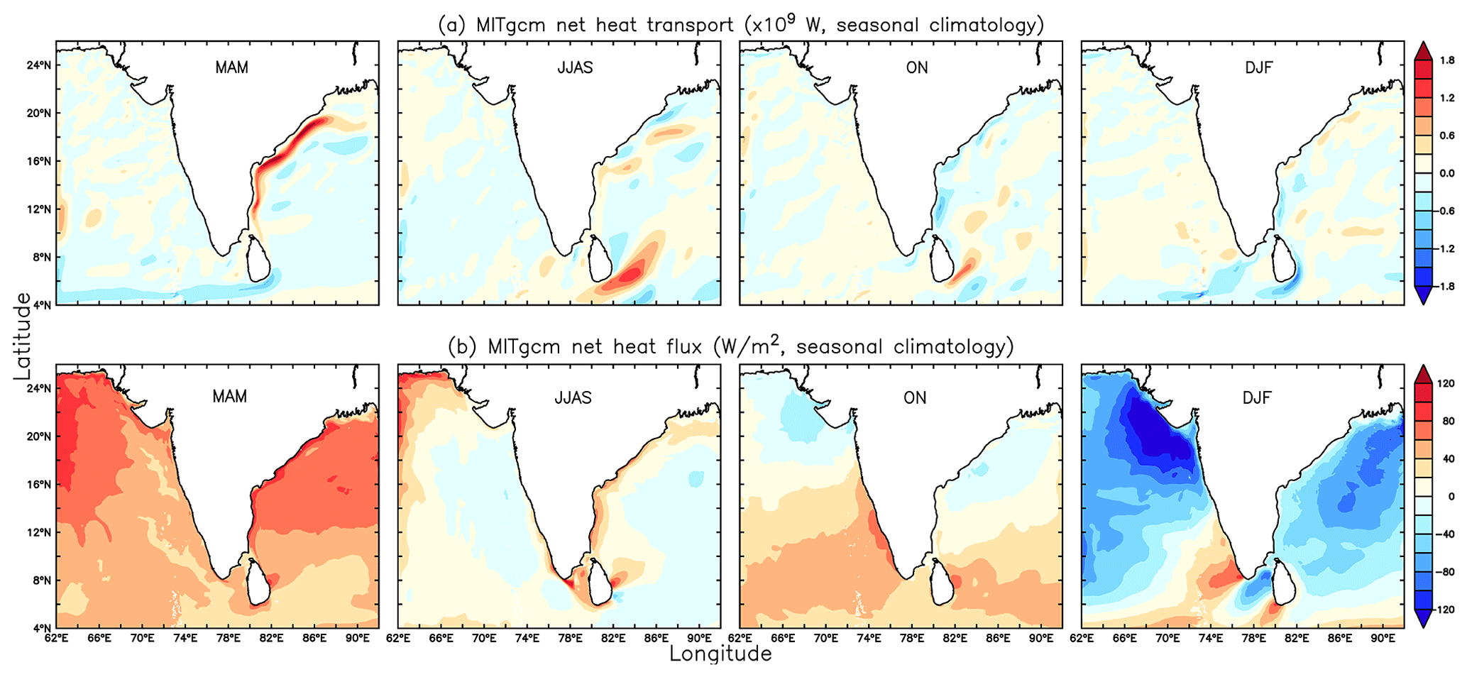
Figure 10 MITgcm-computed (a) seasonal NHT (GW, $\mathrm{1}\mathrm{GW}=\mathrm{1}\times {\mathrm{10}}^{\mathrm{9}}$ W) integrated over the upper 100 m. For panel (a), red indicates northward/eastward flow, whereas blue indicates southward/westward flow. (b) MITgcm-computed seasonal surface net heat flux (W m⁻²). For panel (b), red represents heat gain, and blue represents heat loss.

4.4 Net heat transport (NHT) and net heat flux

Studying the NHT in addition to volume transport provides a more comprehensive view, as heat transport is an important link influencing the dynamics of water movement. We aimed to understand the thermal component of the transports and its spatio-temporal variability in the NIO. In MAM, the WBC carries the warmer water along a strong poleward transport (Fig. 10a). With the onset of June, the NHT is prominently high along the Sri Lankan Dome. This cyclonic eddy is strengthened by JJAS, and the warm water is transported northward by ON. This is clear in the NHT signature of JJAS and ON. In the winter season, the heat transport is relatively low because of several factors.

The characteristics of net heat flux are considerably different from those of the NHT. The heat flux is primarily governed by atmospheric forcings and vertical mixing. During MAM, there is an increase in net shortwave radiation (Fig. 10b), and the winds are weak, which stalls the vertical mixing. This causes shoaling of the mixed-layer depth, increases stratification, and traps heat in the upper surface layers in almost the entire domain. In JJAS, we observe the cooling of surface waters due to rain-bearing clouds, which block incoming shortwave radiation (Das et al., 2016). This further prevents evaporation, leading to a net heat gain in JJAS. At the same time, the waters along the eastern coast of India in the BoB gain heat owing to stratification. By ON, net shortwave radiation decreases, and the wind direction reverses. The northeasterly cold dry winds cool the surface waters of the northern AS and BoB, which triggers convective mixing. We observe similar cooling near the southern tip of the mainland owing to latent heat release due to strong winds (Luis and Kawamura, 2000). The southeastern AS region has high heat flux throughout the ON, DJF, and MAM seasons.

4.5 Evaluation of meridional heat transport

To understand the meridional heat distribution and ventilation in the NIO basin by currents, we computed the MHT in the AS and BoB basins for the MITgcm. We zonally integrated the MHT at each latitude, over the upper 100 m. The MHT is plotted as a function over time (Fig. 11). The MHT pattern of the AS is considerably different from that of the BoB. The AS MHT has a prominent seasonal signature with a southward transport exceeding 1.25 PW during JJAS and a northward transport (>1 PW) during DJF (Fig. 11a). In other words, the heat flows out from the AS into the equatorial Indian Ocean during the summer monsoon, and the heat flows into the AS in the winter (Garternicht and Schott, 1997). The latitudinal band between 6–12° N sees the strongest positive and negative signals of MHT. The reversal in the direction of the MHT occurs during the MAM and ON seasons. The BoB MHT is observed to be weaker than the AS MHT (Fig. 11b). Overall, the MHT does not exceed ±0.75 PW in the BoB basin. We observe a weak southward MHT (∼0.25 PW) during the JJAS season and a weak northward MHT (∼0.5 PW) during the DJF and MAM seasons. The values agree with Shi et al. (2002). Along 6° N latitude, ∼0.5 PW of southward MHT exists between February and April. The lower-latitudinal band between 4–6° N shows a comparatively stronger intraseasonal modulation of MHT. We find small bursts of northward MHT between November–January and April–May and southward MHT during JJAS. This is influenced by the transport from the equatorial IO.

Figure 11 Meridional heat transport (MHT, in PW) computed over the upper 100 m using the MITgcm for the AS and BoB. The red colour indicates northward transport, and the blue colour indicates southward transport.

5 Discussion

This study indicates that the transports on the eastern and western coasts of India are different from each other, with the transport along the eastern coast being largely seasonal, while on the western coast, the transports are mostly modulated by intraseasonal oscillations. This is mostly because the transport on the eastern coast is governed by the EICC, which is more seasonal, while on the western coast, more intraseasonal WICC dominates. The modelled AVT estimates are consistent with earlier findings on both coasts, as well as along the Sri Lankan coast (Anutaliya et al., 2017; Chaudhuri et al., 2020). In the case of AFT, we observed evidence of countercurrents causing the directions of surface and subsurface transport to counter each other. Higher river runoff during the monsoon season governs the peak in the AFT at both coasts, whereas at Kanyakumari we observed high transport in December due to freshwater flow from the BoB to the AS. Along the eastern coast of Sri Lanka, the freshwater transport peaks during November, a month before that of Kanyakumari. This analysis shows interesting contrasts in the AVT on the eastern and western coasts. In the western coasts, seasonal variations in AFT and AVT oppose each other due to salinity dynamics. In contrast, the eastern coast shows similar seasonal trends in AVT and AFT, reflecting the influence of freshwater inputs from precipitation and river discharge.

The model setup also simulates climatological eddies and the Sri Lankan Dome. The climatological eddies along the eastern coasts are active during June–July, but by August–September, they get disrupted due to an equatorward transport initiated by the EICC. The seasonal spatial NFT pattern is similar to that of spatial NVT. However, its value is an order less than NVT. Important seasonal dynamics that we understand from our analysis is that, during the pre-monsoon period, the poleward transport by the WBC is relatively low. However, in the monsoon season, the EICC significantly enhances equatorward freshwater transport due to high riverine discharge. As the season progresses into ON, the freshwater transport decreases as it mixes with saltwater. By winter, the transport continues westward into the Arabian Sea, with the intensity of flow decreasing as it further mixes with saltier waters.

Eddies are generated in the northwestern BoB due to baroclinic instability driven by the poleward-flowing WBC. The identified eddy regions in this study exhibit distinct seasonal patterns, with the presence of anticyclonic and cyclonic eddies impacting the vertical structure and transport dynamics. One of the interesting findings was that the eddies with persistent cyclonic circulation influence the MLD and vertical velocity patterns significantly more than the eddies where the transition from anticyclonic to cyclonic circulation takes place. In August–November, however, the eddies formed in the BoB transport freshwater zonally and meridionally, with their intensity peaking by the end of September. These mesoscale eddies play an important role in transporting the freshwater accumulated in the head of the BoB region along the coast. The westward and southward transports of freshwater by the eddies show the interaction between mesoscale eddies and coastal currents. The consistency of the transports computed matches with previous studies and further validates the model simulations.

The NHT analysis shows the significant role of heat transport in influencing water movement dynamics in the northern Indian Ocean (NIO). In the pre-monsoon season, the WBC's poleward transport of warmer water establishes a strong thermal gradient. The winter season shows a decline in heat transport due to seasonal atmospheric conditions, which highlights the influence of cooler, drier winds and reduced solar radiation. Net heat flux patterns are primarily driven by atmospheric conditions and vertical mixing processes. In MAM, the increased shortwave radiation and weak winds result in stratification and heat entrapment in the upper ocean layers. In JJAS, monsoon clouds reduce incoming radiation, thereby cooling the surface waters. Besides this, large evaporation results in the release of latent heat, which increases cooling largely in the open waters (Das et al., 2016). The western AS is saturated due to an increase in the specific humidity of air (Pinker et al., 2020). Post-monsoon, the reduction in net heat flux is attributed to heat loss in the form of latent heat, which is further intensified by DJF in these parts of the basin (Kumar and Prasad, 1999). The southeastern AS maintains high heat flux due to the export of freshwater from the southwestern BoB and a downwelling Rossby wave that creates a thick barrier layer and prohibits vertical mixing, thus capping heat in the upper layers (Mathew et al., 2018).

The MHT in the AS shows a clear seasonal reversal, driven by the reversal of winds along with meridional Ekman transports and vertical thermal wind shear (Lee and Marotzke, 1998; Schott and McCreary, 2001; Wacongne and Pacanowski, 1996). This seasonal pattern is influenced by the annual bi-mode westward-propagating Rossby wave, particularly in the latitudinal band between 6–12° N (Brandt et al., 2002). The reversal in MHT direction during the MAM and ON seasons aligns with known wind and circulation changes. The weakening of the summer monsoon impacts Ekman transport, leading to weaker southward MHT and further warming of the AS (Pratik et al., 2019; Swapna et al., 2017). In contrast, the BoB exhibits weaker MHT due to higher stratification and weaker winds, which result in slower circulation and poor vertical mixing (Mahadevan, 2016; Mallick et al., 2020; Shenoi, 2002). Overall, we understand that NIO becomes a heat source (sink) during the summer (winter) season. The heat stored in the upper waters is flushed out due to an overall southward transport during March–September, whereas water from the equatorial Indian Ocean is brought in by the northward transport during November–February.

6 Summary

Our high-resolution MITgcm setup, as demonstrated in this study, provides a comprehensive understanding of volume, freshwater, and heat transport dynamics in the northern Indian Ocean. The eddy-resolving capability and finer bathymetry in high-resolution modelling improve the overall estimates of exchange along and in the coastal waters. Major patterns observed are that the alongshore volume transport (AVT) is stronger on the eastern coast and is highly seasonal, as compared to the western coast, where it is influenced by large intraseasonal oscillations. Seasonal variations between AVT and alongshore freshwater transport (AFT) along the western coast show a contradiction, while on the eastern coast, they display in-phase behaviour. This depends mostly on the intricate coastal dynamics influenced by salinity variations in the AS and BoB. The eddy-resolving setup allowed us to identify eddies and their interaction with coastal currents. These eddies help in exchanging heat and freshwater along the coastal waters. The relation between NHT and net heat flux illustrates the role of coastal currents and equatorial forcing in dissipating heat within the coastal waters. Another important finding is that the meridional heat transport (MHT) is stronger in the AS compared to the BoB. The MHT plays a crucial role in flushing heat out during summer monsoon seasons and bringing equatorial waters in during the winter season. The model setup successfully simulates these vital climatological patterns, emphasizing the significance of high-resolution modelling in understanding the complex ocean dynamics of this region.