Intense anticyclones at the global Argentine Basin array of the Ocean Observatory Initiative

We analyzed physical oceanic parameters gathered by a mooring array at mesoscale spatial sampling deployed in the Argentine Basin within the Ocean Observatory Initiative, a National Science Foundation major research facility. The array was maintained at 42^∘ S and 42^∘ W, a historically sparsely sampled region with small ocean variability, over 34 months from March 2015 to January 2018. The data documented four anticyclonic extreme-structure events in 2016. The four anticyclonic structures had different characteristics (size, vertical extension, origin, lifetime and Rossby number). They all featured near-inertial waves (NIWs) trapped at depth and low Richardson values well below the mixed layer. Low Richardson values suggest favorable conditions for mixing. The anticyclonic features likely act as mixing structures at the pycnocline, bringing heat and salt from the South Atlantic Central Water to the Antarctic Intermediate Waters. The intense structures were unique in the 29-year-long satellite altimetry record at the mooring site. The Argentine Basin is populated with many anticyclones, and mixing associated with trapped NIWs probably plays an important role in setting up the upper-water-mass characteristics in the basin.

1 Introduction

The Argentine Basin is a very active region of the Southern Ocean with unique oceanographic characteristics and contrasted water masses (Fig. 1a) (Reid et al., 1997). The Malvinas Current (MC), the major western boundary current of the Argentine Basin, flows northward following the Subantarctic Front (SAF) and, at about 38^∘, encounters the warm and salty Brazil Current. The Brazil Current is the western boundary current of the South Atlantic Subtropical Gyre bounded by the Subtropical Front (STF) (Peterson and Stramma, 1991; Gordon and Greengrove, 1986) (Fig. 1a). The Brazil–Malvinas Confluence is a complex highly dynamic region populated with meso- and submesoscale structures such as eddies, rings, filaments, intrusions and meanders (e.g., Orue-Echeverria et al., 2019; Artana et al., 2021). The eddy kinetic energy (EKE) features a C-shape pattern with values above $\mathrm{800}\times {\mathrm{10}}^{-\mathrm{4}}$ m² s⁻² that extends from the Brazil–Malvinas Confluence (EKE reaching $\mathrm{1000}\times {\mathrm{10}}^{-\mathrm{4}}$ m² s⁻²) to the southern Argentine Basin (Fig. 1b). A local minimum of EKE in the center of the basin (Fig. 1b) corresponds to the Zapiola anticyclonic circulation (ZAC, Fig. 1a) (Saraceno et al., 2009).

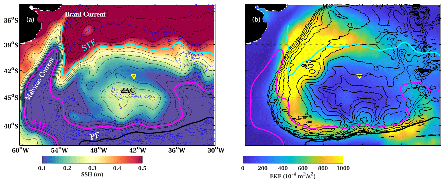
Figure 1 Mean sea surface height (SSH) (a) and mean eddy kinetic energy (b) over the period 1993–2020 from satellite altimetry. The cyan, magenta and black contours represent the mean position of the Subtropical Front (STF, SSH = 0.40 m), Subantarctic Front (SAF, SSH = 0 m) and Polar Front (PF, SSH = 0.34 m). The yellow triangle indicates the location of the OOI array. In (a), black isolines are every 5 cm, and blue isolines represent isobaths (6000, 5000, 3000 and 2000 from Sandwell and Smith (1994)). In (b), black isolines are potential vorticity contours plotted every $\mathrm{5}\times {\mathrm{10}}^{-\mathrm{9}}$ s⁻¹ m⁻¹. ZAC stands for Zapiola anticyclonic circulation, and PF stands for Polar Front.

Information on eddies in the Argentine Basin mostly comes from satellite altimetry (e.g., Fu et al., 2006; Saraceno and Provost, 2012; Mason et al., 2017) as in situ time series are scarce in this region. The only mooring data were obtained in the boundary currents, either in the Malvinas Current (e.g., Artana et al., 2018) or the Brazil Current (e.g., Meinen et al., 2017), or only at depth near the bottom (e.g., Weatherly, 1993). However, due to the spatial and temporal sampling of present satellite altimetry missions, only a portion of the mesoscale activity can be monitored as eddies with radius smaller than 40 km are attenuated in satellite altimetric maps (e.g., Chelton et al., 2011; Ballarotta et al., 2019).

Within the Ocean Observatory Initiative (OOI, http://www.oceanobservatories.org, last access: 20 June 2023), mooring arrays were deployed to provide sustained open-ocean observations in high-latitude areas that have been historically sparsely sampled due to severe weather conditions (e.g., Smith et al., 2018). These arrays collect multidisciplinary data to address science questions related to ocean–atmosphere exchanges, climate variability, ocean circulation, ecosystems, the global carbon cycle, turbulent mixing and biophysical interactions (e.g., Ogle et al., 2018; Palevsky et al., 2018; Josey et al., 2019). Among the OOI mooring arrays, the Argentine Basin global array was deployed and maintained at 42^∘ S and 42^∘ W over 34 months from March 2015 to January 2018 (Fig. 1a). The mooring array was located to the south of the mean position of the Subtropical Gyre and to the north of the Zapiola anticyclonic circulation (Fig. 1a) in a region with small westward mean surface geostrophic velocities (−0.02 m s⁻¹) and weak mean eddy kinetic energy ($\mathrm{145}\times {\mathrm{10}}^{-\mathrm{4}}$ m² s⁻²) (Fig. 1). We concentrated on the ocean physical conditions encountered during those 3 years in this remote and never-sampled environment. The array documented unexpected extreme mesoscale structures, which are the focus of this work. We aimed at providing elements of response to the following questions. What are these mesoscale structures? Where do they come from? How often do they occur? Do they impact mixing?

The paper is organized as follows. Section 2 presents an overview of the OOI ocean physical dataset. Section 3 focuses on three extreme events recorded by the array. They are identified in satellite altimetry as ocean anticyclonic structures with distinct characteristics and origins. Section 4 investigates high-frequency variations (< 1 d) during the events, in particular near-inertial motions and the possible occurrence of mixing. Section 5 summarizes and concludes the paper.

2 The global Argentine array: overview

2.1 Mooring setup

Moorings from the global Argentine array were deployed for the first time in March 2015 (https://oceanobservatories.org/array/global-argentine-array/, last access: 20 June 2023) below Jason ground track #76 and # 35 (Fig. 2a). The ocean depth at the mooring array was 5200 m. Moorings were recovered and redeployed at the same position in October 2015 and September 2016. January 2018 was the end of the operations in the Argentine Basin with the final mooring recovery. At each visit, CTD (conductivity, temperature and depth) casts with water sampling were performed at the mooring site for instrument calibration (https://oceanobservatories.org/array/global-argentine-array/, last access: 20 June 2023). The array comprised four moorings in a triangular configuration (Smith et al., 2018): the flanking moorings A and B were at the two northern corners of the triangle, and the paired surface and APEX (Autonomous Profiling Explorer) profiler moorings occupied the southern corner (Figs. 1 and 2).

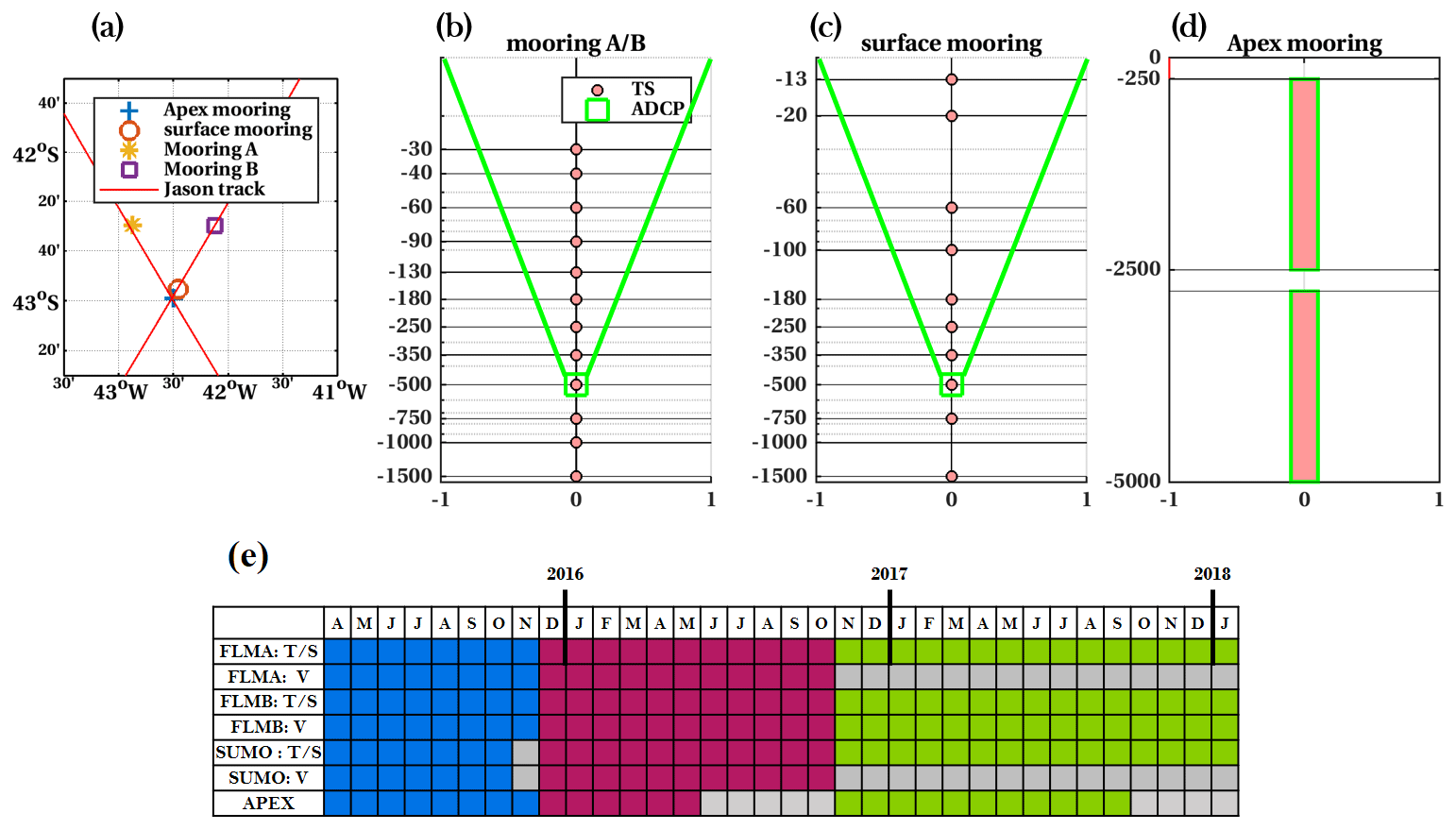
Figure 2 (a) Location of OOI moorings. Schematics of the northern moorings A and B (b), surface mooring (c) and APEX profiler mooring (d). The red circles mark the depth of temperature and salinity measurements, and the green squares mark the velocity measurements. Note that the vertical axis (depth in meters) in (b) and (c) is in log scale. (e) Record length for deployment 1 (blue), deployment 2 (red) and deployment 3 (green). Gray squares correspond to missing data.

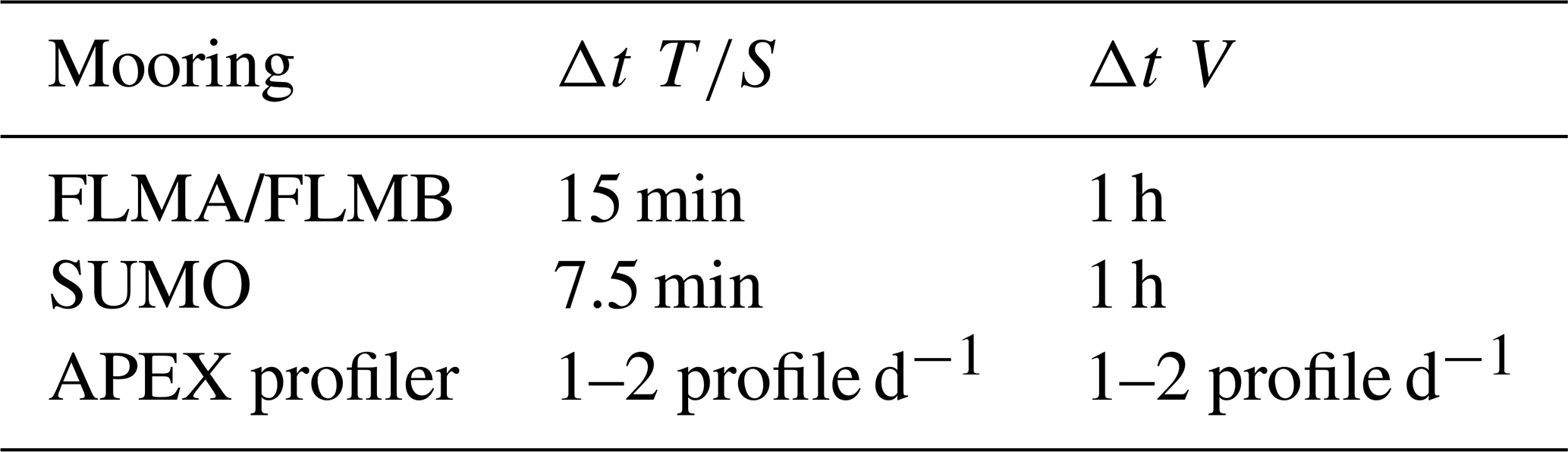
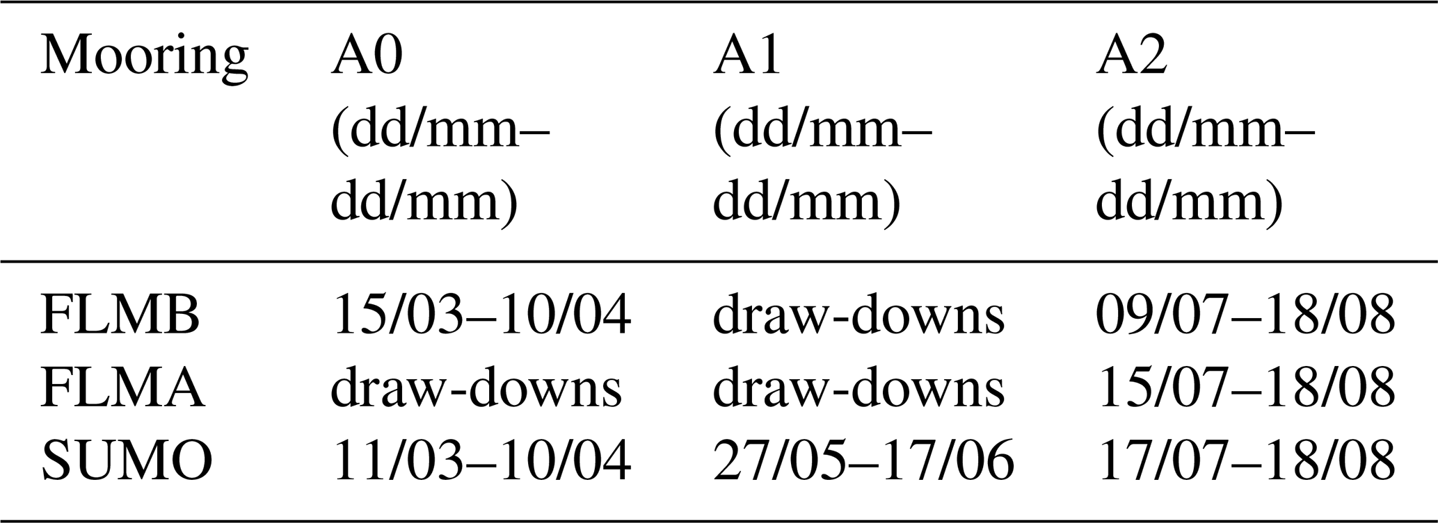
The two identical flanking moorings A and B (FLMA and FLMB, 62 km apart) comprised 12 microcats fixed at specific depths between 30 and 1500 m and an upward-looking RDI (RD instrument) 75 kHz long-range acoustic Doppler current profiler (ADCP) located at 500 m and measuring velocity profiles (Fig. 2b). The time sampling of the microcats and ADCPs was 15 min and 1 h, respectively (Table 1). The surface mooring (SUMO) had 10 microcats at fixed depths between 13 to 1500 m depth and an upward-looking ADCP RDI (75 kHz long range) at 500 m (Fig. 2c). The time sampling was 7.5 min for the microcats and 1 h for the ADCP (Table 1). The OOI ADCP data had a total of 52 bins of 10 m vertical resolution. The profiler mooring (APEX), 7 km away from SUMO, was a subsurface mooring equipped with two wire-following McLane moored profilers (Fig. 2d). The profilers performed one to two profiles per day, continuously sampling ocean variables (in particular temperature, salinity and zonal and meridional velocities) over specified depth intervals (250–2445 m for the upper profiler and 2470–4605 m for the lower one).

Table 1 Time sampling (Δt) of the mooring instruments.

The data processing of the physical variables is detailed in Artana et al. (2020). We removed spikes from temperature and salinity. The measurement quality of the mooring sensors, assessed by comparison with shipboard measurements (CTD profiles and bottle measurements) taken near the moorings during deployment and recovery cruises, was nominal (accuracy of 0.02 for salinity and 0.002 ^∘C for temperature). Hereafter practical salinity scale (EOS80) is used.

ADCP from mooring A (FLMA) and the surface mooring (SUMO) did not work during the third deployment (Fig. 2e). Gaps in the upper layer occurred when FLMB and FLMA underwent vertical excursions due to strong currents. Data return was almost 100 %, except for near-surface velocity measurements and periods of mooring draw-downs. Spiky and noisy patterns were often found in winter, concurrent with strong winds sometimes down to 150 m. They were identified and discarded.

2.2 Hydrography in the upper 1500 m (2015–2017)

The data return at the SUMO mooring is high in 2016, while data are more incomplete in 2015 and 2017 (Fig. 3). The temperature time series in the upper 100 m show a marked seasonal cycle, with a range of 10 ^∘C at the surface and 6 ^∘C at 100 m (pink and green curves in Fig. 3). Waters at 60 and 100 m depth are saltier than at shallower levels in summer by about 0.11 (Fig. 3b). In contrast, as winter mixed layers often exceed 100 m, temperatures and salinities are homogeneous in the first 100 m, and the pink (13 m), red (20 m) and dark-green (60 m) curves are hidden behind the light-green curve (100 m) in Fig. 3 from the end of May to the end of October.

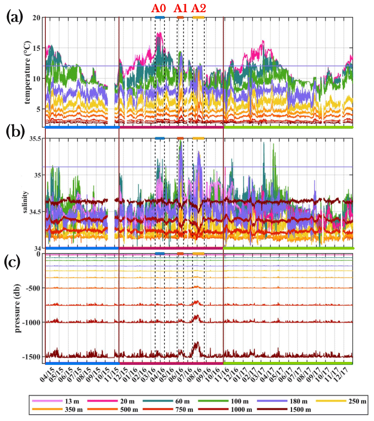
Figure 3 Temperature (a), salinity (b) and pressure (c) time series at the depths (indicated with colors) sampled at SUMO. The horizontal purple line in (a) (respectively (b)) corresponds to the mean plus 3 standard deviations of the temperature (respectively salinity) at 180 m. The color bars in the x axis delimit the three deployments: deployment 1 (blue), deployment 2 (red) and deployment 3 (green). Three events labeled A0, A1 and A2 stand out.

On top of the seasonal cycle, the time series show large variations of weekly to monthly duration that extend in the water column. Two temperature (T) and salinity (S) extrema, labeled A1 and A2, exceed 3 times the standard deviation (in T and S) at 180 m (purple curve in Fig. 3a and b). A1 and A2 happened in austral winter 2016 (Table 2). They were associated with warm and salty waters (T>10 ^∘C and S>35). During A2, the instruments below 500 m were lifted up by about 100 m at 1000 m depth and 200 m at 1500 m depth (brown curves in Fig. 3c). Another remarkable event, labeled A0, occurred around mid-March 2016 and featured the highest recorded surface temperature (T>17 ^∘C at 20 m) (pink curve in Fig. 3 and Table 2).

The θ–S diagram from SUMO data documents the water masses occupying the upper 1500 m of the water column (Fig. 4). Light densities with σ_θ less than 27.00 kg m⁻³ correspond to South Atlantic Central Water (SACW) for salinities larger than 34.2 and to Subantarctic Surface Water (SASW) for the lower salinities (Maamaatuaiahutapu et al., 1994). The salinity minima in the density range between 27.00 and 27.33 kg m⁻³ are associated with Antarctic Intermediate Waters located between 200 and 500 m (orange and yellow curves in Fig. 3b). Waters with densities larger than 27.33 kg m⁻³ in Fig. 4 correspond to Upper Circumpolar Deep Water (UCDW). The second-deployment data (red in Fig. 4) result in distinctive patterns in the θ–S diagram, where the extrema observed in Fig. 3 (A0, A1 and A2) stand out. The cloud spread in the θ–S diagram is considerably reduced when considering daily averaged data instead of full-resolution data (7.5 min), indicating large, high-frequency fluctuations in temperature and salinity (Fig. 4a and b).

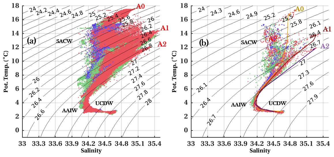
Figure 4 (a) θ–S diagram for each deployment from the surface mooring data (sampling every 7.5 min). First deployment in blue, second deployment in red, and third deployment in green. (b) Same as (a) with daily averaged data. Daily profiles for 1 April, 9 June and 7 August 2016 corresponding to A0, A1 and A2 are indicated in (b).

FLMA and FLMB did not move much during deployments 1 and 3, while they underwent large draw-downs during deployment 2 (Fig. A1 in the Appendix and Table 2). The A0 event led to vertical excursions of 100 m at 1500 m depth at FLMA, while FLMB remained still (Fig. A1 in the Apendix and Table 2).

Event A1 in May 2016 led to vertical excursions in excess of 400 m at FLMA and FLMB and to the collapse of the APEX mooring (Fig. A1 in the Appendix and Table 2). As a result, the APEX mooring did not sample A1 and A2 events.

Table 2 Dates of events at each mooring. No date is indicated during strong draw-downs.

2.3 Velocities

FLMB ADCP continuously functioned over the three deployments, while the ADCP from SUMO and FLMA did not work during the third deployment (Figs. 5, 2e). The largest velocities (peaking at 0.9 m s⁻¹) are observed in 2016 in the time series recorded by the three ADCPs (at SUMO, FLMA and FLMB) and are associated with A0, A1 and A2 (Fig. 5). To the first order, velocity components were rather homogeneous in the vertical (Fig. 5), and statistics for vertically averaged velocities are presented in Table A1 in Appendix A2.

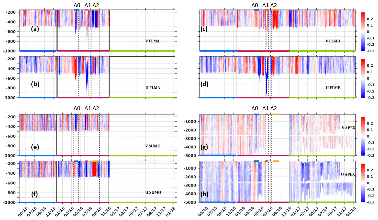
Figure 5 Meridional (V) and zonal (U) velocity time series (m s⁻¹) from FLMA ADCP (a, b), FLMB ADCP (c, d), SUMO ADCP (e, f) and APEX Aquadopp (g, h). The upper level is 150 m at all moorings. Time sampling for the ADCPs was 1 h, while the APEX profiler made a velocity profile per day. The APEX profiler did not sample the first 250 m.

Over the three deployments, the vertically averaged mean zonal velocity at FLMB is westward (−0.02 m s⁻¹), and the vertically averaged mean meridional velocity is northward (0.01 m s⁻¹). The meridional and zonal velocity components of the ADCPs recurrently changed sign, leading to small mean values (< 0.04 m s⁻¹) and larger standard deviations (> 0.08 m s⁻¹) (Table A1 in the Appendix and Fig. 5). The second deployment presents the largest standard deviations and EKE values. The standard deviations were reduced by about 1 to 2 cm s⁻¹ and EKE by 20 % when considering daily velocities (Table A1 in the Appendix).

Vertically averaged velocities between 300 and 480 m from the APEX profiler and the nearby SUMO are correlated (>0.7 above 99 % confidence level). APEX mooring velocities confirm that currents are rather barotropic in the region over the 5000 m depth (Fig. 5g–h).

The surface daily geostrophic velocities derived from satellite altimetry at $\mathrm{1}/\mathrm{4}{}^{\circ }$ (distributed by Copernicus Marine Service, CMEMS, http://marine.copernicus.eu/, last access: 20 June 2023) are in good agreement with the vertically averaged velocities at SUMO, FLMA and FLMB in terms of means, standard deviations and EKE (Table A1 in the Appendix). Satellite EKE was small during deployments 1 and 3 (< $\mathrm{100}\times {\mathrm{10}}^{-\mathrm{4}}$ m² s⁻²) and doubled during deployment 2 (> $\mathrm{200}\times {\mathrm{10}}^{-\mathrm{4}}$m² s⁻²), which is consistent with in situ velocities.

Figure 6 The 30 d low-pass-filtered altimetry-derived EKE at the mooring array location. The horizontal dashed black line indicates the mean, and the blue line marks the value of the mean plus 1.5 standard deviations. The vertical red lines show the period of the mooring deployment.

A 29-year-long surface EKE time series was derived from satellite altimetry at the array site (Fig. 6). The 29-year-long EKE time series does not feature any significant trend (Mann–Kendall test applied). Year 2016 stood out, with EKE values of $\mathrm{1000}\times {\mathrm{10}}^{-\mathrm{4}}$ m² s⁻² (Fig. 6).

3 The three events A0, A1 and A2

The three events featured daily average velocity amplitudes in excess of 0.3 m s⁻¹ at the three moorings (SUMO, FLMA and FLMB)(Fig. 7a, b, c). The velocity signal at A0 was smaller (> 0.3 m s⁻¹) than at A1 and A2 (> 0.5 m s⁻¹). APEX mooring documented the A0 event and showed that A0 velocity anomalies were bottom reaching (Fig. 5g and h). During the A0 event (April 2016), vertically averaged meridional velocities at FLMB were of opposite sign to those at FLMA and SUMO, while zonal velocities varied together (larger amplitude at FLMA) (Fig. 7d and e). During A1, velocities at the three moorings were in phase (Fig. 7d and e). Event A2 comprised two velocity maxima at the three moorings, A2^′ (peaking at 0.7 m s⁻¹ at FLMB) and A2^′′ (0.8 m s⁻¹ at SUMO) (Fig. 7a, b, c).

3.1 Identification of A0, A1 and A2 events in satellite altimetry

We compared altimetry-derived surface geostrophic velocities (SGV) time series at the 3 moorings to the vertically averaged in situ velocities time series during A0, A1 and A2. The vertical averages (full lines in Fig. 7d and e) cover the depth range 150–450 m for SUMO and variable depth ranges for FLMA and FLMB as the moorings underwent significant vertical excursions (Fig. 7a and b). The SGV times series (dashed lines in Fig. 7d and e) match vertically-averaged observations in terms of amplitude and direction (Fig. 7d and e). The agreement between SGV and in situ velocities is good during event A1 (root-mean-squared difference, RMSD, less than 0.08 m s⁻¹ for u and v at all moorings). During events A0 and A2, satellite-derived meridional velocities at FLMA and FLMB are smaller than vertically averaged in situ velocities by about 0.2 m s⁻¹ (50 % of the amplitude) and the RMSD (bias removed) are of the order of 0.1 and 0.09 m s⁻¹ respectively (Fig. 7d).

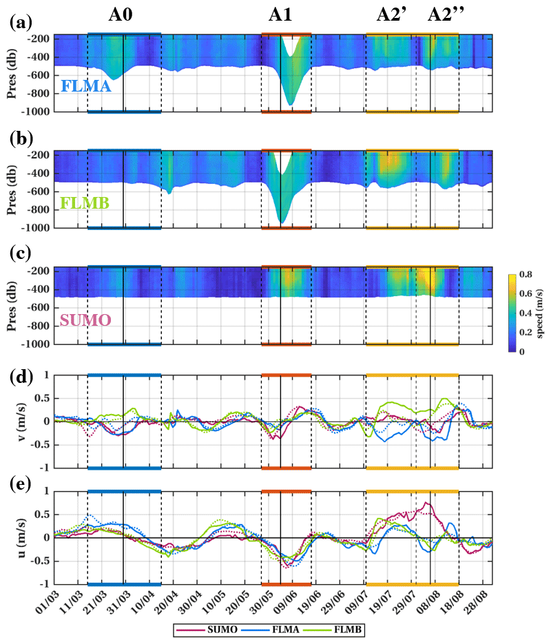
Figure 7 Daily averaged time series of velocity amplitude (m s⁻¹) from FLMA (a), FLMB (b) and SUMO (c). (d–e) Vertically averaged velocity time series from SUMO (red), FLMA (blue) and FLMB (green), where (d) is the meridional component and (e) is the zonal component. The dashed lines in (d)–(e) are surface geostrophic velocities derived from satellite altimetry co-localized at the mooring locations. The x axis is time (mm/yy). Vertical dashed lines bound A0, A1 and A2^′ and A2^′′. Black vertical lines correspond to dates considered in Fig. 8.

We identified the structures associated with A0, A1 and A2 in the satellite altimetry maps (Fig. 8). A video supplement shows the evolution of the SSH and velocity fields from January to September 2016 and provides information regarding the origin and fate of the structures.

A0 corresponds to the boundary of an elongated meander of the STF passing in the vicinity of the mooring array (Fig. 8a); A1 corresponds to a large anticyclonic eddy (Fig. 8b); and A2 corresponds to two small anticyclonic eddies, A2^′ and A2^′′ (video supplement; Fig. 8c shows A2^′′).

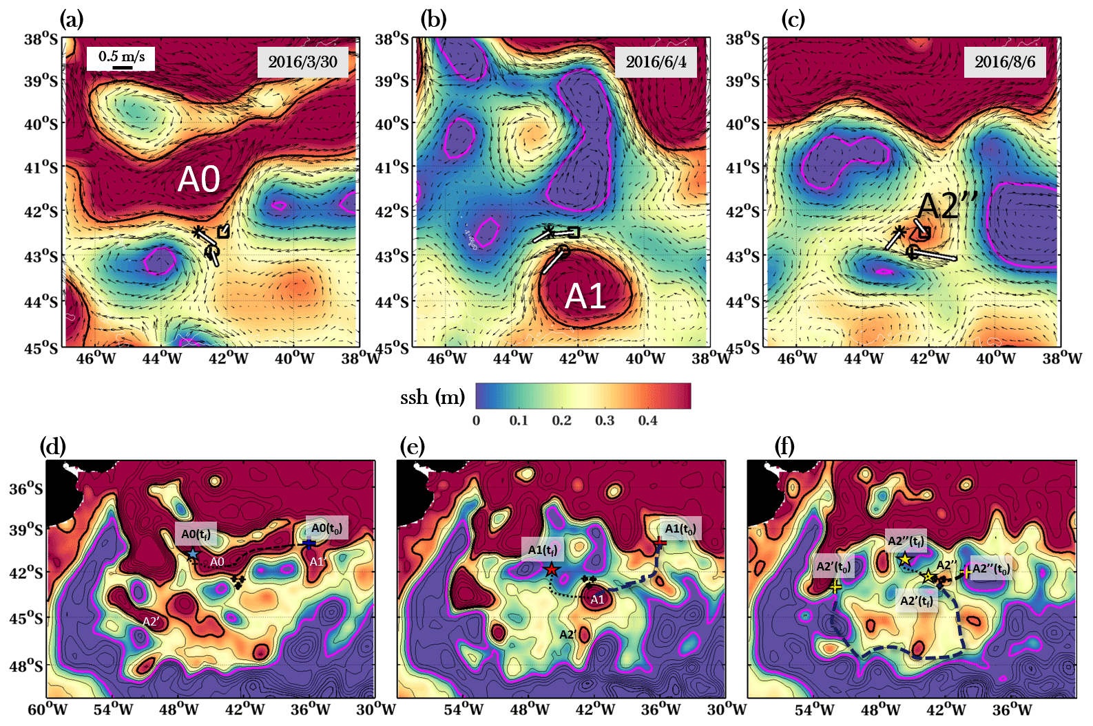
Figure 8 (a–c) SSH (m) and geostrophic velocities (arrows) from satellite altimetry for 30 March, 4 June and 6 August 2016. The vertically integrated in situ velocities are indicated with white arrows. (d–f) SSH over the Argentine Basin at the same dates. Black isolines mark SSH every 0.1 m. The thick black and magenta contours correspond to the STF (SSH = 0.4 m) and the SAF (SSH = 0.05 m). The crosses indicate the region of formation of A0, A1, A2^′ and A2^′′ at time =t₀. The pathway of each structure from its origin to the mooring site (pathway beyond the mooring site) is schematically indicated with dashed (dotted) black curves. The locations where the mesoscale structures are absorbed in the STF at time =t_f are indicated with stars.

The V-shape curvature of the A0 meander boundary near the array on 30 March explains the negative vertically averaged meridional velocities observed at FLMA and SUMO and the positive ones observed at FLMB (Figs. 7d, 8a). FLMA, the closest mooring to the meander, experienced the largest velocities (0.45 m s⁻¹) and dived by 100 m (Appendix A1). The meander had a spatial scale on the order of 600 km and consisted of three anticyclones. The anticyclone in proximity to the mooring array was shed from the STF at 40^∘ S and 36^∘ W on 27 January (blue cross in Fig. 8d). It then re-joined the STF and contributed to the meander (the dashed line in Fig. 8d marks its trajectory). The meander rapidly propagated from 40^∘ S–36^∘ W to the mooring location in 10 d (advection velocity of 0.35 m s⁻¹). The meander broke apart on April 5, and the eddy was absorbed again in the STF on 19 April (at the location marked with the blue star in Fig. 8d).

The large anticyclonic A1 eddy has a radius of about 150 km (Fig. 8b). The moorings sampled the northern part of the eddy (A1) on 4 June and the eastern edge on 15 June (video supplement). The westward displacement of the eddy between the two dates explains the change in sign (from negative to positive) observed in the in situ meridional velocity components (Fig. 7). The eddy is advected with a zonal velocity of 0.15–0.2 m s⁻¹ when passing through the mooring array, while the maximum swirl velocity (estimated from the meridional velocity) is about 0.4 m s⁻¹ (video supplement and Fig. 8b). A1 was shed from the STF at 40^∘ S and 36^∘ W (same location as A0 genesis) on 29 March (red cross in Fig. 8e, animation in video supplement). A1 propagated westward with a speed of about 0.2 m s⁻¹, reaching the mooring array by the beginning of June (Fig. 8e). A1 was absorbed in the STF at the location of the red star in Fig. 8e on 30 June.

In contrast, satellite altimetry suggests that the two anticyclonic eddies contained in event A2 were, small with radii of 20 to 40 and 50 km, respectively. The first eddy (A2^′) reached the mooring array on 15 July after a long journey. Indeed, A2^′ propagated from the Brazil Current domain (43^∘ S–52^∘ W) on 6 March (yellow cross in Fig. 8f and video supplement), was entrained in the Zapiola anticyclonic circulation and reached the mooring array 4 months later. A2^′′ detached from a meander of the STF at 42^∘ S–40^∘ W on 18 July 18 (Fig. 8f) and reached the mooring array on 4 August. Then it propagated northwestward and was absorbed by the STF on 19 September at the location of the yellow star in Fig. 8f.

A0 and A1 were first detected in a region (40^∘ S, 36^∘ W) characterized by a strong gradient in planetary potential vorticity associated with a seamount (Fig. 1a). A1 propagated southward and then westward following the 0.1900 10⁻⁷ $f/H$ contour (Figs. 1b, 8e). A2^′ was advected from the Brazil Current overshoot in the Zapiola anticyclonic circulation along the 0.1925 10⁻⁷ $f/H$ contour (Figs. 1b, 8f).

3.2 Hydrography of the extreme events: A0, A1 and A2

The temperature, salinity and density time series from the discrete unevenly distributed measurement levels were averaged hourly and vertically interpolated (Fig. 9). Event A0, the meander-like structure (Fig. 8a and d), is best documented by FLMB as SUMO was at its periphery and FLMA dived by 100 m. The large A1 eddy (Fig. 8b) is best observed at SUMO as FLMA and FLMB underwent large draw-downs (>400 m) (Fig. A1 in the Appendix, Table 2). In contrast, the A2 event hydrography is rather well documented at the three moorings.

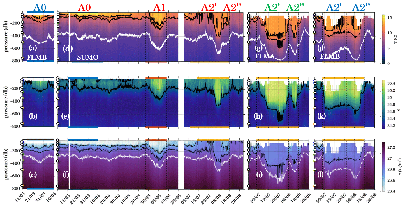
Figure 9 (a–c) Temperature, salinity and density from mooring B (FLMB) during A0 event (hourly averaged data are linearly interpolated in the vertical). In (a), the black isolines are 10^∘C and 12^∘C isotherms, and the white isoline is the 4.5^∘C isotherm. In (b), the black isoline is the 34.5 isohaline. In (c), the black isolines are the 26.65 and 26.85 kg m⁻³ isopycnals, and the white isoline is the 27.00 kg m⁻³ isopycnal. (d–f) Same as (a)–(c) at the surface mooring (SUMO) during events A0, A1 and A2. (g–i) Same as (a)–(c) at mooring A (FLMA) during event A2 event. (j–l) Same as (a)–(c) at mooring B (FLMB) during A2 event. White dots in the y axis indicate the discrete measurement levels.

The A0 event at FLMB (15 March to 10 April) is associated with warm and salty waters (T>8 ^∘C and S>34.15 in the upper 200 m) and depressed isopycnals (down 100 m for isopycnal 27.0 kg m⁻³, reaching 400 m) (Fig. 9a, b, c). The warmest temperatures (17 ^∘C) recorded at SUMO were summer features and were confined to the upper 30 m – these were not sampled by FLMB (Fig. 9d).

In contrast, A1 and A2 events occurred during winter and showed homogeneous waters in the upper layer, which are likely to be associated with winter convection and deep mixed layers (down to 200 m for A1 in June and 350 m for A2^′ in July) (Fig. 9d–l). A1 featured temperatures higher than 8^∘C and salinities larger than 34.15 in the upper 400 m at SUMO (Fig. 9d and e). During A1, isopycnal 27.00 kg m⁻³ deepened down to 500 m. The vertical extension of A1 is at least 1500 m (Fig. 3).

The hydrographic signals associated with A2^′ and A2^′′ are larger at FLMA and FLMB than at SUMO (Figs. 9d–l, 8c, f). SUMO did not sample A2^′ and was on the southern edge of A2^′′. A2^′ signatures are first observed at FLMB between 9 July and 1 August and then at mooring A between 15 July and 5 August (Fig. 9g–l). The displacement of isopycnal 26.86 kg m⁻³ exceeded 300 m at FLMB and 200 m at FLMA. The A2^′ eddy core came closer to FLMA than FLMB as FLMA recorded a thicker homogeneous layer, a larger isopycnal displacement and smaller velocities (Figs. 9g–l and 7a and b). A2^′′ is first observed at FLMB, then at SUMO and lastly at FLMA, with more homogeneous values at FLMB and smaller velocities indicating that the eddy center came closer to FLMB. A2^′ and A2^′′ have vertical extensions of at least 1500 m (Figs. 3 and A1). These large hydrographic vertical extents contrast with the rather small horizontal scales suggested by satellite altimetry.

3.3 Eddy characteristics at the mooring array

The characteristics (SLA amplitude, radius, swirl velocity, lifetime, path length, propagation velocity, intensity, nonlinearity, vertical extension, relative vorticity and Rossby number) of the three vigorous anticyclonic eddies A1, A2^′ and A2^′′ are shown in Table 3. Eddy amplitude is the SLA difference between the eddy center and its periphery. Radius ranges were estimated from the $\mathrm{1}/\mathrm{4}{}^{\circ }$ interpolated satellite-gridded maps in which eddies had an elliptical shape. Therefore, the uncertainty in the radius is reported as a range in Table 3. Intensity is the ratio of the eddy amplitude to its radius (Frenger et al., 2015), and nonlinearity is the ratio of the eddy swirl speed to the propagation velocity (Chelton et al., 2011). Swirl velocities were estimated from in situ and satellite data. They differ by a factor of 2 for A2^′, which was attenuated in satellite altimetry maps. The order of magnitude of the relative vorticity was estimated from in situ swirl velocities and satellite-derived radii. The three anticyclones show distinct characteristics.

Table 3 A1, A2^′ and A2^′′ properties when passing through OOI array.

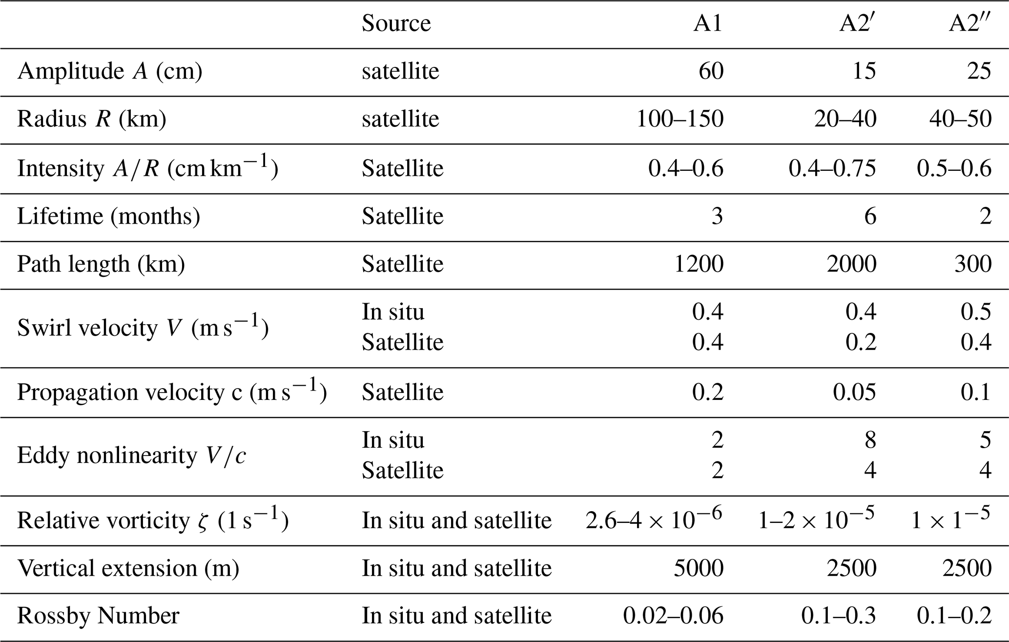
A1 was a large anticyclone (SLA amplitude of 60 cm, radius of 100–150 km and Rossby Number less than 0.1). Event A2 comprised two smaller anticyclones, A2^′ and A2^′′ (amplitudes of 15 and 25 cm, radii of 20–40 and 40–50 km, and 0.1 < Rossby number < 1, respectively). The three eddies A1, A2^′ and A2^′′ were intense (intensities of 0.4–0.5 cm km¹⁻), with similar swirl velocities (about 0.4–0.5 m s⁻¹), and they were nonlinear, advecting trapped fluid and thus transporting water properties (Table 3). A2^′ and A2^′′ underwent winter convection with deep mixed layers in excess of 350 m at FLMA and FLMB.

To estimate the vertical extent of the eddies, we compared time series of dynamic-height anomaly at the mooring sites estimated from the in situ data to the satellite data (Appendix A3). This comparison suggests that A1 was a bottom-reaching structure, while A2^′and A2^′′ extended down to 2500 m at the three moorings.

We now analyze the high-frequency variations associated with the mesoscale structures.

4 High frequencies during extreme events

4.1  Velocity spectral content at high frequencies

Rotary spectra of the ADCP velocities were produced considering 30 d long time series spanning each event, when the moorings did not experience vertical motions. SUMO data were used for the three events (A0, A1 and A2^′′), and FLMB data were used for A0 (Fig. 10). The A2^′ rotary spectra could not be built as the A2^′ event was not sampled at SUMO and induced large vertical displacements in FLMA and FLMB.

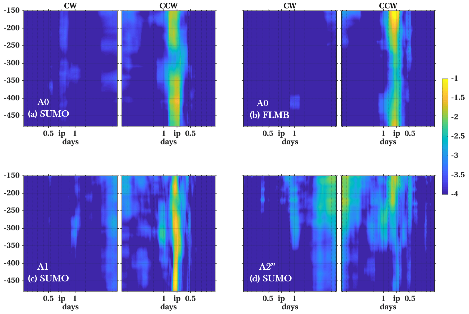
Figure 10 Velocity rotary spectra for A0 event at surface mooring (SUMO) (a), for A0 event at mooring B (FLMB) (b), for A1 event at the surface mooring (c) and for A2^′′ at surface mooring (d). The x axis is periods in days. IP is the inertial period (17 h at the mooring latitude). The y axis is depth in meters. The color bar is log of energy in square meters per second. CW and CCW refer to clockwise and counterclockwise.

All the rotary spectra show a clear peak in energy (of about 0.1 m² s⁻²) near the inertial frequency (period of 17 h at the mooring location) in the counterclockwise motions over the ADCP depth range (down to 480 m). The peaks show a red shift (larger period) relative to the inertial period. The spectra show little (< 0.01 m² s⁻²) or no energy at the diurnal or semi-diurnal period (Fig. 10). The velocity spectra thus indicate prominent motions associated with near-inertial waves (NIW) and negligible tidal currents apart from a low energy signal at middle depth (200–350 m) at the diurnal period of A1 and A2, which could be associated with internal tidal waves around the pycnocline level (Fig. 9d, e and f). SUMO only sampled the A2^′′ boundary. The A2^′′ rotary spectra are blurrier, with energy distributed over a broader band around the inertial period. Energy at a high frequency (period < 17 h) is potentially indicative of cascading energy (Fig. 10d). Event A0 is documented with two spectra (Fig. 10a and b) from SUMO and FLMB ADCP data as FLMA dived by 100 m (Fig. A1 in the Appendix). The peak near the inertial frequency in counterclockwise motions goes through a local minimum around 300–350 m in both spectra. The maximum observed above 200 m in the near inertial frequency band could be associated with locally generated NIWs forced by winds, whereas the local maximum below 350 m may be associated with trapped NIWs (e.g., Martinez-Marrero et al., 2019; Kawagushi et al., 2020).

Theoretical studies have shown that near-inertial waves interact with the vorticity of mesoscale structures and can be trapped by them (Kunze, 1995). The background vertical relative vorticity shifts the inertial frequency (f) to the effective inertial frequency (f_eff) through the zeta-refraction mechanism (e.g., Mooers, 1975; Thomas et al., 2020; Rama et al., 2022): the horizontal velocity shear of anticyclonic eddies ζ shifts f to a lower effective planetary vorticity ($f_{\mathrm{eff}}=f+\mathit{\zeta }/\mathrm{2}$) (Kunze, 1985). In the Southern Hemisphere (f<0), positive ζ values of anticyclonic eddies result in $\left|f_{\mathrm{eff}}\right|<\mid f|$ in their cores. As a consequence of the lowering of $\left|f\right|$ in anticyclonic eddies, the NIWs become superinertial, and their vertical group velocity increases (e.g., Kunze et al., 1995). When NIWs are excited inside a region of anticyclonic relative vorticity, they can have frequencies below f (red shift) and thus remain trapped as they cannot propagate out of the rotating region. As the waves propagate downward from the surface, they reflect off the sides of the anticyclonic region and then stall within a critical layer at the base of the anticyclonic vorticity region, where the group velocity drops to 0. This results in an accumulation of wave energy in a critical layer following tilted isopycnals, and eventually, part of the energy is dissipated by buoyancy release through vertical mixing (e.g., Kunze, 1985; Kunze et al., 1995; Martinez-Marrero et al., 2017; Kawaguchi et al., 2020). Using the ζ values reported in Table 3, f_eff approximately corresponds to a period of about 18 h, consistent with the red shifts observed in Fig. 10 spectra.

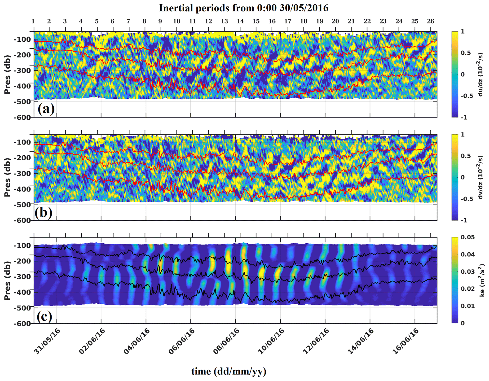
Figure 11 (a–b) Vertical shear of velocity components for SUMO during event A1. (c) The 14–20 h band-pass-filtered kinetic energy for SUMO during event A1. Contours correspond to isopycnals 26.65, 26.85 and 27 kg m⁻³ computed from the vertically interpolated data. Top x ticks indicate inertial periods from 00:00 GMT on 30 May 2016, and bottom x ticks indicate days in dd/mm/yyyy.

As an example of the wave activity, we show the vertical shear of the horizontal velocity components as A1 crosses the SUMO mooring (Fig. 11a and b). The vertical shear features clear wavy patterns close to the inertial period with vertical wavelengths of about 50 m (Fig. 11a and b). The kinetic energy of the band-pass-filtered velocities (14–20 h) shows local maxima along isopycnals 26.65 and 27.00 kg m⁻³ between 1 and 14 June (Fig. 11c). We now examine the occurrence and amplitude of NIW signals in density and velocity shear fields for all the events.

4.2  Near-inertial waves in the density and velocity shear field

We applied a third-order Butterworth band-pass filter around the inertial frequency (14–20 h) to the shear and density time series to isolate the signal associated with the near-inertial waves and computed the envelopes of the filtered signals. Envelopes of the band-pass filter time series measure the amplitude of the fluctuations associated with NIW. The filtered density times series at 180 m for events A0, A1 and A2^′′ at SUMO are shown in Appendix A4 as an example.

During A0, A1 and A2^′′, the shear envelopes show large values at the surface down to 400 m (Fig. 12a). The large shear envelopes at depth occur at times of positive satellite-altimetry-derived $\mathit{\zeta }/f$ (Fig. 12b), confirming that NIWs are trapped in the anticyclonic structures. Note that the temperature at 350 m shows high-frequency variations during the three events (Fig. 12b).

The envelopes of the NIW density signature at each measured level in the upper 500 m at SUMO are shown in Fig. 12c. Large envelope values (> 0.02 kg m⁻³) are observed in the upper 100 m until the end of May when waters are still stratified after austral summer. Local maxima below 150 m extend quite deep in the water column during the three anticyclonic events between isopycnals 26.65 and 27.00 kg m⁻³ (Fig. 12c).

NIWs are generated by a variety of mechanisms, including winds, nonlinear interactions with waves of other frequencies, lee waves over bottom topography and geostrophic adjustment; the partition among these is not known, although the wind is likely the most important (e.g., Alford et al., 2016). The mechanism at the origin of the trapped NIWs at depth was not identified. In particular, the presence of NIWs at depth does not seem to be connected with strong wind episodes at the OOI (Fig. 12d).

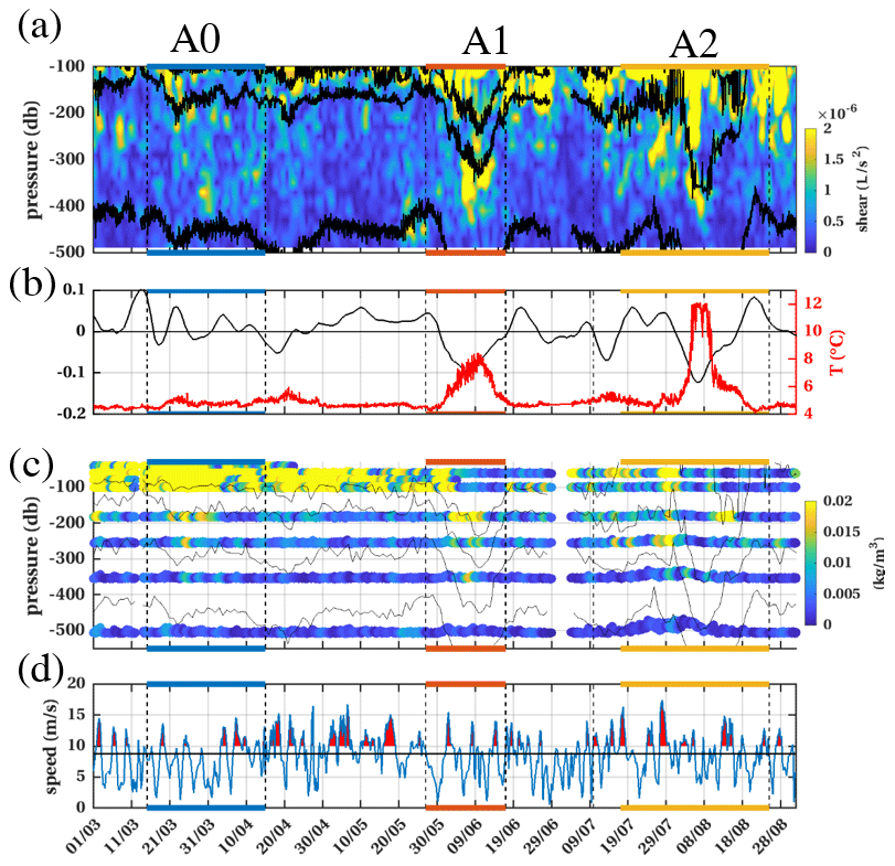
Figure 12 (a) Envelope of the 14–20 h band-pass-filtered shear intensity at SUMO. Black isolines are three isopycnals computed from SUMO vertically interpolated density time series, namely 26.65, 26.85 and 27.00 kg m⁻³. (b) Satellite-altimetry-derived $\mathit{\zeta }/f$ (left y axis) and temperature at 350 m at SUMO (right y axis). (c) Envelope of the 14–20 h band-pass-filtered density at SUMO. (d) Wind intensity from Era-Interim at SUMO. Red colors indicate values larger than 10 m s⁻¹.

The energy from the trapped waves must then be transferred to smaller waves, which eventually break, generating turbulence and mixing (Kunze et al., 1995). The tendency of a stratified water column to become unstable can be estimated with the Richardson number $\mathit{Ri}=N^{\mathrm{2}}/S^{\mathrm{2}}$, where N² is the Brunt–Väisälä frequency and S² is the squared velocity shear ($S^{\mathrm{2}}=(\partial u/\partial z{)}^{\mathrm{2}}+(\partial v/\partial z{)}^{\mathrm{2}}$). The Richardson number is often used as a proxy to predict the likelihood of overturning events and enhanced mixing in a stratified fluid due to shear instability acting against the stable buoyancy field. Though the existence of a universal critical Richardson number Ri_c at which turbulent mixing can start is still debated, a lower-bound Ri<Ri_c is often assumed – for example, ${\mathit{Ri}}_{\mathrm{c}}=\mathrm{1}/\mathrm{4}$, originally derived from the linear stability of steady stratified shear flows (Miles, 1961), or Ri_c=1 from nonlinear stability analysis (e.g Abarbanel et al., 1984).

4.3 Richardson number

The Brunt–Väisälä frequency (Fig. 13, first row) was estimated from interpolated densities shown in Fig. 9 (only seven to eight measurement levels). A Richardson number (Fig. 13, last row) was tentatively computed as the daily minimum of the ratio between N² and the squared amplitude of the vertical shear of the horizontal velocity (Fig. 13, second row).

The A0 event (15 March to 10 April), best appreciated at FLMB (Fig. 13a, b, c) with a larger depression of the 27.00 kg m⁻³ isopycnal than at SUMO, is associated with rather large N² values compared to the surrounding waters (Fig. 13a). The velocity shear amplitude features large values in the upper stratified 150 m and, interestingly, a local maximum below the 27.00 kg m⁻³ isopycnal at its deepest level (400 m), resulting in a rather small Richardson number (0.75) (Fig. 13b and c).

A1 is sampled in austral fall (end of May to beginning of June) and features low N² (less than $\mathrm{0.1}\times {\mathrm{10}}^{-\mathrm{5}}$ s⁻² in the upper 200 m) on 9 June, when isopycnals reach their maximum depth (Fig. 13d). Below this homogeneous upper core, SUMO documented stratified waters with large N² values ($N^{\mathrm{2}}>\mathrm{2.5}\times {\mathrm{10}}^{-\mathrm{5}}$ s⁻²), a local maximum in the shear intensity around isopycnal 27.00 kg m⁻³ (when deeper than 300 m) ($\mathrm{4}\times {\mathrm{10}}^{-\mathrm{5}}$ s⁻²), that led to a Richardson number of about 0.62 (Fig. 13d, e, f). A strikingly low Richardson number (Ri=0.32 from 20 to 30 May) is observed at depth (below 400 m) just before the A1 event and corresponds to a vigorous velocity vertical shear at a time of steeply shallowing isopycnals (Fig. 13f).

Anticyclones A2^′ and A2^′′ have a deep-reaching (350 m at FLMB and 250 m at FLMA) homogeneous layer of low N² ($N^{\mathrm{2}}<\mathrm{0.5}\times {\mathrm{10}}^{-\mathrm{5}}$ s⁻²) corresponding to deep winter mixed layers (Fig. 13g and j). Below the homogeneous mixed layer, a local maximum of N² on the order of $\mathrm{1.5}\times {\mathrm{10}}^{-\mathrm{5}}$ s⁻² is centered around the 26.85 kg m⁻³ isopycnal. The velocity shear S² is small in the mixed layer and increases below the 27.0 kg m⁻³ isopycnal (Fig. 13h and k). The Richardson number estimates show two minima in the vertical: one in the deep winter mixed layer, dominated by extremely small N², and another one below the 27.0 kg m⁻³ isopycnal, where velocity shear is important (Ri of about 0.6 to 0.7) (Fig. 13g, h, i, j, k and l). The two minima are separated by a layer of large Ri (3.16), which corresponds to N² values of $\mathrm{1.5}\times {\mathrm{10}}^{-\mathrm{5}}$ s⁻².

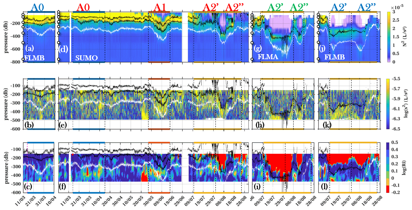
Figure 13 (a–c) Brunt–Väisälä frequency (N²) (hourly averaged data are linearly interpolated in the vertical), amplitude of vertical shear and Richardson number during event A0 at mooring B. The Richardson number was tentatively computed as the daily minimum of the ratio between N² and the vertical shear of the horizontal velocity. The black isolines are the 26.65 and 26.85 kg m⁻³ isopycnals, and the white isoline is the 27.00 kg m⁻³, isopycnal which corresponds to the limit between SACW and AAIW. White dots in the y axis in (a) indicate the discrete measurement levels. (d–f) Same as (a)–(c) at the surface mooring during events A0, A1 and A2. (g–i) Same as (a)–(c) at mooring A during event A2 event. (j–l) Same as (a)–(c) at mooring B during A2 event.

The Richardson number has been considered as a valuable proxy for turbulence production in the oceans, and the presence of low, fine-scale Ri associated with internal waves (NIWs) has been frequently observed in the ocean interior (e.g., Martinez Marrero, 2019). In these studies, it was assumed that shear occurring at scales beyond the resolution of the ADCP would sufficiently reduce the total Richardson number to trigger shear instability. The Ri estimates, based on a relatively coarse vertical resolution of N² and S², show low values close to 1 in the specific regions where trapped NIWs were detected: the four anticyclonic features show a low Ri at depth (between 300 and 400 m for A0 and A1 and between 400 and 500 m for A2^′ and A2^′′) at the limit between SACW and AAIW (indicated with a white isoline in Fig. 13). The low Ri estimates suggest that favorable conditions for enhanced mixing between AAIW and SACW occurred at depth within the anticyclones where NIWs are trapped and eventually break.

5 Summary and conclusions

We analysed physical parameters recorded by the OOI mooring array deployed at 42.5^∘ S and 42.5^∘ W, a remote site in the data-sparse Argentine Basin. The moorings were located 3^∘ to the south of the Subtropical Front mean position and to the north of the Zapiola anticyclone in a region characterized by rough weather conditions and relatively low EKE ($\mathrm{145}\times {\mathrm{10}}^{-\mathrm{4}}$ m² s⁻²) compared to the surroundings (EKE can be as large as $\mathrm{1000}\times {\mathrm{10}}^{-\mathrm{4}}$ m² s⁻² in the Brazil Malvinas Confluence) (Fig. 1).

Year 2016 stands out with a maximum of EKE (> $\mathrm{1000}\times {\mathrm{10}}^{-\mathrm{4}}$ m² s⁻²) in the 29-year-long satellite altimetry record at the mooring site. We investigated possible circumstances (ocean circulation, wind anomalies) leading to this unique EKE peak in 2016 without any conclusive results. This needs further investigation. The mooring array documented four exceptional events in 2016. We tentatively address the questions raised in the introduction.

What are these extreme events? The four events were anticyclonic structures, a meander of the Subtropical Front (A0) and three intense anticyclonic eddies with swirl velocities on the order of 0.4 m s⁻¹. Satellite altimetry provided information on the size, origin and fate of the structures. The three anticyclonic eddies (named A1, A2^′ and A2^′′) showed distinct characteristics. A1 was a large, 200–300 km diameter, bottom-reaching eddy (bottom > 5000 m). In contrast, A2^′ and A2^′′ were smaller and attenuated in the satellite altimetry maps. They had radii of about 40 km, with that of A2^′ probably being smaller and that of A2^′′ being slightly larger, and a vertical extent of about 2500 m. In the region, the baroclinic Rossby radius is ∼ 25 km (Chelton et al., 1998).

Where do those anticyclonic structures come from? Satellite altimetry suggested that the three eddies had different origins and paths. A1 detached from the STF 600 km to the northeast of the array over a topographic rise (40^∘ S, 36^∘ W) 60 d before crossing the OOI array. A2^′ was tracked back as a large anticyclonic eddy detached from the Brazil Current overshoot (43^∘ S, 52^∘ W). It traveled for 4 months with the Zapiola anticyclonic circulation before reaching the array. While at the array, satellite altimetry maps suggest that A2^′ merged with A2^′′, which arrived after a 16 d trip from its first-detected place at 42^∘ S, 40^∘ W. After a lifetime of 3, 6 and 2 months for A1, A2^′ and A2^′′, respectively, the three eddies were reabsorbed by the STF.

How often do the extreme events occur? The altimetry-derived EKE time series at the mooring location showed that those events were exceptional (Fig. 6). Other less extreme anticyclonic eddies crossed OOI moorings; they are seen as peaks in OOI hydrographic data and EKE time series. Energetic eddies detached from the subtropical front are frequent in the Argentine Basin (Fig. 1), in particular in the Brazil–Malvinas Confluence, in the vicinity of the STF and in a band centered at 49^∘ S (e.g., Fu, 2006; Mason et al., 2017; Artana et al., 2019). Thus, OOI observations in 2016 are relevant and valuable for the data-sparse Argentine Basin.

Do the anticyclonic structures documented with OOI impact mixing? These anticyclonic structures are not subtropical run-away eddies lost to the subantarctic waters; they were reabsorbed in the subtropical waters. The mooring data provided evidence of favorable conditions for the potential development of mixing well below the mixed layer. Indeed, tentatively estimated Richardson numbers showed two minima in the vertical during the extreme events, one in the mixed layer and another one below the mixed layer depth at the 27.00 kg m⁻³ horizon associated with NIWs, suggesting mixing between the SACW and the AAIW. Regardless of their size and origin, the four anticyclonic structures presented low Ri associated with trapped NIWs, suggesting that enhanced mixing at depth is probably found in the many anticyclonic eddies populating the Argentine Basin. Those numerous anticyclonic mesoscale eddies likely act as mixing structures at the pycnocline and bring heat and salt from the SACW to the AAIW, and they are certainly relevant in modifying the upper-water-mass characteristics in the Argentine Basin.

The OOI array provided unprecedented long time series with a high temporal sampling in the Southern Hemisphere and, for the first time, documented near-inertial waves trapped at depth within anticyclones in the Argentine Basin. The majority of observational evidence of NIW trapping in anticyclonic structures is from the Northern Hemisphere and relies upon quasi-synoptic continuous vertical density profiles, allowing estimates of NIW vertical scales, small structures in the Brunt–Väisälä frequency and dissipation rates (e.g., Joyce et al., 2013; Karstensen et al., 2017; Martinez-Marrero et al., 2019), and recently upon mooring data (e.g., Kawaguchi et al., 2020, 2021; Xu et al., 2022; Yu et al., 2022; Ma et al., 2022).

Precise examination of NIWs is beyond the scope of this work and deserves further investigation. Recent analyses of mooring observations in the Northern Hemisphere have provided new insights into NIWs trapped in anticyclonic eddies. Kawaguchi et al. (2020) highlighted trapped amplified NIWs with multiple inertial frequencies (double, triple and quadruple) generated by a fast-moving cyclone (winds > 20 m s⁻¹) passing over an anticyclone in the central Sea of Japan. The OOI array did not detect multiple inertial frequencies in the anticyclones. In the northern South China Sea, Xu et al. (2022) evidenced an anticyclonic eddy carrying typhoon-generated trapped NIWs for at least 660 km and 79 d. Wind episodes leading to the NIW generation in the anticyclones observed at OOI were not clearly identified. ERA-Interim winds showed various strong wind events (wind speed larger than 20 m s⁻¹) along the eddy paths. NIW penetration down to 1400 m close to the seabed was observed in the northwestern South China Sea (Ma et al., 2022). The vertical range of the OOI ADCP data prevented the examination of the presence of NIW below 500 m, and the vertical extent of the NIW penetration is an open question as A1 was a bottom-reaching eddy and A2^′ and A2^′′ had a vertical extension of 2500 m. Kawaguchi et al. (2021) documented amplified signals of NIW-related vertical shear and turbulent kinetic energy dissipation between cores of pair vortices (adjacent cyclone and anticyclone). A strikingly low Ri was observed at depth below 400 m just before the A1 event at SUMO. The low Ri values are found between eddy cores of a tripole structure crossing the mooring array (not shown). Further investigation is needed to prove the link between the tripole and the low Ri values. Mooring observations at a submesoscale sampling in the northeast Atlantic, a region with moderate EKE, suggested that submesoscale motions with Rossby numbers close to 1 are limited to the mixed layer and have little effect on the trapping and vertical penetration of NIWs (Yu et al., 2022). The OOI eddies have Rossby numbers between 0.01 and 0.6, and A2^′, blurred in the satellite altimetry maps, could be considered to be a submesoscale feature. The interactions between submesoscale features and NIWs could be different in a highly energetic region like the Argentine Basin, where submesoscale motions are possibly not limited to the mixed layer.

Appendix A

A1  Hydrography at FLMA, FLMB and APEX

FLMA and FLMB did not move much during deployments 1 and 3, while they underwent large draw-downs during deployment 2 (Fig. A1). The A0 event led to vertical excursions of 100 m at 1500 m depth at FLMA, while FLMB remained still (Fig. A1). As a result, the A0 event signed with temperature and salinity maxima in the FLMB time series and minima in the time series in the upper layer of the blown-down FLMA (Fig. A1).

Event A1 led to vertical excursions in excess of 400 m at FLMA and FLMB and to the collapse of the APEX profiler in May 2016 (Fig. A1c, f, g and h). As a result of the draw-downs, the temperature (salinity) time series at FLMA and FLMB feature a local minimum in the upper 1000 m (250 m) during A1 instead of a maximum, as in SUMO (Figs. A1 and 3). In contrast, FLMA and FLMB, which did not dive, recorded local maxima in temperature and salinity (down to 1500 m in temperature and 500 m in salinity) (Fig. A1).

The APEX profiler data with a continuous vertical resolution of about 2 m between 250 to 1500 m clearly show the limits of the Antarctic Intermediate Water between 250 and 750 m (salinity minimum) and the Upper Circumpolar Deep Water below (Fig. A1). The APEX mooring did not sample A1 and A2 events due to its collapse.

A2 Horizontal velocity statistics

A3 Vertical extent of the eddies

To estimate the vertical extent of the eddies, we compared time series of dynamic-height anomalies at the mooring sites estimated from the in situ data to the satellite data (Fig. A2). As the mooring data suggest that the three eddies were structures reaching below 1500 m (Sect. 3.2), we tentatively complemented the hydrographic mooring data below 1500 m with the CTD data of the deployment cruise. Various reference levels were considered in the estimation of the dynamic-height anomaly.

The dynamic-height anomaly computed using a 5000 m reference level is well matched (RMSD 9 cm) to the along-track SLA during event A1 at the SUMO location, suggesting that A1 was a bottom-reaching structure (Fig. A2b). In contrast, the best match between the different dynamic heights and the along-track SLA during A2^′ and A2^′′ is found with a reference level of 2500 m at the three moorings (RMSD of 10 cm at SUMO, 15 cm at FLMA and FLMB), suggesting that both structures were shallower than A1 (Fig. A2b, c, d).

A4 Density envelopes

We applied a third-order Butterworth band-pass filter around the inertial frequency (14–20 h) to the density time series to isolate the density signal associated with the near-inertial waves and computed the envelopes of the filtered signals. The filtered density times series at 180 m for events A0, A1 and A2 at SUMO are shown as an example (Fig. A3). Density was available at discrete, unevenly distributed depths. Stratification was tentatively estimated with the Brunt–Väisälä frequency ($N^{\mathrm{2}}=-g/\mathit{\sigma }\partial \mathit{\sigma }/\partial z$) calculated from the vertically interpolated temperature and salinity time series. Envelopes of the band-pass-filtered density time series measure the amplitude of the density fluctuations associated with NIW (red curves in Fig. A3a–c). The filtered density time series tend to show larger amplitude variations when stratification increases (N² above $\mathrm{1.5}\times {\mathrm{10}}^{-\mathrm{5}}$ S⁻²) and smaller ones when stratification is weak. This is particularly striking during the A2^′′ event: when N² is close to zero from 4 to 10 August, the NIW signal in density reduces to less than 0.01 kg m⁻³, and it increases to 0.4 kg m⁻³ when N² exceeds $\mathrm{3}\times {\mathrm{10}}^{-\mathrm{5}}$ from 15 to 17 April (Fig. A3c).

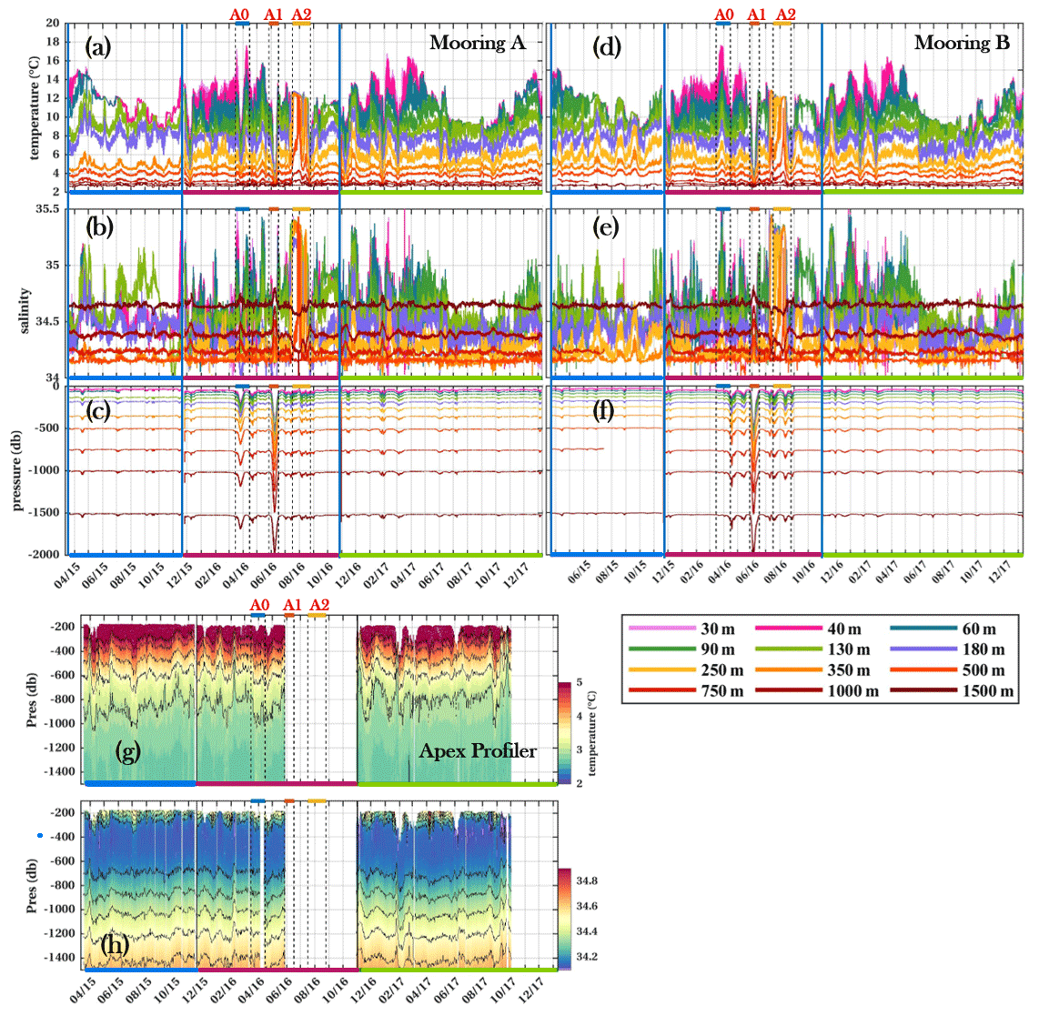
Figure A1 Temperature (a, d, g), salinity (b, e, h) and pressure (c, f) time series at different depths (indicated with colors) from moorings A and B and the APEX profiler mooring instruments. Three events are labeled: A0, A1 and A2.

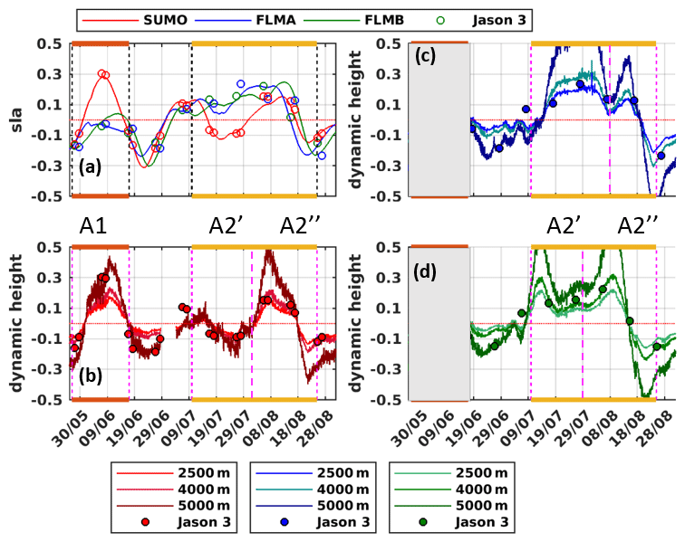
Figure A2 (a) SLA time series from satellite altimetric maps (full lines) and Jason-3 satellite tracks (circles) interpolated at the mooring location (SUMO in red, FLMA in blue and FLMB in green). (b) Dynamic-height anomaly computed from vertically interpolated temperature and salinity, referring to 2500, 4000 and 5000 m for SUMO and SLA from Jason at the mooring location. (c) Same as (b) for FLMA. (d) Same as (b) for FLMB. Shaded areas in (c) and (d) correspond to severe draw-down during A1. The mean between the period of 26 May to 1 September was removed to obtain the SLA and the dynamic-height anomaly.

Table A1 Horizontal velocity statistics: mean (μ), standard deviation (σ, in 10⁻² m s⁻¹) and EKE (in 10⁻⁴ m² s⁻²). In situ velocities were vertically averaged. Vertical averages cover the depth range 150–450 m for SUMO and variable depth ranges for FLMA and FLMB because of the vertical excursions. SGV stands for daily altimetry-derived surface geostrophic velocity.

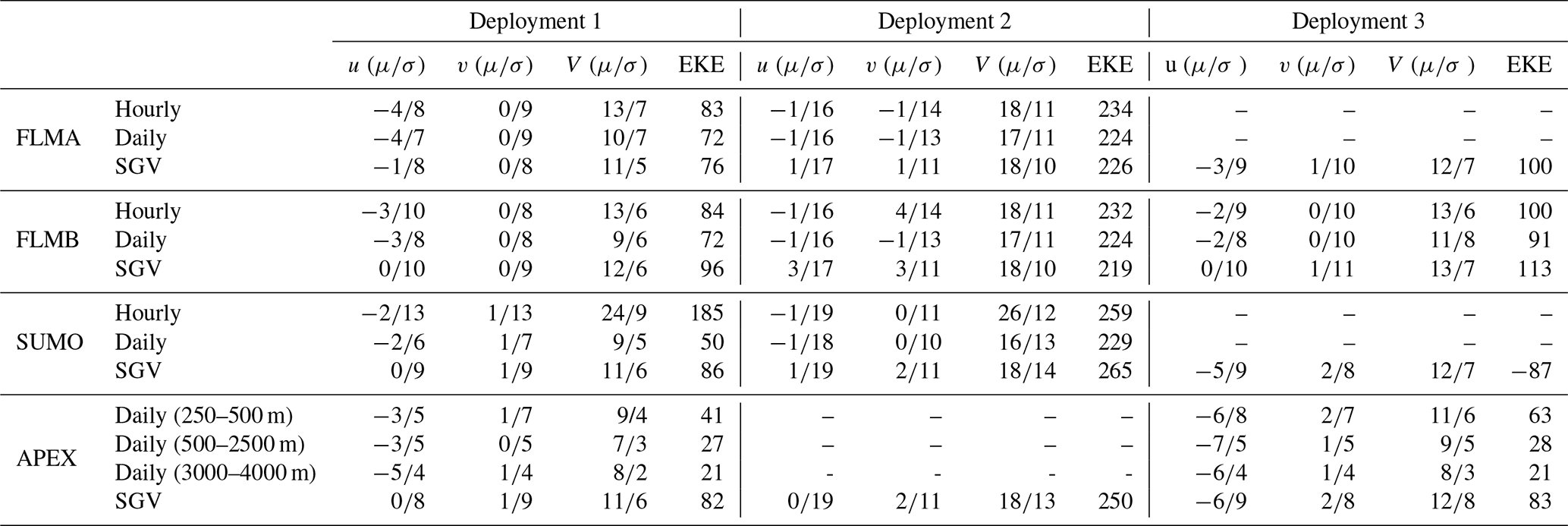
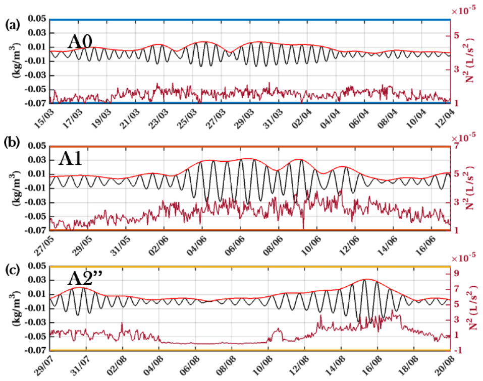
Figure A3 (a–c) The (14–20 h) band-pass-filtered density time series (in kilograms per cubic meter) at 180 m (black), the envelope of the filtered signal in red (left axis) and the Brunt–Väisälä frequency time series at 180 m in brown (right axis) for events A0 (a), A1 (b) and A2 (c) from SUMO.