the Creative Commons Attribution 4.0 License.
the Creative Commons Attribution 4.0 License.
 | 18 Jan 2023
River effects on sea-level rise in the Río de la Plata estuary during the past century
Identifying the causes for historical sea-level changes in coastal tide-gauge records is important for constraining oceanographic, geologic, and climatic processes. The Río de la Plata estuary in South America features the longest tide-gauge records in the South Atlantic. Despite the relevance of these data for large-scale circulation and climate studies, the mechanisms underlying relative sea-level changes in this region during the past century have not been firmly established. I study annual data from tide gauges in the Río de la Plata and stream gauges along the Río Paraná and Río Uruguay to establish relationships between river streamflow and sea level over 1931–2014. Regression analysis suggests that streamflow explains 59 %±17 % of the total sea-level variance at Buenos Aires, Argentina, and 28 %±21 % at Montevideo, Uruguay (95 % confidence intervals). A long-term streamflow increase effected sea-level trends of 0.71±0.35 mm yr−1 at Buenos Aires and 0.48±0.38 mm yr−1 at Montevideo. More generally, sea level at Buenos Aires and Montevideo respectively rises by m and m per 1 m3 s−1 streamflow increase. These observational results are consistent with simple theories for the coastal sea-level response to streamflow forcing, suggesting a causal relationship between streamflow and sea level mediated by ocean dynamics. Findings advance understanding of local, regional, and global sea-level changes; clarify sea-level physics; inform future projections of coastal sea level and the interpretation of satellite data and proxy reconstructions; and highlight future research directions. Specifically, local and regional river effects should be accounted for in basin-scale and global mean sea-level budgets as well as reconstructions based on sparse tide-gauge records.
- Article
(7603 KB) - Full-text XML
- BibTeX
- EndNote


Tide-gauge records of relative sea level go back more than a century in some places, representing some of the longest instrumental time series of the Earth system (Hogarth, 2014; Talke et al., 2018; Woodworth et al., 2010). On long climate timescales, changes in global mean sea level are informative of global ocean warming, land ice wastage, and terrestrial water storage, whereas local and regional deviations from the global average shed light on processes including ocean dynamics and gravitation, rotation, and solid Earth deformation (Gregory et al., 2019; Horton et al., 2018; Kopp et al., 2015). Identifying the mechanisms responsible for sea-level changes observed in tide-gauge records is therefore a major goal in geophysics, oceanography, and climate science (Douglas et al., 2001; Emery and Aubrey, 1991; Lisitzin, 1974).
The nature and causes of twentieth-century sea-level changes in the South Atlantic Ocean are poorly understood compared to behavior in other ocean basins during the same time period (Dangendorf et al., 2017; Frederikse et al., 2018). This knowledge gap reflects a lack of data – the basin has few long tide-gauge records (Hamlington and Thompson, 2015; Natarov et al., 2017). Given the basin's large area (Thompson and Merrifield, 2014), the absence of long data records in the South Atlantic Ocean poses a particular challenge for estimates of global mean sea-level rise (Church and White, 2011; Dangendorf et al., 2017; Frederikse et al., 2020; Hay et al., 2015; Jevrejeva et al., 2014; Ray and Douglas, 2011), but also for our understanding of circulation and climate during the past century more generally.
A recent study brings together available tide-gauge records along with other data, proxies, and models to quantify rates and mechanisms of twentieth-century South Atlantic sea-level change (Frederikse et al., 2021). Those authors determine that sea level in the South Atlantic rose about 0.3 mm yr−1 faster than the rate of global mean sea-level rise owing to a combination of ocean dynamics and gravitational, rotational, and deformational effects from contemporary mass redistribution. Importantly, their estimate of twentieth-century sea-level rise over the South Atlantic rests heavily on a handful of long tide-gauge records in and around the Río de la Plata, which feature large sea-level trends that have been reported on previously (Aubrey et al., 1988; Brandani et al., 1985; D'Onofrio et al., 2008; Dennis et al., 1995; Douglas, 1997, 2001, 2008; Emery and Aubrey, 1991; Fiore et al., 2009; Isla, 2008; Lanfredi et al., 1988, 1998; Melini et al., 2004; Pousa et al., 2007; Verocai et al., 2016).
The Río de la Plata is a long, broad, shallow salt-wedge estuary that widens from ∼50 to ∼250 km and deepens from ∼5 to ∼20 m between Buenos Aires, Argentina, and Punta del Este, Uruguay, before emptying out onto the shelf (Guerrero et al., 1997; Verocai et al., 2016; Figs. 1, 2). The estuary is typified by a strong salinity and turbidity front at Barra del Indio Shoal between Punta Piedras, Argentina, and Montevideo, Uruguay, with fresher, more turbid waters upstream to the northwest, and saltier, less turbid waters downstream to the southeast (Acha et al., 2018; Guerrero et al., 1997; Moreira and Simionato, 2019). These features, and the region's hydrography and ecology generally, are strongly shaped by the situation of the estuary at the confluence of the Río Paraná and Río Uruguay, which are two of the world's largest rivers by streamflow and drainage.
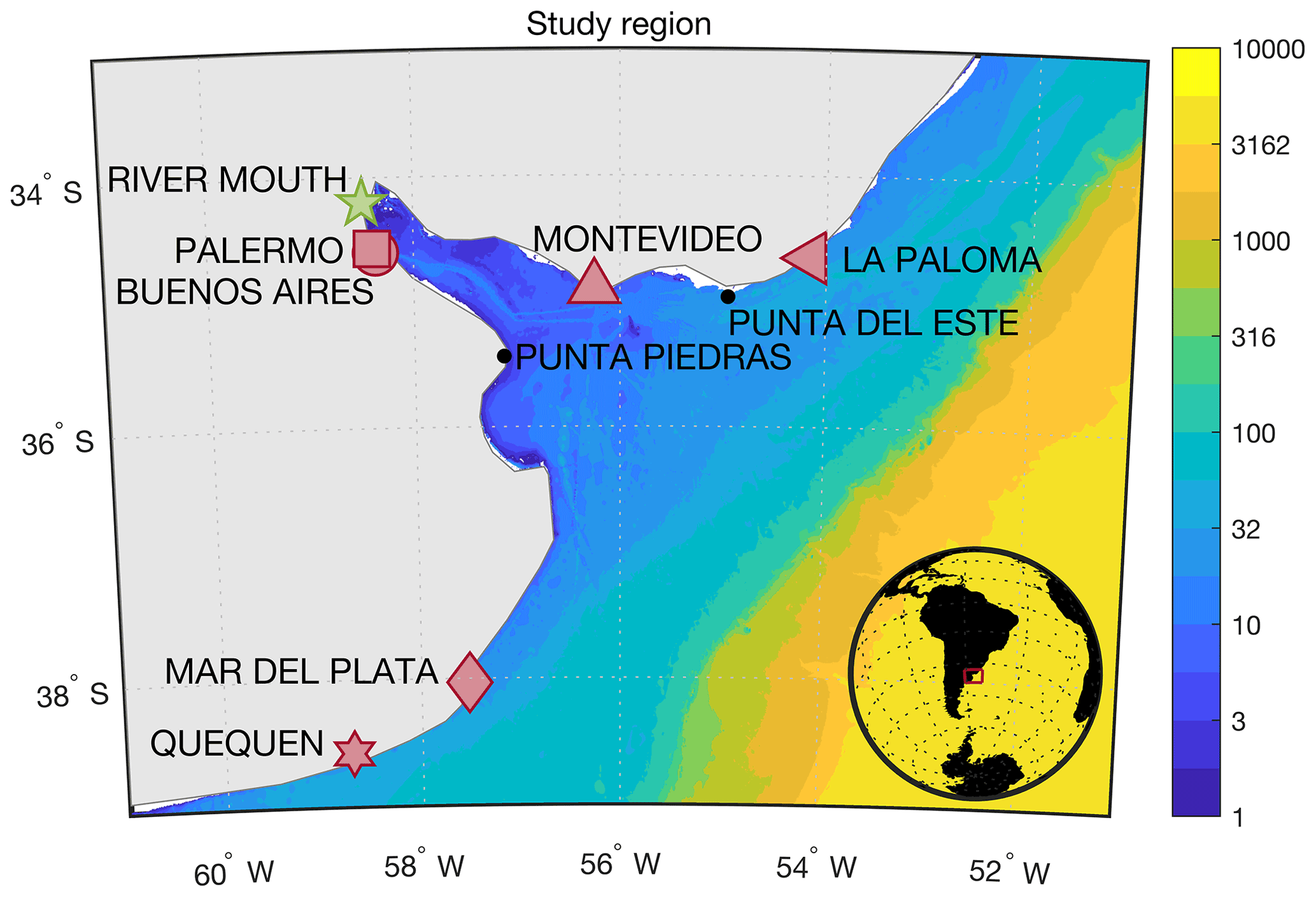
Figure 1Study region. Color shading is bathymetry (m) from the GEBCO 2021 grid (GEBCO Compilation Group, 2021). Note the nonlinear color scale. Red symbols locate tide gauges. The green star is the river mouth, selected as the confluence of the Río Paraná and Río Uruguay near Isla Oyarvide. Black dots identify other locations referenced in the text. The inset shows the study area in a global context.
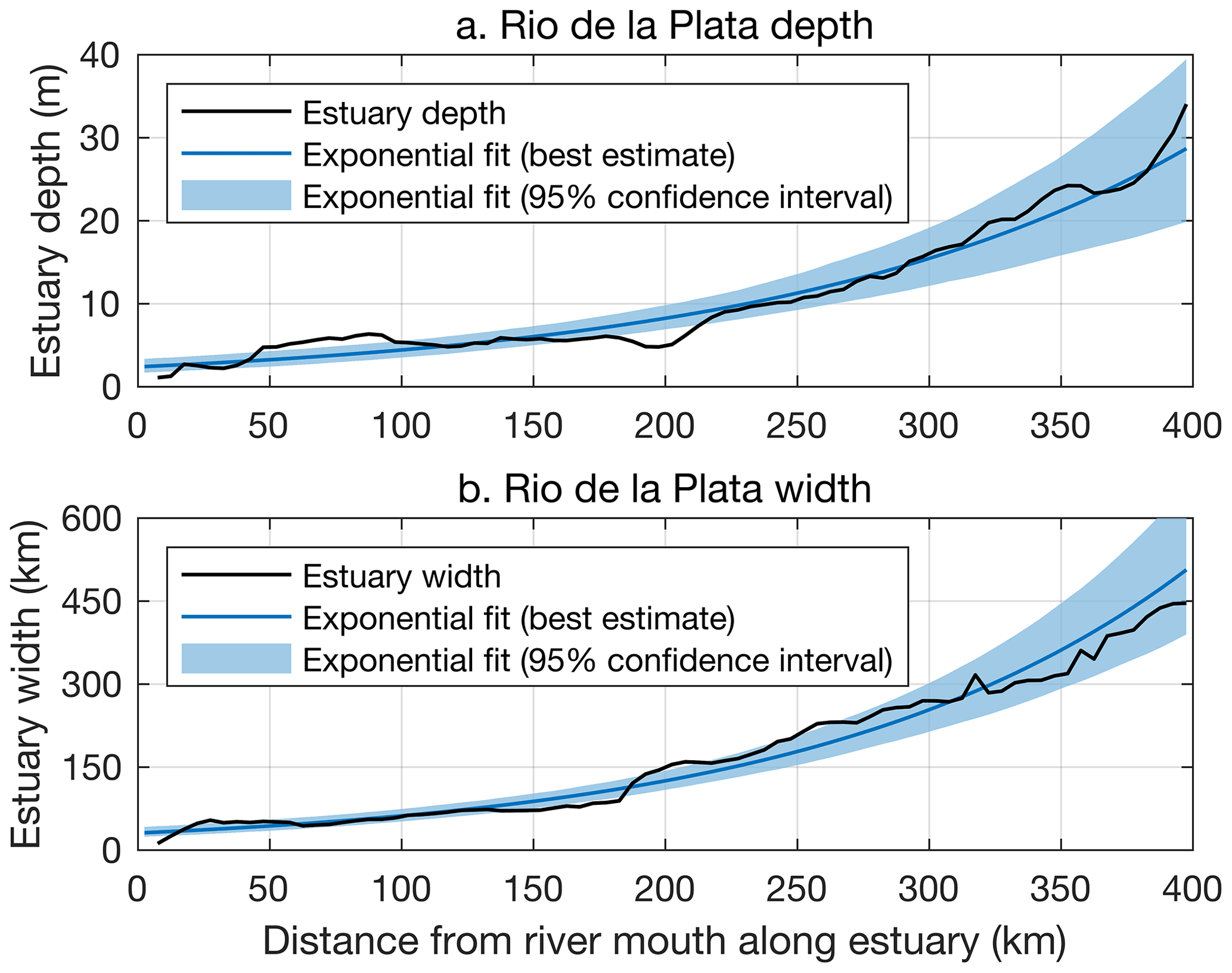
Figure 2Black curves illustrate the (a) average depth and (b) width of the Río de la Plata as a function of distance along the estuary from the river mouth based on the GEBCO 2021 grid (GEBCO Compilation Group, 2021). Values are determined by identifying all marine grid cells (depths <0) in successive 5 km increments from the river mouth. The average depth is computed as the arithmetic mean of all grid cell depths, and the width is defined as the maximum distance between the marine grid cells within the given 5 km increment. Dark blue curves and light blue shading represent best estimates and 95 % confidence intervals, respectively, of exponentials fit to the black curves using ordinary least squares. To account for residual autocorrelation, the uncertainties are based on the effective degrees of freedom assuming residuals are described by an order-1 autoregressive model.
Streamflow into the Río de la Plata increased over the past century (Dai, 2016; Dai and Trenberth, 2002; Dai et al., 2009; see Fig. 3). However, the possible influence of the increased streamflow on multidecadal and centennial sea-level trends has not been considered. Discussions of the connection between streamflow and regional sea level are mostly qualitative and center on interannual variability at Buenos Aires in relation to El Niño; for example, precipitation over the Plata Basin, streamflow of the Río Paraná and Río Uruguay, and sea level at Buenos Aires tend to increase in succession during El Niño events (Douglas, 2001; Frederikse et al., 2021; Isla, 2008; Meccia et al., 2009; Papadopoulous and Tsimplis, 2006; Raicich, 2008; Santamaria-Aguilar et al., 2017; Thompson et al., 2016; Verocai et al., 2016). Douglas (2001) and Thompson et al. (2016) argue that sea-level trends calculated from the Buenos Aires tide gauge are effected by sea-level variability during the 1982–1983 El Niño. While both studies relate this variability to river effects, Douglas (2001) favors an interpretation in terms of ocean dynamics, whereas Thompson et al. (2016) appeal to gravitational, rotational, and deformational effects. Aubrey et al. (1988) and Melini et al. (2004) give alternative interpretations of regional tide-gauge trends generally in terms of continental crustal rifting as well as subsidence and the sea-level response to the 1960 Valdivia earthquake, respectively. Therefore, it remains unclear what processes mediate the relationship between streamflow and sea level, how these two variables are related more broadly as a function of time, and whether such considerations are relevant for interpreting long-term sea-level trends. A dedicated comparison of long stream- and tide-gauge records that provides a physical interpretation and establishes causality is needed.
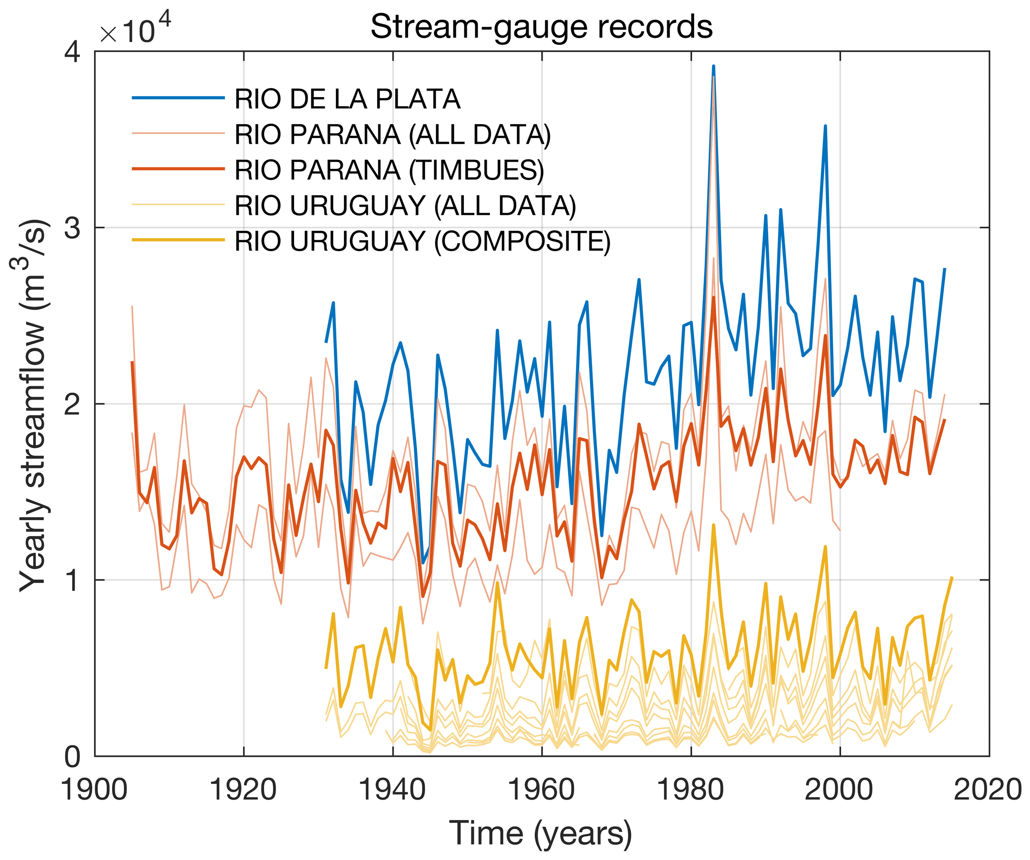
Figure 3Yearly river-gauge streamflow records (Table 1). The thick blue Río de la Plata time series is the sum of the thick red Río Paraná time series from Timbúes and the thick yellow composite Río Uruguay time series. Thin time series show data from individual gauges.
Did streamflow effect long-term sea-level trends at tide gauges in the Río de la Plata? If so, what processes were involved? To answer these questions, I apply statistical analyses to annual data from stream gauges and tide gauges over the past century, and I formulate simple theories based on ocean dynamics to interpret the results. I conclude that local estuarine and coastal ocean dynamics forced by changes in streamflow had an important impact on twentieth-century sea-level rise in the Río de la Plata. Once adjusted for these effects and background late Holocene rates, both of which contribute negligibly to changes in global ocean water volume, the tide gauges show trends more in line with contemporary estimates of twentieth-century global mean sea-level rise (Dangendorf et al., 2017; Frederikse et al., 2020; Hay et al., 2015). The remainder of this paper is structured as follows: in Sect. 2, I describe the datasets; I report on results of the observational analysis, which involves correlation and regression methods applied to the data, in Sect. 3; in Sect. 4, I develop simple analytical models of the sea-level response to streamflow forcing to interpret observational results from Sect. 3; finally, I conclude with a summary and discussion in Sect. 5.
2.1 Streamflow
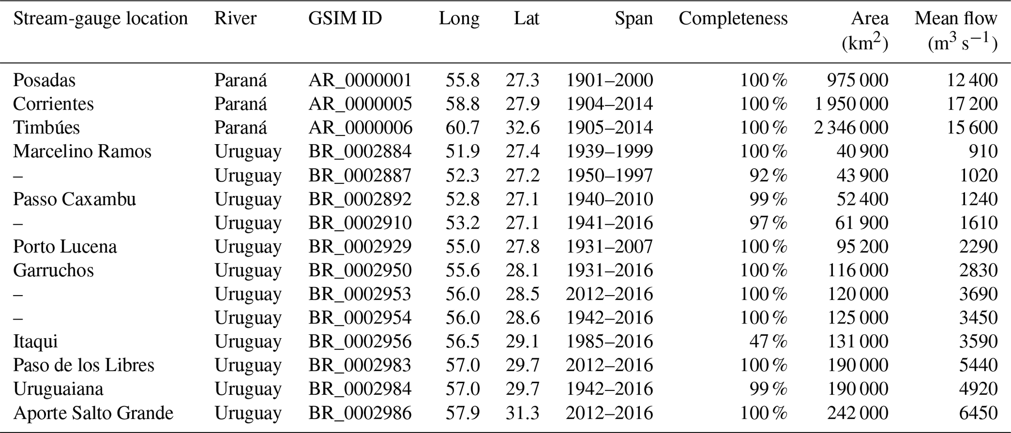
I use yearly streamflow records from the Global Streamflow Indices and Metadata Archive (GSIM; Do et al., 2018; Gudmundsson et al., 2018a). The GSIM database gives data from 3 stream gauges along the Río Paraná and 12 from the Río Uruguay (Table 1; Fig. 3). To estimate Río de la Plata streamflow, I combine data from the two rivers. Records from the Río Paraná are long and complete. Therefore, I use the time series from Timbúes, which spans 1905–2014 and has the largest gauged area. Data from the Río Uruguay are shorter and more gappy; for example, the station with the largest drainage, Aporte Salto Grande, only gives data for 2012–2016. Since drainage area and mean streamflow are strongly correlated across stream gauges along this river (Pearson correlation coefficient >0.99; Table 1), I create a composite streamflow time series for the Río Uruguay covering 1931–2016 by averaging the available records after scaling each station's time series by the ratio of the total drainage area to the drainage monitored by that particular gauge. Summing the Río Paraná data at Timbúes and the composite Río Uruguay record gives a complete time series of Río de la Plata streamflow for 1931–2014 (Fig. 3).
Table 1GSIM river-gauge records (Do et al., 2018; Gudmundsson et al., 2018a; Fig. 3). Long and Lat are degrees west longitude and south latitude, respectively. Completeness is the percentage of years during the span featuring data. Area is the gauged drainage area. Mean flow is the time mean streamflow over the record length.
2.2 Relative sea level
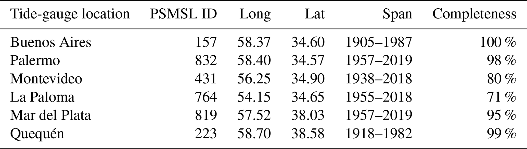
I use annual relative sea-level records from the Permanent Service for Mean Sea Level (PSMSL; Holgate et al., 2013; PSMSL, 2022). The PSMSL database extracted on 21 March 2022 provides long (>50-year) time series reduced to a common datum for six tide gauges from three regions in and around the Río de la Plata: Buenos Aires and Palermo towards the head of the estuary in Argentina, Montevideo and La Paloma near the mouth of the estuary along the coast of Uruguay to the north, and Mar del Plata and Quequén outside the estuary along coastal Argentina to the south (Table 2; Figs. 1, 4). To extend record length and to reduce dimensionality and errors, I average adjacent pairs of tide-gauge records relative to their common period, creating longer virtual station records (Dangendorf et al., 2017; Frederikse et al., 2021; Jevrejeva et al., 2014) at Buenos Aires (1905–2019), Montevideo (1938–2018), and Mar del Plata (1918–2019). For each station, I interrogate the period of overlap between virtual station and stream-gauge data.
Table 2PSMSL tide-gauge records (Holgate et al., 2013; Figs. 1, 4). Long and Lat are degrees west longitude and south latitude, respectively. Completeness is the percentage of years during the span that feature data.
2.3 Late Holocene trends
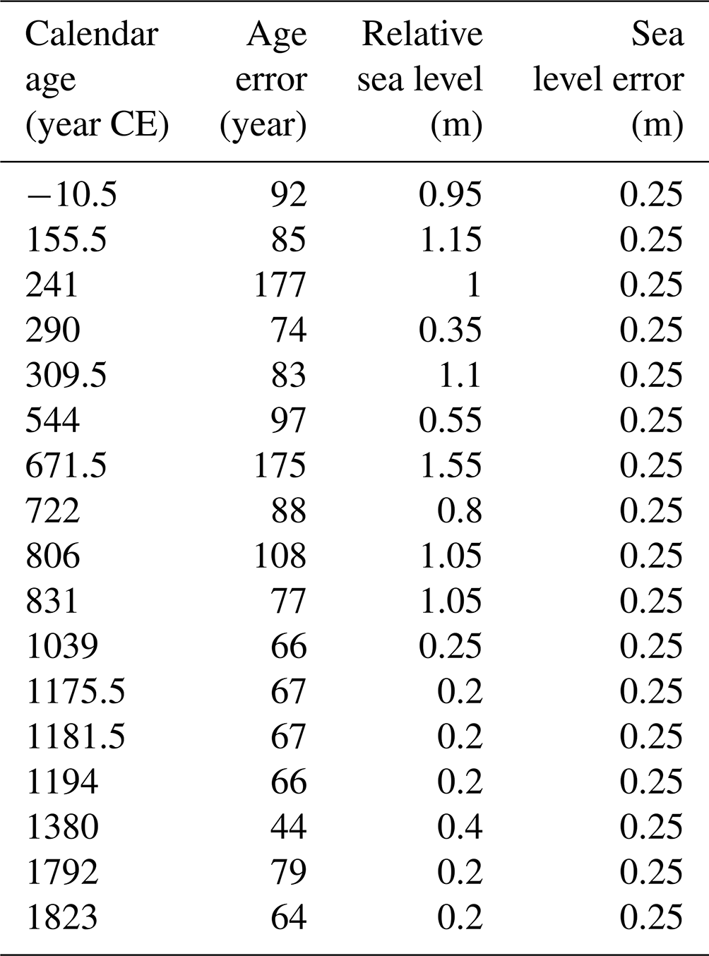
To distinguish late Holocene trends related to background geological processes from modern rates of change due to ocean circulation and climate in the tide-gauge records, I use proxy reconstructions of relative sea level from Santa Catarina, Brazil, compiled by Milne et al. (2005) and originally reported by Angulo et al. (1999) based on Vermetid snails (Table 3). These mollusks are sea-level indicators because they grow formations between the infra- and mid-littoral zones, so formations fossilized in growth position are informative of low water (Laborel, 1986). Applying Bayesian linear regression to the data and accounting for the relative sea level and age errors, I determine a relative sea-level trend during the past 2000 years of mm yr−1 (95 % posterior credible interval); the Bayesian model is detailed in Appendix A. This negative rate of change arises from ocean siphoning and continental levering (Mitrovica and Milne, 2002), and past modeling studies of the glacial isostatic adjustment process report similar rates over the past few millennia (Caron et al., 2018; Peltier, 2004).
Table 3Proxy sea-level reconstructions for the past 2 millennia from Santa Catarina (Milne et al., 2005). Milne et al. (2005) give calendar ages as min–max ranges, which I take to be 95 % confidence intervals. I take the center point as the best estimate and one-quarter of the range as 1 standard error. I also assume that sea-level errors given by Milne et al. (2005) correspond to 2 standard errors.
Mean Río de la Plata streamflow is m3 s−1 (Fig. 3), which is one of the largest river flows in the world, and consistent with values in past studies (Guerrero et al., 1997). Unless otherwise indicated, ± values identify 95 % bootstrap confidence intervals. The record standard deviation of m3 s−1 quantifies variability across interannual to multidecadal timescales, including a long-term trend of 96±37 m3 s−1 yr−1, which has been reported on previously (Dai, 2016; Dai et al., 2009). Interannual variations in streamflow partly correspond to the El Niño–Southern Oscillation (ENSO); the correlation coefficient between streamflow and the Niño 3.4 Index (Rayner et al., 2003) is 0.33±0.16, and peak streamflow occurred during the 1982–1983 and 1997–1998 El Niños. Such relationships between streamflow and ENSO have been extensively documented (Berri et al., 2002; Cardoso and Silva Dias, 2006; Depetris et al., 1996; Grimm et al., 1998; Robertson and Mechoso, 1998; Ropelewski and Halpert, 1987). Also apparent is a regime shift from the late 1960s to early 1980s when streamflow increased substantially. This transition has been ascribed to increased precipitation and decreased evaporation over the drainage basin due to changes in land use, deforestation, and large-scale climate modes (Lawrence and Vandecar, 2015; Medvigy et al., 2011).
The virtual station data similarly show that relative sea level varies over all periods (Fig. 4). These records also exhibit spatial structure. Detrended series at Buenos Aires and Montevideo are significantly correlated with one another (correlation coefficient 0.44±0.20), but neither is correlated with the detrended record at Mar del Plata (coefficients and 0.18±0.28, respectively). While the time series at Mar del Plata is uncorrelated with ENSO (correlation coefficient 0.12±0.17 with Niño 3.4), the records from Buenos Aires and Montevideo both show correlation with ENSO (coefficients 0.26±0.19 and 0.25±0.20 with Niño 3.4, respectively). These results are consistent with past studies (Douglas, 2001; Papadopoulous and Tsimplis, 2006; Raicich, 2008; Verocai et al., 2016) and suggest that there are processes that drive common sea-level changes at Buenos Aires and Montevideo but which do not affect sea level along Mar del Plata. Considering the longest timescales, I compute a long-term rate of change at Buenos Aires of 1.46±0.36 mm yr−1 based on ordinary least squares linear regression, which is larger than the trends of 1.03±0.53 and 1.00±0.35 mm yr−1 obtained for Montevideo and Mar del Plata, respectively (Fig. 7). These values agree with previous studies of regional sea-level rise cited in the Introduction. After adjusting for a late Holocene rate (Sect. 2.3; Fig. 5), I find an average sea-level trend across virtual stations of 1.70±0.40 mm yr−1, which is faster than modern estimates of twentieth-century global mean sea-level rise referenced earlier and similar to conclusions from Frederikse et al. (2021).
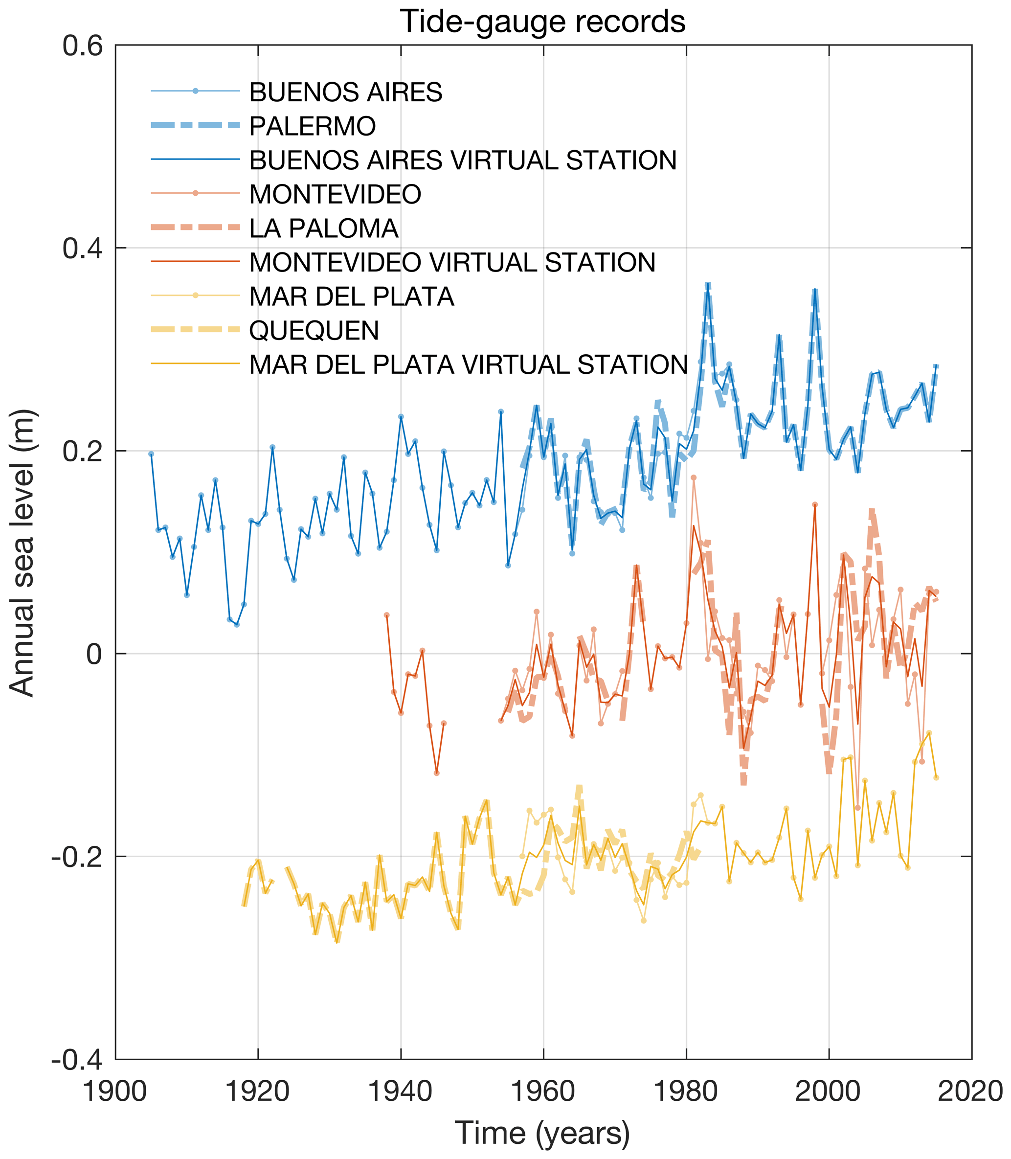
Figure 4Yearly tide-gauge relative sea-level records (Fig. 1, Table 2). Virtual station time series are shown as thick lines, and individual tide-gauge records are shown as thin lines. The time series are shifted vertically by an arbitrary amount for ease of visualization.
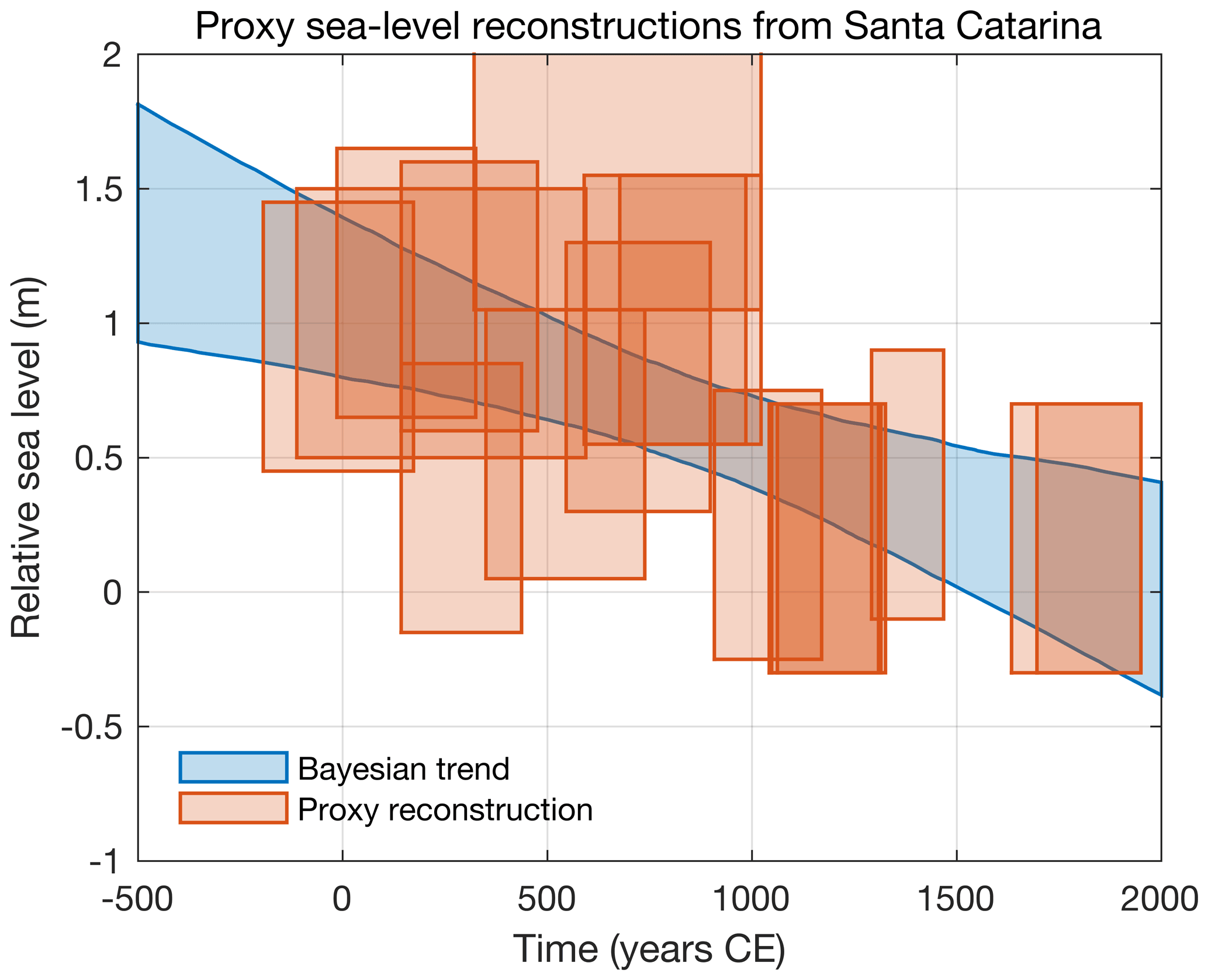
Figure 5Proxy sea-level reconstructions (orange) and Bayesian linear regression (blue). Orange shading identifies best estimates plus and minus twice the standard errors. Blue shading corresponds to 95 % posterior credible intervals. The Bayesian model is detailed in the Appendix.
Streamflow explains a substantial portion of the sea-level variation at Buenos Aires and to a lesser extent Montevideo, and it largely accounts for the apparent faster-than-global rate of regional sea-level rise (Figs. 6–8). To quantify the influence of streamflow on sea level, I evaluate a multiple linear regression model at each virtual station with sea level as the dependent variable and streamflow, time, and unity as the independent variables. The streamflow regressor explains 59±17 %, 28±21 %, and of the sea-level variance at Buenos Aires, Montevideo, and Mar del Plata, respectively (Fig. 6). This suggests that streamflow generally has more of an influence on sea level closer to the mouths of the Río Paraná and Río Uruguay. Regression coefficients between streamflow and sea level for Buenos Aires, Montevideo, and Mar del Plata are , , and m m−3 s, respectively (Fig. 7). This structure shows that sea level is more sensitive to streamflow closer to the mouths of the rivers. Finally, linear trends computed from the virtual station time series from this regression model are 0.75±0.34, 0.56±0.58, and 1.11±0.37 mm yr−1 at Buenos Aires, Montevideo, and Mar del Plata, respectively (Fig. 7). Compared to trends reported in the last paragraph, this implies that streamflow effected sea-level rates of 0.71±0.35, 0.48±0.38, and mm yr−1 at the respective virtual stations (Fig. 7). Averaging the streamflow-corrected sea-level trends and adjusting for the background geologic rate, I obtain a mean rate of 1.34±0.40 mm yr−1, which is more in line with recent global mean sea-level trends for the past century from Hay et al. (2015), Dangendorf et al. (2017), and Frederikse et al. (2020).
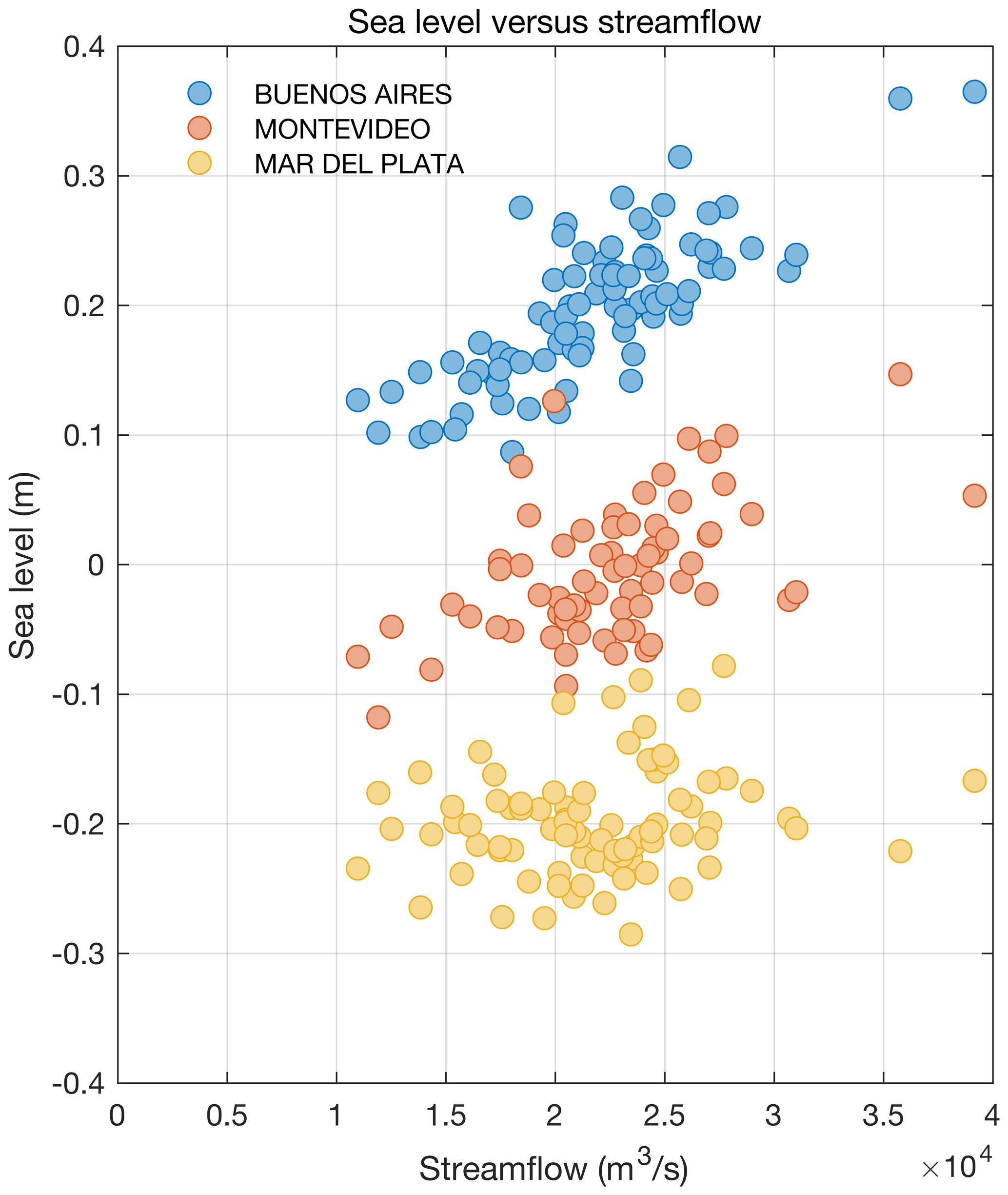
Figure 6Scatter plots comparing yearly average Río de la Plata streamflow (horizontal axes) and relative sea level (vertical axes) at Buenos Aires (blue), Montevideo (orange), and Mar del Plata (yellow). Sea-level values from the different sites are shifted vertically by an arbitrary amount for ease of visualization.
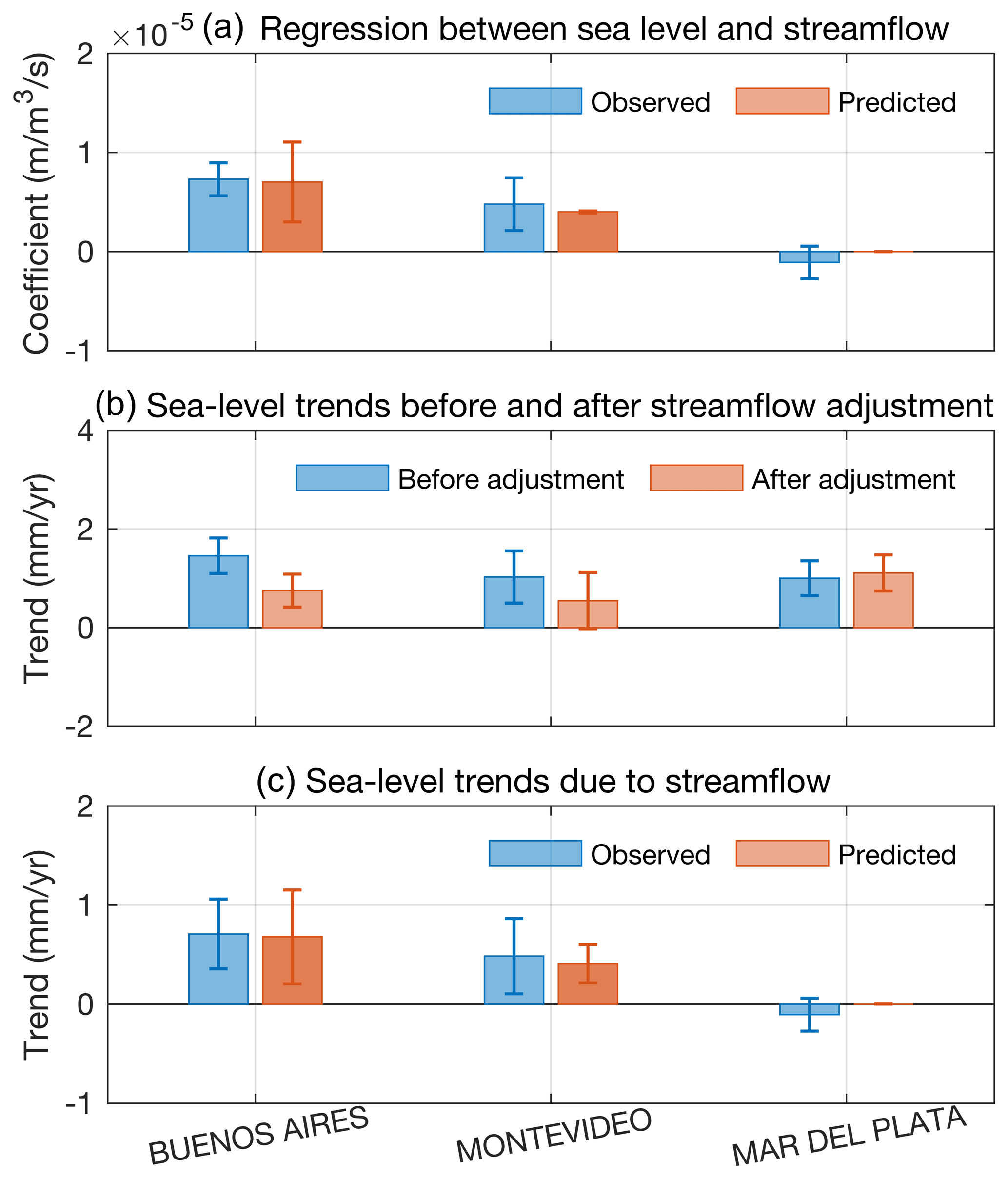
Figure 7(a) Regression coefficients between sea level and streamflow found empirically from linear regression (blue) and predicted theoretically from ocean dynamics (orange). (b) Trend computed from tide gauges without (blue) and with (orange) adjusting for river effects. (c) Sea-level trend due to streamflow found empirically from linear regression (blue) and predicted theoretically from ocean dynamics given the streamflow trend (orange). To evaluate predicted values at Buenos Aires, I use a value of x=65 km from the source in Eq. (13).
To establish the robustness of these results, I also consider alternative regression models and analysis approaches. First, I evaluate the same regression model but using ridge regression. This is meant to account for collinearity between predictors (e.g., the linear trend in streamflow). Results obtained for a wide range of ridge parameter values are essentially identical to the results found from ordinary least squares discussed earlier (not shown). From this, I conclude that the model is well posed and that collinearity between streamflow and time does not present a serious issue. Second, I evaluate the same regression model using ordinary least squares but considering sea-level and streamflow data with ENSO effects removed prior to analysis. I remove ENSO effects by regressing the quantity of interest against the Niño 3.4 Index and its Hilbert transform to capture arbitrary phase relationships between quantities. If river effects on sea level are restricted to ENSO events, then results from this analysis should give no meaningful relationship between sea level and streamflow. However, in this analysis, I find very similar regression coefficients between sea level and streamflow ( at Buenos Aires; at Montevideo; m m−3 s at Mar del Plata) as well as sea-level variance explained by streamflow (55±18 % at Buenos Aires; 21±19 % at Montevideo; at Mar del Plata) as previously when I did not remove ENSO effects prior to analysis. From this, I conclude that river effects on sea level in the Río de la Plata are not restricted to ENSO events, which have been the focus of past studies cited above, but are rather more general. This conclusion is consistent with results from wavelet coherence analysis (Grinsted et al., 2004). Streamflow is significantly coherent with sea level at Buenos Aires across most time periods and frequency bands resolved by the data, as well as with sea level at Montevideo for particular periods and frequencies (e.g., decadal scales generally, interannual scales during the 1990s and 2000s), but it is mostly incoherent with Mar del Plata sea level (Fig. 8).
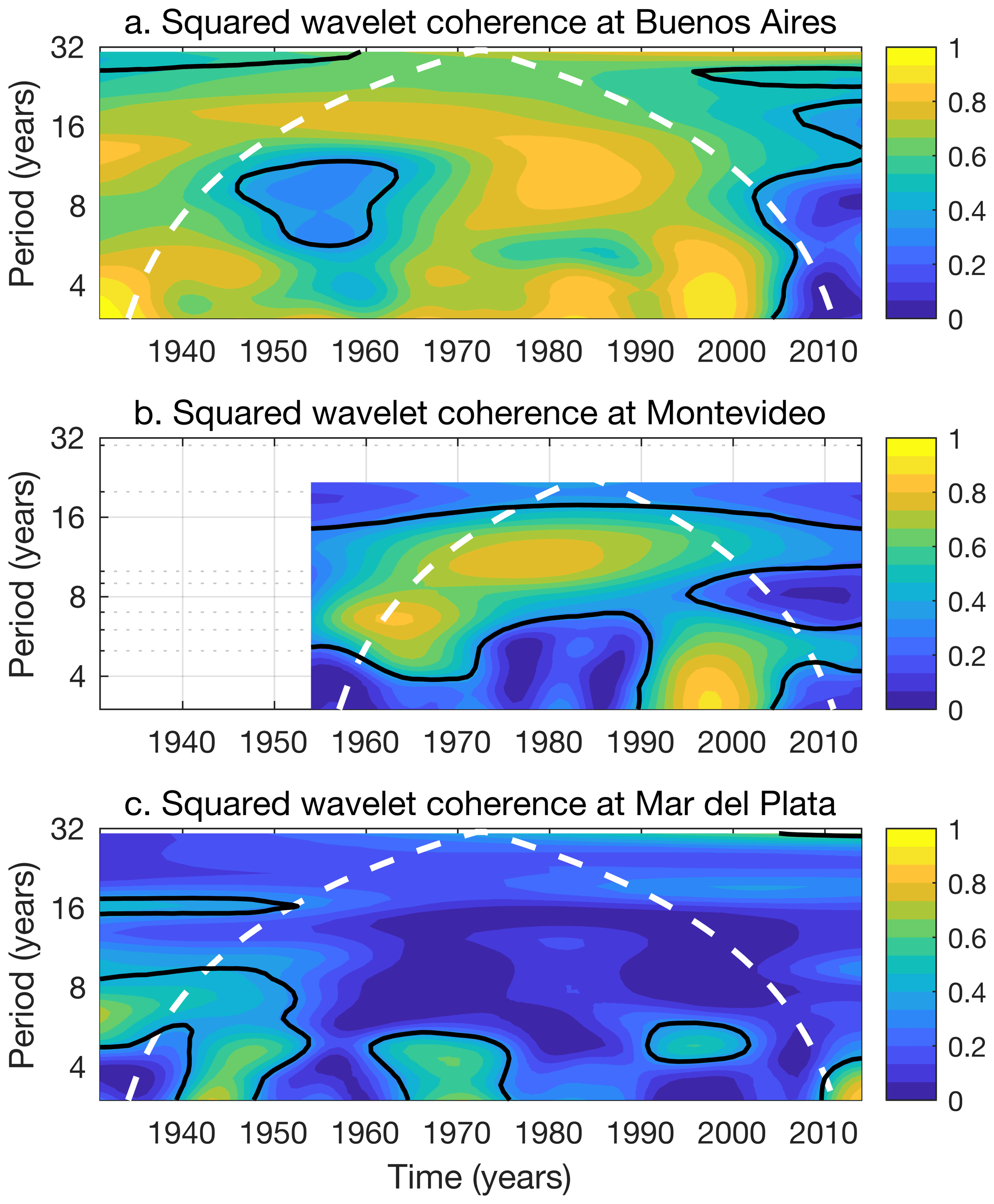
Figure 8Magnitude-squared wavelet coherence between streamflow and sea level at (a) Buenos Aires, (b) Montevideo, and (c) Mar del Plata. Solid black lines identify where values are significant at the 68 % confidence level, and white dashed lines mark the cone of influence. Statistical significance is determined from 1000 simulations with phase-scrambled versions of the observational data (Theiler et al., 1992). Values are based on the analytic Morlet wavelet.
Findings in the preceding section are based on correlation and regression analysis. They do not necessarily demonstrate that streamflow and coastal sea level are causally connected. To provide physical interpretation and establish causality, I develop simple theories for the relationship between streamflow and coastal sea level based on ocean dynamics in Sect. 4.1 and 4.2, and I compare model predictions to observational results in Sect. 4.3. To facilitate model development, I provide a schematic illustration of the region identifying key model quantities in Fig. 9.

Figure 9Schematic of the study region with key model quantities identified. The top shows a plan view of the region. The bottom shows cross sections at various locations in and around the Río de la Plata. Locations a and b are upstream near Buenos Aires, where the barotropic theory developed in Sect. 4.1 applies. Location c is downstream of Montevideo near La Paloma, where the baroclinic theory developed in Sect. 4.2 applies. At the bottom, yellow ⊗ identifies flow into the page, blue indicates fresher less dense water, and green denotes saltier more dense water. Other symbols and quantities are as defined in the text of Sect. 4.1 and 4.2. Illustration by Natalie Renier, WHOI.
4.1 Theory for Buenos Aires
Around Buenos Aires and Palermo, the Río de la Plata is relatively shallow, narrow, and fresh (Guerrero et al., 1997; Fig. 9). To model sea level in this region, I use the following conservation laws:
Here u, v, and w are velocities in along-estuary (x), across-estuary (y), and vertical (z) directions, respectively, p is hydrostatic pressure, ρf is a reference freshwater density, g is acceleration due to gravity, ν is kinematic viscosity, and x, y, and z subscripts are spatial derivatives (Fig. 9). Equations (1) and (2) are familiar forms of the continuity equation and hydrostatic balance (Gill, 1982). Equation (3) specifies along-estuary momentum conservation in terms of a balance between pressure gradient and viscous forces; it omits the time tendency given the long periods under consideration, and it also neglects nonlinear advection and Coriolis acceleration under the assumptions of a small Reynolds number and large Ekman number, which are reasonable given the spatial scales of the problem.
Integrating Eq. (1) over the depth H(x) and width W(x) of the estuary (Fig. 9), applying kinematic boundary conditions at the bottom and along the sides, and ignoring the time tendency gives
where the overbar and bracket are depth and across-estuary average, respectively. Integrating Eq. (2) vertically, substituting into Eq. (3), and averaging over depth and width yields
where ζ is ocean dynamic sea level, Cd is a drag coefficient, and U is a reference velocity scale. To obtain Eq. (5), I assumed that the ζ slope across the estuary is linear and that
along the bottom. To solve Eqs. (4) and (5) for 〈ζ〉, I specify that along-estuary transport equals the streamflow q at the origin,
and that 〈ζ〉 vanishes far from the source:
Combining Eqs. (4) and (7), substituting for in Eq. (5), integrating along the estuary from x to ∞, and applying the boundary condition from Eq. (8) gives
for arbitrary depth and width profiles. For an estuary with exponential width and depth (Fig. 2),
where W0 and H0 are initial values and LW and LH are length scales, the solution to Eq. (9) is
The 〈ζ〉 response is linear in q and controlled by friction and the geometry of the estuary; it is larger for stronger friction CdU, narrower initial width W0, shallower initial depth H0, longer width and depth scales LW and LH, and decays rapidly with distance from the origin (Fig. 10).
Regression coefficients computed between sea-level and streamflow data (Fig. 7) can be understood as approximate observational estimates of the derivative of the former with respect to the latter. From Eq. (12), it follows that
Below, I numerically evaluate Eq. (13) and compare the values to the empirically determined regression coefficients to test whether the theory is consistent with the observations.
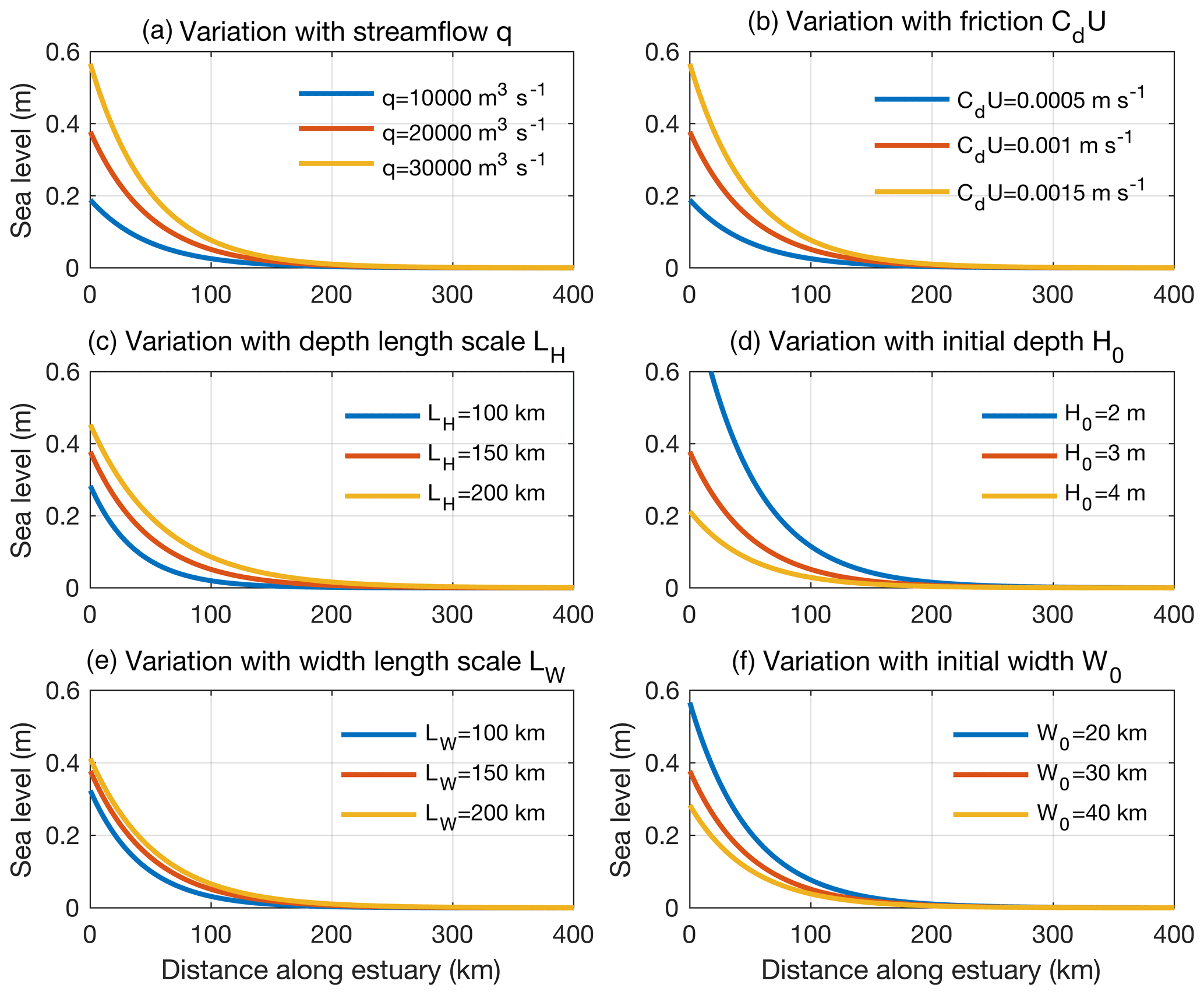
Figure 10Sea-level response 〈ζ〉 to streamflow forcing q described by Eq. (12) as a function of distance along the estuary away from the mouth of the rivers for different values of (a) streamflow q, (b) friction CdU, (c) depth length scale LH, (d) initial depth H0, (e) width length scale LW, and (f) initial width W0. Default values are m3 s−1, CdU=0.001 m s−1, LH=150 km, H0=2 m, LW=150 km, and W0=30 km.
4.2 Theory for Montevideo
The solution for Buenos Aires (Eq. 12) is not applicable to Montevideo. The estuary becomes wider, deeper, and more saline by this point (Guerrero et al., 1997; Figs. 1, 2, 9), so stratification and rotation effects cannot be neglected as they were previously. I develop a theory for the ζ response at Montevideo based on past studies of bottom-advected (slope-controlled) plumes (Chapman and Lentz, 1994; Lentz and Helfrich, 2002; Yankovsky and Chapman, 1997). I take x, y, and z to be the alongshore, across-shore, and vertical coordinates, respectively. As a mental model, I envision a narrow alongshore jet over a sloping bottom H(y) in thermal wind balance with a sharp density front at a location yp offshore (Fig. 9). I imagine the jet transport includes both the fresh river water and salty ocean water brought into the plume by turbulent mixing. These features are represented by the following governing equations:
where f=2Ωsin ϕ is the Coriolis frequency for Earth rotation rate Ω and latitude ϕ, ρ0 is an ambient ocean density, Q is volume transport of the vertically sheared geostrophic jet, and E is entrainment flux. Equations (14) and (15) are geostrophic and hydrostatic balances, respectively. Equation (16) is a form of the continuity equation, which states that volume is conserved within the jet. Density conservation in Eq. (17) is equivalent to steady-state heat and salt conservation for a linear equation of state1. Boundary conditions are that alongshore velocity vanishes everywhere along the bottom and that velocity shear is zero at the foot of the front (Chapman and Lentz, 1994; Lentz and Helfrich, 2002; Yankovsky and Chapman, 1997)
A solution to Eqs. (14)–(19) is obtained by giving a functional form to the density field. I picture an infinitely narrow front, with ambient ocean density everywhere offshore, and a mixture of fresh river water and salty ocean water onshore of the front, which I model as (Fig. 11a, b)
where ρ′ is a density increment and ℋ is the Heaviside step function. The alongshore velocity field in thermal wind balance with this density structure, obtained by cross-differentiating Eqs. (14) and (15) and then integrating vertically subject to the boundary conditions, is
where δ is the Dirac delta (Fig. 11c).

Figure 11Idealized (a) density structure onshore of the front (Eq. 20), (b) density structure offshore of the front (Eq. 21), and (c) velocity structure within the front (Eq. 21) as a function of depth. Sea-level response ζ described by Eq. (28) as a function of (d) streamflow q, (e) latitude ϕ, and (f) ambient ocean density ρ0. Default values: m3 s−1, , ρ0=1030 kg m−3.
To obtain the sea-level solution corresponding to Eq. (21), I integrate geostrophic balance at the surface,
over all offshore locations, which gives
That is, ζ takes on a constant value of onshore of the front, experiences a step change at the front, and vanishes offshore of the front. The ζ solution can be written more explicitly in terms of streamflow q and river and ocean densities ρf and ρ0 as follows. First, I express Q in terms of q and density. Given Eq. (20), the vertically averaged density within the front is
which, substituting into Eq. (17) and combining with Eq. (16) to eliminate E, implies
which is analogous to a form of Knudsen's hydrographical theorem (Dyer, 1997). Second, I solve for Hp in terms of Q and density. Integrating both sides of Eq. (21) over all depths and offshore locations and rearranging gives
or, after rearranging and solving for Hp (and recalling that f<0 in the Southern Hemisphere),
Finally, I substitute Eq. (25) for Q in Eq. (27), insert the resulting expression for Hp in Eq. (23), and cancel common terms to give
The ζ response is nonlinear in q and controlled by stratification and rotation; it is larger for higher latitude, stronger streamflow, and a sharper density contrast (Fig. 11d–f). While there is no alongshore dependence in Eq. (28), it assumes that the location of interest is downstream in the far field of the river mouth. Given Eq. (28), the derivative of ζ with respect to q, which can be evaluated numerically and compared to regression coefficients from observations, is
4.3 Model–data comparison
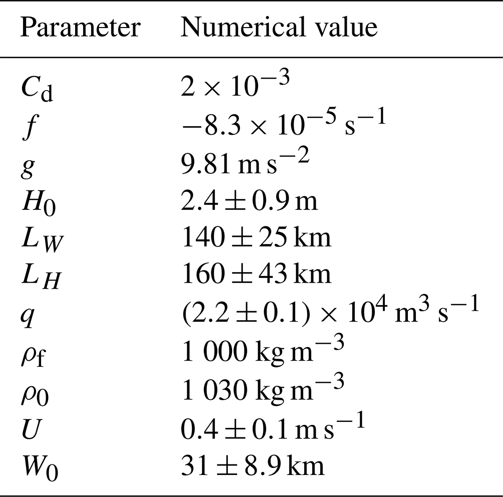
To test whether empirical results from Sect. 3 are consistent with theories developed in Sect. 4.1 and 4.2, I evaluate Eq. (13) for Buenos Aires and Eq. (29) for Montevideo using parameter values in Table 4 and then compare the predictions to the observed values (Fig. 7). See Appendix B for a discussion of the numerical values of the model parameters in Table 4. Equation (13) gives a theoretical regression coefficient between streamflow and sea level for Buenos Aires of m m−3 s, where the error bar reflects uncertainties in the parameter values (Table 4). Multiplying this coefficient by the long-term trend in streamflow estimated earlier (96±37 m3 s−1 yr−1), I obtain an expected sea-level trend at Buenos Aires due to streamflow of 0.68±0.47 mm yr−1. These theoretical estimates agree with the coefficient of m m−3 s and the streamflow-driven sea-level trend of 0.71±0.35 mm yr−1 found earlier from regression analysis of observed streamflow and sea level at Buenos Aires (Fig. 7). Following the same approach and evaluating Eq. (29), I find a theoretical regression coefficient of m m−3 s and an anticipated sea-level trend forced by streamflow of 0.41±0.19 mm yr−1 for Montevideo. Again, these values from first principles are consistent with the regression coefficient of m m−3 s and the streamflow-induced sea-level trend of 0.48±0.38 mm yr−1 found from the observational data (Fig. 7). The consistency between theory and observation suggests that the statistical connections found earlier between measured streamflow and sea level at Buenos Aires and Montevideo identify cause-and-effect relationships, which are consistent with the physics prescribed above.
Table 4Parameter values used to evaluate Eqs. (13) and (29). See Appendix B for a detailed discussion on how the numerical values of the model parameters were selected.
The lack of a significant relation between streamflow and sea level in Mar del Plata in the data (Figs. 6–8) is also consistent with the theories developed in Sect. 4.1 and 4.2. The response described by Eq. (12) imagines a rapid decay away from the rivers. Indeed, given its strong exponential dependence, the sea-level response predicted by this theory is vanishingly small at Mar del Plata (Figs. 1, 10). The response described by Eq. (28) envisions coastal sea level coupled to a buoyant longshore current in the sense of coastal waves: counterclockwise along the Uruguay coast and then equatorward along the Brazil coast (Piola et al., 2005). In other words, given this mechanism, Mar del Plata is not downstream of the Río de la Plata, and hence no signals are communicated between the two locations according to these physics.
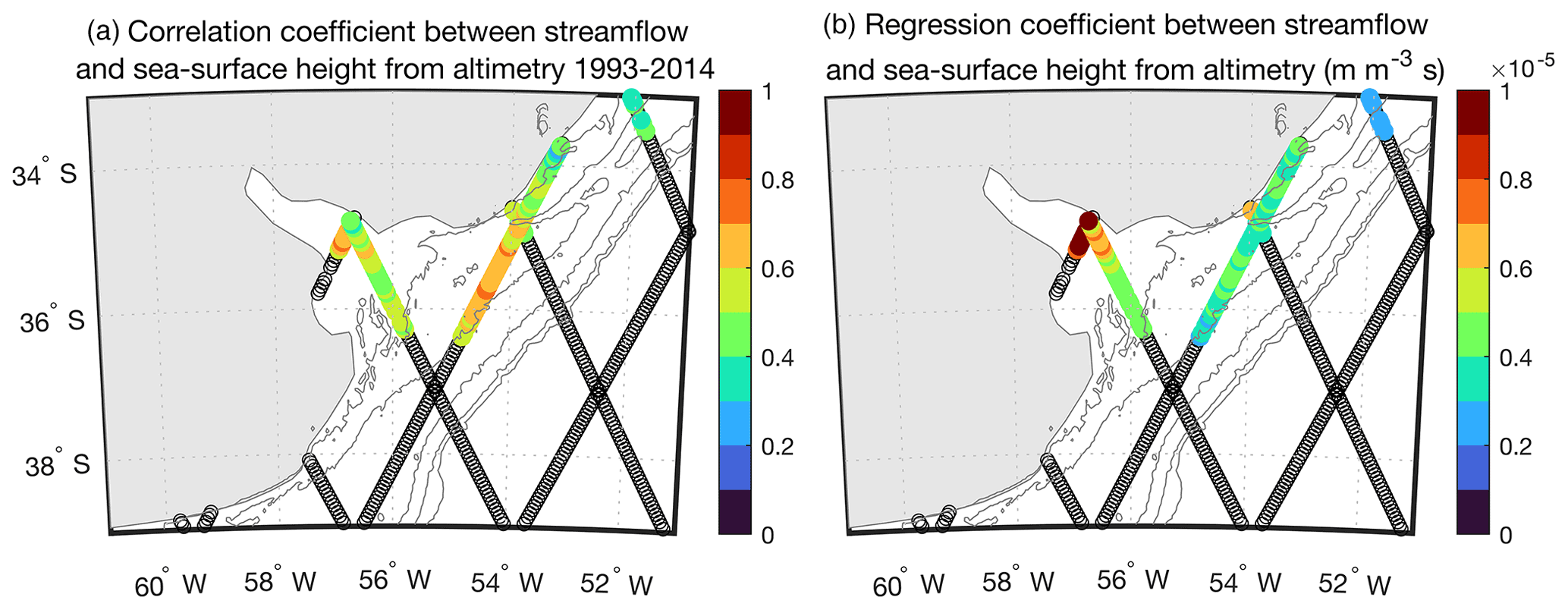
Figure 12(a) Correlation coefficient and (b) regression coefficient (m m−3 s) between annual streamflow in the Río de la Plata (Fig. 3) and sea surface height anomaly from along-track satellite altimetry data (Birol et al., 2017) during 1993–2014 over the study regions. Values are only shown where correlation coefficients are positive at the 95 % confidence level determined through bootstrapping. Contours identify the 20, 50, 100, 200, and 500 m isobaths.
The Río de la Plata estuary in South America features the longest tide-gauge records in the South Atlantic Ocean (Figs. 1, 2). However, the causes of long-term relative sea-level changes in this region have not been firmly established. I interrogated data (Figs. 3–5) and developed theories (Figs. 8–11) to argue for cause-and-effect relationships between low-frequency streamflow and sea-level changes in the Río de la Plata over 1931–2014 (Figs. 6, 7). Streamflow forcing generally explained one-half of the sea-level variance on interannual and longer timescales observed at Buenos Aires and one-quarter of the sea-level variance at Montevideo over the study period. Specifically, a trend in streamflow of ∼100 m3 s−1 yr−1 during the past century caused sea level to rise at rates of ∼0.7 mm yr−1 at Buenos Aires and ∼0.5 mm yr−1 at Montevideo. These findings advance understanding of local, regional, and global sea-level changes; clarify basic sea-level physics; inform future projections of coastal sea-level change as well as the interpretation of satellite data and proxy reconstructions; and highlight future research directions.
This paper complements past tide-gauge studies on mean sea-level changes in the Río de la Plata on interannual to centennial timescales (e.g., Aubrey et al., 1988; Brandani et al., 1985; D'Onofrio et al., 2008; Dennis et al., 1995; Douglas, 1997, 2001, 2008; Emery and Aubrey, 1991; Fiore et al., 2009; Frederikse et al., 2021; Isla, 2008; Lanfredi et al., 1998; Meccia et al., 2009; Melini et al., 2004; Papadopoulous and Tsimplis, 2006; Pousa et al., 2007; Raicich, 2008; Santamaria-Aguilar et al., 2017; Thompson et al., 2016; Verocai et al., 2016). Previous authors have established that streamflow and sea level in the Río de la Plata covary on interannual timescales during ENSO events, but they do not identify the causal mechanisms responsible for the observed statistical correlations, nor do they consider how these two variables correspond more generally on longer timescales. My paper builds on their foundation by showing that river effects on sea level are not restricted to ENSO events in particular, but are also apparent more generally at multidecadal and centennial periods, and by identifying ocean dynamic mechanisms that mediate the relationship between streamflow and sea level. These results corroborate the hypothesis due to Douglas (2001) that interannual sea-level variation at Buenos Aires over the 1982–1983 El Niño can be understood in terms of ocean dynamic processes, but they do not necessarily falsify suggestions that contemporary gravitational, rotational, and deformational effects also played a role (Isla, 2008; Thompson et al., 2016). Likewise, while they suggest that streamflow changes contributed importantly to long-term sea-level rise observed at Buenos Aires and Montevideo, these results do not rule out the possibility that other geophysical processes also effected regional sea-level trends (Melini et al., 2004; Aubrey et al., 1988).
My results have implications for twentieth-century global sea-level reconstructions and budgets (e.g., Church and White, 2011; Dangendorf et al., 2017; Frederikse et al., 2018, 2020, 2021; Hamlington and Thompson, 2015; Hay et al., 2015; Jevrejeva et al., 2014; Natarov et al., 2017; Ray and Douglas, 2011; Thompson and Merrifield, 2014; Thompson et al., 2016). The streamflow-driven sea-level effects highlighted here are local to regional in scale; they do not contribute meaningfully to sea-level changes on basin or global scales. Hence, such river effects on tide gauges in the Río de la Plata should be removed prior to analysis if the data are used in large-scale circulation and climate studies, lest this local or regional “noise” alias onto the basin or global “signal” of interest (e.g., Papadopoulous and Tsimplis, 2006; Thompson et al., 2016). Given the heavy weight placed on tide gauges from the Río de la Plata, streamflow-driven ocean dynamics could contribute to the lack of sea-level-budget closure and faster-than-global trends across the South Atlantic during the twentieth century found by Frederikse et al. (2018, 2021). Since tide-gauge records in and around the Río de la Plata are the main (if not sole) data constraint in the South Atlantic prior to 1950 in twentieth-century global mean sea-level reconstructions (Fig. 1b in Hamlington and Thompson, 2015; Fig. S1a in Dangendorf et al., 2017), it would be informative to estimate twentieth-century global mean sea-level rise from tide-gauge records adjusted for river effects, which are typically not considered in global budgets and reconstructions.
Theories developed here (Eqs. 13 and 29) clarify relationships between streamflow and coastal sea level, the physics of which have not been well understood (Durand et al., 2019). Piecuch et al. (2018a) formulate a theory for the far-field coastal sea-level response to buoyant river discharge in the limit of a pure surface-advected plume (their Eqs. 5 and 6). This study improves upon their work in two ways. First, I developed a barotropic theory for the sea-level response within an estuary (Eq. 13), where frictional effects and the shape of coastlines and bathymetry are important. Second, I formulated a far-field theory for the coastal sea-level adjustment in the alternative limit of a purely bottom-advected (or slope-controlled) plume (Eq. 29), which is more germane to the problem at hand. These new theories allow the relationship between sea level and river discharge to be studied in a wider range of settings. In a future study, I plan to develop a more general far-field theory for the buoyancy-driven sea-level response to an intermediate buoyant plume that falls between the extremes of a surface-advected plume and a bottom-advected plume (Yankovsky and Chapman, 1997; Lentz and Helfrich, 2002).
I demonstrated that the sea-level response to buoyant coastal discharge can depend sensitively on density gradients over short scales and the geometry of coastlines and bathymetry. With some exceptions (Haarsma et al., 2016), the current generation of coupled models used for climate projections is too coarsely resolved to represent such features (Holt et al., 2017). Theories developed here may be helpful in this regard. Equations (13) and (29) may be instructive for obtaining basic scales and magnitudes of future coastal sea-level changes due to streamflow, assuming that the details of coastlines and bathymetry are known and given projected changes in continental freshwater runoff into the coastal ocean. In the future, as global climate models with improved representation of the coastal ocean and shelf seas become more widely available, numerical experiments could be performed to broadly test analytical predictions made here regarding relationships between sea level and streamflow.
Due to my focus on long-term trends, I interrogated sea-level records from tide gauges. However, streamflow-driven sea-level changes are also apparent in data from other observing systems, including satellite altimetry. Comparing annual streamflow and sea surface height anomaly from along-track altimetry over 1993–2014 (Birol et al., 2017), I observe a region of significant correlation between the two variables extending broadly over the Uruguay coast from Montevideo past La Paloma towards Brazil and onshore of the ∼100 m isobath (Fig. 12a; see Fig. 1). The shape of the region mirrors the structure of low-salinity water near the mouth of the estuary (e.g., Piola et al., 2005). Regression coefficients obtained between Río de la Plata streamflow and sea surface height anomaly are consistent with theoretical expectations: more upstream in the estuary, values are m m−3 s, similar to predictions from barotropic theory developed in Sect. 4.1 (Eq. 13), whereas values downstream in the far field are m m−3 s, consistent with values anticipated from the baroclinic theory from Sect. 4.2 (Eq. 29) (Fig. 12b; see Fig. 7). The offshore extent of the region of significant correlation between streamflow and sea surface height also corroborates basic theoretical expectations: for strong slope control and large river discharge, the offshore and vertical scales of a buoyant coastal plume are expected to be ∼100 km and ∼100 m, respectively (e.g., Yankovsky and Chapman, 1997).
Findings here may have implications for proxy reconstructions of late Holocene sea level from natural archives, which have temporal resolution of decades to centuries (e.g., Kemp et al., 2009; Khan et al., 2019). Whereas past studies reason that river effects contribute to sea-level variability on interannual and shorter timescales (e.g., Durand et al., 2019; Woodworth et al., 2019), I showed that streamflow changes can be an important driver of sea-level changes over multidecadal and longer periods. This result has (at least) two important implications for proxy reconstructions. First, it implies that river effects may be important to consider when interpreting proxy sea-level reconstructions from large rivers or estuaries (e.g., Gerlach et al., 2017; Kemp et al., 2018). Second, it suggests that proxy sea-level reconstructions produced from strategic locations may inform past changes in streamflow and thus complement estimates from more traditional archives like tree rings (e.g., Margolis et al., 2011; Devineni et al., 2013).
Other major rivers including the Mississippi, Yenisey, and Lena have also undergone significant streamflow trends in the past century (e.g., Dai, 2016; Dai and Trenberth, 2002; Dai et al., 2009). However, the effect of these historical changes in streamflow on long-term sea-level change has not been considered. Future studies should take advantage of the growing number of available runoff and streamflow datasets (e.g., Do et al., 2018; Gudmundsson et al., 2018a; Tsujino et al., 2018) to test the analytical models developed here and observationally constrain river effects on historical sea-level rise more globally, which could inform studies of ocean circulation and climate change.
I apply Bayesian linear regression to proxy reconstructions from Milne et al. (2005) to quantify late Holocene rates of sea-level change. Bayesian linear regression is chosen over more traditional approaches like least squares or maximum likelihood because Bayesian methods provide a more transparent means for incorporating data errors into the formal uncertainty quantification. I design the Bayesian hierarchical model following similar algorithms developed in past studies (Ashe et al., 2019; Cahill et al., 2015, 2016; Walker et al., 2020). The model used here is essentially the time component of the space–time model from Piecuch et al. (2018b). While I give a brief description for the sake of completeness, readers are referred to Piecuch et al. (2018b) for a more detailed presentation.
Temporal Bayesian hierarchical models comprise three levels: a process level that prescribes the temporal evolution of the sea-level process, a data level that codifies the relationship between the uncertain proxy reconstructions and the sea-level process, and a parameter level at which prior constraints are specified.
For the process level, I model sea level as a linear function of time according to
where ∼ means “is distributed as”, 𝒩(a,b2) is the normal distribution with mean a and variance b2, and α, β, and γ2 are uncertain slope, intercept, and residual variance parameters, respectively. For the data level, I represent the proxy reconstructions of relative sea level and age as noisy versions of the respective processes, viz.,
where and are the data error variances, which are provided (Table 3). To close the model, I assume normal priors for α and β and an inverse-gamma prior for γ2,
where tildes identify fixed hyperparameters (see below for numerical values).
Given Bayes' rule and the model equations, I assume the posterior distribution is
where p is probability, | is conditionality, and ∝ indicates “proportional to”. To evaluate the posterior, I use a Gibbs sampler (Gelman et al., 2013), evaluating the full posteriors (Wikle and Berliner, 2007):
where is conditionality on all other processes, parameters, and data. I set weak, uninformative priors ( mm yr−1, mm2 yr−2, m, m2, , m2). I discard 1000 burn-in draws to eliminate startup transients. I reduce autocorrelation of the samples by keeping only every 10th draw of the subsequent 10 000 iterations of the Gibbs sampler. This gives a 1000-member ensemble of posterior estimates for y, x, α, β, and γ2. Figure 5 shows summary statistics for the posterior solution of αx+β for x from 500 BCE to present.
To evaluate Eqs. (13) and (29), numerical values need to be assigned to the various model parameters. Here I detail the rationale behind the values tabulated in Table 4.
I chose standard reference values for freshwater density ρf, seawater density ρ0, gravitational acceleration g, and the Coriolis parameter at the latitude of the Río de la Plata.
Ranges on the initial estuary width W0 and depth H0 as well as the width and depth scales LW and LH from Table 4 correspond to best estimates plus and minus 2 standard errors on these parameter values as determined by fitting exponentials in the form of Eqs. (10) and (11) to the bathymetry data in Fig. 2 using nonlinear least squares as described in the Fig. 2 caption.
The q value is the time mean of the Río de la Plata streamflow time series in Fig. 3 plus and minus twice its standard error.
Typical values for Cd range from 0.001 to 0.003 (Adcroft et al., 2018, 2019). I selected a middle-of-the-road value of 0.002.
The velocity scale U parameterizes the influence of unresolved processes and is typically selected to represent tidal motions (Adcroft et al., 2019). Regional tidal current amplitudes are 0.5–0.8 m s−1 (O'Connor, 1991; Piedra-Cueva and Fossati, 2007). Multiplying by a factor of , the average amplitude of a sine wave, gives the range of 0.3–0.5 m s−1 used here. This is larger than the background mean flow from river discharge, , which is 0.12 m s−1 at Buenos Aires (x=65 km), using the q, H0, W0, LH, and LW values in Table 4 discussed earlier.
All data used here are publicly available. Tide-gauge data are available through the Permanent Service for Mean Sea Level (https://www.psmsl.org/, Holgate et al., 2013). Stream-gauge data are available through the Global Streamflow Indices and Metadata Archive (https://doi.org/10.1594/PANGAEA.887470, Gudmundsson et al., 2018b). Proxy reconstructions are taken from the Appendix of Milne et al. (2005). Bathymetry data are available through the GEBCO Compilation Group (2021). Altimetry data are from the Center for Topographic studies of the Ocean and Hydrosphere (http://ctoh.legos.obs-mip.fr/, Birol et al., 2017). Wavelet coherence analysis was performed using code made available by Grinsted et al. (2004) (http://grinsted.github.io/wavelet-coherence/).
CGP was responsible for all aspects of this study including conceptualization, formal analysis, funding acquisition, investigation, methodology, visualization, and writing.
The author has declared that there are no competing interests.
Publisher's note: Copernicus Publications remains neutral with regard to jurisdictional claims in published maps and institutional affiliations.
Critical reviews by Francisco M. Calafat, Marcello Passaro, and two anonymous reviewers improved the paper. Helpful conversations with Roger C. Creel, Chris W. Hughes, Svetlana Jevrejeva, Caroline Katsman, Andrew C. Kemp, Steven J. Lentz, Kelly McKeon, Julius Oelsmann, Kristin Richter, and Anthony Wise are also acknowledged. This paper is a contribution by the International Space Science Institute (ISSI) Team on “Understanding the Connection Between Coastal Sea Level and Open Ocean Variability Through Space Observations” led by Francisco M. Calafat and Svetlana Jevrejeva.
This research has been supported by the National Aeronautics and Space Administration (grant nos. 80NSSC20K1241 and 80NM0018D0004) and the National Science Foundation (grant no. OCE-2002485).
This paper was edited by Joanne Williams and reviewed by two anonymous referees.
Acha, E. M., Mianzan, H., Guerrero, R., Carreto, J., Giberto, D., Montoya, N., and Carignan, M.: An overview of physical and ecological processes in the Rio de la Plata Estuary, Cont. Shelf Res., 28, 1579–1588, https://doi.org/10.1016/j.csr.2007.01.031, 2018.
Adcroft, A., Campin, J.-M., Dutkiewicz, S., Constantinos, E., Ferreira, D., Forget, G., Fox-Kemper, B., Heimbach, P., Hill, C., Hill, E., Hill, H., Jahn, O., Losch, M., Marshall, J., Maze, G., Menemenlis, D., and Molod, A.: MITgcm user manual, 485 pp., http://hdl.handle.net/1721.1/117188 (last access: 16 January 2023), 2018.
Adcroft, A., Anderson, W., Balaji, V., Blanton, C., Bushuk, M., Dufour, C. O., Dunne, J. P., Griffies, S. M., Hallberg, R., Harrison, M. J., Held, I. M., Jansen, M. F., John, J. G., Krasting, J. P., Langenhorst, A. R., Legg, S., Liang, Z., McHugh, C., Radhakrishnan, A., Reichl, B. G., Rosati, T., Samuels, B. L., Shao, A., Stouffer, R., Winton, M., Wittenberg, A. T., Xiang, B., and Zhang, R.: The GFDL global ocean and sea ice model OM4.0: Model description and simulation features, J. Adv. Model. Earth Syst., 11, 3167–3211, https://doi.org/10.1029/2019MS001726, 2019.
Angulo, R. J., Giannini, P. C. F., Suguio, K., and Pessendam, L. C. R.: Relative sea-level changes in the last 5500 years in southern Brazil (Laguna-Imbituba region, Santa Catarina State) based on vermetid 14C ages, Mar. Geol., 159, 323–339, https://doi.org/10.1016/S0025-3227(98)00204-7, 1999.
Ashe, E. L., Cahill, N., Hay, C., Khan, N. S., Kemp, A., Engelhart, S. E., Horton, B. P., Parnell, A. C., and Kopp, R. E.: Statistical modeling of rates and trends in Holocene relative sea level, Quaternary Sci. Rev., 204, 58–77, https://doi.org/10.1016/j.quascirev.2018.10.032, 2019.
Aubrey, D. G., Emery, K. O., and Uchupi, E.: Changing coastal levels of South America and the Caribbean region from tide-gauge records, Tectonophysics, 154, 269–284, https://doi.org/10.1016/0040-1951(88)90108-4, 1988.
Berri, G. J., Ghietto, M. A., and García, N. O.: The Influence of ENSO in the flows of the upper Paraná River of South America over the past 100 years, J. Hydrometeorol., 3, 57–65, https://doi.org/10.1175/1525-7541(2002)003<0057:TIOEIT>2.0.CO;2, 2002.
Birol, F., Fuller, N., Lyard, F., Cancet, M., Niño, F., Delebecque, C., Fleury, S., Toublanc, F., Melet, A., Saraceno, M., and Léger, F.: Coastal applications from nadir altimetry: Example of the X-TRACK regional products, Adv. Space Res., 59, 936–953, https://doi.org/10.1016/j.asr.2016.11.005, 2017 (data available at http://ctoh.legos.obs-mip.fr/, last access: 17 January 2023).
Brandani, A. A., D'Onofrio, E. E., and Schnack, E. J.: Comparative analysis of historical mean sea level changes along the Argentine coast, in: Quaternary of South America and Antarctic Peninsula, edited by: Rabassa, J., Balkema, Rotterdam, 187–195, ISBN: 9789061917847, 1985.
Cahill, N., Kemp, A. C., Horton, B. P., and Parnell, A. C.: Modeling sea-level change using errors-in-variables integrated Gaussian processes, Ann. Appl. Stat., 9, 547–571, https://doi.org/10.1214/15-AOAS824, 2015.
Cahill, N., Kemp, A. C., Horton, B. P., and Parnell, A. C.: A Bayesian hierarchical model for reconstructing relative sea level: from raw data to rates of change, Clim. Past, 12, 525–542, https://doi.org/10.5194/cp-12-525-2016, 2016.
Cardoso, A. O., and Silva Dias, P. L.: The relationship between ENSO and Paraná River flow, Adv. Geosci., 6, 189–193, https://doi.org/10.5194/adgeo-6-189-2006, 2006.
Caron, L., Ivins, E. R., Larour, E., Adhikari, S., Nilsson, J., and Blewitt, G.: GIA model statistics for GRACE hydrology, cryosphere, and ocean science, Geophys. Res. Lett., 45, 2203–2212, https://doi.org/10.1002/2017GL076644, 2018.
Chapman, D. C., and Lentz, S. J.: Trapping of a coastal density front by the bottom boundary layer, J. Phys. Oceanogr., 24, 1464–1479, https://doi.org/10.1175/1520-0485(1994)024<1464:TOACDF>2.0.CO;2, 1994.
Church, J. A., and White, N. J.: Sea-level rise from the late 19th to the early 21st century, Surv. Geophys., 32, 585–602, https://doi.org/10.1007/s10712-011-9119-1, 2011.
D'Onofrio, E. E., Fiore, M. M. E., and Pousa, J. L.: Changes in the regime of storm surges at Buenos Aires, Argentina, J. Coast. Res., 24, 260–265, https://doi.org/10.2112/05-0588.1, 2008.
Dai, A.: Historical and future changes in streamflow and continental runoff: a review, in: Terrestrial Water Cycle and Climate Change: Natural and Human-Induced Impacts, edited by: Tang, Q. and Oki, T., American Geophysical Union, Washington, DC, 17–37, ISBN: 978-1-118-97176-5, 2016.
Dai, A. and Trenberth, K. E.: Estimates of freshwater discharge from continents: latitudinal and seasonal variations, J. Hydrometeorol., 3, 660–687, https://doi.org/10.1175/1525-7541(2002)003<0660:EOFDFC>2.0.CO;2, 2002.
Dai, A., Qian, T., Trenberth, K. E., and Milliman, J. D.: Changes in continental freshwater discharge from 1948 to 2004, J. Clim., 22, 2773–2792, https://doi.org/10.1175/2008JCLI2592.1, 2009.
Dangendorf, S., Marcos, M., Wöppelmann, G., Conrad, C. P., Frederikse, T., and Riva, R.: Reassessment of 20th century global mean sea level rise, P. Natl. Acad. Sci. USA, 114, 5946–5951, https://doi.org/10.1073/pnas.1616007114, 2017.
Dennis, K. C., Schnack, E. J., Mouzo, F. H., and Orona, C. R.: Sea-level rise and Argentina: potential impacts and consequences, J. Coast. Res., 14, 205–223, https://www.jstor.org/stable/25735709 (last access: 16 January 2023), 1995.
Depetris, P. J., Kempe, S., Latif, M., and Mook, W. G.: ENSO-controlled flooding in the Paraná River (1904–1991), Naturwissenschaften, 83, 127–129, https://doi.org/10.1007/BF01142177, 1996.
Devineni, N., Lall, U., Pederson, N., and Cook, E.: A tree-ring-based reconstruction of Delaware River Basin streamflow using hierarchical Bayesian regression, J. Clim., 26, 4357–4374, https://doi.org/10.1175/JCLI-D-11-00675.1, 2013.
Do, H. X., Gudmundsson, L., Leonard, M., and Westra, S.: The global streamflow indices and metadata archive (GSIM) – Part 1: the production of a daily streamflow archive and metadata, Earth Syst. Sci. Data, 10, 765–785, https://doi.org/10.5194/essd-10-765-2018, 2018.
Douglas, B. C.: Global sea level rise: a redetermination, Surv. Geophys., 18, 279–292, https://doi.org/10.1023/A:1006544227856, 1997.
Douglas, B. C.: Sea level change in the era of the recording tide gauge, in: Sea Level Rise: History and Consequences, edited by: Douglas, B. C., Kearney, M. S., and Leatherman, S. P., International Geophysics Series, Vol. 75, Academic Press, San Diego, 37–64, ISBN-10: 012391146X, 2001.
Douglas, B. C.: Concerning evidence for fingerprints of glacial melting, J. Coast. Res., 24, 218–227, https://doi.org/10.2112/06-0748.1, 2008.
Durand, F., Piecuch, C. G., Becker, M., Papa, F., Raju, S. V., Khan, J. U., and Ponte, R. M.: Impact of coastal freshwater runoff on coastal sea level, Surv. Geophys., 40, 1437–1466, https://doi.org/10.1007/s10712-019-09536-w, 2019.
Dyer, K. R.: Estuaries: A Physical Introduction, Wiley, Chichester, 210 pp., ISBN: 978-0-471-97471-0, 1997.
Emery, K. O. and Aubrey, D. G.: Sea Levels, Land Levels, and Tide Gauges, Springer-Verlag, New York, 238 pp., ISBN-10: 1461391032, 1991.
Fiore, M. M. E., D'Onofrio, E. E., Pousa, J. L., Schnack, E. J., and Bértola, G. R.: Storm surges and coastal impacts at Mar del Plata, Argentina, Cont. Shelf Res., 29, 1643–1649, https://doi.org/10.1016/j.csr.2009.05.004, 2009.
Frederikse, T., Jevrejeva, S., Riva, R. E. M., and Dangendorf, S.: A consistent sea-level reconstruction and its budget on basin and global scales over 1958–2014, J. Clim., 31, 1267–1280, https://doi.org/10.1175/JCLI-D-17-0502.1, 2018.
Frederikse, T., Landerer, F., Caron, L., Adhikari, S., Parkes, D., Humphrey, V. W., Dangendorf, S., Hogarth, P., Zanna, L., Cheng, L., and Wu, Y.-H.: The causes of sea-level rise since 1900, Nature, 584, 393–397, https://doi.org/10.1038/s41586-020-2591-3, 2020.
Frederikse, T., Adhikari, S., Daley, T. J., Dangendorf, S., Gehrels, R., Landerer, F., Marcos, M., Newton, T. L., Rush, G., Slangen, A. B. A., and Wöppelmann, G.: Constraining 20th-century sea-level rise in the South Atlantic Ocean, J. Geophys. Res.-Ocean., 126, e2020JC016970, https://doi.org/10.1029/2020JC016970, 2021.
GEBCO Compilation Group: The GEBCO_2021 Grid – a continuous terrain model of the global oceans and land, NERC EDS British Oceanographic Data Centre NOC [data set], https://doi.org/10.5285/c6612cbe-50b3-0cff-e053-6c86abc09f8f, 2021.
Gelman, A., Carlin, J. B., Stern, H. S., Dunson, D. B., Vehtari, A., and Rubin, D. B.: Bayesian Data Analysis, Third Edition, Texts in Statistical Science, Chapman and Hall/CRC, Boca Raton, 675 pp., ISBN-10: 1439840954, 2013.
Gerlach, M. J., Engelhart, S. E., Kemp, A. C., Moyer, R. P., Smoak, J. M., Bernhardt, C. E., and Cahill, N.: Reconstructing Common Era relative sea-level change on the Gulf Coast of Florida, Mar. Geol., 390, 254–269, https://doi.org/10.1016/j.margeo.2017.07.001, 2017.
Gill, A. E.: Atmosphere-Ocean Dynamics. International Geophysics Series, Vol. 30, Academic Press, San Diego, 680 pp., ISBN-10: 0122835220, 1982.
Gregory, J. M., Griffies, S. M., Hughes, C. W., Lowe, J. A., Church, J. A., Fukumori, I., Gomez, N., Kopp, R. E., Landerer, F., Le Cozannet, G., Ponte, R. M., Stammer, D., Tamisiea, M. E., and van de Wal, R. S. W.: Concepts and terminology for sea level: mean, variability and change, both local and global, Surv. Geophys., 40, 1251–1289, https://doi.org/10.1007/s10712-019-09525-z, 2019.
Grimm, A. M., Ferraz, S. E. T., and Gomes, J.: Precipitation anomalies in southern Brazil associated with El Niño and La Niña events, J. Clim., 11, 2863–2880, https://doi.org/10.1175/1520-0442(1998)011<2863:PAISBA>2.0.CO;2, 1998.
Grinsted, A., Moore, J. C., and Jevrejeva, S.: Application of the cross wavelet transform and wavelet coherence to geophysical time series, Nonlinear Proc. Geoph., 11, 561–566, https://doi.org/10.5194/npg-11-561-2004, 2004 (data available at http://grinsted.github.io/wavelet-coherence/, last access: 17 January 2023).
Gudmundsson, L., Do, H. X., Leonard, M., and Westra, S.: The global streamflow indices and metadata archive (GSIM) – Part 2: quality control, tim-series indices and homogeneity assessment, Earth Syst. Sci. Data, 10, 787–804, https://doi.org/10.5194/essd-10-787-2018, 2018a.
Gudmundsson, L., Do, H. X., Leonard, M., and Westra, S.: The Global Streamflow Indices and Metadata Archive (GSIM) – Part 2: Time Series Indices and Homogeneity Assessment, PANGAEA [data set], https://doi.org/10.1594/PANGAEA.887470, 2018b.
Guerrero, R. A., Acha, E. M., Framiñan, M. B., and Lasta, C. A.: Physical oceanography of the Rió de la Plata estuary, Argentina, Cont. Shelf Res., 17, 727–742, https://doi.org/10.1016/S0278-4343(96)00061-1, 1997.
Haarsma, R. J., Roberts, M. J., Vidale, P. L., Senior, C. A., Bellucci, A., Bao, Q., Chang, P., Corti, S., Fuckar, N. S., Guemas, V., von Hardenberg, J., Hazeleger, W., Kodama, C., Koenigk, T., Leung, L. R., Lu, J., Luo, J.-J., Mao, J., Mizielinski, M. S., Mizuta, R., Nobre, P., Satoh, M., Scoccimarro, E., Semmler, T., Small, J., and von Storch, J.-S.: High Resolution Model Intercomparison Project (HighResMip v1.0) for CMIP6, Geosci. Model Dev., 9, 4185–4209, https://doi.org/10.5194/gmd-9-4185-2016, 2016.
Hamlington, B. D. and Thompson, P. R.: Considerations for estimating the 20th century trend in global mean sea level, Geophys. Res. Lett., 42, 4102–4109, https://doi.org/10.1002/2015GL064177, 2015.
Hay, C. C., Morrow, E., Kopp, R. E., and Mitrovica, J. X.: Probabilistic reanalysis of twentieth-century sea-level rise, Nature, 517, 481–484, https://doi.org/10.1038/nature14093, 2015.
Hogarth, P.: Preliminary analysis of acceleration of sea level rise through the twentieth century using extended tide gauge data sets (August 2014), J. Geophys. Res.-Ocean., 119, 7645–7659, https://doi.org/10.1002/2014JC009976, 2014.
Holgate, S. J., Matthews, A., Woodworth, P. L., Rickards, L. J., Tamisiea, M. E., Bradshaw, E., Foden, P. R., Gordon, K. M., Jevrejeva, S., and Pugh, J.: New data systems and products at the Permanent Service for Mean Sea Level, J. Coast. Res., 29, 493–504, https://doi.org/10.2112/JCOASTRES-D-12-00175.1, 2013 (data avaialable at: https://www.psmsl.org/, last access: 17 January 2023).
Holt, J., Hyder, P., Ashworth, M., Harle, J., Hewitt, H. T., Liu, H., New, A. L., Pickles, S., Porter, A., Popova, E., Allen, J. I., Siddorn, J., and Wood, R.: Prospects for improving the representation of coastal and shelf seas in global ocean models, Geosci. Model Dev., 10, 499–523, https://doi.org/10.5194/gmd-10-499-2017, 2017.
Horton, B. P., Kopp, R. E., Garner, A. J., Hay, C. C., Khan, N. S., Roy, K., and Shaw, T. A.: Mapping sea-level change in time, space, and probability, Annu. Rev. Env. Resour., 43, 481–521, https://doi.org/10.1146/annurev-environ-102017-025826, 2018.
Isla, F. I.: ENSO-dominated estuaries of Buenos Aires: the interannual transfer of water from western to eastern South America, Glob. Planet. Change, 64, 69–75, https://doi.org/10.1016/j.gloplacha.2008.09.002, 2008.
Jevrejeva, S., Moore, J. C., Grinsted, A., Matthews, A. P., and Spada, G.: Trends and acceleration in global and regional sea levels since 1807, Glob. Planet. Change, 113, 11–22, https://doi.org/10.1016/j.gloplacha.2013.12.004, 2014.
Kemp, A. C., Horton, B. P., Culver, S. J., Corbett, D. R., van de Plassche, O., Gehrels, W. R., Douglas, B. C., and Parnell, A. C.: Timing and magnitude of recent accelerated sea-level rise (North Carolina, United States), Geology, 37, 1035–1038, https://doi.org/10.1130/G30352A.1, 2009.
Kemp, A. C., Wright, A. J., Edwards, R. J., Barnett, R. L., Brain, M. J., Kopp, R. E., Cahill, N., Horton, B. P., Charman, D. J., Hawkes, A. D., Hill, T. D., and van de Plassche, O.: Relative sea-level change in Newfoundland, Canada during the past ∼3000 years, Quaternary Sci. Rev., 201, 89–110, https://doi.org/10.1016/j.quascirev.2018.10.012, 2018.
Khan, N. S., Horton, B. P., Engelhart, S., Rovere, A., Vacchi, M., Ashe, E. L., Törnqvist, T. E., Dutton, A., Hijma, M. P., Shennan, I., and the HOLSEA working group: Inception of a global atlas of sea levels since the Last Glacial Maximum, Quaternary Sci. Rev., 220, 359–371, https://doi.org/10.1016/j.quascirev.2019.07.016, 2019.
Kopp, R. E., Hay, C. C., Little, C. M., and Mitrovica, J. X.: Geographic variability of sea-level change, Curr. Clim. Change Rep., 1, 192–204, https://doi.org/10.1007/s40641-015-0015-5, 2015.
Laborel, J.: Vermetid gastropods as sea-level indicators, in: Sea-level research: a manual for the collection and evaluation of data, edited by: van de Plassche, O., Free University, Amsterdam, Netherlands, pp. 281–310, 1986.
Lanfredi, N. W., D'Onofrio, E. E., and Mazio, C. A.: Variations of the mean sea level in the southwest Atlantic Ocean, Cont. Shelf Res., 8, 1211–1220, https://doi.org/10.1016/0278-4343(88)90002-7, 1988.
Lanfredi, N. W., Pousa, J. L., and D'Onofrio, E. E.: Sea-level rise and related potential hazards on the Argentine coast, J. Coast. Res., 14, 47–60, https://www.jstor.org/stable/4298761 (last access: 16 January 2023), 1998.
Lawrence, D. and Vandecar, K.: Effects of tropical deforestation on climate and agriculture, Nat. Clim. Change, 5, 27–36, https://doi.org/10.1038/nclimate2430, 2015.
Lentz, S. J. and Helfrich, K. R.: Buoyant gravity currents along a sloping bottom in a rotating fluid, J. Fluid Mech., 464, 251–278, https://doi.org/10.1017/S0022112002008868, 2002.
Lisitzin, E.: Sea-Level Changes, Elsevier Oceanography Series, 8, Elsevier, Amsterdam, 286 pp., ISBN-10: 0444552871, 1974.
Margolis, E. Q., Meko, D. M., and Touchan, R.: A tree-ring reconstruction of streamflow in the Santa Fe River, New Mexico, J. Hydrol., 397, 118–127, https://doi.org/10.1016/j.jhydrol.2010.11.042, 2011.
Meccia, V. L., Simionato, C. G., Fiore, M. E., D'Onofrio, E. E., and Dragani, W. C.: Sea surface height variability in the Rio de la Plata estuary from synoptic to inter-annual scales: results of numerical simulations, Estuar. Coast. Shelf Sci., 85, 327–343, https://doi.org/10.1016/j.ecss.2009.08.024, 2009.
Medvigy, D., Walko, R. L., and Avissar, R.: Effects of deforestation on spatiotemporal distributions of precipitation in South America, J. Clim., 24, 2147–2163, https://doi.org/10.1175/2010JCLI3882.1, 2011.
Melini, D., Piersanti, A., Spada, G., Soldati, G., Casarotti, E., and Boschi, E.: Earthquakes and relative sealevel changes, Geophys. Res. Lett., 31, L09601, https://doi.org/10.1029/2003GL019347, 2004.
Milne, G. A., Long, A. J., and Bassett, S. E.: Modelling Holocene relative sea-level observatoins from the Caribbean and South America, Quaternary Sci. Rev., 24, 1183–1202, https://doi.org/10.1016/j.quascirev.2004.10.005, 2005.
Mitrovica, J. X. and Milne, G. A.: On the origin of late Holocene sea-level highstands within equatorial ocean basins, Quaternary Sci. Rev., 21, 2179–2190, https://doi.org/10.1016/S0277-3791(02)00080-X, 2002.
Moreira, D. and Simionato, C.: The Río de la Plata estuary hydrology and circulation, Meteorologica, 44, 1–30, 2019.
Natarov, S. I., Merrifield, M. A., Becker, J. M., and Thompson, P. R.: Regional influences on reconstructed global mean sea level, Geophys. Res. Lett., 44, 3274–3282, https://doi.org/10.1002/2016GL071523, 2017.
O'Connor, W. P.: A numerical model of tides and storm surges in the Rio de la Plata Estuary, Cont. Shelf Res., 11, 1491–1508, https://doi.org/10.1016/0278-4343(91)90023-Y, 1991.
Papadopoulous, A. and Tsimplis, M. N.: Coherent coastal sea-level variability at interdecadal and interannual scales from tide gauges, J. Coast. Res., 22, 625–639, https://doi.org/10.2112/04-0156.1, 2006.
Peltier, W. R.: Global glacial isostasy and the surface of the ice-age Earth: the ICE-5G (VM2) model and GRACE, Annu. Rev. Earth Pl. Sc., 32, 111–149, https://doi.org/10.1146/annurev.earth.32.082503.144359, 2004.
PSMSL (Permanent Service for Mean Sea Level): Tide gauge data, http://www.psmsl.org/data/obtaining/ (last access: 16 January 2023), 2022.
Piecuch, C. G., Bittermann, K., Kemp, A. C., Ponte, R. M., Little, C. M., Engelhart, S. E., and Lentz, S. J.: River-discharge effects on United States Atlantic and Gulf coast sea-level changes, P. Natl. Acad. Sci. USA, 115, 7729–7734, https://doi.org/10.1073/pnas.1805428115, 2018a.
Piecuch, C. G., Huybers, P., Hay, C. C., Kemp, A. C., Little, C. M., Mitrovica, J. X., Ponte, R. M., and Tingley, M. P.: Origin of spatial variation in US East Coast sea-level trends during 1900–2017, Nature, 564, 400–404, https://doi.org/10.1038/s41586-018-0787-6, 2018b.
Piedra-Cueva, I. and Fossati, M.: Residual currents and corridor of flow in the Rio de la Plata, Appl. Mathemat. Model., 31, 564–577, https://doi.org/10.1016/j.apm.2005.11.033, 2007.
Piola, A. R., Matano, R. P., Palma, E. D., Möller, O. O., and Campos, E. J. D.: The influence of the Plata River discharge on the western South Atlantic shelf, Geophys. Res. Lett., 32, L01603, https://doi.org/10.1029/2004GL021638, 2005.
Pousa, J., Tosi, L., Kruse, E., Guaraglia, D., Bonardi, M., Mazzoldi, A., Rizzetto, F., and Schnack, E.: Coastal processes and environmental hazards: the Buenos Aires (Argentina) and Venetian (Italy) littorals, Environ. Geol., 51, 1307–1316, https://doi.org/10.1007/s00254-006-0424-9, 2007.
Raicich, F.: A review of sea level observations and low frequency sea-level variability in the South Atlantic, Phys. Chem. Earth, 33, 239–249, https://doi.org/10.1016/j.pce.2007.04.001, 2008.
Ray, R. D. and Douglas, B. C.: Experiments in reconstructing twentieth-century sea levels, Prog. Oceanogr., 91, 496–515, https://10.1016/j.pocean.2011.07.021, 2011.
Rayner, N. A., Parker, D. E., Horton, E. B., Folland, C. K., Alexander, L. V., Rowell, D. P., Kent, E. C., and Kaplan, A.: Global analyses of sea surface temperature, sea ice, and night marine air temperature since the late nineteenth century, J. Geophys. Res., 108, 447, https://doi.org/10.1029/2002JD002670, 2003.
Robertson, A. W. and Mechoso, C. R.: Interannual and decadal cycles in river flows of southeastern South America, J. Clim., 11, 2570–2581, https://doi.org/10.1175/1520-0442(1998)011<2570:IADCIR>2.0.CO;2, 1998.
Ropelewski, C. F. and Halpert, M. S.: Global and regional scale precipitation patterns associated with the El Niño/Southern Oscillation, Mon. Weather Rev., 115, 1606–1626, https://doi.org/10.1175/1520-0493(1987)115<1606:GARSPP>2.0.CO;2, 1987.
Santamaria-Aguilar, S., Schuerch, M., Vafeidis, A. T., and Carretero, S. C.: Long-term trends and variability of water levels and tides in Buenos Aires and Mar del Plata, Argentina, Front. Mar. Sci., 4, 1–15, https://doi.org/10.3389/fmars.2017.00380, 2017.
Talke, S. A., Kemp, A. C., and Woodruff, J.: Relative sea level, tides, and extreme water levels in Boston harbor from 1825 to 2018, J. Geophys. Res.-Ocean., 123, 3895–3914, https://doi.org/10.1029/2017JC013645, 2018.
Theiler, J., Eubank, S., Longtin, A., Galdrikian, B., and Farmer, J. D.: Testing for nonlinearity in time series: the method of surrogate data, Physica D, 58, 77–94, https://doi.org/10.1016/0167-2789(92)90102-S, 1992.
Thompson, P. R. and Merrifield, M. A.: A unique asymmetry in the pattern of recent sea level change, Geophys. Res. Lett., 41, 7675–7683, https://doi.org/10.1002/2014GL061263, 2014.
Thompson, P. R., Hamlington, B. D., Landerer, F. W., and Adhikari, S.: Are long tide gauge records in the wrong place to measure global mean sea level rise?, Geophys. Res. Lett., 43, 10403–10411, https://doi.org/10.1002/2016GL070552, 2016.
Tsujino, H., Urakawa, S., Nakano, H., Small, R. J., Kim, W. M., Yeager, S. G., Danabasoglu, G., Suzuki, T., Bamber, J. L., Bentsen, M., Böning, C. W., Bozec, A., Chassignet, E. P., Curchitser, E., Dias, F. B., Durack, P. J., Griffies, S. M., Harada, Y., Ilicak, M., Josey, S. A., Kobayashi, C., Kobayashi, S., Komuro, Y., Large, W. G., Le Sommer, J., Marsland, S. J., Masina, S., Scheinert, M., Tomita, H., Valdivieso, M., and Yamazaki, D.: JRA-55 based surface dataset for driving ocean–sea-ice models (JRA55-do), Ocean Model., 130, 79–139, https://doi.org/10.1016/j.ocemod.2018.07.002, 2018.
Verocai, J. E., Nagy, G. J., and Bidegain, M.: Sea-level trends along freshwater and seawater mixing in the Uruguayan Rio de la Plata estuary and Atlantic Ocean coast, Int. J. Mar. Sci., 6, 1–18, https://doi.org/10.5376/ijms.2016.06.0007, 2016.
Walker, J. S., Cahill, N., Khan, N. S., Shaw, T. A., Barber, D., Miller, K. G., Kopp, R. E., and Horton, B. P.: Incorporating temporal and spatial variability of salt-marsh foraminifera into sea-level reconstructions, Mar. Geol., 429, 106293, https://doi.org/10.1016/j.margeo.2020.106293, 2020.
Wikle, C. K. and Berliner, L. M.: A Bayesian tutorial for data assimilation, Physica D, 230, 1–16, https://doi.org/10.1016/j.physd.2006.09.017, 2007.
Woodworth, P. L., Pouvreau, N., and Wöppelmann, G.: The gyre-scale circulation of the North Atlantic and sea level at Brest, Ocean Sci., 6, 185–190, https://doi.org/10.5194/os-6-185-2010, 2010.
Woodworth, P. L., Melet, A., Marcos, M., Ray, R. D., Wöppelmann, G., Sasaki, Y. N., Cirano, M., Hibbert, A., Huthnance, J. M., Monserrat, S., and Merrifield, M. A.: Forcing factors affecting sea level changes at the coast, Surv. Geophys., 40, 1351–1397, https://doi.org/10.1007/s10712-019-09531-1, 2019.
Yankovsky, A. E. and Chapman, D. C.: A simple theory for the fate of buoyant coastal discharges, J. Phys. Oceanogr., 27, 1386–1401, https://doi.org/10.1175/1520-0485(1997)027<1386:ASTFTF>2.0.CO;2, 1997.
Strictly speaking, since its left-hand side is equivalent to , where the overbar is again a vertical average, Eq. (17) is an approximate form of density conservation. Exact density conservation would require the left-hand side to equal ∫ρudz. However, assuming the density and velocity profiles given in Eqs. (20) and (21), it can be shown that the omitted term is a factor of –10−3 smaller than , meaning that the approximate nature of Eq. (17) is sufficiently accurate for the present purposes, and the equal sign is appropriate.