the Creative Commons Attribution 4.0 License.
the Creative Commons Attribution 4.0 License.
 | 27 Apr 2023
Global water level variability observed after the Hunga Tonga-Hunga Ha'apai volcanic tsunami of 2022
Adam T. Devlin
David A. Jay
Stefan A. Talke
Jiayi Pan
The eruption of the Hunga Tonga-Hunga Ha'apai volcano on 15 January 2022 provided a rare opportunity to understand global tsunami impacts of explosive volcanism and to evaluate future hazards, including dangers from “volcanic meteotsunamis” (VMTs) induced by the atmospheric shock waves that followed the eruption. The propagation of the volcanic and marine tsunamis was analyzed using globally distributed 1 min measurements of air pressure and water level (WL) (from both tide gauges and deep-water buoys). The marine tsunami propagated primarily throughout the Pacific, reaching nearly 2 m at some locations, though most Pacific locations recorded maximums lower than 1 m. However, the VMT resulting from the atmospheric shock wave arrived before the marine tsunami and propagated globally, producing water level perturbations in the Indian Ocean, the Mediterranean, and the Caribbean. The resulting water level response of many Pacific Rim gauges was amplified, likely related to wave interaction with bathymetry. The meteotsunami repeatedly boosted tsunami wave energy as it circled the planet several times. In some locations, the VMT was amplified by as much as 35-fold relative to the inverse barometer due to near-Proudman resonance and topographic effects. Thus, a meteotsunami from a larger eruption (such as the Krakatoa eruption of 1883) could yield atmospheric pressure changes of 10 to 30 mb, yielding a 3–10 m near-field tsunami that would occur in advance of (usually) larger marine tsunami waves, posing additional hazards to local populations. Present tsunami warning systems do not consider this threat.
- Article
(13368 KB) - Full-text XML
-
Supplement
(2747 KB) - BibTeX
- EndNote


The immense energy of the Hunga Tonga-Hunga Ha'apai volcanic eruption (20.54∘ S, 175.38∘ W) at 04:15 UTC on 15 January 2022 (hereafter the “Tonga event”) was one of the strongest eruptions of the past 30 years (Witze, 2022). It produced a variety of atmospheric waves at various levels that traveled the globe multiple times (Adam, 2022; Duncombe, 2022). Lamb waves were produced first from the eruption (Lamb, 1911; Nishida et al., 2022). These travel with a celerity V ∼ 310 m s−1, which is faster than marine gravity long waves, except in the deepest parts of the ocean. Lamb-wave generation is driven by a complex process involving eruption-generated pulses of pressure, temperature, and density gradients in the atmosphere. The Tonga event induced Lamb waves and closely following atmospheric gravity waves which were detectable up to the ionosphere (Lin et al., 2022; Wright et al., 2022; Themens et al., 2022; Kulichkov et al., 2022; Matoza et al., 2022; Kubota et al., 2022; Nishida et al., 2022; Otsuka, 2022). Closer to the surface, the pressure pulse added momentum to the ocean surface through a pressure-gradient forcing that pushed the ocean surface in the direction of the positive pressure gradient (Lynett et al., 2022). The subsequent and slower atmospheric gravity waves had phase speeds of 200–220 m s−1, which is approximately the speed of long waves in the deep ocean. Recent work has confirmed the presence of a slower internal Pekeris wave (Pekeris, 1937, 1939) which has helped to resolve long-standing issues about atmospheric resonance (Watanabe et al., 2022).
The Tonga event differed from previously observed tsunamis, with unexpected dynamic atmospheric variability in addition to the expected oceanic variability. The most closely related historical corollary is the Krakatoa event of 1883, which had much stronger atmospheric shock waves and yielded global water level (WL) fluctuations due to a stronger volcanic meteotsunami (VMT) than occurred after the Tonga event. The Krakatoa event also differed from the Tonga event because the former was land-based, while the latter was due to the eruption of a submarine volcano whose apex was between 500 and 1000 m below the ocean surface. This layer of water likely shielded and contained much of the explosive impact of the eruption; if the same event happened at sea level, it would likely have been much more destructive. The Tonga event is thought to have generated waves via multiple mechanisms: air–sea coupling from the shock wave in the immediate vicinity, collapse of the underwater cavity after the explosion (which controlled near-field impacts), and air–sea coupling with the pressure pulse that circled the Earth and was responsible for the VMT (Lynett et al., 2022).
The unusual nature of the Tonga event has inspired a plethora of publications. Several observation-based studies documented and cataloged the initial dynamics of the eruption (Yuen et al., 2022; Poli and Shapiro, 2022), the propagation of the atmospheric shock wave, its record-setting volcanic plume height (e.g., Carr et al., 2022), the impacts of the marine tsunami in the Pacific, and the far-field water level fluctuations distant from the Pacific that were due to the VMT (e.g., Carvajal et al., 2022).
Ocean–atmospheric interactions due to the Tonga event produced far-field water level perturbations comparable to those from the 2004 Sumatra (Titov et al., 2005), the 2010 Chile (Rabinovich et al., 2013), and the 2011 Tohoku events (Mori et al., 2011). It spread throughout the Pacific Ocean and was measured in all ocean basins except the Arctic. Regional studies documented the VMT impacts on water level on the Russian coasts of the Sea of Japan (Zaytsev et al., 2022), as well as along the coasts of Mexico. The Gulf Coast of Mexico was only affected by the VMT, while the Pacific coast was impacted by both the marine tsunami and the VMT (Ramírez-Herrera et al., 2022). Tsunami signatures were also seen in parts of the South China Sea, such as Lingding Bay near Hong Kong (Wang et al., 2023).
Tsunami characteristics around Japan were closely studied, due in part to an extensive array of ocean bottom pressure instrumentation (S-net and DONET) that was established after the Tohoku megathrust earthquake of 2011 (Tanioka, 2020; Kubo et al., 2022; Kubota et al., 2021). The directionality, velocity, and intensity of the tsunami were estimated through array analysis of this data network, finding that the amplitude of the first tsunami waves diminished upon reaching shallow water regions and that the wave split after passing the continental shelf (Yamada et al., 2022). Different pressure sensors recorded different velocities because they were located in different water depths (Kubo et al., 2022).
Several studies have approached the Tonga event through numerical modeling (e.g., Heidarzadeh et al., 2022b; Kubo et al., 2022; Kubota et al., 2022; Tanioka et al., 2022; Sekizawa and Kohyama, 2022; Saito et al., 2021). Typical tsunami models do not include pressure terms in the shallow water equations because atmospheric effects are usually small for seismic tsunamis (Yeh et al., 2008); however, the pressure terms are vital for a meteotsunami. Accordingly, Gusman et al. (2022) employed a simplified air wave model to generate oceanic waves in a tsunami model. This model showed that ocean waves are excited by the passage of the air wave, and this generation is more effective over oceanic trenches. Also, repeated passes of the air wave slowed the decay of the tsunami.
The global extent and unusual nature of the Tonga event provide a unique opportunity to investigate the dynamics and impacts of a volcanic tsunami, especially the VMT component. The worldwide network of high-frequency, real-time water level (WL) stations and other instrumentation improved significantly after the Sumatra and Tohoku tsunamis, allowing for detailed study of how sensitive different locations and geometries are to volcanically induced atmospheric perturbations. Though severe devastation during the Tonga event was confined to the immediate vicinity (mainly at other Tongan islands; see e.g., Lynett et al., 2022), most Pacific observation systems remained operational. Using these records, we assess the global spatial and temporal patterns of the tsunami and show that significant WL variations were produced in distant locations, primarily due to Lamb waves. Our investigation of 308 tide gauges where the tsunami could be detected (nearly 1000 locations were screened), 30 deep-water buoys, and 137 air pressure stations shows a patchwork of amplification, with some locations highly susceptible to meteotsunami impacts and others relatively insensitive.
Here, we document how the VMT was induced after the passage of the atmospheric shock wave(s) before the marine component, ahead of tsunami forecasts (where they were available), and occurred in areas where the marine tsunami was absent. We will address the following questions in this work:
-
What is the amplification potential of these waves, as observed by the unprecedented number of gauges now available?
-
Could a more significant volcanic event, such as a volcanic explosivity index (VEI) 6 or 7 eruption, cause a VMT of dangerous proportions ahead of forecasted arrival times and in areas not reached by marine tsunami waves?
-
How does the persistence of a VMT under repeated passes of a planetary-scale shock wave over many days contribute to overall water levels?
Tsunamis of volcanic origin are uncommon; fewer than 150 have been documented (Levin and Nosov, 2009), and aside from a few large events like Krakatoa (Wharton, 1888), most have had only local or regional footprints. Volcanic tsunamis can occur when magma rapidly displaces water, and major eruptions such as the Tonga event can drive a planet-circling atmospheric shock wave that induces water level fluctuations globally. Volcanic activity is not, however, the only source of atmospheric tsunamis – local atmospheric disturbances can cause meteotsunamis, independent of seismic or volcanic activity (Šepić and Rabinovich, 2014; Šepić et al., 2015; Olabarrieta et al., 2017; Monserrat et al., 2006; Ripepe et al., 2016; Vilibic et al., 2016). Such meteotsunamis may have amplitudes up to 3–5 m and can cause significant coastal damage. Some meteotsunami events can be deadly, such as the 1954 meteotsunami of Lake Michigan which led to the drowning of seven fishermen in Chicago (Press, 1956). Meteotsunamis are a common occurrence in the Black and Mediterranean seas (e.g., Vilibić and Šepić, 2009), Australia, the Persian Gulf (e.g., Heidarzadeh et al., 2022a), the Great Lakes of North America, and perhaps other, less documented locations. Meteotsunamis can even occur during good weather, as they can be forced by far-field atmospheric disturbances. A wealth of information about the history and dynamics of meteotsunamis can be found in Rabinovich (2020).
The water level fluctuations induced worldwide by atmospheric waves after the Tonga event are a form of meteotsunami, using “meteo” in its larger context as referring to phenomena of the atmosphere in general, and not just weather. The VMTs and weather-driven meteotsunamis share similar physical dynamics but with several important distinctions. First, weather-related meteotsunamis move more slowly than VMTs, meaning that resonance with ocean waves occurs at shallower depths. Second, since weather-related meteotsunamis have a purely atmospheric origin, they may allow some predictability via observations of weather conditions, whereas meteotsunamis generated by an eruption such as the Tonga event happen with less warning. Third, weather-related meteotsunamis, while potentially destructive, are most often singular events and do not typically have multiple instances within a short period, such as what was seen with the Tonga event and the repeating “ringing” of water levels for each pass of the atmospheric shock wave. Fourth, weather-related meteotsunamis will typically only impact discrete locations or regions, whereas the Tonga event impacted sites worldwide. Finally, the periods or frequencies of the forcing events (weather-related vs. volcanic) are also likely distinct from one another, which may imply different responses at any particular harbor.
The VMTs are generated by a combination of Lamb and Pekeris waves that result from atmospheric explosions like Krakatoa or the Tonga event which move, in this case, at ∼ 1115 km h−1 (see Methods and Appendix A), while weather-related meteotsunamis are driven by strong, but slower weather disturbances (Šepić et al., 2015). The importance of this difference can be explained in terms of Froude number, FA:
where V is the atmospheric disturbance speed, H is water depth, and g is gravitational acceleration. For a VMT, FA>1 for almost the entire ocean, while resonant, near-critical conditions (FA∼1) occur at moderate ocean depths for meteotsunamis.
Atmospheric forcing of tsunamis has been analyzed in linear (Garrett, 1970) and more realistic nonlinear contexts (Pelinovsky et al., 2001). In either case, the solution consists of a forced ocean wave moving with the atmospheric disturbance, plus forward and backward free waves. Shallow water, linear free waves of small amplitude have celerity , while the nonlinear theory, relevant for FA≥1, yields dispersive waves. The forced wave has amplitude proportional to , with a “nominal amplification” relative to an inverse barometer effect of , where ΔPA is the PA (air pressure) disturbance and an>1 for most of the open ocean. When FA∼1, the forced and forward-moving free waves coalesce, and the atmosphere feeds energy into the ocean (Proudman resonance), allowing waves to grow linearly with fetch (Williams et al., 2021). The actual forced wave “amplification factor”, α, observed at an ocean bottom pressure gauge depends on many factors and may differ from an.
For a subcritical wave, a rise in PA of 1 mb causes a fall in WL of 10 mm via the inverse barometer effect. However, VMT-forced waves are supercritical in ocean depths <9.7 km, and the Bernoulli effect causes a positive PA spike to drive a forced marine wave as a rise in WL (Garrett, 1970) with Proudman resonance occurring only in the deepest ocean waters. Amplification disappears (an≅1) in shallow water, but interaction of the forced wave with the continental slope and shelf will energize the free waves, allowing shallow water amplification (Garrett, 1970). A VMT differs from a weather-related meteotsunami in that strong amplification is limited to deep ocean trenches, compensated for by a potential for ΔPA to be larger in the VMT case than for the weather-related case. We define the overall amplification of a tsunami at a tide gauge, encompassing Proudman resonance and local effects, β.
What happens when a forced VMT wave encounters a sudden change in depth? A depth change, from deep to shallow, requires the forced wave amplification an to decrease towards unity because V2≫c2 on the shallow side, spawning transmitted and reflected waves. The transmission and reflection coefficients defined by Garrett (1970) suggest that the wave transmitted onshore as a VMT which approaches from the ocean side will be considerably larger than the wave reflected back to the coast, as a VMT moves offshore. The offshore-directed case is also different in that the forced wave must be small because the shelf will typically be less than a wavelength wide and the fetch for its development is limited. These factors suggest that coastal amplitudes may be different for the direct and antipodal approaches of a VMT to any given location. While Garrett's formulae strictly apply to transitions that are abrupt (i.e., occur over a distance small relative to a VMT wavelength of ∼ 180 to 1100 km), they still provide approximate guidance for VMT interactions with the continental shelf.
The dynamics at sharp, but more complex features, like deep ocean trenches, are presumably something intermediate between the Proudman resonance case, where the forced wave amplification factor an adjusts as the wave propagates, and the forced wave fissions into transmitted and reflected components. Also, at a trench near the coast, the depth difference will typically be larger on the landward side than on the seaward side, driving a larger transmitted wave. The transmitted wave may further grow over a continental shelf landward of the trench as h−¼, as per Green's law (Green, 2014). Other resonance processes may occur in specific circumstances. Pattiaratchi and Wijeratne (2015) cite quarterwave resonance and Greenspan resonance. Both of these processes have specific geometric requirements, and the large velocity of VMT waves renders both of these mechanisms less likely for a VMT than for weather-related events. Finally, the propagation of the atmospheric shock wave may also be influenced by atmospheric temperature gradients (Amores et al., 2022), which may in turn modulate the marine response to the shock wave.
3.1 Data inventory
We employ high-frequency (1 min) water level (WL) data from multiple worldwide data sources, including coastal tide gauges and deep-water pressure buoys (see Appendix A for detailed procedures and uncertainty estimates). Air pressure (PA) data at a variety of temporal resolutions (1, 6, and 10 min) were also acquired. Some regions, such as the European Atlantic coast, the East China Sea, and the Arctic Ocean, did not show any tsunami-like WL fluctuations. In addition, some locations (e.g., Spain) that might have registered a tsunami lacked data during the relevant period. The buoys provide 1 min data during “active” WL events and 15 min data otherwise. However, many were not “triggered” until the atmospheric shock wave had passed; thus, the resultant VMT was often not captured, though the marine tsunami signal was clearly observed. In total, data from 308 tide gauges (out of ∼ 1000 investigated) and 30 (out of ∼ 60) deep-water buoys are employed, with 210 locations in the Pacific and 98 in the rest of the world. Metadata for all tide gauges and deep-water buoys analyzed in this study (latitude, longitude, data source, and distance from the Tonga volcano) are given in Table S1 in the Supplement, and metadata for air pressure stations are given in Table S2. We also list the tide gauges that were investigated but not analyzed in Table S3, along with the reason for not using them, and show a color-coded map of the unanalyzed locations in Fig. S1 in the Supplement. We use detrended residual WLs to quantify the amplitudes of the largest positive and negative tsunami wave amplitudes at all stations from 14 to 20 January 2022. We also apply an ensemble empirical mode decomposition (EEMD) analysis (Huang et al., 1998) to all WL and PA data to remove low-frequency components and biases in mean water level to yield data in which the tsunami-related signals are dominant.
3.2 Water level (WL) analysis
The VMT magnitudes and arrival times, and the amplitudes of the largest positive and negative tsunami waves at each location, were determined from the WL residuals via numerical and visual estimation of the residual time series (see Appendix A for details of calculations and a discussion of inherent uncertainty in this study). We compare the distances and “first arrival” times at all tide-gauge stations via robust regression (Holland and Welsch, 1977) to estimate VMT celerity. MATLAB continuous wavelet transform (CWT; Rioul and Vetterli, 1991; Torrence and Compo, 1998; Lilly, 2017) routines are applied to the WL and PA residuals to confirm approximate arrival times (accurate within half a filter length) and to investigate the frequency response at each location. These are discussed for selected locations. PA data (onshore and offshore) are compared with WL variability to investigate the relative synchronization of the PA spikes and associated WL variability. This is performed at certain Pacific locations, as well as in the Caribbean and Mediterranean Sea regions, where observed WL variations are solely due to atmospheric effects.
Energy decay analysis and β factor calculations
We calculate the energy decay of the Tonga event and compare it to other recent tsunamis. Following Rabinovich (1997) and Rabinovich et al. (2013), we detide 1 min NOAA WL data, remove any residual trend, and then produce power spectra for 6 h segments of the WL residual, with an overlap of 3 h between successive analyses. A multi-tapered method (McCoy et al., 1998) was applied because it reduces noise and edge effects but still conserves energy. The energy within the tsunami band (between 10 min and 3 h) was then integrated for each 6 h period and an exponential decay model of form applied, where Eo is the peak energy in the fit and td is the e-folding (decay) timescale.
We use the PA spike and the related WL fluctuation amplitudes to estimate β at locations where the VMT was observed and where colocated or nearby PA records were available; β is calculated as the ratio of the maximum (positive) residual WL at VMT arrival divided by the maximum (positive) air pressure spike, with PA converted to a WL fluctuation assuming the usual inverted barometer effect of 10 mm WL change for 1 mb PA change. In total, we are able to calculate β at 231 locations. For the first arrival of the VMT, we only consider waves arriving on 15 January, but for the β calculations, we use the largest WL amplitude closely following a PA spike visible in the record; for many locations in the Atlantic and Mediterranean, this occurred on the second or third pass of the atmospheric disturbance (16 January).
4.1 Global tsunami impacts as determined from tide gauges
The Tonga event produced a VMT with a global footprint, along with a marine tsunami confined primarily to the Pacific (Fig. 1). The VMT-related perturbations were recorded along the west coast of Africa, in the Mediterranean and Caribbean seas, in the Indian Ocean, and elsewhere (Fig. 1a, c). Tsunami arrival times at most places closely correlate with arrival of atmospheric waves (Fig. 1b, d), which propagated concentrically from the source around the planet, reconverging at the antipode (see also Tables S4–S6 and Figs. S3–S12).
The largest-amplitude far-field WLs from the marine tsunami occurred at dispersed Pacific Ocean locations, without a clear spatial pattern (Fig. 1a, b). Several gauges within 3000 km of the eruption registered tsunamis > 1 m. Moderate tsunamis were measured at most island locations. In Hawai'i, only Kahului measured waves > 0.5 m; several islands in French Polynesia also reached this level. Consistently stronger responses occurred around the periphery of the Pacific, with wave heights of >1 m at Kushimoto, Japan, four locations in Chile, four locations in California, and one in Alaska. Away from Tonga, the largest maximum and minimum measured WLs in the Pacific occurred at Chañaral, Chile (+1.73 and −1.95 m); the largest in the United States was Port San Luis, CA, at +1.34 m. Run-ups from the tsunami in Santa Cruz were also observed to be abnormally high, though there is not a tide gauge to confirm this (La Selle et al., 2022). An ∼ 2 m tsunami was reported, but not measured, near Lima (https://www.nytimes.com/2022/01/21/world/americas/peru-oil-spill-tonga-tsunami.html, last access: 15 March 2022). The VMT amplitudes are small (<0.1 m) in most locations (Fig. 1d), moderate (up to 0.15 m) at certain locations in Chile, the northeastern Pacific, Russia, and Hawai'i, and up to 0.22 m at some locations in Japan, Australia, and New Zealand (Table S5).
The first arrival map (Fig. 1c) shows a circular pattern emanating outwards from Tonga. Robust regression between the VMT first arrival times and the distances from Tonga yield a slope of 1115±3 km h−1 (Fig. S2), about 90 % of the sound speed at sea level (1225 km h−1) and similar to the estimate of 1080–1170 km h−1 for the Krakatoa tsunami (Garrett, 1970). Estimates from tide-gauge arrivals yield a smaller VMT celerity estimate (1054±7 km h−1; Fig. S2b) because the waves observed at tide gauges are subcritical, free waves that fall behind the Lamb waves in coastal waters. A similar regression analysis gives a celerity estimate of 708±8 km h−1 for the marine tsunami wave, consistent with a mean ocean depth of about 5 km. In the Pacific, the fairly regular VMT arrival pattern can be contrasted with the less regular arrival times of the largest maximum/minimum amplitude marine tsunami (Fig. 1b) and the time difference between first arrival and highest water level (Figs. S9 and S10). The latter emphasizes that the VMT can occur some hours before the marine tsunami, where both were observed.
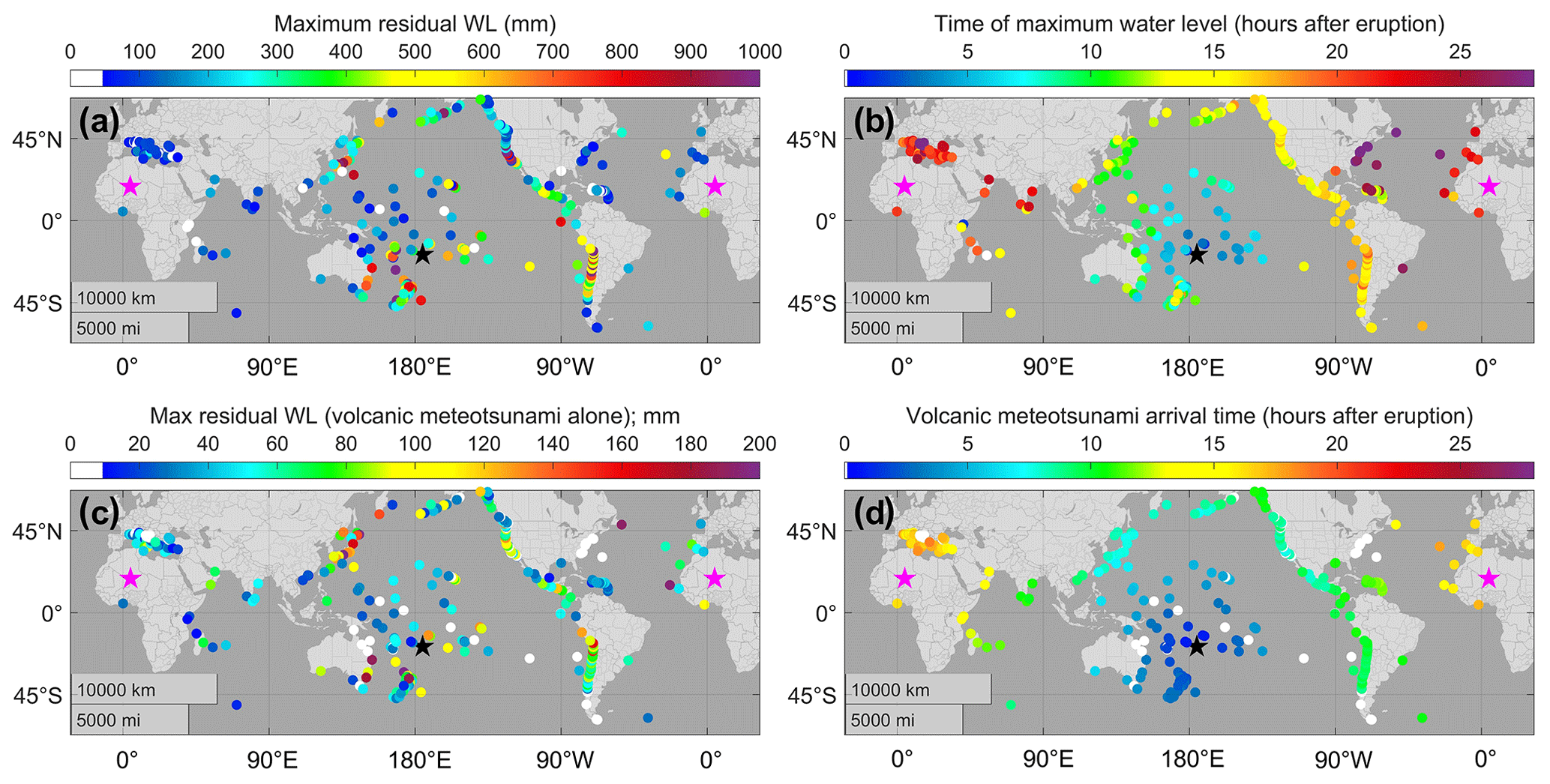
Figure 1Tonga tsunami global manifestations: (a) maximum amplitude of combined volcanic (VMT) and marine tsunamis, (b) time of maximum amplitude, (c) first arrival VMT amplitude, and (d) VMT arrival time. White markers in (c) and (d) indicate locations where meteotsunami properties could not be determined. The locations of the eruption and its antipode are shown by black and magenta stars, respectively. Maps made in MATLAB using data from Natural Earth.
Several Indian Ocean tide gauges (East Africa, Oman, Sri Lanka, and India) show WL changes shortly after the atmospheric waves arrived but display little evidence of a marine tsunami. In the Atlantic Ocean, there was a strong signal in Senegal, Ghana, and in the Cabo Verde, Canary, and Azores islands. The Azores showed a large WL amplitude (∼ 0.6 m), but this area is undergoing volcanic activity with frequent seismicity. While no nearby air pressure record is available to confirm a relationship to the meteotsunami wave in the Azores, no strong seismic activity was recorded either; hence, the causality of this result is uncertain. All of these gauges are located within ∼ 3000 km of the antipode of the Tonga event (20.54∘ N, 4.62∘ E in the Sahara), where the concentric shock waves re-converge. The resulting interference pattern may have increased the magnitude of atmospheric waves in some places and the subsequent VMT and masked others.
In the eastern North Atlantic, small tsunamis occurred after the second pass of the VMT wave on 16 January, e.g., at St. Johns, Canada (∼ 0.2 m). Storminess after 16 January precluded further detection there and in the Baltic Sea; and little or no signal was seen on the European Atlantic coast at any time. Widespread VMTs occurred in the Caribbean and Mediterranean seas, the latter being close to the antipodal point of the shock wave. In both regions, successive occurrences of the VMT wave have different impacts on WL variability.
These results suggest that VMT characteristics vary between closely spaced stations because of local bathymetry, ambient currents, and the orientation relative to the source (Šepić et al., 2015; Garrett, 1970; Williams et al., 2021). The VMT properties also change with atmospheric stratification and due to dispersion as the shock wave propagates; the directionality of the VMT (towards or from land) also matters (Garrett, 1970). Thus, the level of response from a VMT event is locally variable, despite its global reach.
4.2 Tsunami propagation in the Pacific as determined from deep-water buoys
The network of the National Data Buoy Center (NDBC) deep-water tsunami warning buoys provides significant spatial coverage of the Pacific and can reveal the offshore characteristics of strong oceanic signals like tsunamis (e.g., surface amplitude) without contamination by surface swell. These buoys generally provide a 15 min temporal resolution but, when triggered by large signals, record 1 min data. We examined all available buoys but found that many buoys did not record any data at all during the Tonga event. Thirty NDBC buoys in the Pacific recorded at least part of the marine tsunami; however, only a subset caught the VMT (12 buoys). Locations are given in Fig. 2a and details of the buoys are given in Table S1. Ten locations measured the VMT in the western Pacific, one in Alaska, one in Hawai'i, and none in the eastern Pacific. The western Pacific data reveal a similar spike-like waveform, with a steep rise followed by a rapid decrease. The magnitude of the VMT-induced WL response is nearly consistent across the basin, except at two of the nearest buoys to Tonga (55015 and 51425), where amplitudes were larger, 70 and 58 mm, respectively. All other VMT magnitudes were between 25 and 40 mm, independent of distance from Tonga (Fig. 2b).
The energy generated by the Tonga tsunami may have been sustained by repeated returns of the atmospheric wave at many locations. Can the spatial characteristics of energy decay be suggested from the limited buoy data? We next make an estimate of the “persistence” of the tsunami in the Pacific by determining the length of time (in hours) that the buoys were triggered in each region of the Pacific for 1 min resolution observations. This metric, possibly influenced by instrumental noise (or gauge problems) at some locations, allows a simple, if imperfect, estimate of tsunami energy decay for individual buoys and for regional averages. We omit buoy 52406 (which recorded at high resolution for >30 h, for reasons unclear) and determine a median regional persistence in the southwestern Pacific (i.e., the buoys nearest to Tonga) of 9 h, while the buoys immediately west of Tonga had a median regional persistence of 6.5 h. At the periphery of the Pacific, the median regional persistence was 610 h in the northwestern Pacific (Japan and surrounding areas), 9 h in the northern Pacific (Alaska), 10 h in the northeastern Pacific (California–Canada), and 13 h around South America. Thus, we generally see a longer persistence in far-field Pacific regions than in near-field regions (Fig. 2c). The maximum VMT magnitude (where detected) and the persistence times at all buoys are given in Table S7.
A subset of five buoys provides an effective summary of the VMT behavior in deep water (Fig. 2d). Two buoys (52402 and 21420) are close to being a great circle with each other and the Tonga eruption; buoy 52402 is ∼ 5000 km from Tonga, while 21420 is ∼ 2700 km further towards the southern coast of Japan. The VMT maximum WL at the first buoy is about 38 mm vs. 30 mm at the second; the subsequent WL oscillations at both buoys are similar in form. This suggests that the VMT response of the marine WL decayed very slowly, at least across the Pacific basin. The full set of WL responses at all buoys is given in the Supplement and compared by region (Figs. S13–S18).
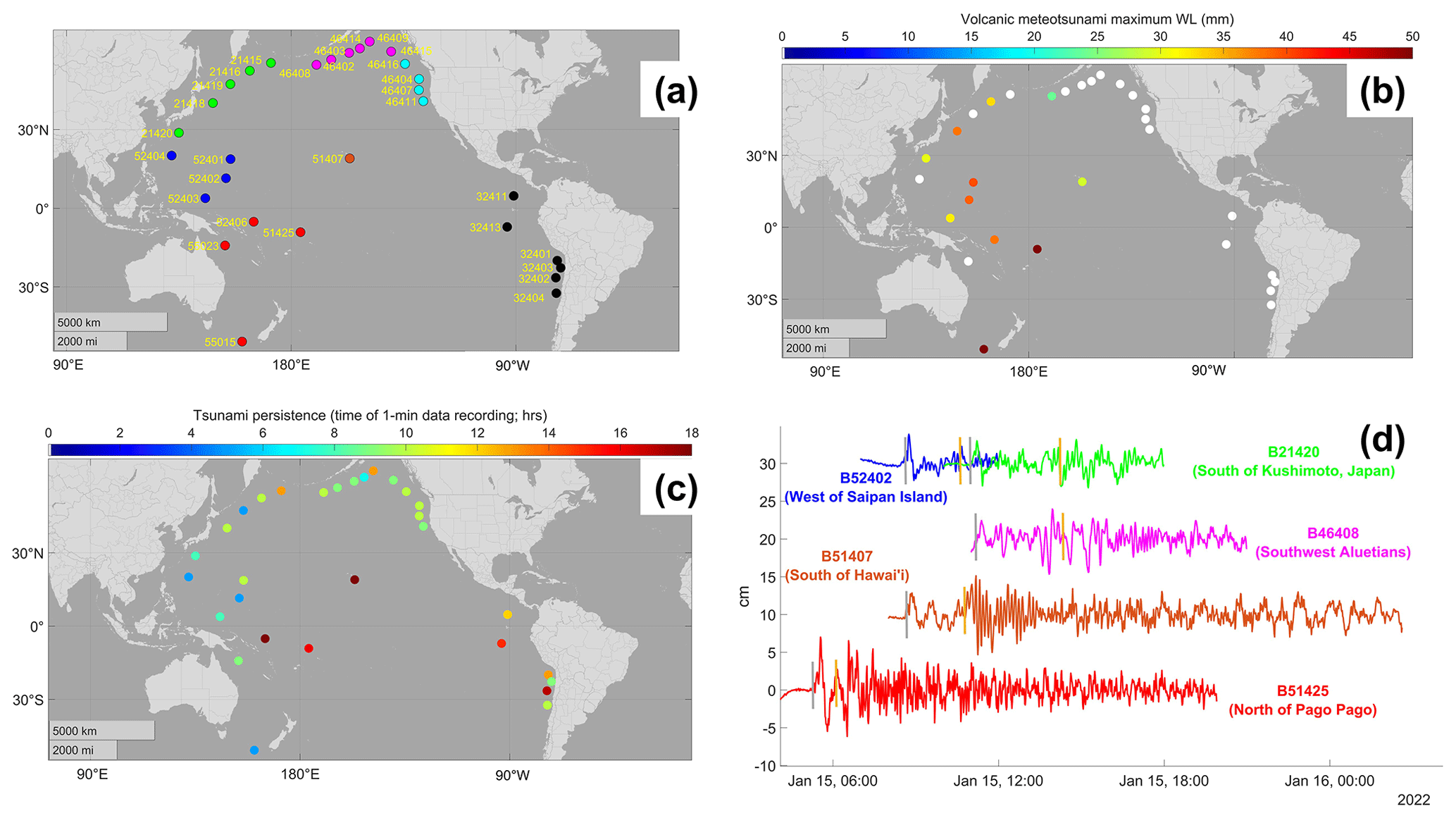
Figure 2Pacific deep-water NDBC buoys used to detect the VMT and marine tsunami of the Tonga event. (a) Buoy locations and NDBC buoy designation numbers (Table S1), with colors used to show Pacific regional delineation (red: southwest; orange: central; dark blue: west; green: northwest; magenta: north; cyan: northeast; black: southeast). (b) Maximum VMT-induced WL (mm) detected at each buoy according to color scale at top of map. White markers indicated that the VMT was not detected at the buoy. (c) Persistence time of the tsunami signal at each buoy, representing the length of time that each buoy recorded at 1 min resolution (h). (d) WL response to the VMT and marine tsunami at five deep-water buoys in the Pacific using same color scheme as (a). Two buoys are given on the same line (B52402 and B21420) since their physical locations were on nearly the same great circle path from Tonga; other buoys are offset 10 cm vertically from each other. VMT arrivals based on a theoretical travel time of 1115 km h−1 are indicated by gray vertical lines, and marine tsunami arrivals based on an average travel time of 700 km h−1 are indicated by orange vertical lines. Maps made in MATLAB using data from Natural Earth.
4.3 Coastal characteristics of VMTs
As the VMTs propagated from deep water to the coast, we observed several cases in which an abrupt change in geometry produced a large amplification. We return to the example of buoys 52402 and 21420 discussed above, and now compare data from the buoy closer to Japan (21420) with the nearest coastal tidal gauge that also has PA data, Kushimoto, Japan (Fig. 3). The first Lamb wave with a pressure change of ∼ 0.6 mb occurred at ∼ 11:30 UTC on 15 January at Kushimoto (Fig. 3a, c). The WL response in the PB record (a positive ∼ 30 mm spike then a ∼ 30 mm negative one) is direct and presumably represents the forced wave. We compare the two closest PA records to the PB data (Aburatsu and Kushimoto; see Appendix A for details). Longwave celerity at the buoy depth of 5700 m is 850 km h−1; , relative to the observed amplification of α≅4. The CWT scalogram in Fig. 3e shows the WL response to the shock wave at ∼ 10 h post-eruption as two relatively distinct bands of energy with periods of ∼ 1 h and 5–10 min; these fade within ∼ 1.5 h.
Kushimoto WLs effectively illustrate the potential for amplification of VMTs. The first (VMT) waves arrived between 12:00 and 14:50 UTC (Fig. 3b, d), prior to the marine tsunami at about 14:50 UTC; their period is ∼ 0.3 h (Fig. 3f). Shorter-period energy is seen only after the arrival of the marine wave. The initial positive VMT amplitude of ∼ 210 mm is a response to the atmospheric shock wave and represents an amplification factor of ∼ 7 relative to the forced wave and β∼35 relative to the VMT magnitude, for which the inverse barometer response would be only 6 mm. Apparently, the Japan trench with depths to 8 km (an≈5.5) and continental shelf between buoy 21420 and Kushimoto allowed considerable growth of the forced wave relative to Fig. 3a and c. A large volcanic explosion (such as Krakatoa) could yield a shock wave with a magnitude of 30–60 mb (Schufeldt, 1885), which could potentially drive a large VMT at this location before the arrival of the marine tsunami.
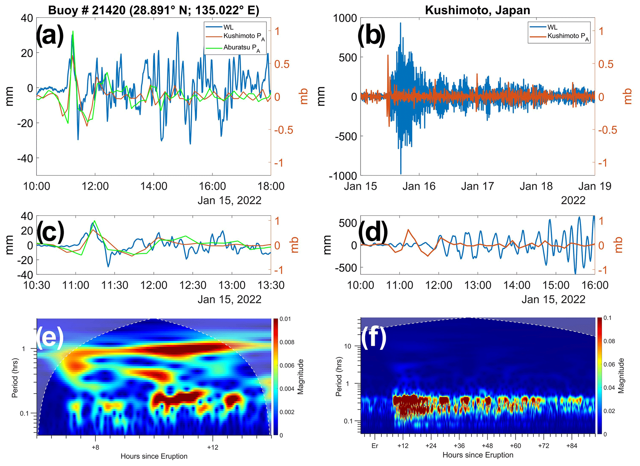
Figure 3Tsunami response at NOAA PB buoy 21420 and a coastal tide gauge (Kushimoto, Japan): (a) residual PA at Kushimoto (orange) and Aburatsu (green), and detided residual buoy WL (blue) with PA records shifted plot 26 and 16 min to account for distance from the buoy (see Appendix A for details); (b) PA (orange) and detided residual WL (blue) at Kushimoto; (c) expanded view of (a) showing arrival of a VMT as a supercritical forced wave at 11:50 UTC ahead of the marine tsunami wave at 14:50 UTC (c); (d) expanded view of (b) showing the arrival at Kushimoto of the VMT as a subcritical free wave at 12:00 UTC; (e) buoy residual WL CWT scalogram, 6–14 h after the eruption; (f) Kushimoto WL CWT scalogram for 92 h after the eruption.
Observations near Hilo, Hawai'i, show similar phenomena to those observed at Kushimoto (Fig. 4). We use NOAA tsunami bottom pressure (PB) buoy 51407 in 4.7 km water depth south of Hilo combined with atmospheric pressure (PA) and WL data from Hilo (NOAA station 1617760). Figure 4a and c show PA and PB data (converted to WL). Despite the distance (∼ 100 km) between the two records, the WL and PB responses are almost simultaneous, at 08:54 UTC. The first PA pulse of ∼ 1.5 mb elicits a WL response of ∼ 30 mm (α∼2) of the same sign as expected for a supercritical wave and similar to the response at Kushimoto. This modest amplification is still slightly larger than expected for an∼1.2. Smaller positive WL pulses follow the first; after the third, these pulses are overlain by the beginnings of the marine tsunami signal at ∼ 10:30 UTC. These may be a soliton train, as predicted by the nonlinear theory (Pelinovsky et al., 2001). The CWT scalogram in Fig. 4e shows that marine tsunami waves with periods of 0.15–0.2 h arrived at buoy 51407 before 11:00 UTC; shorter waves (periods <0.1 h) arrived later, confirming the weakly dispersive character of waves in the tsunami band. The VMT is also clearly visible. It appears just before 09:00 UTC as a broadband signal with periods of 0.4–1.1 h. Over time, the pulse shifts to higher frequencies and then disappears by ∼ 12:00 UTC.
The detided residual WL data at Hilo present quite a different appearance from the offshore PB data (Fig. 4b, d). The first wave arrival (∼ 120 mm) occurs at 09:28 UTC (∼ 1 h after the PA spike) with a negative excursion rather than a positive one. This is followed by a series of smaller oscillations leading up to the arrival of the marine tsunami at about 11:37 UTC. The forced wave is not evident, and the early arriving VMT waves at Hilo are likely free waves that have propagated around the island on which Hilo sits and then amplified, having been generated at the abrupt rise of the island platform; the total amplification is β=9. The waves from the marine tsunami wave reach ∼ 400 mm, which represents an amplification factor of about 5 relative to the same PB waves at the buoy. Records from nearby Hawaiian gauges show similar features. The CWT scalogram for Hilo WL in Fig. 4f emphasizes the absence of longer-period tsunami waves with periods around 1 h. Instead, the weak VMT WL response is followed by waves with similar periods, ∼ 0.15 to 0.7 h. Over the next several days, the oscillations weaken, with the shortest period waves disappearing first. Hilo is well known to be resonant to tsunamis, and our observations may be related to quarterwave resonance (Pattiaratchi and Wijeratne, 2015; Tang et al., 2017). However, water levels at other Hawaiian tide gauges behaved similarly to Hilo.
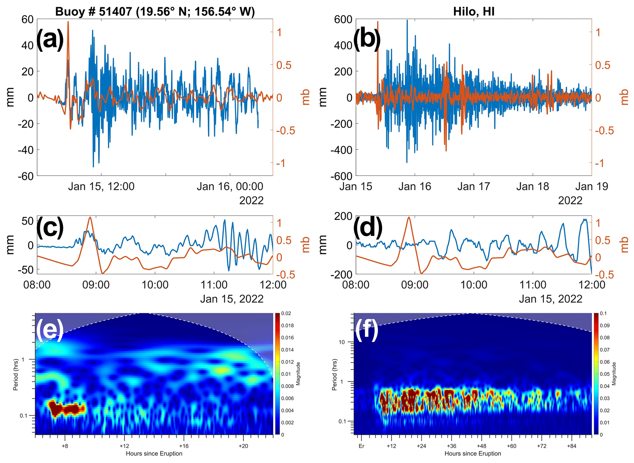
Figure 4Comparison of WL (blue, mm) and PA (orange, mb) at offshore buoy 51407 and Hilo, HI. (a) PA at NOAA tide gauge 1617760 Hilo, HI, and detided WL residual from NOAA PB buoy 51407 south of Hawai'i following the Tonga event; (b) PA and detided residual WL (blue) at Hilo; (c) expanded view of (a) showing the arrival of the VMT at buoy 51407 in the form of a supercritical forced wave at 08:54 UTC ahead of the marine tsunami wave arrival at ∼ 10:54 UTC (c); (d) expanded view of (b) showing the arrival at Hilo of the VMT in the form of a subcritical free wave at 09:28 UTC; (e) a CWT scalogram of buoy heights from PB for 6–24 h after the eruption; (f) a CWT scalogram of WL measured at Hilo for 92 h after the eruption.
Kushimoto and Hilo are only two examples of VMT effects in the Pacific. The VMT-induced WL magnitudes were similar to Kushimoto at other Japanese locations and were 50–210 mm in New Zealand and eastern Australia. Much smaller (∼ 20 mm) VMTs were seen in the South China Sea, though 1 min data were available at only two locations (Hong Kong and Shenzhen; Wang et al., 2022). In the eastern Pacific, distant from Tonga, VMT waves arrived 3.5 (California) to 5 h (Chile) before the marine tsunami, allowing their WL effects to be easily distinguished (Fig. 1a, c, Table S3), and both regions had particularly large maximum tsunami magnitudes (positive and negative swings). Air pressure (PA) spikes of ± 0.6–0.7 mb and +1.5 and −0.8 mb at Port San Luis, CA, and Coquimbo, Chile (Fig. 5), led to wave excursions of +110 and −150 mm, respectively, with total amplifications of β ∼ 15–25 at Port San Luis (Fig. 5c) and ∼ 6 (positive wave) and 30–40 (negative wave) at Coquimbo (Fig. 5d). There were at least six arrivals of the shock wave over 3 d. This recurrence, coupled with very long decay times (below), caused WL disturbances to continue for >90 h, emphasizing the role of the VMT in recharging the combined marine and volcanic tsunami (Fig. 5e–h).
These Pacific examples demonstrate combined marine and VMT impacts; in other regions, the VMT occurs in isolation. At Charlotte Amalie in the Caribbean (Fig. 6), the PA spikes and resulting VMTs are well correlated (Fig. 6a). The first PA spike of ∼ 1.2 mb led to waves of 80 mm about 1 h later, apparently from the free wave (Fig. 6b). In contrast, the third PA spike of ∼ 0.5 mb apparently excites a forced wave with amplitude of about 50 mm, simultaneous with and of the same sign as the PA fluctuations (Fig. 6c). Waves arriving 1 h later and presumably representing the free wave were larger, ∼ 80 mm, giving . The fourth PA spike mb again excited a forced plus free wave response, with the later waves being as large as ±100 mm (Fig. 6d). This corresponds to an impressively large . The CWT scalogram shows that the water level in this harbor responds most strongly at periods of ∼0.5 to 0.9 h (Fig. 6e). The CWT of PA at Charlotte Amalie shows eight spikes at ∼12 h intervals, suggesting that the shock wave circled the planet at least four times over 4 d (Fig. 6f; see also Fig. 5g). The largest WL response occurred from the fourth VMT (Fig. 6e, f) for yet unknown reasons. Other gauges in the Caribbean showed significant VMT effects (Fig. S11) that were strongest on the second or third pass of the atmospheric disturbance. While β varies with the event, there are numerous volcanoes in the Caribbean, and severe tsunamis (both VMT and marine) could be a very real hazard in locations where amplification occurs.
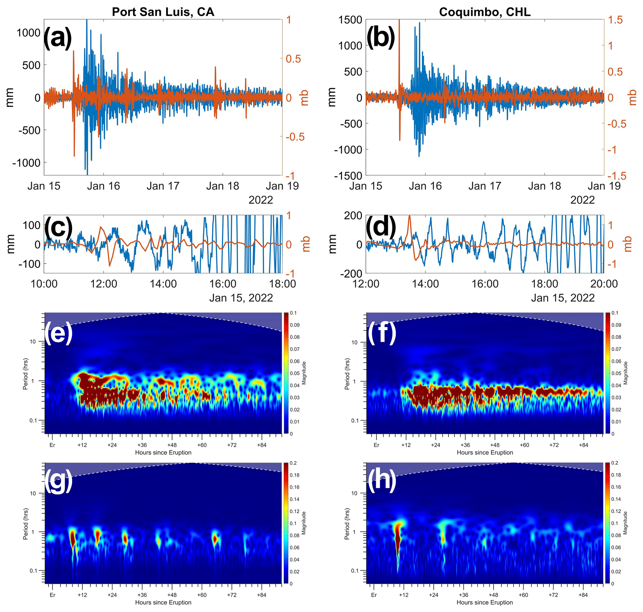
Figure 5Residual WL (blue, mm) and detrended air pressure (orange, mb) at (a) Port San Luis, California (NOAA Station 9412110), and (b) Coquimbo, Chile; panels (c) and (d) show expanded views of panels (a) and (b) of the WL and PA records showing the initial arrivals of the VMT and marine tsunami as well as scalograms from CWT analyses of WL in (e) and (f) and for PA in (g) and (h). Vertical scales in (c) and (d) are set to a small range to highlight the VMT impacts.
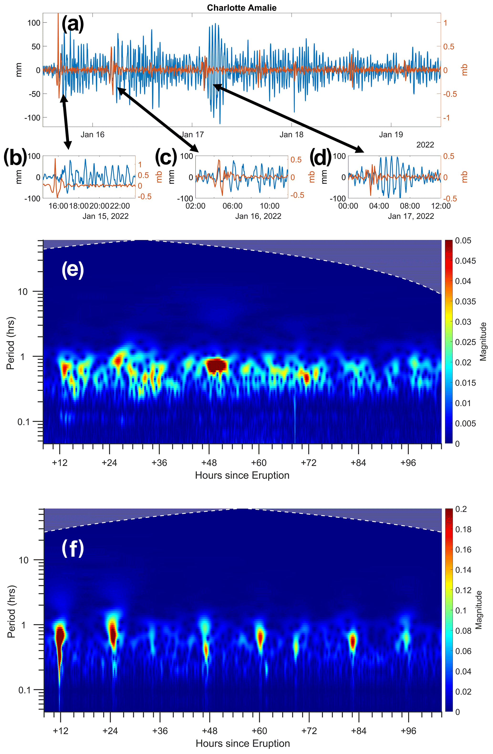
Figure 6VMTs at Charlotte Amelie (NOAA gauge 9751639) in the Caribbean: (a) residual WL variability (blue) and PA (orange) from 15:00 UTC to 19 January 2022; (b–d) expanded views of (a) at the times of the first, second, and fourth PA spikes; (e, f) CWT scalograms of the WL and PA records in (a).
The shock wave magnitudes were generally smaller in the Mediterranean than in the Caribbean, perhaps because of the greater distance from Tonga and the complex land topography in the region. Still, VMT-induced meteotsunamis were measured at many locations; they were largest in Sicily, Sardinia, and the “boot” of Italy. Because this region is close to the antipode, the first PA waves arrived from opposite directions only a few hours apart, at ∼ 20:00 and 23:30 UTC on 15 January. The propagating waves produced multiple waves rather than a clear PA spike that swept across the region. A weaker group of waves occurs 38 h later at ∼ 12:00 UTC on 16 January, followed by a third group at ∼ 00:00 UTC on 19 January, not seen at all stations. Water level records usually show a single, long-lasting event following the first PA packet arrival, with muted responses for the second and third packet. The largest tsunami amplitude, ∼ 300 mm (Fig. S12), occurred at Crotone, Italy, after a steady build-up from the VMT arrival. At a small number of stations, e.g., Cagliari, Italy, there were multiple VMTs, as in the Caribbean (Fig. S11). Finally, a few locations in the Adriatic Sea had no response to the first wave packet but responded strongly to the second VMT, with β ≈ 8–13. Thus, the discrete response of WLs to individual shock waves is not as clear in the Mediterranean as in the Caribbean, though repeated passes of the shock wave lead to sustained WL variability.
4.4 Energy decay
The Tonga event released significant energy and its tsunami persisted longer in the Pacific than other recent marine tsunamis. Our estimate of energy Eo for the Tonga event (0.0096 m2, N=37) is comparable to the Chilean event (0.01 m2; N=28) and about 3.8× less than the Tohoku event (0.036 m2; N=40). Previous estimates for the Chilean and Tohoku events were 0.009 and 0.032 m2, respectively (Rabinovich et al., 2013). Decay timescales for the Tonga event varied from 29–44 h in Alaska, 25.4 h (Santa Barbara) to 37 h (San Diego) on the US West Coast, and 22.2 h (Nawiliwili, Hawai'i) to 29.3 h (Pago Pago, Samoa) for island stations (Fig. S19). The Tonga decays are notably longer than other events, especially in Alaska and (most) California locations. The differing timescales between stations depend on distance from the event, frequency content (high frequency decays more quickly), and shallow water processes (Rabinovich et al., 2013). Our estimated median td values for the Tohoku, Chile, and Tonga events are 26.6±2.4 h (N=40), 27.6±2.8 h (N=27), and 31.0±2.6 h (N=37), respectively (Fig. 7). Previous estimates for the Tohoku and Chilean events were 24.6 and 24.7 h. The longer decay time of the Tonga event emphasizes the importance of the VMT. Though the VMT was smaller than the marine tsunami, it was refreshed by the Lamb waves that repeatedly circled the planet (see e.g., Fig. 5g). The long energy decay scales calculated for the northern Pacific are in line with our simple estimates of decay taken from the buoys, which were longest in the northern/northeastern Pacific and near Tonga (e.g., Hawai'i and Pago Pago; see Sect. 4.2).
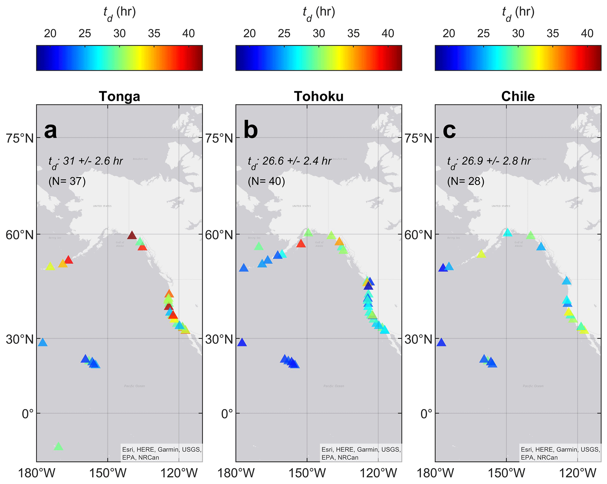
Figure 7Decay timescales (hours) of recent tsunami events at NOAA gauges in the northern Pacific, showing (a) Tonga, (b) Tohoku, and (c) Chile. Median td, errors, and number of stations used are given in each panel.
4.5 Amplification, β
Amplification β is a vital indicator of possible future VMT hazards and vulnerability. It was calculated for ∼ 75 % of all tide-gauge locations where the shock wave was detected in a nearby PA record (Tables S5 and S6). Clearly, β is highly local, with strong spatial heterogeneity (e.g., Fig. 8). Maximum values of 15–35 were measured at 26 stations in all regions, and over 50 locations had β>10 (Fig. 8a–d). The largest values of β are observed in Japan, the northeastern Pacific, New Zealand and Australia, and the Caribbean. Wherever high β values are observed near an active volcano, there is the potential for a large VMT. Note that β values are uncertain by ∼ 30 % (see Appendix A), mainly due to the uncertainty of PA observations which have low amplitudes and coarse temporal resolution.
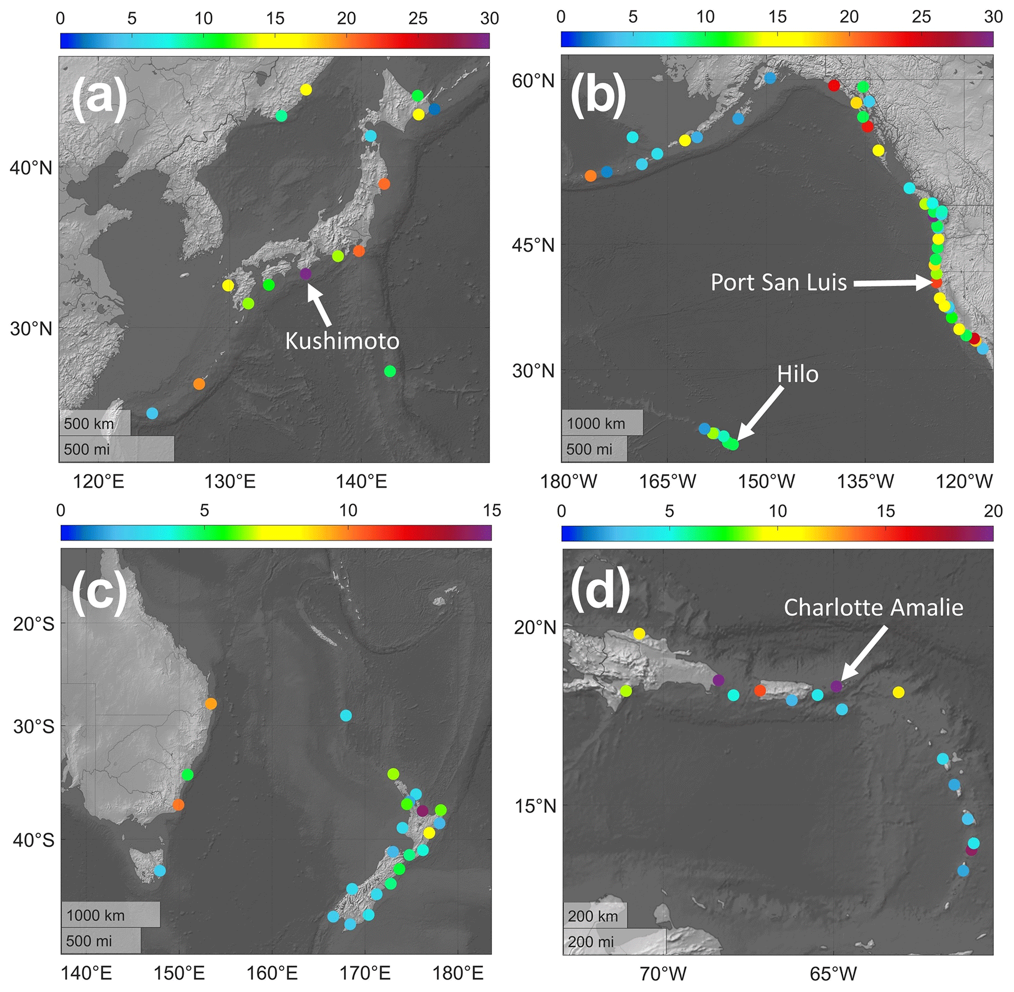
Figure 8Amplification, β, in (a) Japan, (b) the northeastern Pacific, (c) New Zealand and Australia, and (d) the Caribbean. Locations of note with large amplification which were discussed above are indicated: Kushimoto (Fig. 3), Hilo (Fig. 4), Port San Luis (Fig. 5), and Charlotte Amalie (Fig. 6). Note diverse color scales. Maps made in MATLAB using data from Natural Earth.
Analyses of high-resolution WL data from tide gauges (with local PA, where possible) provide an unprecedented global view of a volcanic meteotsunami (VMT) acting together with a marine tsunami. A moderate marine tsunami was measurable at nearly all Pacific Ocean tide gauges and deep-water buoys but at only a few stations elsewhere. In addition, most tide gauges and about half of the deep-water buoys also observed the VMT. In the North Pacific, wave amplitudes and energy were comparable to the Chilean event. Out of 308 tide gauges, 10 showed a total VMT amplification (β) of >20, 54 were >10, 113 were >5, 204 were 2 or more, and 230 were 2 or less; the remainder did not register any detectable VMT signal. Hence, significant amplification is a localized, but still potentially important, process. We note that much of the world's coastline is still not gauged, and there are many locations in which the VMT was amplified but not measured, e.g., Lima. Thus, the Tonga event tsunami was “global” because of the reach of the VMT and its impacts on WLs.
In the Pacific, the VMT preceded the marine tsunamis by up to 5 h and the two together produced observable perturbations in water levels for more than 3 d after the eruption. The effects of atmospheric gravity waves were observed in ocean bottom pressure data after the arrival of the Lamb waves and before the marine tsunami arrived. However, we observed a delay (∼ 1–2 h) of the water level response to the shock wave at coastal tide gauges. This delay may be related to the “sequencing” of tsunami waves and observations that the first wave of a tsunami is not always the largest (Okal and Synlokas, 2016). However, this suggestion is based on “traditional” seismic tsunamis; it is not clear if VMTs follow exactly the same physical dynamics.
How can we place the Tonga event in a larger context? This event drove VMTs no larger than ∼ 210 mm in the far field due to shock wave magnitudes of ∼ 0.5 to 5 mb. However, the total amplification, β, varied from ∼1 to 35×. Values at the larger end of this range were mainly seen at coastal locations; island locations typically had β<5, with only a few exceptions (e.g., Hawai'i and Naha). The reasons why certain regions exhibited a larger amplification (e.g., β) than others, and the possible role of bathymetry, remain to be understood, e.g., through model studies like Denamiel et al. (2023). It seems likely, however, that locations with an ocean trench between the source and the coastal station are at particular risk; this is typical for much of the Pacific “Ring of Fire”, as conceptualized in Fig. 9. We assume a 5 mb Lamb wave traveling over deep water which initially induces a forced wave WL fluctuation of 60 mm. After traveling some distance, the forced wave grows 4-fold. The trench, with FA near unity, increases VMT amplitude even if the trench is narrow relative to the wavelength of the longer-period tsunami components. Coastal and harbor processes, which can vary substantially along a coast, provide a further boost. Taken together, these processes can cause an amplification of up to β=36 (as suggested in Fig. 9), in which case an initially modest (5 mb) PA spike and corresponding WL fluctuation of 6 cm can become a ∼ 1.8 m tsunami.
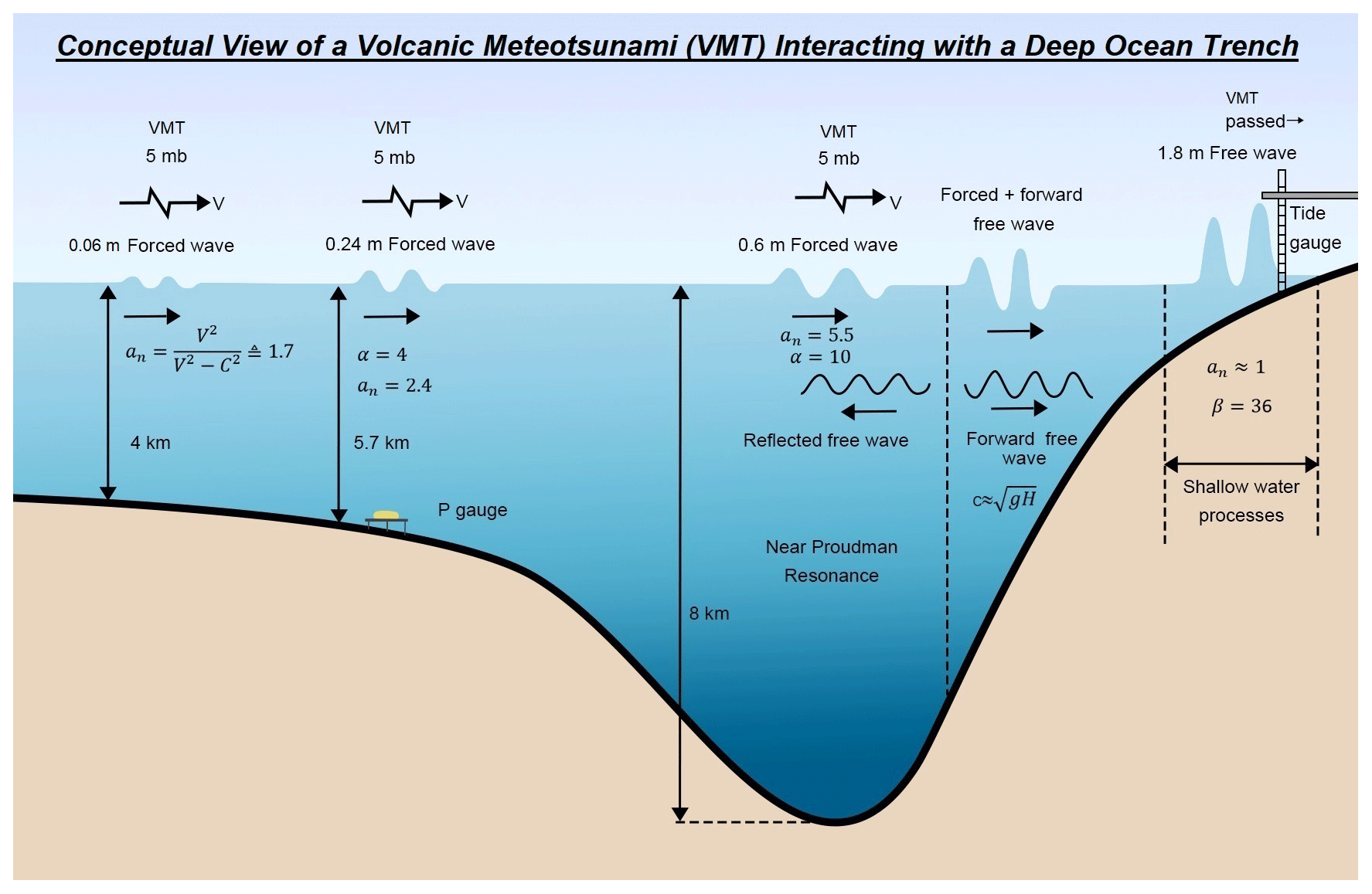
Figure 9Conceptual view of amplification of a VMT, based on Tonga event observations. An initial shock wave amplitude of 5 mb is amplified by Proudman resonance in the trench and again by shallow water processes, after reflection of a free wave by the steep topography landward of the trench. With β=36, a 1.8 m tsunami occurs at the tide gauge. A larger VMT would lead to a proportionally larger response.
The VMT from the Tonga event was small, but β was >10 in many parts of the world with active volcanoes, including Italy, Alaska, Japan, and New Zealand. A much larger VMT can occur close to a VEI 6–7 volcanic explosion. For example, in 1883, ship barometers measured fluctuations of 1–2 in. of mercury (30–60 mb) near Krakatoa (Symons, 1888). Taking 30 mb as a conservative upper limit for a VEI 6 event and β=10 to 35, a VMT of 3.5 to ∼ 10 m is possible. In most cases, this would be later followed by larger water waves, but the rapid arrival of VMT waves of this size could be catastrophic and might occur in some locations without being followed by a marine tsunami. Moreover, Krakatoa is not the largest historical event by any means – the Santorini (∼ 3600 year BP) and Tambora (1817) events were much larger (Newhall and Self, 1982), but these events lack data regarding VMT impacts.
Present-day warning systems are designed for marine tsunamis and do not generate timely warnings for meteotsunamis of any origin as noted by Vilibić et al. (2016). Future warning systems should consider both marine and meteotsunamis, but this is not straightforward because of differences in the causation and warning times between weather and volcanic meteotsunamis. Weather conditions for meteotsunami genesis, which evolve over days, may be able to be at least partially predicted, and this threat is confined to specific regions. Volcanic eruptions are a different problem. The VMT threat is global; VMTs can cross an ocean basin in a matter of hours, given the rapid shock wave celerity (∼ 1100 km h−1), and their magnitude can be larger. Thus, though VMTs occur only infrequently, the possible hazard deserves further consideration.
We conclude the following regarding the volcanic meteotsunami (VMT) from the Tonga event.
-
The VMT arrived before the marine tsunami at all stations where both were observed, though the marine wave was larger at stations where both occurred.
-
The atmospheric shock wave transited the globe multiple times; on every pass, it imparted additional energy to WL fluctuations which sustained or re-excited the VMT, likely contributing to a ∼ 25 % longer decay timescale than for recent marine tsunamis generated by earthquakes.
-
The refocusing of the shock wave in the atmosphere near the antipode of the eruption may have increased tsunami amplitudes in Africa and the Mediterranean. The reasons for the strong Caribbean response are yet unclear.
-
The first wave observed at deep-water pressure gauges was the supercritical VMT-forced wave predicted by theory, but at most tide gauges only the subcritical free wave response was observed.
-
The nominal amplification, an, shows that deep water allows strong growth of the forced wave beneath a VMT (Proudman resonance). The large total amplification, β, at Japanese coastal stations suggests that deep-water trenches around the Pacific “Ring of Fire” (with its many volcanoes) and elsewhere may produce the potential for large, consequential VMTs.
A1 Data inventory
We acquired 1 min resolution data from the following sources: the European Commission (EC) World Sea Levels Database (https://webcritech.jrc.ec.europa.eu/SeaLevelsDb/Home, last access: 30 August 2022), the Intergovernmental Oceanographic Commission (IOC) sea-level station monitoring facility (https://www.ioc-sealevelmonitoring.org/, last access: 30 August 2022; VLIZ, 2022), the National Oceanic and Atmospheric Administration (NOAA) CO-OPS Tides and Currents tsunami warning network (https://tidesandcurrents.noaa.gov/tsunami/, last access: 30 August 2022), and Land Information New Zealand (https://www.linz.govt.nz/sea/tides/sea-level-data/sea-level-data-downloads, last access: 30 August 2022), plus data obtained by direct communication from the National Institute of Water and Atmospheric Research (NIWA) of New Zealand (https://niwa.co.nz/our-services/online-services/sea-levels, last access: 30 August 2022). Other stations from these networks with less frequent data were used when 1 min data were not available. Tidal predictions and residuals are provided in the EC and NOAA databases; however, a tidal signature or a slope sometimes remains in the provided residuals, and the IOC and NIWA data do not provide any predictions. Therefore, we apply an EEMD analysis (Huang et al., 1998) to all WL data to remove low-frequency components and biases in mean water level to yield data in which the tsunami signal is dominant.
Air pressure (PA) records at 1 min resolution are downloaded from the Chilean Meteorological Directorate (CMD; https://climatologia.meteochile.gob.cl/, last access: 30 August 2022), the Australia Bureau of Meteorology (BOM; http://www.bom.gov.au/climate/data/, last access: 30 August 2022), and the Instituto Superiore per la Protezione e la Ricerca Ambientale (ISPRA; https://www.mareografico.it/, last access: 30 August 2022) network for Mediterranean locations, 6 min PA data are downloaded from NOAA at tide gauges and PB data from offshore buoys in the Pacific and Caribbean (https://tidesandcurrents.noaa.gov/stations.html?type=Meteorological+Observations, last access: 30 August 2022; https://www.ndbc.noaa.gov/obs.shtml, last access: 30 August 2022), and 10 min PA data are acquired from the Japan Meteorological Agency (JMA; https://www.data.jma.go.jp/obd/stats/etrn/index.php, last access: 30 August 2022) and the National Institute of Water and Atmospheric Research National Climate Database (NIWA/NCD; https://cliflo.niwa.co.nz/, last access: 30 August 2022). A total of 137 air pressure locations were used, listed in Table S5.
Finally, we download data from 30 Pacific deep-water buoys (see Table S1) from the National Data Buoy Center (NDBC; https://www.ndbc.noaa.gov/obs.shtml, last access: 30 August 2022) tsunami warning center operated by NOAA; these provide 1 min data during “active” WL events and 15 min data otherwise. Other buoys were investigated, but because the buoys only sometimes operated at 1 min resolution, many were not triggered until the VMT wave had passed; thus, it was most often not captured. All buoy data and air pressure data were conditioned using EEMD as described above.
A2 Water level (WL) analysis
The VMT magnitudes and arrival times, as well as the amplitudes of the largest positive and negative tsunami waves at each location, are determined from the WL residuals via numerical and visual estimation of the residual time series. The first arrival times and amplitudes represent the effects of the VMT, which travels faster than the marine tsunami; times are determined by finding the rising edge of the first obvious anomalous wave in the residual WL time series, and the VMT amplitude is defined as the maximum WL immediately after the first arrival (Table S3). At a small number of locations, the VMT wave could not be clearly observed, as noted in Table S3 and in Fig. 1c and d. We compare the distances and first arrival times at all tide-gauge stations via robust regression (Holland and Welsch, 1977) and find an estimate of the VMT velocity from the slope of the regression as 1054±7 km h−1 (Fig. S11b), slightly less than that estimated from the air pressure gauges (1115±3 km h−1; Fig. S11a). These estimates can be compared to the much slower celerity estimate for the water wave component of the tsunami (708±8 km h−1; Fig. S11c), clearly demonstrating that the first arrival WLs are due to the VMT. Note that the water wave celerity corresponds to an average water depth of about 5 km.
The timings and amplitudes of the largest positive (negative) waves due to the marine tsunami are determined by when the first local maximum (minimum) occurs after the first arrival of the tsunami. At some locations, slightly larger amplitudes are seen many hours later, usually on the following tidal cycle (i.e., “tidal pulsing”), while other locations have the largest wave arriving a few oscillations after the arrival; the latter may be due to the issue of “sequencing” as described by Okal and Synolakis (2016). The WLs and times for maximum WLs, as well as the differences between extreme levels and the VMT arrival, are given in Table S2 and Figs. 1a and c, S5, and S6, and the same parameters for minimum WL are provided in Table S4 and Figs. S7 and S8. The time differences between first arrival and maximum/minimum WLs are shown in Figs. S9 and S10. Determination of VMT (“PA spike”) amplitudes was carried out in the same manner as for the tsunami amplitudes.
A3 Air pressure gauge choices for Kushimoto
Comparison of the Kushimoto tide-gauge WLs to offshore buoy 21420 and air pressure (Fig. 3) raises the difficulty that there is no PA station within more than 300 km of the buoy; therefore, we use the two nearest. Aburatsu (∼ 465 km) is on a direct line from Tonga and the buoy, while Kushimoto is 305 km from the circle centered on Tonga through the buoy. Accounting for the distance between the coastal gauges and the buoy using a shock wave velocity of 1092 km h−1 (Table S3), we shift the time index of the PA records by 16 and 26 min, respectively. Both PA records are used because the sparse, 10 min resolution of the PA records precludes either from completely capturing the VMT.
A4 Energy decay analysis
Following Rabinovich (1997), we detide 1 min NOAA WL data, remove any residual trend, and then produce power spectra for 4 h segments of the WL residual, with an overlap of 2 h between successive analyses. A multi-tapered method (McCoy et al., 1998) was applied because it reduces noise and edge effects but still conserves energy. The energy within the tsunami band (between 10 min and 3 h) was then integrated for each 6 h period and an exponential decay model of form applied, where Eo is the peak energy in the fit and td is the e-folding (decay) timescale. To account for the initial “diffusion period” (Van Dorn, 1984, 1987), the two initial, largest energy values were removed; hence, Eo represents the energy at the commencement of exponential decay. The exponential decay was fit to all tsunami-band energy values until measurements dipped below the noise floor. The noise floor was defined as the 80th percentile energy in the tsunami band from 7–12 d after the event. Each fit was examined for validity, and the range of points in the fit was manually adjusted in five cases. For fits for which the standard error in the coefficients was more than 20 %, the coefficient value was removed. The analysis was applied to four events: the 2009 Samoa tsunami, the 2010 Chilean tsunami, the 2011 Tohoku tsunami, and the 2022 Tonga tsunami. However, due to the low energy of the Samoa event, we focus primarily on the other three. In our analyses, we also distinguish between coastal and island stations. Unfortunately, high-resolution DART data are not presently available over a sufficiently long timescale to repeat the analysis of Rabinovich et al. (2013) exactly.
A5 Uncertainty and errors
The possible sources of uncertainty in this study arise from the following.
-
Instrumental accuracy. Measurements of WL at most locations considered report values to an accuracy of 1 mm, and US locations from the NOAA tsunami network are only reported to an accuracy of 10 mm. Values are reported to this accuracy in figures and tables. However, due to oceanographic noise from coastal waves and other processes, a “noise floor” of at least 10 mm is likely at all locations. Thus, we assume all locations have an uncertainty of ±10 mm in the calculations of β below. This noise level represents a small uncertainty in the determination of maximum and minimum tsunami heights; e.g., a 1000 mm tsunami wave would have a relative error of 1 %. However, there will be a larger relative error in the estimation of the VMT WL amplitude; e.g., a 20–200 mm VMT WL would have a relative error of 5 % to 50 %. All PA readings are reported to an accuracy of 0.1 mb. Since the PA fluctuations are mainly in a range of 0.5 to 2.0 mb, the instrumental error may be up to 20 %.
-
Mean offset/bias in residuals. Common estimates for tidal prediction, such as those performed in the downloaded residual products here, subtract tidal components from water levels using harmonic analysis methods, which are typically based on past epochs and may not always remove all tide-related fluctuations or may include a bias due to sea-level rise or other oceanographic processes (Jay, 2009; Zaron and Jay, 2014; Devlin et al., 2014, 2017, 2021; Fang et al., 1999). These artifacts may give erroneous estimates of tsunami-related WLs. Our application of EEMD to further separate and remove leftover tidal components in the lower modes of the decomposition largely alleviates this issue. Analyses of the mean values of residuals WLs after the EEMD conditioning show that almost all residual time series have a mean value ≪10 mm, a problem no larger than the instrumental accuracy issue. However, we still subtract the mean bias from our reported results of WL (maximum/minimum tsunami waves and VMT amplitudes). Similarly, the EEMD process also removes diurnal and low-frequency variability in PA, and analyses of the residuals show that all locations have mean values less than 0.001 mb. Thus, the offset or bias in PA values is insignificant in relation to the instrumental accuracy.
-
Coarse temporal resolution. Nearly all WL data used here are 1 min resolution. This is sufficient in the estimation of the marine tsunami and VMT-related waves, which have frequencies of ∼ 5 min to a few hours. However, only some of our PA data are at 1 min resolution (Italy, Chile, and Australia); the remainder are 6 min resolution (US) or 10 min resolution (NZ and Japan). The pressure wave is a rapidly changing phenomenon which shifts from strongly positive to strongly negative over a short time (20–60 min). Therefore, it is possible that the PA spikes may not be fully captured in the coarser-resolution data and may misrepresent the actual intensity of the VMT wave. This unavoidable problem is the largest source of uncertainty in our study. We account for this by qualitatively increasing the uncertainty values of the instrumental accuracy for PA (±0.1 mb) to ±0.15 mb for the 6 min data and ±0.2 mb for the 10 min data.
The calculation of β divides the VMT WL by the PA spike; i.e., . We determine the relative error in β by propagating the uncertainties detailed above as follows: , where δWL is 10 mm, and δPA is 0.1 mb at 1 min stations, 0.15 mb at 6 min stations, and 0.2 mb at 10 min stations. Using these error estimates, 21 locations have relative uncertainties in β which are greater than 50 %, four of which are greater than 100 % (statistically insignificant). The overall average uncertainty is 30.8 %. Best results were found for 1 min pressure data (e.g., Chile had an average of 16 % and Australia had an average of 13 %) and somewhat less accurate results for 10 min pressure data (e.g., Japan and New Zealand both have averages of 27 %). However, the largest uncertainties occurred in places where VMT amplitudes were very small, regardless of air pressure data resolution.
All data used in this study are deposited in an online repository of the Harvard Dataverse at https://doi.org/10.7910/DVN/F0G63H (Devlin et al., 2022). Datasets included are original 1 min water levels, post-EEMD water level residuals, original air pressure data (1, 6, and 10 min resolution), and post-EEMD air pressure residuals. All code was performed in MATLAB and can be shared via direct communication with the authors.
The supplement related to this article is available online at: https://doi.org/10.5194/os-19-517-2023-supplement.
All authors contributed to conceptualization, validation, visualization, and reviewing and editing. ATD contributed data curation, formal analysis, investigation, methodology, software, and text writing. DAJ contributed formal analysis, investigation, methodology, and writing and editing. SAT contributed formal analysis, investigation, software, methodology, writing, and editing. JP contributed funding acquisition, supervision, and editing.
The contact author has declared that none of the authors has any competing interests.
Publisher’s note: Copernicus Publications remains neutral with regard to jurisdictional claims in published maps and institutional affiliations.
The authors wish to thank Wai-Chung Wong (Alvin) for his helpful discussion and insights on submarine volcanic eruptions.
Funding was provided by the National Key R&D Program of China, grant no. 2021YFB3900400 (Adam T. Devlin, Jiayi Pan), the General Research Fund of Hong Kong Research Grants Council (RGC), grant no. CUHK14303818 (Adam T. Devlin, Jiayi Pan), the Jiangxi Normal University Start-up Fund (Adam T. Devlin, Jiayi Pan), and the National Science Foundation, grant no. 2013280 (Stefan A. Talke).
This paper was edited by Joanne Williams and reviewed by two anonymous referees.
Adam, D.: Tonga volcano eruption created puzzling ripples in Earth's atmosphere, Nature, 601, 497, https://doi.org/10.1038/d41586-022-00127-1, 2022.
Amores, A., Monserrat, S., Marcos, M., Argüeso, D., Villalonga, J., Jordà, G., and Gomis, D.: Numerical Simulation of Atmospheric Lamb Waves Generated by the 2022 Hunga-Tonga Volcanic Eruption, Geophys. Res. Lett., 49, e2022GL098240, https://doi.org/10.1029/2022GL098240, 2022.
Carr, J. L., Horváth, Á., Wu, D. L., and Friberg, M. D.: Stereo Plume Height and Motion Retrievals for the Record-Setting Hunga Tonga-Hunga Ha'apai Eruption of 15 January 2022, Geophys. Res. Lett., 49, e2022GL098131, https://doi.org/10.1029/2022GL098131, 2022.
Carvajal, M., Sepúlveda, I., Gubler, A., and Garreaud, R.: Worldwide signature of the 2022 Tonga volcanic tsunami, Geophys. Res. Lett., 49, e2022GL098153, https://doi.org/10.1029/2022GL098153, 2022.
Denamiel, C., Vasylkevych, S., Žagar, N., Zemunik, P., and Vilibić, I.: Destructive Potential of Planetary Meteotsunami Waves beyond the Hunga Tonga–Hunga Ha'apai Volcano Eruption, B. Am. Meteorol. Soc., 104, E178–E191, https://doi.org/10.1175/BAMS-D-22-0164.1, 2023.
Devlin, A. T., Jay, D. A., Talke, S. A., and Zaron, E.: Can tidal perturbations associated with sea level variations in the western Pacific Ocean be used to understand future effects of tidal evolution?, Ocean Dynam., 64, 1093–1120, https://doi.org/10.1007/s10236-014-0741-6, 2014.
Devlin, A. T., Jay, D. A., Talke, S. A., Zaron, E. D., Pan, J., and Lin, H.: Coupling of sea level and tidal range changes, with implications for future water levels, Sci. Rep., 7, 1–12, https://doi.org/10.1038/s41598-017-17056-z, 2017.
Devlin, A. T., Pan, J., and Lin, H.: Extended Water Level Trends at Long-Record Tide Gauges Via Moving Window Averaging and Implications for Future Coastal Flooding, J. Geophys. Res.-Oceans, 126, e2021JC017730, https://doi.org/10.1029/2021JC017730, 2021.
Devlin, A. T., Jay, D. A., Talke, S. A., and Pan, J.: Data for “Global water level variability observed after the Hunga Tonga-Hunga Ha'apai volcanic tsunami of 2022”, Harvard Dataverse [data set], https://doi.org/10.7910/DVN/F0G63H, 2022.
Duncombe, J.: The surprising reach of Tonga's giant atmospheric waves, EOS, 103, https://doi.org/10.1029/2022EO220050, 21 January 2022.
Fang, G., Kwok, Y. K., Yu, K., and Zhu, Y.: Numerical simulation of principal tidal constituents in the South China Sea, Gulf of Tonkin and Gulf of Thailand, Cont. Shelf Res., 19, 845–869, https://doi.org/10.1016/S0278-4343(99)00002-3, 1999.
Garrett, C. J. R.: A theory of the Krakatoa tide-gauge disturbances, Tellus, 22, 43–52, https://doi.org/10.1111/j.2153-3490.1970.tb01935.x, 1970.
Green, G.: On the Motion of Waves in a variable canal of small depth and width, in: Mathematical Papers of the Late George Green (Cambridge Library Collection – Mathematics, edited by: Ferrers, N., 223–230, Cambridge, Cambridge University Press, https://doi.org/10.1017/CBO9781107325074.007, 2014.
Gusman, A. R., Roger, J., Noble, C., Wang, X., Power, W., and Burbidge, D.: The 2022 Hunga Tonga-Hunga Ha'apai Volcano Air-Wave Generated Tsunami, Pure Appl. Geophys., 179, 3511–3525, https://doi.org/10.1007/s00024-022-03154-1, 2022.
Heidarzadeh, M., Šepić, J., Rabinovich, A., Allahyar, M., Soltanpour, A., and Tavakoli, F.: Meteorological tsunami of 19 March 2017 in the Persian Gulf: observations and analyses, Pure Appl. Geophys., 177, 1231–1259, https://doi.org/10.1007/s00024-019-02263-8, 2022a.
Heidarzadeh, M., Gusman, A. R., Ishibe, T., Sabeti, R., and Šepić, J.: Estimating the eruption-induced water displacement source of the 15 January 2022 Tonga volcanic tsunami from tsunami spectra and numerical modelling, Ocean Eng., 261, 112165, https://doi.org/10.1016/j.oceaneng.2022.112165, 2022b.
Holland, P. W. and Welsch, R. E.: Robust regression using iteratively reweighted least-squares, Commun. Stat. Theory, 6, 813–827, https://doi.org/10.1080/03610927708827533, 1977.
Huang, N. E., Shen, Z., Long, S. R., Wu, M. C., Shih, H. H., Zheng, Q., Yen, N. C., Tung, C. C., and Liu, H. H.: The empirical mode decomposition and the Hilbert spectrum for nonlinear and non-stationary time series analysis, P. Roy. Soc. Lond. A Mat., 454, 903–995, https://doi.org/10.1098/rspa.1998.0193, 1998.
Jay, D. A.: Evolution of tidal amplitudes in the eastern Pacific Ocean, Geophys. Res. Lett., 36, L04603, https://doi.org/10.1029/2008GL036185, 2009.
Kubo, H., Kubota, T., Suzuki, W., Aoi, S., Sandanbata, O., Chikasada, N., and Ueda, H.: Ocean-wave phenomenon around Japan due to the 2022 Tonga eruption observed by the wide and dense ocean-bottom pressure gauge networks, Earth Planet. Space, 74, 104, https://doi.org/10.1186/s40623-022-01663-w, 2022.
Kubota, T., Saito, T., Chikasada, N. Y., and Sandanbata, O.: Meteotsunami observed by the deep-ocean seafloor pressure gauge network off northeastern Japan, Geophys. Res. Lett., 48, e2021GL094255, https://doi.org/10.1029/2021GL094255, 2021.
Kubota, T., Saito, T., and Nishida, K.: Global fast-traveling tsunamis driven by atmospheric Lamb waves on the 2022 Tonga eruption, Science, 377, 91–94, https://doi.org/10.1126/science.abo4364, 2022.
Kulichkov, S. N., Chunchuzov, I. P., Popov, O. E., Gorchakov, G. I., Mishenin, A. A., Perepelkin, V. G., Bush, G. A., Skorokhod, A. I., Vinogradov, Yu. A., Semutnikova, E. G., Šepic, J., Medvedev, I. P., Gushchin, R. A., Kopeikin, V. M., Belikov, I. B., Gubanova, D. P., Karpov, A. V., and Tikhonov, A. V.: Acoustic-gravity Lamb waves from the eruption of the Hunga-Tonga-Hunga-Hapai Volcano, its energy release and impact on aerosol concentrations and tsunami, Pure Appl. Geophys., 179, 1533–1548, https://doi.org/10.1007/s00024-022-03046-4, 2022.
Lamb, H.: On atmospheric oscillations, P. Roy. Soc. A, 84, 551–572, https://doi.org/10.1098/rspa.1911.0008, 1911.
La Selle, S. M., Snyder, A. G., Nasr, B. M., Jaffe, B. E., Ritchie, A. C., Graehl, N., and Bott, J.: Observations of tsunami and runup heights in Santa Cruz Harbor and surrounding beaches from the 2022 Hunga Tonga-Hunga Ha'apai tsunami, U.S. Geological Survey data release [data set], https://doi.org/10.5066/P9ZVAB8D, 2022.
Levin, B. W. and Nosov, M.: Physics of tsunamis, 2nd Edn., Vol. 327, Springer, Switzerland, https://doi.org/10.1007/978-3-319-24037-4, 2009.
Lilly, J. M.: Element analysis: a wavelet-based method for analysing time-localized events in noisy time series, P. R. Soc. A, 473, 20160776, https://doi.org/10.1098/rspa.2016.0776, 2017.
Lin, J. T., Rajesh, P. K., Lin, C. C., Chou, M. Y., Liu, J. Y., Yue, J., Hsiao, T. Y., Tsai, H. F., Chao, H. M., and Kung, M. M.: Rapid Conjugate Appearance of the Giant Ionospheric Lamb Wave Signatures in the Northern Hemisphere After Hunga-Tonga Volcano, 2022. Eruptions, Geophys. Res. Lett., 49, e2022GL098222, https://doi.org/10.1029/2022GL098222, 2022.
Lynett, P., McCann, M., Zhou, Z., Renteria, W., Borrero, J., Greer, D., Fa'anunu, O., Bosserelle, C., Jaffe, B., La Selle, S., and Ritchie, A.: Diverse tsunamigenesis triggered by the Hunga Tonga-Hunga Ha'apai eruption, Nature, 609, 728–733, https://doi.org/10.1038/s41586-022-05170-6, 2022.
Matoza, R. S., Fee, D., Assink, J. D., et al.: Atmospheric waves and global seismoacoustic observations of the January 2022 Hunga eruption, Tonga, Science, 377, 95–100, https://doi.org/10.1126/science.abo7063, 2022.
McCoy, E. J., Walden, A. T., and Percival, D. B.: Multitaper spectral estimation of power law processes, IEEE T. Signal Proces., 46, 655–668, https://doi.org/10.1109/78.661333, 1998.
Monserrat, S., Vilibić, I., and Rabinovich, A. B.: Meteotsunamis: atmospherically induced destructive ocean waves in the tsunami frequency band, Nat. Hazards Earth Syst. Sci., 6, 1035–1051, https://doi.org/10.5194/nhess-6-1035-2006, 2006.
Mori, N., Takahashi, T., Yasuda, T., and Yanagisawa, H.: Survey of 2011 Tohoku earthquake tsunami inundation and run-up, Geophys. Res. Lett., 38, L00G14, https://doi.org/10.1029/2011GL049210, 2011.
Newhall, C. G. and Self, S.: The Volcanic Explosivity Index (VEI): An Estimate of Explosive Magnitude for Historical Volcanism, J. Geophys. Res., 87, 1231–1238, https://doi.org/10.1029/JC087iC02p01231, 1982.
Nishida, K., Kobayashi, N., and Fukao, Y.: Background Lamb waves in the Earth's atmosphere, Geophys. J. Int., 196, 312–316, https://doi.org/10.1093/gji/ggt413, 2022.
Okal, E. A. and Synolakis, C. E.: Sequencing of tsunami waves: why the first wave is not always the largest, Geophys. J. Int., 204, 719–735, https://doi.org/10.1093/gji/ggv457, 2016.
Olabarrieta, M., Valle-Levinson, A., Martinez, C. J., Pattiaratchi, C., and Shi, L.: Meteotsunamis in the northeastern Gulf of Mexico and their possible link to El Niño Southern Oscillation, Nat. Hazards, 88, 1325–1346, https://doi.org/10.1007/s11069-017-2922-3, 2017.
Otsuka, S.: Visualizing Lamb Waves From a Volcanic Eruption Using Meteorological Satellite Himawari-8, Geophys. Res. Lett., 49, e2022GL098324, https://doi.org/10.1029/2022GL098324, 2022.
Pattiaratchi, C. B. and Wijeratne, E. M. S.: Are meteotsunamis an underrated hazard?, Philos. T. R. Soc. A, 373, 20140377, https://doi.org/10.1098/rsta.2014.0377, 2015.
Pelinovsky, E., Talipova, T., Kurkin, A., and Kharif, C.: Nonlinear mechanism of tsunami wave generation by atmospheric disturbances, Nat. Hazards Earth Syst. Sci., 1, 243–250, https://doi.org/10.5194/nhess-1-243-2001, 2001.
Pekeris, C. L.: Atmospheric oscillations, P. R. Soc. A, 158, 650–671, 1937.
Pekeris, C. L.: Propagation of a pulse in the atmosphere, P. R. Soc. A, 171, 434–449, 1939.
Poli, P. and Shapiro, N. M.: Rapid characterization of large volcanic eruptions: Measuring the impulse of the Hunga Tonga Ha'apai explosion from teleseismic waves, Geophys. Res. Lett., 49, e2022GL098123, https://doi.org/10.1029/2022GL098123, 2022.
Press, F.: Volcanoes, Ice and Destructive Waves, Eng. Sci., 20, 26–29, 1956.
Rabinovich, A. B.: Spectral analysis of tsunami waves: Separation of source and topography effects, J. Geophys. Res.-Oceans, 102, 12663–12676, https://doi.org/10.1029/97JC00479, 1997.
Rabinovich, A. B.: Twenty-seven years of progress in the science of meteorological tsunamis following the 1992 Daytona Beach event, Pure Appl. Geophys., 177, 1193–1230, https://doi.org/10.1007/s00024-019-02349-3, 2020.
Rabinovich, A. B., Candella, R. N., and Thomson, R. E.: The open ocean energy decay of three recent trans-Pacific tsunamis, Geophys. Res. Lett., 40, 3157–3162, https://doi.org/10.1002/grl.50625, 2013.
Ramírez-Herrera, M. T., Coca, O., and Vargas-Espinosa, V.: Tsunami effects on the Coast of Mexico by the Hunga Tonga-Hunga Ha'apai volcano eruption, Tonga, Pure Appl. Geophys., 179, 1117–1137, https://doi.org/10.1007/s00024-022-03017-9, 2022.
Rioul, O. and Vetterli, M.: Wavelets and signal processing, IEEE Signal Proc. Mag., 8, 14–38, https://doi.org/10.1109/79.91217, 1991.
Ripepe, M., Barfucci, G., De Angelis, S., Delle Donne, D., Lacanna, G., and Marchetti, E.: Modeling volcanic eruption parameters by near-source internal gravity waves, Sci. Rep., 6, 36727, https://doi.org/10.1038/srep36727, 2016.
Saito, T., Kubota, T., Chikasada, N. Y., Tanaka, Y., and Sandanbata, O.: Meteorological tsunami generation due to sea-surface pressure change: Three-dimensional theory and synthetics of ocean-bottom pressure change, J. Geophys. Res.-Oceans, 126, e2020JC017011, https://doi.org/10.1029/2020JC017011, 2021.
Sekizawa, S. and Kohyama, T.: Meteotsunami observed in Japan following the Hunga Tonga eruption in 2022 investigated using a one-dimensional shallow-water model, SOLA, 18, 129–134, https://doi.org/10.2151/sola.2022-021, 2022.
Šepić, J. and Rabinovich, A. B.: Meteotsunami in the Great Lakes and on the Atlantic coast of the United States generated by the “derecho” of June 29–30, 2012 in: Meteorological Tsunamis: The US East Coast and Other Coastal Regions, Springer, 75–107, https://doi.org/10.1007/978-3-319-12712-5_5, 2014.
Šepić, J., Vilibić, I., Rabinovich, A. B., and Monserrat, S.: Widespread tsunami-like waves of 23–27 June in the Mediterranean and Black Seas generated by high-altitude atmospheric forcing, Sci. Rep., 5, 1–8, https://doi.org/10.1038/srep11682, 2015.
Schufeldt, R. W.: Comments regarding correspondent “S” in Science No. 63, Science, 65, 531–532, 1885.
Symons, G. (Ed.): The eruption of Krakatoa and subsequent phenomena, Trubner & Co., London, ISBN 978-0343922986, 1888.
Tang, L., Titov, V. V., Moore, C., and Wei, Y.: Real-time assessment of the 16 September 2015 Chile tsunami and implications for near-field forecast, in: The Chile-2015 (Illapel) Earthquake and Tsunami, edited by: Braitenberg, C., and Rabinovich, A., Pageoph Topical Volumes, Birkhäuser, Cham, 267–285, https://doi.org/10.1007/978-3-319-57822-4_19, 2017.
Tanioka, Y.: Improvement of near-field tsunami forecasting method using ocean-bottom pressure sensor network (S-net), Earth Planet. Space, 72, 1–10, https://doi.org/10.1186/s40623-020-01268-1, 2020.
Tanioka, Y., Yamanaka, Y., and Nakagaki, T.: Characteristics of the deep sea tsunami excited offshore Japan due to the air wave from the 2022 Tonga eruption, Earth Planet. Space, 74, 1–7, https://doi.org/10.1186/s40623-022-01614-5, 2022.
Themens, D. R., Watson, C., Žagar, N., Vasylkevych, S., Elvidge, S., McCaffrey, A., Prikryl, P., Reid, B., Wood, A., and Jayachandran, P. T.: Global propagation of ionospheric disturbances associated with the 2022 Tonga Volcanic Eruption, Geophys. Res. Lett., 49, e2022GL098158, https://doi.org/10.1029/2022GL098158, 2022.
Titov, V., Rabinovich, A. B., Mofjeld, H. O., Thomson, R. E., and González, F. I.: The global reach of the 26 December 2004 Sumatra tsunami, Science, 309, 2045–2048, https://doi.org/10.1126/science.1114576, 2005.
Torrence, C. and Compo, G. P.: A practical guide to wavelet analysis, B. Am. Meteorol. Soc., 79, 61–78, https://doi.org/10.1175/1520-0477(1998)079<0061:APGTWA>2.0.CO;2, 1998.
Van Dorn, W. G.: Some tsunami characteristics deducible from tide records, J. Phys. Oceanogr., 14, 353–363, https://doi.org/10.1175/1520-0485(1984)014<0353:STCDFT>2.0.CO;2, 1984.
Van Dorn, W. G.: Tide gage response to tsunamis. Part II: Other oceans and smaller seas, J. Phys. Oceanogr., 17, 1507–1516, https://doi.org/10.1175/1520-0485(1987)017<1507:TGRTTP>2.0.CO;2, 1987.
Vilibić, I. and Šepić, J.: Destructive meteotsunamis along the eastern Adriatic coast: Overview, Phys. Chem. Earth, 34, 904–917, https://doi.org/10.1016/j.pce.2009.08.004, 2009.
Vilibić, I., Šepić, J., Rabinovich, A. B., and Monserrat, S.: Modern approaches in meteotsunami research and early warning, Front. Mar. Sci., 3, 57, https://doi.org/10.3389/fmars.2016.00057, 2016.
Watanabe, S., Hamilton, K., Sakazaki, T., and Nakano, M.: First Detection of the Pekeris Internal Global Atmospheric Resonance: Evidence from the 2022 Tonga Eruption and from Global Reanalysis Data, J. Am. Meteorol. Soc., 79, 3027–3043, https://doi.org/10.1175/JAS-D-22-0078.1, 2022.
Wang, Y., Wang, P., Kong, H., and Wong, C. S.: Tsunamis in Lingding Bay, China, caused by the 2022 Tonga volcanic eruption, Geophys. J. Int., 232, 2175–2185, 2023.
Wharton, N. J. L.: On the seismic sea waves caused by the eruption of Krakatoa, August 26th and 27th, ich 1883, in: The eruption of Krakatoa and subsequent phenomena, edited by: Symons, G., Trubner & Co., London, 89–151, ISBN 978-0343922986, 1888.
Williams, D. A., Horsburgh, K. J., Schultz, D. M., and Hughes, C. W.: Proudman resonance with tides, bathymetry and variable atmospheric forcings, Nat. Hazards 106, 1169–1194, https://doi.org/10.1007/s11069-020-03896-y, 2021.
Witze, A.: Why the Tonga eruption will go down in the history of volcanology, Nature, 602, 376–378, 2022.
Wright, C. J., Hindley, N. P., Alexander, M. J., Barlow, M., Hoffmann, L., Mitchell, C. N., Prata, F., Bouillon, M., Carstens, J., Clerbaux, C., Osprey, S. M., Powell, N., Randall, C. E., and Yue, J.: Surface-to-space atmospheric waves from Hunga Tonga–Hunga Ha'apai eruption, Nature, 609, 741–746, https://doi.org/10.1038/s41586-022-05012-5, 2022.
Yamada, M., Ho, T. C., Mori, J., Nishikawa, Y., and Yamamoto, M. Y.: Tsunami triggered by the lamb wave from the 2022 tonga volcanic eruption and transition in the offshore japan region, Geophys. Res. Lett., 49, e2022GL098752, https://doi.org/10.1029/2022GL098752, 2022.
Yeh, H. H., Liu, P. L., and Synolakis, C. (Eds.): Advanced numerical models for simulating tsunami waves and runup, Vol. 10, World Scientific, ISBN 9789814477130, 2008.
Yuen, D. A., Scruggs, M. A., Spera, F. J., Zheng, Y., Hu, H., McNutt, S. R., Thompson, G., Mandli, K., Keller, B. R., Wei, S. S., Peng, Z., Zhou, Z., Mulargia, F., and Tanioka, Y.: Under the surface: Pressure-induced planetary-scale waves, volcanic lightning, and gaseous clouds caused by the submarine eruption of Hunga Tonga-Hunga Ha'apai volcano, Earthquake Research Advances, 2, 100134, https://doi.org/10.1016/j.eqrea.2022.100134, 2022.
Zaron, E. D. and Jay, D. A.: An analysis of secular change in tides at open-ocean sites in the Pacific, J. Phys. Oceanogr., 44, 1704–1726, https://doi.org/10.1175/JPO-D-13-0266.1, 2014.
Zaytsev, A. I., Pelinovsky, E. N., Dolgikh, G. I., and Dolgikh, S. G.: Records of disturbances in the Sea of Japan caused by the eruption of Hong-Tonga-Hung-Ha'apai Volcano on January 15, 2022, in the Tonga Archipelago, Dokl. Earth Sci., 506, 818–823, https://doi.org/10.1134/S1028334X22700222, 2022.