the Creative Commons Attribution 4.0 License.
the Creative Commons Attribution 4.0 License.
 | 21 Apr 2023
Improving statistical projections of ocean dynamic sea-level change using pattern recognition techniques
Víctor Malagón-Santos
Aimée B. A. Slangen
Tim H. J. Hermans
Sönke Dangendorf
Marta Marcos
Nicola Maher
Regional emulation tools based on statistical relationships, such as pattern scaling, provide a computationally inexpensive way of projecting ocean dynamic sea-level change for a broad range of climate change scenarios. Such approaches usually require a careful selection of one or more predictor variables of climate change so that the statistical model is properly optimized. Even when appropriate predictors have been selected, spatiotemporal oscillations driven by internal climate variability can be a large source of statistical model error. Using pattern recognition techniques that exploit spatial covariance information can effectively reduce internal variability in simulations of ocean dynamic sea level, significantly reducing random errors in regional emulation tools. Here, we test two pattern recognition methods based on empirical orthogonal functions (EOFs), namely signal-to-noise maximizing EOF pattern filtering and low-frequency component analysis, for their ability to reduce errors in pattern scaling of ocean dynamic sea-level change. We use the Max Planck Institute Grand Ensemble (MPI-GE) as a test bed for both methods, as it is a type of initial-condition large ensemble designed for an optimal characterization of the externally forced response. We show that the two methods tested here more efficiently reduce errors than conventional approaches such as a simple ensemble average. For instance, filtering only two realizations by characterizing their common response to external forcing reduces the random error by almost 60 %, a reduction that is only achieved by averaging at least 12 realizations. We further investigate the applicability of both methods to single-realization modeling experiments, including four CMIP5 simulations for comparison with previous regional emulation analyses. Pattern filtering leads to a varying degree of error reduction depending on the model and scenario, ranging from more than 20 % to about 70 % reduction in global-mean root mean squared error compared with unfiltered simulations. Our results highlight the relevance of pattern recognition methods as a tool to reduce errors in regional emulation tools of ocean dynamic sea-level change, especially when one or only a few realizations are available. Removing internal variability prior to tuning regional emulation tools can optimize the performance of the statistical model, leading to substantial differences in emulated dynamic sea level compared to unfiltered simulations.
- Article
(2937 KB) - Full-text XML
-
Supplement
(3479 KB) - BibTeX
- EndNote


Sea levels are closely linked to the state of the climate. Understanding how increased radiative forcing in the atmosphere will affect sea-level rise is of utmost importance given the devastating impacts to coastal systems. Global-mean sea level has been increasing over the 20th century (Fox-Kemper et al., 2021), and its rate has been accelerating over the past decades both globally (e.g., Dangendorf et al., 2019; Fox-Kemper et al., 2021; Frederikse et al., 2020; Nerem et al., 2006) and regionally (e.g., Steffelbauer et al., 2022). This acceleration is expected to continue over the next century for all greenhouse gas (GHG) emissions scenarios (Fox-Kemper et al., 2021) with the potential to further increase widespread impacts in coastal areas (Cooley et al., 2022). Increased sea levels will change coastal flood risk through expanding areas under permanent inundation, increasing frequencies of extreme coastal flooding events (Vitousek et al., 2017; Wahl et al., 2017), and modifying tides (Haigh et al., 2020) and thus potentially increasing the frequency of tidal-induced flooding (Moftakhari et al., 2015). These processes will not only impact coastal infrastructure and assets (Hinkel et al., 2014) but also alter coastal ecosystems and the services they provide, from ecosystem value to natural flood risk protection (Cooley et al., 2022). Understanding how global and regional sea levels evolve under different scenarios will help to better adapt to changing risks and mitigate their potential impacts in coastal zones (Haasnoot et al., 2019, 2021).
Global-mean sea-level change is driven by a combination of processes. The melting of the Greenland and Antarctica ice sheets as well as glaciers and ice caps, changes in land-water storage, and thermal expansion of the ocean are the processes driving global-mean sea-level rise (e.g., Gregory et al., 2019; Fox-Kemper, 2021). Analogously to global warming, sea-level rise is a global concern, but it is not spatially uniform (e.g., Slangen et al., 2017). There are several processes that determine regional sea-level change. First, the redistribution of mass on the Earth's surface, as a result of melting land ice and changes in land-water storage, causes a regionally variable sea-level change due to gravitational, rotational, and deformational effects (Farrell and Clark, 1976; Mitrovica et al., 2001). Second, vertical land motion also causes relative sea-level changes. The viscoelastic relaxation of the Earth induced by deglaciation following the Last Glacial Maximum, defined as glacial isostatic adjustment (GIA; e.g., Peltier, 1999, 2001), and more local processes driving subsidence (e.g., Nicholls et al., 2021) are the main processes driving changes in land elevation. Third, ocean circulation, as well as heat and freshwater fluxes over the ocean, also known as ocean dynamics (Gregory et al., 2019), changes local densities and moves water mass around the ocean. Fourth, changes in sea-level pressure over the oceans, also known as inverted barometer (IB) effects, may lead to regionally varying rates of sea-level change (Stammer and Hüttemann, 2008). These regional drivers of sea-level change act on a wide range of spatial and temporal scales, which makes their local assessment essential for impact studies, planning, and adaptation needs. For instance, while ocean dynamics have a typical temporal scale ranging from days to decades, vertical land movements present a much wider range (Durand et al., 2022), as the latter are governed by processes affecting land elevation on timescales significantly different from earthquakes (on the order of seconds) to GIA (on the order of millennia).
This study focuses on ocean dynamic sea-level (DSL) change, which is governed by changes in ocean circulation and density. DSL features large spatiotemporal variations across the oceans, which makes it a crucial component to predict regional sea-level changes accurately, yet also one that provides significant uncertainty (Couldrey et al., 2021). Spatial and temporal variability in DSL is driven by internal climate variability (ICV), which is defined as naturally occurring climatic variations controlled by interactions between different components of the Earth system (Hasselmann, 1976; Schwarzwald and Lenssen, 2022), and by a forced response associated with increased radiative forcing in the climate system. DSL is typically projected with global climate models (or related models, hereinafter GCMs), which are state-of-the-art comprehensive climate models that solve a range of environmental variables controlling the Earth's system, including its climate. GCMs require vast computational resources, and therefore climate modeling experiments have been designed for a limited range of GHG concentration scenarios (O'Neill et al., 2017; Riahi et al., 2017; van Vuuren et al., 2011) within the climate model intercomparison (CMIP) framework (Eyring et al., 2016) so that model differences are somewhat comparable.
To reduce the computational demand, complementary approaches based on parameterizing process-based models are commonly used. This method, also known as emulation, aims to mimic the output of complex models at a reduced computational cost and has been widely used in recent literature to model different aspects of the climate system (e.g., Thomas and Lin, 2018; Edwards et al., 2021; Schwarber et al., 2019). Regional emulation follows the same principle and aims to estimate a spatiotemporally varying variable by mimicking GCM behavior. One of the most commonly used emulation approaches for projecting changes in a regional variable is pattern scaling (Mitchell, 2003; Perrette et al., 2013; Santer et al., 1990), which consists of relating a local grid-point variable (predictand) to one or a few global-mean change variables (predictors) via regression. Based on that statistical relationship, a change in a regional variable can be emulated by projecting the global-mean variables via simpler climate models (Goodwin et al., 2018; Meinshausen et al., 2011; Millar et al., 2017; Smith et al., 2018)
Here, we build on the approach proposed by Bilbao et al. (2015), who applied a linear pattern scaling approach to assess the ensemble-mean DSL computed from five CMIP5 models and their simulations of several variables describing global changes, including global surface air temperature (GSAT), global-mean thermosteric sea-level rise (GMTSLR), and ocean-volume mean temperature. While GSAT turned out to be the best predictor of 21st century DSL change in a high emissions scenario (Representative Concentration Pathway 8.5: RCP8.5), ocean-volume mean temperature and GMTSLR outperformed the rest of variables considered in lower emissions scenarios (RCP2.6 and 4.5). As the surface ocean layer responds quicker to air temperature changes than the deeper ocean layer, they speculated that surface warming had a more important role relative to deep warming in a high emissions scenario. Based on the findings of Bilbao et al. (2015), Yuan and Kopp (2021) used the same set of CMIP5 models to develop a bivariate pattern scaling approach, accounting for the surface and deep ocean layers separately. Their goal was to capture the different delayed response of those two layers by using GSAT and global-mean deep-ocean temperature changes as predictors. By employing a bivariate pattern scaling approach, Yuan and Kopp (2021) reported a reduction of the predicted DSL error for the period 2271–2290 of 36 %, 24 %, and 34 % for RCP2.6, 4.5, and 8.5, respectively, compared to a univariate approach based on only GSAT.
The aforementioned studies highlight the importance of selecting appropriate predictors to attain an optimized regional emulator of DSL and how accounting for different processes driving DSL change (in different layers of the ocean) can help further improve emulator performance. While designing a regional emulator based on performance metrics may provide insights into the global processes driving DSL changes, this process can be obscured by other drivers of emulator error. In particular, random errors contained in the regression forming the pattern scaling approach are assumed to be mostly caused by ICV (Bilbao et al., 2015) and may be a source of large uncertainty. Thus, if random errors are not minimized prior to emulator training with GCM simulations, their presence could impair a proper selection of global predictors such that it would be uncertain whether an increase in model performance is due to an appropriate selection of predictors or an artifact of ICV causing a biased selection. In previous studies, this effect has been minimized by computing 30-year means, assuming this cancels out ICV. This step, however, entails a substantial loss of data and does not guarantee ICV is optimally subtracted, and residual ICV, for instance caused by long-memory processes (e.g., Becker et al., 2014; Dangendorf et al., 2014), can remain.
We therefore propose taking a different approach to separate ICV from the response driven by external radiative forcing in the Earth by employing state-of-the-art modeling experiments specifically designed to do so. These are known as single-model initial-condition large ensembles (SMILEs) and consist of a set of simulations with the same forcing but with the variability evolving in a different phase (Deser et al., 2020). These realizations can be combined through different methods (e.g., Frankcombe et al., 2015) so that ICV cancels out. However, conventional approaches such as computing the ensemble mean or linear trends are not the most efficient tools to do so and tend to lead to the loss of much of the information gained from running large ensembles (Wills et al., 2020). Other methods based on pattern recognition via empirical orthogonal functions (EOFs) exploit spatial covariance information to remove ICV more efficiently (Wills et al., 2020) and have been demonstrated to provide more superior agreement between observations and simulations than an ensemble average (Marcos and Amores, 2014). These types of efficient methods for removing ICV hold potential to benefit emulation experiments of DSL for which the number of simulations is limited.
The aim of this study is to characterize the importance of ICV as a driver of random errors in statistically based (pattern-scaled) projections of DSL change. To achieve this aim, we will compare different pattern recognition techniques, including signal-to-noise maximizing (S/N M) EOF pattern filtering (Wills et al., 2020) and low-frequency component analysis (LFCA; Wills et al., 2018, 2020). We will use these techniques to truncate ICV in DSL simulations from the Max Planck Institute Grand Ensemble (MPI-GE) SMILE (Maher et al., 2019) and explore their applicability to single-realization modeling experiments, including a set of CMIP5 simulations used in previous pattern scaling studies. In this paper, we particularly aim to attain the following objectives.
-
Use a large ensemble (MPI-GE) to determine the forced pattern and examine to what extent pattern recognition techniques isolate the forced response in DSL change more efficiently than conventional methods (Sect. 4.1).
-
Determine the error reduction in pattern scaling of DSL provided by pattern recognition methods relative to more conventional methods (Sect. 4.2).
-
Test whether filtering improves pattern scaling in single-realization modeling experiments of DSL (Sect. 4.3).
Separating ICV from the forced response is key for detection and attribution studies in climate change (Labe and Barnes, 2021) and to understand its effects on the climate system (Deser et al., 2020; Mankin et al., 2020). However, the combination of distinct GCMs to analyze ICV should be performed with caution, as this may conflate ICV with model biases (Maher et al., 2021b). In recent literature, this has motivated the development and use of SMILEs, which branch each realization at a different model stage in the pre-industrial control simulation (Danabasoglu et al., 2020; Deser et al., 2020; Fasullo et al., 2020; Kay et al., 2015; Maher et al., 2019, 2021a; Mankin et al., 2020). This results in simulations with the same forced response but with variability evolving in a different phase, enabling a separation of the variability from the forced response.
There are two main procedures for creating SMILEs: (1) inducing small round-off level differences in their atmospheric initial conditions (micro-initialization) and (2) branching simulations at different times in the control simulation (macro-initialization). Both micro- and macro-initialization are useful to characterize unpredictable ICV within a model. Macro-initialization, however, provides larger differences in the initial states in both the atmosphere and ocean. Macro-initialized ensembles are therefore better suited than “micro” ensembles to sample uncertainty in an initialized framework (Hawkins et al., 2016; Stainforth et al., 2007), facilitating an assessment of ICV in different aspects of the climate system.
Since we are assessing ocean processes, a macro-initialized ensemble is most suitable for the purpose of this study. From the available macro-initialized SMILEs (Deser et al., 2020; Maher et al., 2021a), we decided to use the Max-Planck Institute Grand Ensemble (MPI-GE; Maher et al., 2019) because it contains the largest number of ensemble members available (100) in a SMILE for different RCP scenarios (RCP2.6, 4.5, and 8.5) up to 2100. MPI-GE simulations assume a stationary and volcano-free 1850 climate and are macro-initialized on 1 January in different years of the control simulation (Table 1 in Maher et al., 2019). The branching separation between realizations varies along the pre-industrial control, ranging from 6 to 24 years and with a median of 16 years. MPI-GE has a relatively lower resolution than other GCMs, representing the atmosphere at an approximate horizontal resolution of 200 km (1.875∘) with 47 layers (up to 0.01 hPa ∼ 80 km in height). The horizontal resolution of the ocean (including biogeochemistry) varies from 12 to 150 km at 40 layers, whereas the land biosphere has the same horizontal resolution as the atmosphere. Despite its relatively low resolution, Suarez-Gutierrez et al. (2021) show that MPI-GE samples observed ocean variability well in all regions except for the Southern Ocean.
Additionally, we use four CMIP5 models that were used in previous studies of DSL pattern scaling (Bilbao et al., 2015; Yuan and Kopp, 2021), including GISS-E2-R, HadGEM2-ES, IPSL-CM5A-LR, and MPI-ESM-LR. These four GCMs were selected in the aforementioned studies because they were used to calibrate the parameters of the simple climate model used by Geoffroy et al. (2013a, b), which facilitated the design of their emulation tool. Also, these models provide multi-century data (up to 2300) in three emissions scenarios, granting an assessment of the suitability of pattern scaling for long-term projections. We use them here for comparison purposes.
The focus of this study is on DSL change, which is defined at each location and time as the change in local sea-surface height relative to the geoid, with the IB correction applied (Gregory et al., 2019). DSL varies locally due to ocean circulation and horizontal gradients, and its global mean is zero at every time step (Eq. 15 in Gregory et al. 2019); i.e., GMTSLR is excluded. In CMIP models, DSL is diagnosed as zos (Griffies et al., 2016) and often expressed as differences in relation to a control state. DSL simulations from GCMs, however, do not include the effect of sea-level pressure on sea level (IB effect), and such an effect is not the subject of study in our analysis; hence, it is not considered here.
Since we are interested in assessing the forced response in DSL for historical and future GHG emissions we will use zos from a range of GCMs for historical and future radiative forcing scenarios, including RCP2.6, 4.5, and 8.5 (Meinshausen et al., 2011). Once the forced DSL has been characterized, we will proceed to pattern-scale each model and scenario using a variable from their respective GCM simulation representing a global change in the state of the climate system. Among other potential global predictors, we chose GMTSLR (diagnosed as zostoga in CMIP models), defined as the part of global-mean sea-level rise due to thermal expansion. We deemed GMTSLR as a suitable predictor candidate because it is closely related to DSL and has been successfully used in previous pattern scaling analysis of DSL (e.g., Bilbao et al., 2015; Thomas and Lin, 2018). We refrain from testing other global variables as predictors to ease comparing models and scenarios, as well as determining to what extent pattern filtering reduces statistical error via reducing ICV.
In this study, we are particularly interested in removing interannual variability, and thus we compute annual-mean zostoga and zos time series from the raw monthly mean GCM data. In addition, since GCMs are run for a few centuries and the deep ocean usually takes millennia to reach an equilibrium, both zos and zostoga are subject to model drift (Sen Gupta et al., 2013). Model drift in the historical and scenario simulations can be corrected for by subtracting the smoothed long-term change of the pre-industrial control run. To avoid contaminating the drift correction with ICV, ideally the full length of the control run is used to determine the drift (Sen Gupta et al., 2013). Therefore, to dedrift the historical and scenario simulations of zostoga and zos (the latter grid cell by grid cell) we first fit a quadratic polynomial to the full pre-industrial control simulations of these variables. Then, we evaluate and subtract the polynomial fit over the time period in which the pre-industrial control run and the historical and scenario runs overlap, as identified by the branch times of the different simulation realizations and their length, from the historical and scenario runs. Similar to what was found by Hermans et al. (2020) and Hobbs et al. (2016), fitting a linear or quadratic polynomial to the pre-industrial control simulations yields little difference for the drift correction of the zostoga simulations of GISS-E2-R, HadGEM2-ES, IPSL-CM5A-LR, and MPI-ESM-LR. However, in the pre-industrial simulation of MPI-GE, the increase in zostoga behaves nonlinearly and levels off toward the branching time of ensemble member 40, so we only dedrift ensemble members 1 to 39. For zos, some differences are found between linear and quadratic drift correction depending on the model, variant, and location. We assume linear dedrifting is suitable for our purpose, since we verified that the dedrifting does not substantially affect the pattern scaling performance and it is tedious to assess the best fit on a grid-point basis. After dedrifting, the area-weighted mean of zos is removed at each time step, and the resulting fields are bilinearly regridded to a common 1 ∘ by 1 ∘ grid.
3.1 Pattern filtering techniques
Both S/N M EOF pattern filtering and LFCA aim to identify spatial patterns in the data than explain most of the forced climate change signal by decomposing the data into EOFs. Effectively, this allows distinguishing the forced signal from noise caused by ICV. The difference between S/N M EOF and LFCA lies in their definition of what type of variance (or patterns of variance) in the data belongs to the signal and the noise. Here, only the basics of both methods will be explained. Interested readers can find an extensive methodological explanation about S/N M EOF pattern filtering applied to an ensemble and LFCA in Wills et al. (2020) and Wills et al. (2018), respectively.
S/N M EOF pattern filtering diagnoses the variance that is forced by either assessing a simulation of forced climate change relative to a pre-industrial control simulations (DelSole et al., 2011; Marcos and Amores, 2014) or by using an ensemble mean of realizations with the same forcing (Wills et al., 2020). The former is advantageous in single-realization GCM experiments, as it only requires one forced realization and one pre-industrial control run. However, this could neglect the forced response when external forcing only affects the phase of an ICV mode (Wills et al., 2020). The latter allows effectively reducing ICV while avoiding phase neglection issues but requires the availability of two or more ensemble members. Since one of our objectives is to determine how efficient pattern filtering methods are compared to an ensemble mean of realizations to reduce ICV in DSL, here we focus on the latter approach.
Essentially, S/N M EOF pattern filtering exploits a SMILE to find patterns wherein different ensemble members agree on the temporal evolution (forced response), whereas patterns in which members disagree are considered ICV. S/N M EOF pattern filtering finds spatial patterns (right-hand side of Fig. 3, for example) associated with the time series tk of each pattern k (left-hand side of Fig. 3, for example) that maximize the ratio of (ensemble mean) signal to total variance sk:
where angle brackets represent an ensemble average. The leading S/N patterns (i.e., anomaly patterns with high signal fraction sk) can be combined to isolate the forced response from the ICV (Fig. 1).
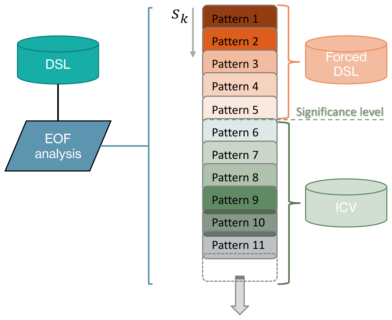
Figure 1Main steps involved in isolating the forced response, including variability decomposition (EOF analysis), finding leading anomaly patterns, and combining leading patterns above a significant statistical level.
To apply S/N M EOF pattern filtering, we must determine two parameters: (1) the number of EOFs retained (N) and (2) the number of S/N patterns used to compose the forced response (M). Following the approach by Wills et al. (2020), we choose N to retain between 75 % and 95 % of the total variance. We use a block bootstrapping approach to determine M, which consists of taking block samples with replacement from the ensemble members to construct a randomized ensemble wherein the forced response timing of their realizations should not agree with one another. Here, we choose 30-year blocks to distinguish forced patterns from ICV so that most of the ICV in DSL is excluded. S/N EOF pattern filtering is then applied to randomized ensembles and the sk value of the pattern with the highest S/N ratio is taken as a threshold. This allows us to obtain a distribution of sk values (one for each randomized ensemble produced) from which a desired confidence level can be estimated. S/N M EOF patterns with a higher sk value than the threshold can be considered part of the forced response with the chosen confidence level (Fig. 1). As there is no sufficient statistical evidence to include patterns with a lower sk value in the forced response, those are considered noise (ICV).
In contrast to S/N M EOF, LFCA identifies the signal that makes it through a low-pass filter. The advantage of LFCA is that it can analyze the forced response in a single ensemble member without relying on the pre-industrial control run (Schneider and Held, 2001; Wills et al., 2018). LFCA is similar to S/N M EOF pattern filtering, but, instead of using an ensemble mean, it detects anomaly patterns associated with time series tk (Eq. 2) that maximize the ratio of low-frequency signal to total variance. The failure to detect some forced variations such as those driven by volcanic activity in surface air temperature and some changes in the seasonal cycle is the main disadvantage of this method being documented in the literature (Wills et al., 2020).
Variations that make it through a low-pass filter (denoted by a tilde) constitute the low-frequency signal (forced response). Here, we apply a linear Lanczos filter (Duchon, 1979) with a 30-year low-pass filter, so only variability at larger timescales is included. Following the same process as in S/N M EOF, a forced response can be constructed by linearly combining leading anomaly patterns, as illustrated in Fig. 1.
3.2 Pattern scaling
Pattern scaling is usually based on grid-point regression against a global variable, and it assumes that a regional change in DSL can be explained by global changes in the predictor(s) of choice. Previous studies have shown that such relationships can be a reasonable approximation for different variables of the climate system. For instance, local surface air temperature change (Collins et al., 2013; Hawkins and Sutton, 2012) and local precipitation (Osborn et al., 2016) have successfully been linked to GSAT change. Regional emulation based on pattern scaling assumes that patterns of local response to external forcing remain constant (Tebaldi and Arblaster, 2014), an assumption that can lead to errors (Wells et al., 2022). However, its simplicity and transferability to many regional variables have made it a popular approach for exploring regional changes in climate change studies (Bilbao et al., 2015; Fox-Kemper, 2021; Herger et al., 2015; Mitchell, 2003; Osborn et al., 2016; Perrette et al., 2013; Tebaldi and Arblaster, 2014; Thomas and Lin, 2018; Wells et al., 2022; Wu et al., 2021; Yuan and Kopp, 2021).
Once we have identified the forced DSL within an ensemble of realizations or a single simulation (as outlined in Sect. 3.1), we will use this forced response as a predictand in our statistical model for projecting regional DSL. There are different forms of pattern scaling, mostly differing in the number of predictors included in the analysis (e.g., univariate, Bilbao et al., 2015; bivariate, Yuan and Kopp, 2021). Here, for simplicity and to ease comparison between raw (dedrifted) DSL and its pattern-filtered equivalent, we only test pattern scaling based on GMTSLR (or zostoga) as a predictor. The univariate case of pattern scaling for relating DSL with GMTSLR can be described by the following linear regression relationship:
where ζ and denote DSL and GMTSLR, respectively. Longitude and latitude are represented by x and y, whereas t denotes time. α is a spatial pattern that captures the scaling relationship between DSL and GMTSLR, and b is an intercept term, both being only a function of location. ε is a residual term regarded as random noise and often assumed to be driven by internally generated variability (Bilbao et al., 2015).
4.1 Forced response in MPI-GE and efficiency of pattern filtering
In this section, we focus on determining the forced response in DSL within a SMILE (MPI-GE) using S/N M EOF pattern filtering and show the efficiency of the latter to remove ICV compared to the more conventional approach of ensemble averaging. To construct the forced response based on S/N patterns, we follow the block bootstrapping approach described in Sect. 3.1. We define blocks in terms of 30 years, so most ICV in DSL is excluded. The 30-year block samples are taken from the 100 historical realizations of the MPI-GE to construct 20 randomized ensembles. A value of 20 is chosen because increasing it further does not lead to substantial changes in the estimation of the 95th percentile of Sk. The estimated ratio Sk (Eq. 1) for a 95 % confidence level is 0.08, leading to a total of eight patterns that can be considered part of the forced response at such a confidence level (Fig. 1).
Even though patterns constructed based on EOFs are created from mathematical constraints, known physical processes can be identified in some patterns. For instance, the S/N M EOF pattern with the highest Sk value, pattern 1 (Fig. 3), explains 62 % of the forced response variance (Fig. 2) and is similar to the main forced pattern of DSL change field driven by increased radiative forcing due to increased GHG emissions. There is a zonal dipole in the Southern Ocean, with decreased and increased sea level relative to the mean below and above 50∘ S, respectively (e.g., Frankcombe et al., 2013). Another dipole structure is found in the North Atlantic with a decreased DSL in the north compared to an increased DSL in the southern section, a feature which appears to disagree with some models (e.g., Bouttes et al., 2014). Nonetheless, the North Atlantic Ocean is an area of large model spread in both CMIP5 and CMIP6 models (Lyu et al., 2020), which suggests that the representation of such a zonal dipole may be model-dependent. Other relevant features include a large DSL rise in the Beaufort Sea and an increased DSL in the northwestern Pacific Ocean. Most of these features agree with those documented among CMIP6 and earlier models (Church et al., 2013; Ferrero et al., 2021; Landerer et al., 2007; Lowe and Gregory, 2006; Lyu et al., 2020; Slangen et al., 2014). Patterns are similar between RCP scenarios, mainly differing in their intensity.
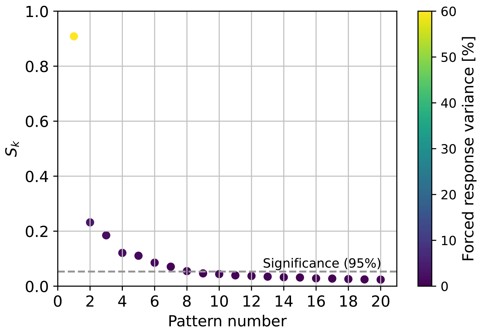
Figure 2Signal fraction of the leading S/N M EOF patterns along with their respective explained forced response variance (%). The significance level (95 %) computed using 30-year block bootstrapping is represented as a dashed line. Patterns are sorted based on the magnitude of their signal fraction, as illustrated in Fig. 1.
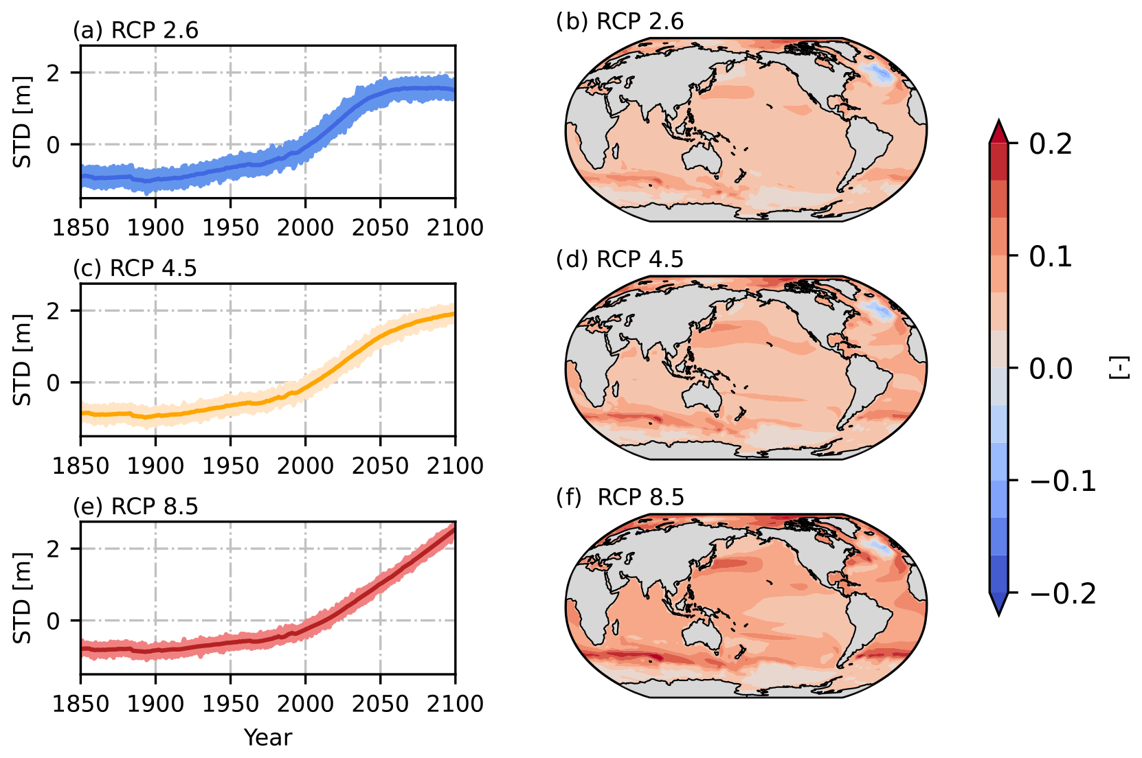
Figure 3Time evolution of DSL standard deviation (a, c, and e) and associated S/N M EOF pattern number 1 for RCP2.6, 4.5, and 8.5 (b, d, and f, respectively). Light colored lines in (a), (c), and (d) represent standard deviation anomalies from ensemble members, whereas dark colored lines depict the ensemble-mean evolution of the pattern. In the historical + RCP scenarios DSL is calculated relative to the mean of 1993–2012.
The three following resulting patterns (patterns 2–4, Figs. S1–S3) represent between 4 % and 1 % (Fig. 2) of the forced response variance and, although with a much lower importance than pattern 1, when combined together represent nonlinear processes that start to have an effect in DSL after 2050. Patterns 5, 6, 7, and 8 (Figs. S4–S7) explain between 1 % and 0.7 % of the forced response variance (Fig. 2) and show a rather stable temporal evolution except for perturbations that coincide with historical volcanic eruptions from Krakatoa, Agung, El Chinchón, and Pinatubo. Volcano-induced perturbations were also observed in the analysis by Wills et al. (2020), as aerosol changes in the atmosphere can affect global and regional temperatures, subsequently affecting DSL. Patterns 9 and beyond explain a variance of less than 0.6 % and since their Sk value is not statistically significant at the 95 % level they could be caused by chance.
We first compare the efficiency of pattern filtering techniques to that of conventional methods, in particular an ensemble mean, to isolate the forced response in DSL. We follow the approach used by Wills et al. (2020) based on the number of ensemble members needed to constrain a certain level of variance of the forced response using the coefficient of determination r2, which indicates the proportion of variance shared between two datasets. As we need two datasets for such a comparison, the 100-member MPI-GE ensemble is divided into two sub-ensembles: one is used for testing (estimate ensemble) and the other is left for reference (reference ensemble). This leaves us with two 50-member sub-ensembles; all 50 members in the reference sub-ensemble are used to estimate the forced response by using either ensemble averaging or S/N M EOF pattern filtering, and this reference sub-ensemble is considered to be ground truth. The other (estimate) 50-member ensemble is also used to estimate the forced response, but instead of using all sub-ensemble members we estimate the forced response in an iterative process by increasing the number of members included in the analysis from 2 to 50. As an illustration of the procedure, we start with only two members, which are used to characterize the forced response in the estimate sub-ensemble, and compare the result with the forced response from the 50-member reference sub-ensemble. This comparison is performed via the coefficient of determination between two estimated forced responses on a grid-point basis, identifying where the 80 % level is exceeded. Grid points where the threshold is not reached are used for subsequent analysis where an additional member (three in total) is included in the estimate sub-ensemble, repeating the same process until the latter reaches 50 members. This procedure enables an evaluation of the number of ensemble members needed in the estimate sub-ensemble to characterize the forced response based on explained variance (i.e., r2) in the reference sub-ensemble. To consider sampling uncertainty, this process is repeated 10 times for random choices of realizations, taking the median value of all iterations.
When simple averaging is used, we find that 50 members are not sufficient to constrain at least 80 % of the forced response variance of the reference ensemble over most of the ocean surface (Fig. 4a). In contrast, S/N M EOF pattern filtering characterizes the forced response more efficiently than simply averaging, as it requires a much smaller number of realizations to remove ICV (Fig. 4b). While the grid-point median value of the number of ensemble members required is 50 or more when using simple averaging, the median estimate for the filtering method is reduced to 8. Large areas of the ocean benefit from filtering, noting significant reductions in the Indian Ocean, South Atlantic, and northeastern Atlantic Ocean, as well as large areas in the Pacific Ocean (Fig. 4b). Other areas, however, remain over the 50-member threshold to explain forced response variance after filtering. Those areas are mostly found where strong western boundary currents exist (Imawaki et al., 2013), as well as in areas influenced by the Antarctic Circumpolar Current (Rintoul et al., 2001). In those locations, variability is higher, and a larger number of realizations is needed to characterize it. Yet, there clearly is an advantage in using S/N M EOF over simple averaging methods, as fewer realizations are required to explain a significant part of the forced response in DSL, which means that the forced response can also be determined in models with smaller ensembles.
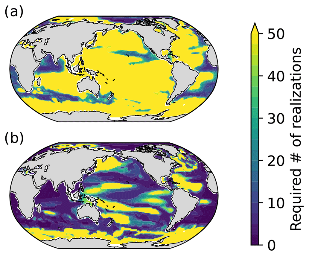
Figure 4The number of ensemble members (realizations) needed to form an MPI-GE sub-ensemble that shares at least 80 % of the variance of the forced response with a reference 50-member MPI-GE sub-ensemble using an ensemble average (a) and using S/N M EOF pattern filtering (b) for RCP2.6. The reference dataset is an average (a) or S/M EOF-filtered sub-ensemble (b) of 50 members which does not share realizations with the sub-ensemble used for estimation. Values represent the median of 10 random choices of realizations sampling for both estimate and reference sub-ensembles. Note that bright yellow indicates that more than 50 ensemble members are required.
4.2 Improved pattern scaling using SMILEs
In this section, we demonstrate how S/N M EOF pattern filtering can increase the capabilities of statistical approaches for explaining DSL based in GMTSLR by reducing ICV within SMILEs. For comparison, we first show pattern scaling performance when using single realizations and how conventional methods (ensemble mean) reduce root mean square error (RMSE) when using a couple of realizations instead. Second, we examine S/N M EOF as a method for reducing RMSE more efficiently. We compare regional RSME from both ensemble mean and pattern filtering on only two realizations to allow an assessment of the areas that benefit the most from filtering when a few simulations are available. Lastly, we contrast how both ensemble mean and S/N M EOF pattern filtering reduce global-mean RMSE as the number of realizations included in the analysis is increased.
As pattern scaling is performed on a grid-point basis, regression performances can be location-dependent (Fig. 5a). Despite such regional variations, we found no substantial differences between GHG scenarios for the regional or global-mean RMSE estimates when pattern-scaling DSL simulations extending up to 2100. Thus, results shown and discussed here are pertinent to the historical + RCP2.6 scenario for illustrative purposes, unless otherwise stated. When applying pattern scaling to a single realization of DSL from MPI-GE, the area-weighted, ensemble average RMSE is 3.78 cm, a value which is similar to previous estimates from studies performed on some of the CMIP5 models (Bilbao et al., 2015; Yuan and Kopp, 2021). However, pattern scaling performance shows a large spatial variability, ranging from 1.13 to 14.95 cm regionally (Fig. 5a). High RMSE values (i.e., lower regression performance) can be found in places subject to nonlinear mesoscale processes driven by strong currents, coinciding with the places where the S/N M EOF technique requires many realizations to explain at least 80 % of the forced response variance (Fig. 4b). These are the Antarctic Circumpolar Current (Southern Ocean) or western boundary currents, including the Gulf Stream (western North Atlantic), Agulhas Current (South Africa), and Kuroshio Current (western North Pacific), as well as at the Brazil–Malvinas Confluence (western South Atlantic). Low RMSE values are found in the more stable eastern boundary currents, such as the Humboldt (Peru) Current, and in equatorial locations where DSL is relatively less influenced by large modes of climate variability (e.g., equatorial Atlantic and Indian Ocean).
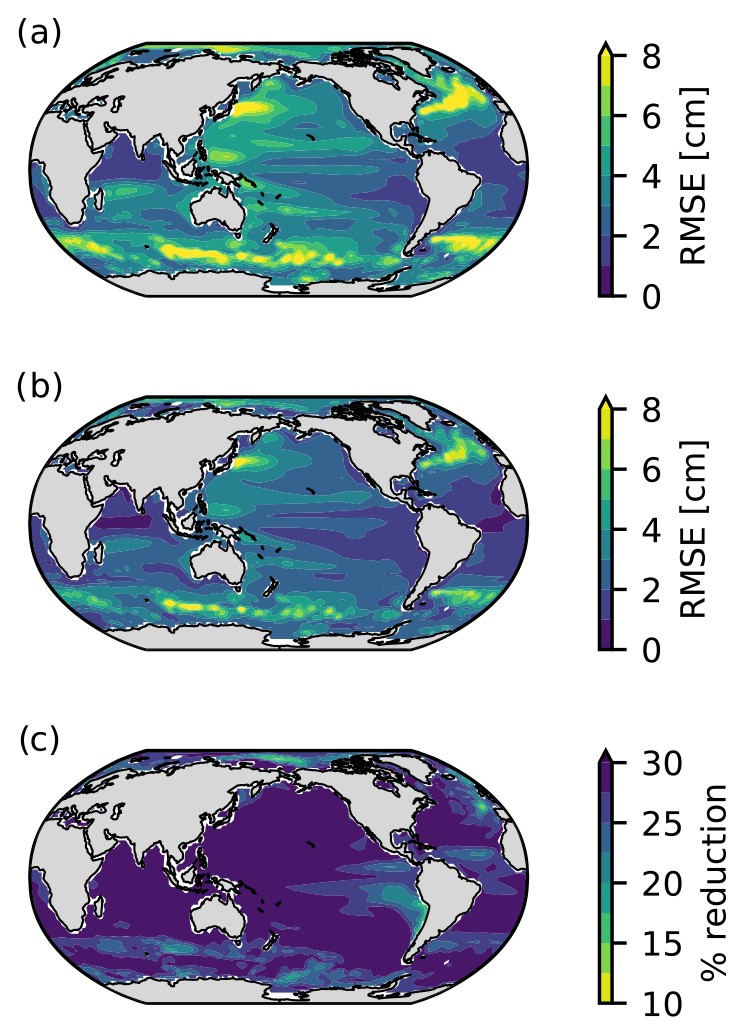
Figure 5Regional pattern scaling performance based on regression RMSE when one realization (a) and a two-member ensemble average (b) are used in the univariate regression. Sampling uncertainty is accounted for in (a) by averaging RMSE from pattern scaling performed individually for the 100 realizations, whereas in (b) random pairs (without replacement) are taken for the two-member ensemble average. The difference in regression performance between (a) and (b) is shown in (c) in terms of percentage. Results are shown for RCP2.6 as an example.
Despite its inefficiency, using an ensemble average cancels out some of the ICV that varies in a different phase between realizations. When using a two-member ensemble mean, RMSE reduction is observed both globally and regionally: the area-weighted average RMSE estimate is reduced from 3.78 to 2.77 cm (27 % reduction) when two ensembles are used, with regional values ranging from 0.87 to 11.00 cm (Fig. 5b). This translates to increased statistical model capabilities within the entire model domain. While grid-point RMSE reduction ranges from 10 % to 30 %, the majority of the ocean benefits from a decrease of more than 25 % due to the removal of some of the ICV (Fig. 5c). Locations experiencing less improvement in regression performance include those that already performed relatively well prior to averaging and those with a high ICV.
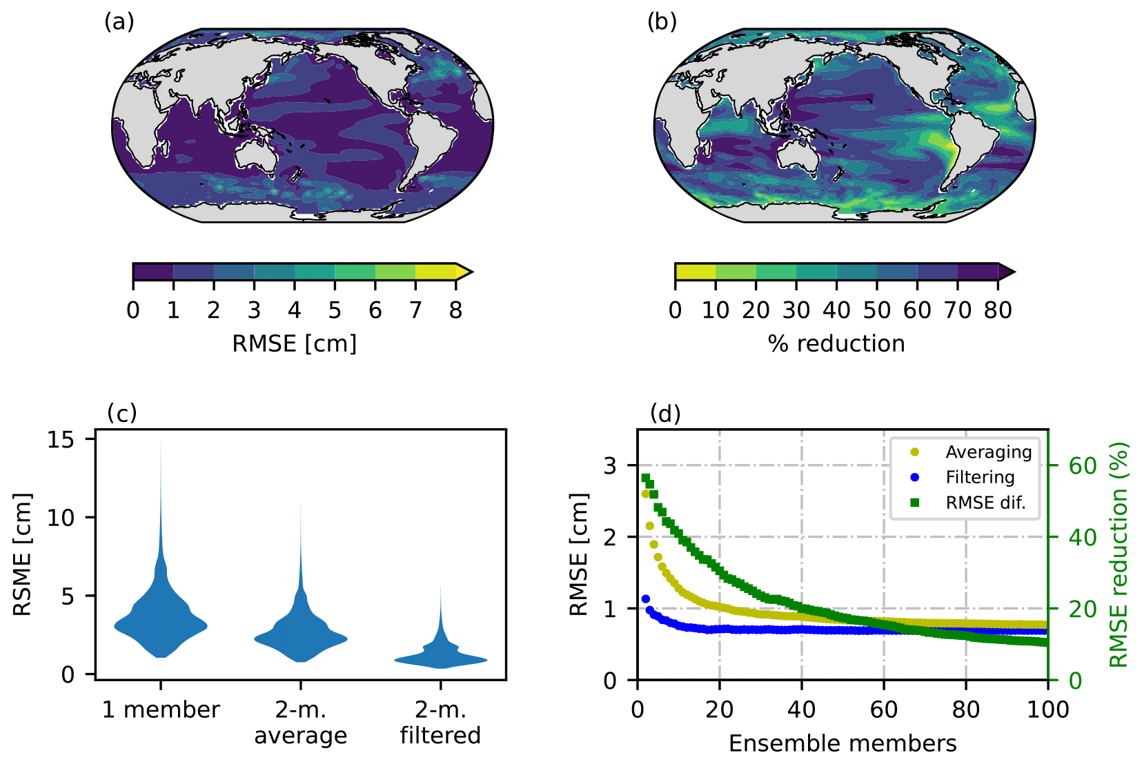
Figure 6Regional pattern scaling performance based on regression RMSE when two ensemble members are used to estimate the forced response via S/N M EOF pattern filtering (a). Panel (b) shows the difference in regression performance between the two-member average pattern scaling (Fig. 5b) and the S/N M EOF-filtered equivalent (a). Panel (c) shows violin plots of RMSE distributions from the one-member, two-member average, and two-member S/N M EOF-filtered approaches. Panel (d) shows the area-weighted average RMSE obtained in the regression as a function of the number of ensemble members included when using an ensemble mean (yellow) and filtering (blue). The difference in performances in terms of percentage is shown in green. The analysis is for the RCP2.6 scenario (we observed no discernible differences between scenarios).
To compare how S/N M EOF pattern filtering improves pattern scaling as opposed to averaging, we take two ensemble members from the MPI-GE historical + RCP2.6 experiment and proceed to remove their ICV by pattern filtering. The two-member pattern-filtered DSL (Fig. 6a) shows an improved RMSE with similar regional structures compared to its averaged counterpart (Fig. 5b), featuring higher values in western boundary currents and the Southern Ocean. Nonetheless, the overall improvement is apparent in all areas: the global estimated RMSE from the regression decreases almost 60 % from an average value of 2.77 to 1.12 cm (Fig. 6c and d). Regionally, RMSE ranges from 0.39 to 6.05 cm when filtering is applied to two ensemble members (Fig. 6a and c). The differences between averaged and filtered approaches are substantial and location-dependent, with filtering yielding a decrease in RMSE ranging from 12 % to about 80 % (Fig. 6b). The tropical Indian and eastern Pacific Ocean are among the locations benefiting the most from the largest performance improvement, which highlights the skill of pattern filtering to remove variability associated with large climate modes (e.g., the El Niño–Southern Oscillation, or ENSO, has a large influence on sea level in the eastern Pacific Ocean). Similar to previous findings when using averaging (Fig. 4c), pattern filtering offers a reduced improvement in areas where regression already performed relatively well or where the presence of mesoscale processes is significant. Regardless of improvement magnitude, pattern filtering provides an overall increase in regression performance that is observable in the entire ocean domain. While averaging also offers an enhancement of pattern scaling skill, filtered two-member pairs produce a distribution of RMSE that is significantly superior (Fig. 6c).
We further investigate how pattern filtering enhances regression compared to averaging by increasing the number of members included in the analysis (Fig. 6d). Increasing the number of realizations grants ensemble averaging a considerable decrease in RSME. Yet, performance improvement asymptotically reaches a plateau around 20 members after which further reductions in RMSE are modest. Regression based on pattern-filtered DSL also shows an improvement as the number of realizations increases. Such improvement is very limited compared to that shown by averaging, although filtering always provides a superior performance regardless of the number of members incorporated in the analysis. Importantly, area-weighted RMSE values differ significantly between the considered approaches when only a small number of realizations are available and become more similar for a larger number. This highlights the role of pattern filtering techniques when only a few ensemble members are available. Based on the analysis performed on the DSL simulations from the MPI-GE, filtering two members provides a regression performance that would only be achieved by averaging at least 12 members.
4.3 Improved pattern scaling using single realizations
Most models in CMIP prior to CMIP6 (and some in CMIP6) provided only one realization of historical and scenario simulations. Therefore, we now test whether pattern filtering could improve regional emulation of single-realization models. To do so, we apply LFCA, which uses an approach similar to S/N M EOF (as explained in Sect. 3.1). In this section, we first examine how LFCA improves the regression RMSE by truncating ICV in a single simulation from the MPI-GE. We then apply LFCA to a range of CMIP5 models that were used in previous patterns scaling analyses of DSL, focusing on the differences between models and RCP scenarios in longer simulations.
LFCA filtering uses the same linear algebra machinery as S/N M EOF, providing a similar regional performance in pattern scaling (compare Fig. 6a and 7a). In some areas, slightly higher RMSE values are observed in LFCA-based regression, for instance in the Southern Ocean. This is expected because only one simulation is used compared to two simulations in S/N M EOF filtering, which enables the latter to identify a larger proportion of ICV. LFCA provides a substantial reduction in RMSE compared to using a single simulation in pattern scaling (Fig. 7b and c). Regionally, it shows a similar qualitative pattern of improvement as the other methods shown here (Fig. 7b vs Figs. 5c and 6b; averaging and S/N M EOF filtering, respectively). Quantitatively, however, LFCA provides a larger global-mean RMSE reduction on a single realization than S/N M EOF performed on two. LFCA provides a reduction of the area-weighted average RMSE of 68 % for all radiative forcing scenarios (Fig. 7c), while S/N M EOF yields 67 % when using two realizations relative to unfiltered one-member pattern scaling. While both estimates are quite similar, it is worth noting that S/N M EOF requires two ensemble members to provide such reduction, while LFCA leads to a similar performance using just one simulation. Similar to S/N M EOF pattern filtering, no substantial differences are found in pattern scaling RMSE between RCP scenarios up to 2100 (Fig. 7c). This implies that ICV is analogous for different RCP scenarios, which, since a reduction in RMSE is due to the removal of ICV, leads to a similar improvement in performance for all RCPs both globally (Fig. 7c) and regionally (not shown).
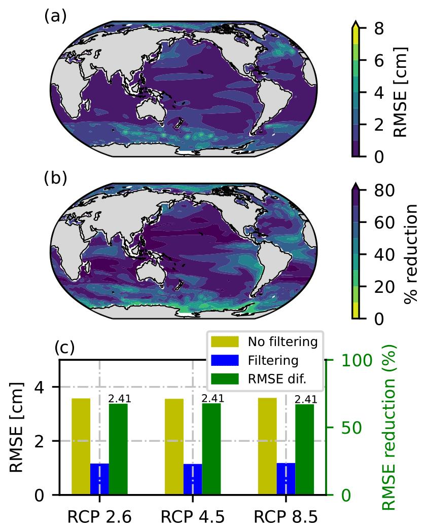
Figure 7Regional pattern scaling performance based on regression RMSE when one (RCP2.6) ensemble member is filtered via LFCA (a). Filtering is performed individually for each ensemble member to compute 100 scaling patterns whose results are averaged to diminish sampling issues. Differences in regression performance between Fig. 5a (unfiltered one-member pattern scaling) and panel (a) are shown in (b) in terms of percentage. The area-weighted average RMSE is shown in (c) for RCP2.6, 4.5, and 8.5 and depending on whether the ensemble member is (blue) or is not (yellow) filtered. Green indicates RMSE reduction between approaches in terms of percentage, whereas values on top of the bars are the absolute differences in centimeters.
Since the aim of this study is to explore differences in emulated DSL when ICV is reduced, we also assess potential differences between unfiltered and filtered simulations (Fig. 8) when predicting DSL at 2100 using GMTSLR as a predictor. Emulated DSL differences caused by filtering may differ depending on the realization used, as each realization features an ICV evolving in a different phase. Thus, we focus on the maximum emulated DSL differences that filtering causes out of all 100 MPI-GE simulations. Exploring the maximal potential difference in statistically projected DSL is an added benefit of using SMILEs, as such an analysis can only be done with a large set of realizations with out-of-phase variability.
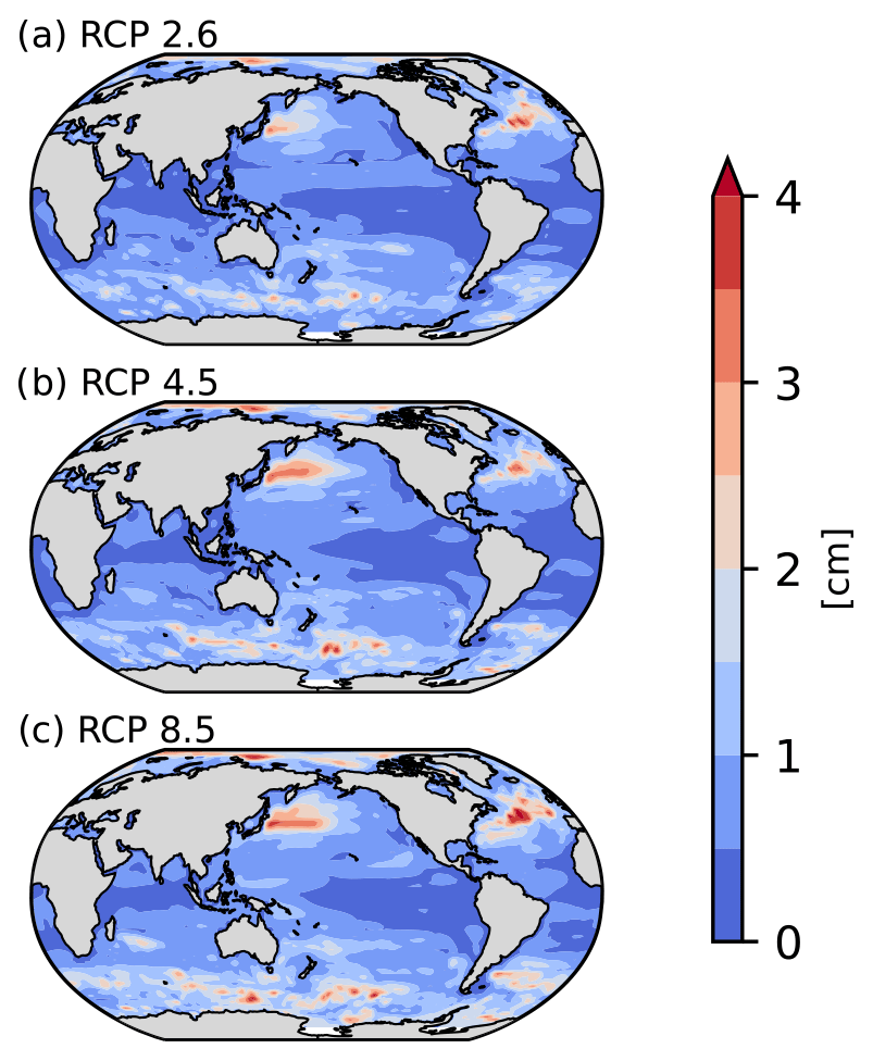
Figure 8Maximum difference between DSL change in 2100 obtained by pattern scaling with coefficients fitted to unfiltered and LFCA-filtered realizations, considering all 100 MPI-GE members, for RCP2.6, RCP4.5, and RCP8.5 (a, b, and c, respectively).
The difference in emulated DSL varies geographically (Fig. 8), with a spatial variability resembling the RMSE when ICV is reduced (e.g., Figs. 6a and 7a). Areas characterized by high temporal variability, which pattern filtering does not completely remove, experience greater difference in DSL projections (Fig. 8). Unlike RMSE (e.g., Fig. 7a), the difference between emulated DSL differs between RCP scenarios, increasing in magnitude with radiative forcing (Fig. 8). RMSE measures the error throughout the entire regression without accounting for the predictor, so only the effect of reduced ICV is captured. On the other hand, an increasing difference in predicted DSL with stronger RCP is expected since the magnitude of the predictor (GMTSLR) is larger for higher emissions scenarios. However, we observe the opposite behavior when assessing the difference in emulated DSL in relative terms, i.e., when the difference is divided by the emulated unfiltered DSL or by GMTSLR in 2100 (not shown). Despite contrast between RCPs either in total difference (slightly increasing with forcing) or relative terms (decreasing with increasing forcing), RMSE being similar between RCPs highlights the fact that pattern filtering may be relevant for all scenarios.
The effect of pattern filtering on differences in slope α, a key parameter in pattern scaling, again shows spatial variability similar to RMSE (Fig. 7 vs Fig. S8). Changes in slopes are substantial in places with high variability, sometimes even showing a sign change (e.g., Fig. S13). Contrary to the total difference in emulated DSL and similar to the relative one, slope differences tend to decrease with higher emissions scenarios (Fig. S8). Since lower radiative forcing means lower signal-to-noise ratio, noise (ICV) can drive large differences in slopes between filtered and unfiltered results, and vice versa. Apart from reducing RMSE and leading to narrower confidence intervals (e.g., Figs. S10–S14), pattern filtering finds slopes that are significantly different from that obtained by applying a moving mean (e.g., Figs. S12 and S14), as the latter does not remove ICV as efficiently and requires neglecting data points for its computation (Figs. S10b–S14b). It is worth highlighting that these differences in emulated DSL and slopes showcase an example for a GCM and may not hold as ground truth for other GCMs, scenarios, or predictors used.

Figure 9Area-weighted average RMSE for RCP2.6, 4.5, and 8.5, indicating whether the ensemble member is (blue) or is not (yellow) filtered via LFCA. Green indicates relative RMSE reduction between approaches (%), whereas values on top of the bars are the absolute differences in centimeters. Different panels represent different CMIP5 models. The main panel includes simulation data up to 2300, whereas the small inset in the right-hand top corner shows RMSE results up to 2100. Small insets share the same axes as main panels.
We further explore the performance of LFCA by comparing the pattern scaling results when isolating the forced response for other GCMs. We identify the forced DSL in four CMIP5 models: GISS-E2-R, HadGEM2-ES, IPSL-CM5A-LR, and MPI-ESM-LR (Fig. 9a–d, respectively), which all provide scenario simulations up to 2300. To ease comparison with results from the MPI-GE, however, we first examine results up to 2100 (Fig. 9a–d, small right-hand-side insets). RMSEs from unfiltered simulations up to 2100 vary between models, and so does RMSE reduction provided by LFCA. Nonetheless, error reduction within a model and between scenarios is very similar, as previously observed for the MPI-GE. This implies that, for all models considered here, there are no significant changing behaviors in the relationship between DSL and GMTLSR between RCP scenarios up to 2100.
When considering results up to 2300, pattern scaling of unfiltered DSL against GMTSLR yields similar results as previous studies (Bilbao et al., 2015), showing a global area-weighted mean RMSE between 2 and 4 cm. RMSE in both unfiltered and filtered simulations of DSL increases with radiative forcing for all models considered. As simulations run up to 2300, a decrease in pattern scaling performance for higher RCPs may indicate a more important role of the deeper ocean layer driving nonlinear processes (Bilbao et al., 2015; Yuan and Kopp, 2021). This tendency is also reflected in the error reduction after filtering, which decreases as radiative forcing increases both over time and because of the higher emissions scenario, but the latter is more apparent. Although LFCA filtering improves the performance of pattern scaling for all four CMIP5 models, considerable differences in error reductions are observed. For instance, HadGEM2-ES benefits the most from pattern filtering between all the models, with a ∼ 70 % decrease in error for RCP2.6. Conversely, GISS-E2-R undergoes the lowest reduction after pattern filtering, with about a 50 % increase in performance for the same RCP scenario. Differences in model performance pre- and post-filtering not only highlight differences in how ICV is represented in distinct models but may also reflect model differences in terms of physics representation and modeled forced response.
Regional emulation tools for DSL change are complementary approaches to GCMs that allow for computationally cheap statistical projections. Most DSL regional emulators are based on pattern scaling, a statistical model usually based on a grid-point regression against a global variable representing change in the climate system driven by external forcing. While choosing suitable global predictors is essential for appropriate tuning of the statistical model, random errors can remain, leading to high uncertainties in statistically based projections. Some of these random errors are driven by ICV in DSL and can be characterized using macro-initialized initial-condition large ensembles (SMILEs), which are designed to facilitate a separation between ICV and external forcings within a model. Here, we applied pattern recognition techniques to a SMILE with the aim of efficiently truncating ICV, demonstrating how these approaches could significantly reduce random errors in regional emulators of DSL and provide substantially different emulated results in areas with high ICV.
Although ICV can also be reduced by using more conventional methods, such as computing an ensemble mean or linear trends, this requires a relatively large number of realizations to be effective. This is a significant constraint, particularly for modeling experiments featuring a limited number of realizations. A more efficient alternative consists of employing methods that exploit spatial covariance information, such as S/N M EOF pattern filtering and LFCA. We have demonstrated that S/N M EOF applied to two realizations attains the same level of error reduction as averaging 12 realizations. The largest improvement relative to unfiltered simulations was observed when only a few simulations were available, whereas both S/N-filtered and ensemble average model performance tended to converge for a large number of ensemble members. By identifying spatiotemporal coherent structures, the S/N M EOF filtering was particularly skillful at removing ICV due to large modes of climate variability, such as the ENSO influence on sea level in the eastern Pacific.
S/N M EOF pattern filtering can identify the common response within at least two realizations. This motivated us to also test LFCA, which can remove variability in single-realization modeling experiments by applying a low-pass filter. Apart from being computationally more efficient, LFCA outperforms S/N M EOF in improving the performance of DSL pattern scaling when using one or two realizations. Moreover, LFCA applied to individual SMILE realizations allows exploring the maximal potential difference between statistically projected unfiltered and filtered DSL. We found substantial differences in emulated DSL and regression slopes in places with high variability, highlighting the relevance of pattern filtering methods in areas subject to non-mesoscale processes. Despite LFCA versatility and performances results, previous studies have emphasized that S/N M EOF pattern filtering provides a range of benefits compared to LFCA, including (1) a better isolation of the forced response when the number of ensemble members is large and (2) the detection of relatively less important forced patterns, such as those driven by volcanism.
We have also investigated LFCA by applying it to longer (up to 2300) CMIP5 simulations. We found that pattern scaling performance is independent of the GHG emission scenario up to 2100 and decreases with radiative forcing beyond 2100. Since we used a linear model, this implies that nonlinear processes have different effects on DSL depending on the GHG scenario, and this is reflected in a decrease in model performance depending on the emissions. We also found substantial differences between CMIP5 models due to variability being represented differently as well as distinct model physics. Nonetheless, the performance improvement of pattern scaling when applying LFCA filtering is considerable for all models and scenarios, ranging from 20 % to more than 70 % reduction relative to the unfiltered results.
Here, we have demonstrated that reducing ICV increases the capabilities of statistical approaches to project DSL. Pattern recognition techniques are especially advantageous for such a task, as they do not require numerous realizations to significantly reduce uncertainties in statistical projections and no data are lost (as in 30-year means) when reducing ICV. Previous studies have not considered removing ICV, which could significantly reduce uncertainties in statistically projected DSL and lead to substantial differences in emulated DSL. Although the difference in emulated DSL and regression slope varies depending on scenario and results shown here are an example and may differ depending on GCM, RCPs, and predictor used, we show that pattern filtering is a useful approach to consider as a means of enhancing emulated DSL simulations.
Simulations from the MPI-GE can be obtained at https://esgf-data.dkrz.de/projects/mpi-ge/ (ESGF, 2023), whereas CMIP5 data can be found at https://esgf-node.llnl.gov/search/cmip5/ (CMIP5, 2023).
The supplement related to this article is available online at: https://doi.org/10.5194/os-19-499-2023-supplement.
VMS devised, designed, and performed the analysis and wrote the paper. ABAS supervised the study and contributed to writing. THJH contributed to data pre-processing and paper writing. SD and MM provided valuable feedback on methods and contributed to writing. NM provided MPI-GE data and information on MPI-GE methods and contributed to writing.
The contact author has declared that none of the authors has any competing interests.
Publisher's note: Copernicus Publications remains neutral with regard to jurisdictional claims in published maps and institutional affiliations.
Víctor Malagón-Santos, Aimée B. A. Slangen, and Tim H. J. Hermans were supported by PROTECT (see Financial support statement). Sönke Dangendorf acknowledges David and Jane Flowerree for their support. We acknowledge the World Climate Research Programme's Working Group on Coupled Modelling, which is responsible for CMIP, and we thank the climate modeling groups for producing and making available their model output. For CMIP the US Department of Energy's Program for Climate Model Diagnosis and Intercomparison provides coordinating support and led development of software infrastructure in partnership with the Global Organization for Earth System Science Portals.
This publication was supported by PROTECT. This project has received funding from the European Union's Horizon 2020 research and innovation program (grant no. 869304, PROTECT contribution number 61).
This paper was edited by Anne Marie Treguier and reviewed by Kewei Lyu and one anonymous referee.
Becker, M., Karpytchev, M., and Lennartz-Sassinek, S.: Long-term sea level trends: Natural or anthropogenic?, Geophys. Res. Lett., 41, 5571–5580, https://doi.org/10.1002/2014GL061027, 2014.
Bilbao, R. A. F., Gregory, J. M., and Bouttes, N.: Analysis of the regional pattern of sea level change due to ocean dynamics and density change for 1993–2099 in observations and CMIP5 AOGCMs, Clim. Dynam., 45, 2647–2666, https://doi.org/10.1007/s00382-015-2499-z, 2015.
Bouttes, N., Gregory, J. M., Kuhlbrodt, T., and Smith, R. S.: The drivers of projected North Atlantic sea level change, Clim. Dynam., 43, 1531–1544, https://doi.org/10.1007/s00382-013-1973-8, 2014.
Church, J. A., Clark, P. U., Cazenave, A., Gregory, J. M., Jevrejeva, S., Levermann, A., Merrifield, M. A., Milne, G. A., Nerem, R. S., Nunn, P. D., Payne, A. J., Pfeffer, W. T., Stammer, D., and Unnikrishnan, A. S.: Sea Level Change, in: Climate Change 2013: The Physical Science Basis. Contribution of Working Group I to the Fifth Assessment Report of the Intergovernmental Panel on Climate Change, edited by: Stocker, T. F., Qin, D., Plattner, G.-K., Tignor, M., Allen, S. K., Boschung, J., Nauels, A., Xia, Y., Bex, V., and Midgley, P. M., Cambridge University Press, Cambridge, United Kingdom and New York, NY, USA, 2013.
CMIP5: CMIP5 data search, ESGF-cog – Lawrence Livermore National [data set], https://esgf-node.llnl.gov/search/cmip5/, last access: 18 April 2023.
Collins, M., Knutti, R., Arblaster, J., Dufresne, J.-L., Fichefet, T., Friedlingstein, P., Gao, X., Gutowski, W. J., Johns, T., Krinner, G., Shongwe, M., Tebaldi, C., Weaver, A. J., and Wehner, M.: Long-term Climate Change: Projections, Commitments and Irreversibility, in: Climate Change 2013: The Physical Science Basis. Contribution of Working Group I to the Fifth Assessment Report of the Intergovernmental Panel on Climate Change, edited by: Stocker, T. F., Qin, D., Plattner, G.-K., Tignor, M., Allen, S. K., Boschung, J., Nauels, A., Xia, Y., Bex, V., and Midgley, P. M., Cambridge University Press, Cambridge, United Kingdom and New York, NY, USA, 2013.
Cooley, S., Schoeman, D., Bopp, L., Boyd, P., Donner, S., Ghebrehiwet, D. Y., Ito, S.-I., Kiessling, W., Martinetto, P., Ojea, E., Racault, M.-F., Rost, B., and Skern-Mauritzen, M.: Oceans and Coastal Ecosystems and Their Services, in: Climate Change 2022: Impacts, Adaptation and Vulnerability. Contribution of Working Group II to the Sixth Assessment Report of the Intergovernmental Panel on Climate Change, edited by: Pörtner, H.-O., Roberts, D. C., Tignor, M., Poloczanska, E. S., Mintenbeck, K., Alegría, A., Craig, M., Langsdorf, S., Löschke, S., Möller, V., Okem, A., and Rama, B., Cambridge University Press, Cambridge, UK and New York, NY, USA, 379–550, 2022.
Couldrey, M. P., Gregory, J. M., Boeira Dias, F., Dobrohotoff, P., Domingues, C. M., Garuba, O., Griffies, S. M., Haak, H., Hu, A., Ishii, M., Jungclaus, J., Köhl, A., Marsland, S. J., Ojha, S., Saenko, O. A., Savita, A., Shao, A., Stammer, D., Suzuki, T., Todd, A., and Zanna, L.: What causes the spread of model projections of ocean dynamic sea-level change in response to greenhouse gas forcing?, Clim. Dynam., 56, 155–187, https://doi.org/10.1007/s00382-020-05471-4, 2021.
Danabasoglu, G., Lamarque, J.-F., Bacmeister, J., Bailey, D. A., DuVivier, A. K., Edwards, J., Emmons, L. K., Fasullo, J., Garcia, R., and Gettelman, A.: The community earth system model version 2 (CESM2), J. Adv. Model. Earth Sy., 12, e2019MS001916, https://doi.org/10.1029/2019MS001916, 2020.
Dangendorf, S., Rybski, D., Mudersbach, C., Müller, A., Kaufmann, E., Zorita, E., and Jensen, J.: Evidence for long-term memory in sea level, Geophys. Res. Lett., 41, 5530–5537, https://doi.org/10.1002/2014GL060538, 2014.
Dangendorf, S., Hay, C., Calafat, F. M., Marcos, M., Piecuch, C. G., Berk, K., and Jensen, J.: Persistent acceleration in global sea-level rise since the 1960s, Nat. Clim. Change, 9, 705–710, https://doi.org/10.1038/s41558-019-0531-8, 2019.
DelSole, T., Tippett, M. K., and Shukla, J.: A significant component of unforced multidecadal variability in the recent acceleration of global warming, J. Climate, 24, 909–926, 2011.
Deser, C., Lehner, F., Rodgers, K. B., Ault, T., Delworth, T. L., DiNezio, P. N., Fiore, A., Frankignoul, C., Fyfe, J. C., Horton, D. E., Kay, J. E., Knutti, R., Lovenduski, N. S., Marotzke, J., McKinnon, K. A., Minobe, S., Randerson, J., Screen, J. A., Simpson, I. R., and Ting, M.: Insights from Earth system model initial-condition large ensembles and future prospects, Nat. Clim. Change, 10, 277–286, https://doi.org/10.1038/s41558-020-0731-2, 2020.
Duchon, C. E.: Lanczos Filtering in One and Two Dimensions, J. Appl. Meteorol. Clim., 18, 1016–1022, https://doi.org/10.1175/1520-0450(1979)018<1016:LFIOAT>2.0.CO;2, 1979.
Durand, G., van den Broeke, M. R., Le Cozannet, G., Edwards, T. L., Holland, P. R., Jourdain, N. C., Marzeion, B., Mottram, R., Nicholls, R. J., Pattyn, F., Paul, F., Slangen, A. B. A., Winkelmann, R., Burgard, C., van Calcar, C. J., Barré, J.-B., Bataille, A., and Chapuis, A.: Sea-Level Rise: From Global Perspectives to Local Services, Frontiers in Marine Science, 8, https://doi.org/10.3389/fmars.2021.709595, 2022.
Edwards, T. L., Nowicki, S., Marzeion, B., Hock, R., Goelzer, H., Seroussi, H., Jourdain, N. C., Slater, D. A., Turner, F. E., Smith, C. J., McKenna, C. M., Simon, E., Abe-Ouchi, A., Gregory, J. M., Larour, E., Lipscomb, W. H., Payne, A. J., Shepherd, A., Agosta, C., Alexander, P., Albrecht, T., Anderson, B., Asay-Davis, X., Aschwanden, A., Barthel, A., Bliss, A., Calov, R., Chambers, C., Champollion, N., Choi, Y., Cullather, R., Cuzzone, J., Dumas, C., Felikson, D., Fettweis, X., Fujita, K., Galton-Fenzi, B. K., Gladstone, R., Golledge, N. R., Greve, R., Hattermann, T., Hoffman, M. J., Humbert, A., Huss, M., Huybrechts, P., Immerzeel, W., Kleiner, T., Kraaijenbrink, P., Le Clec'h, S., Lee, V., Leguy, G. R., Little, C. M., Lowry, D. P., Malles, J.-H., Martin, D. F., Maussion, F., Morlighem, M., O'Neill, J. F., Nias, I., Pattyn, F., Pelle, T., Price, S. F., Quiquet, A., Radić, V., Reese, R., Rounce, D. R., Rückamp, M., Sakai, A., Shafer, C., Schlegel, N.-J., Shannon, S., Smith, R. S., Straneo, F., Sun, S., Tarasov, L., Trusel, L. D., Van Breedam, J., van de Wal, R., van den Broeke, M., Winkelmann, R., Zekollari, H., Zhao, C., Zhang, T., and Zwinger, T.: Projected land ice contributions to twenty-first-century sea level rise, Nature, 593, 74–82, https://doi.org/10.1038/s41586-021-03302-y, 2021.
Eyring, V., Bony, S., Meehl, G. A., Senior, C. A., Stevens, B., Stouffer, R. J., and Taylor, K. E.: Overview of the Coupled Model Intercomparison Project Phase 6 (CMIP6) experimental design and organization, Geosci. Model Dev., 9, 1937–1958, https://doi.org/10.5194/gmd-9-1937-2016, 2016.
Farrell, W. E. and Clark, J. A.: On postglacial sea level, Geophys. J. Int., 46, 647–667, 1976.
Fasullo, J. T., Gent, P. R., and Nerem, R. S.: Forced Patterns of Sea Level Rise in the Community Earth System Model Large Ensemble From 1920 to 2100, J. Geophys. Res.-Oceans, 125, e2019JC016030, https://doi.org/10.1029/2019JC016030, 2020.
Ferrero, B., Tonelli, M., Marcello, F., and Wainer, I.: Long-term Regional Dynamic Sea Level Changes from CMIP6 Projections, Adv. Atmos. Sci., 38, 157–167, https://doi.org/10.1007/s00376-020-0178-4, 2021.
Fox-Kemper, B., Hewitt, H. T., Xiao, C., A.algeirsd.ttir, G., Drijfhout, S. S., Edwards, T. L., Golledge, N. R., Hemer, M., Kopp, R. E., Krinner, G., Mix, A., Notz, D., Nowicki, S., Nurhati, I. S., Ruiz, L., Sallée, J.-B., Slangen, A. B. A., and Yu, Y.: Ocean, Cryosphere and Sea Level Change, in: Climate Change 2021: The Physical Science Basis. Contribution of Working Group I to the Sixth Assessment Report of the Intergovernmental Panel on Climate Change, edited by: Masson-Delmotte, V., Zhai, P., Pirani, A., Connors, S. L., Péan, C., Berger, S., Caud, N., Chen, Y., Goldfarb, L., Gomis, M. I., Huang, M., Leitzell, K., Lonnoy, E., Matthews, J. B. R., Maycock, T. K., Waterfield, T., Yelekçi, O., Yu, R., and Zhou, B., Cambridge University Press, Cambridge, United Kingdom and New York, NY, USA, 1211–1362, 2021.
Frankcombe, L. M., Spence, P., Hogg, A. M., England, M. H., and Griffies, S. M.: Sea level changes forced by Southern Ocean winds, Geophys. Res. Lett., 40, 5710–5715, 2013.
Frankcombe, L. M., England, M. H., Mann, M. E., and Steinman, B. A.: Separating Internal Variability from the Externally Forced Climate Response, J. Climate, 28, 8184–8202, https://doi.org/10.1175/JCLI-D-15-0069.1, 2015.
Frederikse, T., Landerer, F., Caron, L., Adhikari, S., Parkes, D., Humphrey, V. W., Dangendorf, S., Hogarth, P., Zanna, L., and Cheng, L.: The causes of sea-level rise since 1900, Nature, 584, 393–397, 2020.
Geoffroy, O., Saint-Martin, D., Olivié, D. J., Voldoire, A., Bellon, G., and Tytéca, S.: Transient climate response in a two-layer energy-balance model. Part I: Analytical solution and parameter calibration using CMIP5 AOGCM experiments, J. Climate, 26, 1841–1857, 2013a.
Geoffroy, O., Saint-Martin, D., Bellon, G., Voldoire, A., Olivié, D. J. L., and Tytéca, S.: Transient climate response in a two-layer energy-balance model. Part II: Representation of the efficacy of deep-ocean heat uptake and validation for CMIP5 AOGCMs, J. Climate, 26, 1859–1876, 2013b.
Goodwin, P., Katavouta, A., Roussenov, V. M., Foster, G. L., Rohling, E. J., and Williams, R. G.: Pathways to 1.5 ∘C and 2 ∘C warming based on observational and geological constraints, Nat. Geosci., 11, 102–107, 2018.
Gregory, J. M., Griffies, S. M., Hughes, C. W., Lowe, J. A., Church, J. A., Fukimori, I., Gomez, N., Kopp, R. E., Landerer, F., Cozannet, G. L., Ponte, R. M., Stammer, D., Tamisiea, M. E., and van de Wal, R. S. W.: Concepts and Terminology for Sea Level: Mean, Variability and Change, Both Local and Global, Surv. Geophys., 40, 1251–1289, https://doi.org/10.1007/s10712-019-09525-z, 2019.
Griffies, S. M., Danabasoglu, G., Durack, P. J., Adcroft, A. J., Balaji, V., Böning, C. W., Chassignet, E. P., Curchitser, E., Deshayes, J., Drange, H., Fox-Kemper, B., Gleckler, P. J., Gregory, J. M., Haak, H., Hallberg, R. W., Heimbach, P., Hewitt, H. T., Holland, D. M., Ilyina, T., Jungclaus, J. H., Komuro, Y., Krasting, J. P., Large, W. G., Marsland, S. J., Masina, S., McDougall, T. J., Nurser, A. J. G., Orr, J. C., Pirani, A., Qiao, F., Stouffer, R. J., Taylor, K. E., Treguier, A. M., Tsujino, H., Uotila, P., Valdivieso, M., Wang, Q., Winton, M., and Yeager, S. G.: OMIP contribution to CMIP6: experimental and diagnostic protocol for the physical component of the Ocean Model Intercomparison Project, Geosci. Model Dev., 9, 3231–3296, https://doi.org/10.5194/gmd-9-3231-2016, 2016.
Gupta, A. S., Jourdain, N. C., Brown, J. N., and Monselesan, D.: Climate drift in the CMIP5 models, J. Climate, 26, 8597–8615, 2013.
Haasnoot, M., Brown, S., Scussolini, P., Jimenez, J. A., Vafeidis, A. T., and Nicholls, R. J.: Generic adaptation pathways for coastal archetypes under uncertain sea-level rise, Environ. Res. Commun., 1, 071006, https://doi.org/10.1088/2515-7620/ab1871, 2019.
Haasnoot, M., Winter, G., Brown, S., Dawson, R. J., Ward, P. J., and Eilander, D.: Long-term sea-level rise necessitates a commitment to adaptation: A first order assessment, Climate Risk Management, 34, 100355, https://doi.org/10.1016/j.crm.2021.100355, 2021.
Haigh, I. D., Pickering, M. D., Green, J. A. M., Arbic, B. K., Arns, A., Dangendorf, S., Hill, D. F., Horsburgh, K., Howard, T., Idier, D., Jay, D. A., Jänicke, L., Lee, S. B., Müller, M., Schindelegger, M., Talke, S. A., Wilmes, S.-B., and Woodworth, P. L.: The Tides They Are A-Changin': A Comprehensive Review of Past and Future Nonastronomical Changes in Tides, Their Driving Mechanisms, and Future Implications, Rev. Geophys., 58, e2018RG000636, https://doi.org/10.1029/2018RG000636, 2020.
Hasselmann, K.: Stochastic climate models part I. Theory, Tellus, 28, 473–485, 1976.
Hawkins, E. and Sutton, R.: Time of emergence of climate signals, Geophys. Res. Lett., 39, https://doi.org/10.1029/2011GL050087, 2012.
Hawkins, E., Smith, R. S., Gregory, J. M., and Stainforth, D. A.: Irreducible uncertainty in near-term climate projections, Clim. Dynam., 46, 3807–3819, https://doi.org/10.1007/s00382-015-2806-8, 2016.
Herger, N., Sanderson, B. M., and Knutti, R.: Improved pattern scaling approaches for the use in climate impact studies, Geophys. Res. Lett., 42, 3486–3494, https://doi.org/10.1002/2015GL063569, 2015.
Hermans, T. H. J., Tinker, J., Palmer, M. D., Katsman, C. A., Vermeersen, B. L. A., and Slangen, A. B. A.: Improving sea-level projections on the Northwestern European shelf using dynamical downscaling, Clim. Dynam., 54, 1987–2011, https://doi.org/10.1007/s00382-019-05104-5, 2020.
Hinkel, J., Lincke, D., Vafeidis, A. T., Perrette, M., Nicholls, R. J., Tol, R. S., Marzeion, B., Fettweis, X., Ionescu, C., and Levermann, A.: Coastal flood damage and adaptation costs under 21st century sea-level rise, P. Natl. Acad. Sci. USA, 111, 3292–3297, 2014.
Hobbs, W., Palmer, M. D., and Monselesan, D.: An energy conservation analysis of ocean drift in the CMIP5 global coupled models, J. Climate, 29, 1639–1653, 2016.
Imawaki, S., Bower, A. S., Beal, L., and Qiu, B.: Chapter 13 – Western Boundary Currents, in: International Geophysics, vol. 103, edited by: Siedler, G., Griffies, S. M., Gould, J., and Church, J. A., Academic Press, 305–338, https://doi.org/10.1016/B978-0-12-391851-2.00013-1, 2013.
Kay, J. E., Deser, C., Phillips, A., Mai, A., Hannay, C., Strand, G., Arblaster, J. M., Bates, S. C., Danabasoglu, G., and Edwards, J.: The Community Earth System Model (CESM) large ensemble project: A community resource for studying climate change in the presence of internal climate variability, B. Am. Meteorol. Soc., 96, 1333–1349, 2015.
Labe, Z. M. and Barnes, E. A.: Detecting Climate Signals Using Explainable AI With Single-Forcing Large Ensembles, J. Adv. Model. Earth Sy., 13, e2021MS002464, https://doi.org/10.1029/2021MS002464, 2021.
Landerer, F. W., Jungclaus, J. H., and Marotzke, J.: Regional dynamic and steric sea level change in response to the IPCC-A1B scenario, J. Phys. Oceanogr., 37, 296–312, 2007.
Lowe, J. A. and Gregory, J. M.: Understanding projections of sea level rise in a Hadley Centre coupled climate model, J. Geophys. Res.-Oceans, 111, C11014, https://doi.org/10.1029/2005JC003421, 2006.
Lyu, K., Zhang, X., and Church, J. A.: Regional Dynamic Sea Level Simulated in the CMIP5 and CMIP6 Models: Mean Biases, Future Projections, and Their Linkages, J. Climate, 33, 6377–6398, https://doi.org/10.1175/JCLI-D-19-1029.1, 2020.
Maher, N., Milinski, S., Suarez-Gutierrez, L., Botzet, M., Dobrynin, M., Kornblueh, L., Kröger, J., Takano, Y., Ghosh, R., Hedemann, C., Li, C., Li, H., Manzini, E., Notz, D., Putrasahan, D., Boysen, L., Claussen, M., Ilyina, T., Olonscheck, D., Raddatz, T., Stevens, B., and Marotzke, J.: The Max Planck Institute Grand Ensemble: Enabling the Exploration of Climate System Variability, J. Adv. Model. Earth Sy., 11, 2050–2069, https://doi.org/10.1029/2019MS001639, 2019.
Maher, N., Milinski, S., and Ludwig, R.: Large ensemble climate model simulations: introduction, overview, and future prospects for utilising multiple types of large ensemble, Earth Syst. Dynam., 12, 401–418, https://doi.org/10.5194/esd-12-401-2021, 2021a.
Maher, N., Power, S., and Marotzke, J.: More accurate quantification of model-to-model agreement in externally forced climatic responses over the coming century, Nat. Commun., 12, 788, https://doi.org/10.1038/s41467-020-20635-w, 2021b.
Mankin, J. S., Lehner, F., Coats, S., and McKinnon, K. A.: The Value of Initial Condition Large Ensembles to Robust Adaptation Decision-Making, Earths Future, 8, e2012EF001610, https://doi.org/10.1029/2020EF001610, 2020.
Marcos, M. and Amores, A.: Quantifying anthropogenic and natural contributions to thermosteric sea level rise, Geophys. Res. Lett., 41, 2502–2507, https://doi.org/10.1002/2014GL059766, 2014.
Meinshausen, M., Raper, S. C. B., and Wigley, T. M. L.: Emulating coupled atmosphere-ocean and carbon cycle models with a simpler model, MAGICC6 – Part 1: Model description and calibration, Atmos. Chem. Phys., 11, 1417–1456, https://doi.org/10.5194/acp-11-1417-2011, 2011.
Millar, R. J., Nicholls, Z. R., Friedlingstein, P., and Allen, M. R.: A modified impulse-response representation of the global near-surface air temperature and atmospheric concentration response to carbon dioxide emissions, Atmos. Chem. Phys., 17, 7213–7228, https://doi.org/10.5194/acp-17-7213-2017, 2017.
Mitchell, T. D.: Pattern Scaling: An Examination of the Accuracy of the Technique for Describing Future Climates, Climatic Change, 60, 217–242, https://doi.org/10.1023/A:1026035305597, 2003.
Mitrovica, J. X., Tamisiea, M. E., Davis, J. L., and Milne, G. A.: Recent mass balance of polar ice sheets inferred from patterns of global sea-level change, Nature, 409, 1026–1029, 2001.
Moftakhari, H. R., AghaKouchak, A., Sanders, B. F., Feldman, D. L., Sweet, W., Matthew, R. A., and Luke, A.: Increased nuisance flooding along the coasts of the United States due to sea level rise: Past and future, Geophys. Res. Lett., 42, 9846–9852, 2015.
ESGF: MPI Grand Ensemble – ESGF [data set], https://esgf-data.dkrz.de/projects/mpi-ge/, last access: 18 April 2023.
Nerem, R. S., Leuliette, É., and Cazenave, A.: Present-day sea-level change: A review, C. R. Geosci., 338, 1077–1083, https://doi.org/10.1016/j.crte.2006.09.001, 2006.
Nicholls, R. J., Lincke, D., Hinkel, J., Brown, S., Vafeidis, A. T., Meyssignac, B., Hanson, S. E., Merkens, J.-L., and Fang, J.: A global analysis of subsidence, relative sea-level change and coastal flood exposure, Nat. Clim. Change, 11, 338–342, https://doi.org/10.1038/s41558-021-00993-z, 2021.
O'Neill, B. C., Kriegler, E., Ebi, K. L., Kemp-Benedict, E., Riahi, K., Rothman, D. S., van Ruijven, B. J., van Vuuren, D. P., Birkmann, J., Kok, K., Levy, M., and Solecki, W.: The roads ahead: Narratives for shared socioeconomic pathways describing world futures in the 21st century, Global Environ. Chang., 42, 169–180, https://doi.org/10.1016/j.gloenvcha.2015.01.004, 2017.
Osborn, T. J., Wallace, C. J., Harris, I. C., and Melvin, T. M.: Pattern scaling using ClimGen: monthly-resolution future climate scenarios including changes in the variability of precipitation, Climatic Change, 134, 353–369, https://doi.org/10.1007/s10584-015-1509-9, 2016.
Peltier, W. R.: Global sea level rise and glacial isostatic adjustment, Global Planet. Change, 20, 93–123, 1999.
Peltier, W. R.: Chap. 4, Global glacial isostatic adjustment and modern instrumental records of relative sea level history, edited by: Bruce, C. D., Kearney, M. S., and Leatherman, S. P., International Geophysics, Academic Press, Vol. 75, 65–95, ISBN 9780122213458, https://doi.org/10.1016/S0074-6142(01)80007-3, 2001.
Perrette, M., Landerer, F., Riva, R., Frieler, K., and Meinshausen, M.: A scaling approach to project regional sea level rise and its uncertainties, Earth Syst. Dynam., 4, 11–29, https://doi.org/10.5194/esd-4-11-2013, 2013.
Riahi, K., van Vuuren, D. P., Kriegler, E., Edmonds, J., O'Neill, B. C., Fujimori, S., Bauer, N., Calvin, K., Dellink, R., Fricko, O., Lutz, W., Popp, A., Cuaresma, J. C., Kc, S., Leimbach, M., Jiang, L., Kram, T., Rao, S., Emmerling, J., Ebi, K., Hasegawa, T., Havlik, P., Humpenöder, F., Da Silva, L. A., Smith, S., Stehfest, E., Bosetti, V., Eom, J., Gernaat, D., Masui, T., Rogelj, J., Strefler, J., Drouet, L., Krey, V., Luderer, G., Harmsen, M., Takahashi, K., Baumstark, L., Doelman, J. C., Kainuma, M., Klimont, Z., Marangoni, G., Lotze-Campen, H., Obersteiner, M., Tabeau, A., and Tavoni, M.: The Shared Socioeconomic Pathways and their energy, land use, and greenhouse gas emissions implications: An overview, Global Environ. Chang., 42, 153–168, https://doi.org/10.1016/j.gloenvcha.2016.05.009, 2017.
Rintoul, S. R., Hughes, C. W., and Olbers, D. J.: Chapter 4.6 The antarctic circumpolar current system, in: International Geophysics, vol. 77, edited by: Siedler, G., Church, J., and Gould, J., Academic Press, 271–XXXVI, https://doi.org/10.1016/S0074-6142(01)80124-8, 2001.
Santer, B. D., Wigley, T. M., Schlesinger, M. E., and Mitchell, J. F.: Developing climate scenarios from equilibrium GCM results, Max-Planck-Institut für Meteorologie, 1990.
Schneider, T. and Held, I. M.: Discriminants of twentieth-century changes in Earth surface temperatures, J. Climate, 14, 249–254, 2001.
Schwarber, A. K., Smith, S. J., Hartin, C. A., Vega-Westhoff, B. A., and Sriver, R.: Evaluating climate emulation: fundamental impulse testing of simple climate models, Earth Syst. Dynam., 10, 729–739, https://doi.org/10.5194/esd-10-729-2019, 2019.
Schwarzwald, K. and Lenssen, N.: The importance of internal climate variability in climate impact projections, P. Natl. Acad. Sci. USA, 119, e2208095119, https://doi.org/10.1073/pnas.2208095119, 2022.
Slangen, A. B. A., Carson, M., Katsman, C. A., Van de Wal, R. S. W., Köhl, A., Vermeersen, L. L. A., and Stammer, D.: Projecting twenty-first century regional sea-level changes, Climatic Change, 124, 317–332, 2014.
Slangen, A. B. A., Adloff, F., Jevrejeva, S., Leclercq, P. W., Marzeion, B., Wada, Y., and Winkelmann, R.: A Review of Recent Updates of Sea-Level Projections at Global and Regional Scales, Surv. Geophys., 38, 385–406, https://doi.org/10.1007/s10712-016-9374-2, 2017.
Smith, C. J., Forster, P. M., Allen, M., Leach, N., Millar, R. J., Passerello, G. A., and Regayre, L. A.: FAIR v1.3: a simple emissions-based impulse response and carbon cycle model, Geosci. Model Dev., 11, 2273–2297, https://doi.org/10.5194/gmd-11-2273-2018, 2018.
Stainforth, D. A., Allen, M. R., Tredger, E. R., and Smith, L. A.: Confidence, uncertainty and decision-support relevance in climate predictions, Philos. T. R. Soc. A, 365, 2145–2161, https://doi.org/10.1098/rsta.2007.2074, 2007.
Stammer, D. and Hüttemann, S.: Response of regional sea level to atmospheric pressure loading in a climate change scenario, J. Climate, 21, 2093–2101, 2008.
Steffelbauer, D. B., Riva, R. E. M., Timmermans, J. S., Kwakkel, J. H., and Bakker, M.: Evidence of regional sea-level rise acceleration for the North Sea, Environ. Res. Lett., 17, 074002, https://doi.org/10.1088/1748-9326/ac753a, 2022.
Suarez-Gutierrez, L., Milinski, S., and Maher, N.: Exploiting large ensembles for a better yet simpler climate model evaluation, Clim. Dynam., 57, 2557–2580, https://doi.org/10.1007/s00382-021-05821-w, 2021.
Tebaldi, C. and Arblaster, J. M.: Pattern scaling: Its strengths and limitations, and an update on the latest model simulations, Climatic Change, 122, 459–471, https://doi.org/10.1007/s10584-013-1032-9, 2014.
Thomas, M. A. and Lin, T.: A dual model for emulation of thermosteric and dynamic sea-level change, Climatic Change, 148, 311–324, 2018.
van Vuuren, D. P., Edmonds, J., Kainuma, M., Riahi, K., Thomson, A., Hibbard, K., Hurtt, G. C., Kram, T., Krey, V., Lamarque, J.-F., Masui, T., Meinshausen, M., Nakicenovic, N., Smith, S. J., and Rose, S. K.: The representative concentration pathways: an overview, Climatic Change, 109, 5, https://doi.org/10.1007/s10584-011-0148-z, 2011.
Vitousek, S., Barnard, P. L., Fletcher, C. H., Frazer, N., Erikson, L., and Storlazzi, C. D.: Doubling of coastal flooding frequency within decades due to sea-level rise, Sci. Rep.-UK, 7, 1–9, 2017.
Wahl, T., Haigh, I. D., Nicholls, R. J., Arns, A., Dangendorf, S., Hinkel, J., and Slangen, A. B. A.: Understanding extreme sea levels for broad-scale coastal impact and adaptation analysis, Nat. Commun., 8, 16075, https://doi.org/10.1038/ncomms16075, 2017.
Wells, C. D., Jackson, L. S., Maycock, A. C., and Forster, P. M.: Understanding pattern scaling errors across a range of emissions pathways, EGUsphere [preprint], https://doi.org/10.5194/egusphere-2022-914, 2022.
Wills, R. C., Schneider, T., Wallace, J. M., Battisti, D. S., and Hartmann, D. L.: Disentangling Global Warming, Multidecadal Variability, and El Niño in Pacific Temperatures, Geophys. Res. Lett., 45, 2487–2496, https://doi.org/10.1002/2017GL076327, 2018.
Wills, R. C. J., Battisti, D. S., Armour, K. C., Schneider, T., and Deser, C.: Pattern Recognition Methods to Separate Forced Responses from Internal Variability in Climate Model Ensembles and Observations, J. Climate, 33, 8693–8719, https://doi.org/10.1175/JCLI-D-19-0855.1, 2020.
Wu, Q., Zhang, X., Church, J. A., Hu, J., and Gregory, J. M.: Evolving patterns of sterodynamic sea-level rise under mitigation scenarios and insights from linear system theory, Clim. Dynam., 57, 635–656, https://doi.org/10.1007/s00382-021-05727-7, 2021.
Yuan, J. and Kopp, R. E.: Emulating Ocean Dynamic Sea Level by Two-Layer Pattern Scaling, J. Adv. Model. Earth Sy., 13, e2020MS002323, https://doi.org/10.1029/2020MS002323, 2021.