The sensitivity of primary productivity in Disko Bay, a coastal Arctic ecosystem, to changes in freshwater discharge and sea ice cover

The Greenland ice sheet is melting, and the rate of ice loss has increased 6-fold since the 1980s. At the same time, the Arctic sea ice extent is decreasing. Meltwater runoff and sea ice reduction both influence light and nutrient availability in the coastal ocean, with implications for the timing, distribution, and magnitude of phytoplankton production. However, the integrated effect of both glacial and sea ice melt is highly variable in time and space, making it challenging to quantify. In this study, we evaluate the relative importance of these processes for the primary productivity of Disko Bay, west Greenland, one of the most important areas for biodiversity and fisheries around Greenland. We use a high-resolution 3D coupled hydrodynamic–biogeochemical model for 2004–2018 validated against in situ observations and remote sensing products. The model-estimated net primary production (NPP) varied between 90–147 gC m⁻² yr⁻¹ during 2004–2018, a period with variable freshwater discharges and sea ice cover. NPP correlated negatively with sea ice cover and positively with freshwater discharge. Freshwater discharge had a strong local effect within ∼ 25 km of the source-sustaining productive hot spots during summer. When considering the annual NPP at bay scale, sea ice cover was the most important controlling factor. In scenarios with no sea ice in spring, the model predicted a ∼ 30 % increase in annual production compared to a situation with high sea ice cover. Our study indicates that decreasing ice cover and more freshwater discharge can work synergistically and will likely increase primary productivity of the coastal ocean around Greenland.

1 Introduction

The warming of the Arctic (Cohen et al., 2020) has a strong impact on the regional sea ice. Over the past few decades, the sea ice melt season has lengthened (Stroeve et al., 2014), summer extent has declined, and the ice is getting thinner (Meier et al., 2014). This has an immediate effect on the primary producers of the ocean. The photosynthetic production is constrained by the annual radiative cycle, and the sea ice reduces the availability of light and thereby the development of the sea ice algae and the pelagic phytoplankton communities (Ardyna et al., 2020). An extended open-water period will affect the phenology of primary producers and potentially lead to an earlier spring bloom (Ji et al., 2013; Leu et al., 2015) and may also increase the potential for autumn blooms (Ardyna et al., 2014).

In the Arctic coastal ocean, there are additional impacts of a warming climate. As the freshwater discharge increases due to the melt of snow and ice on land and due to higher precipitation (Kjeldsen et al., 2015; Mankoff et al., 2020a, 2021), the land–ocean coupling along the extensive Arctic coastline is intensified (Hernes et al., 2021). The summer inflow of meltwater has complex biogeochemical impacts on the coastal ecosystem and combines with changes in sea ice cover to affect the magnitude and phenology of marine primary production. In areas dominated by glaciated catchments such as Greenland, the increase in meltwater discharge has been substantial, and the rate of ice mass loss has increased 6-fold since the 1980s (Mankoff et al., 2020b; Mouginot et al., 2019).

The changes in sea ice cover and freshwater discharge will affect the marine primary production through the complex interactions of changes in stratification, light, and nutrient availability (Arrigo and van Dijken, 2015; Hopwood et al., 2020). The individual processes are relatively well described, but the interactions between them and their temporal and spatial importance in relation to different Arctic physical regimes are less well understood. A lower extent of sea ice cover may also increase the wind-induced mixing of the water column and deepen or weaken the stratification. Therefore, the potential for the phytoplankton to stay and grow in the illuminated surface layer is reduced. At the same time, a higher mixing rate will increase the supply of new nutrients from deeper layers to support production when light is not limited (Tremblay and Gagnon, 2009). Another mechanism affecting stratification is the freshening of the surface layer due to ice melt from both sea ice and the ice sheet (von Appen et al., 2021; Holding et al., 2019). If a glacier terminates in a deep fjord, the ice sheet melt is injected at depth, causing more coastal upwelling of nutrients (Hopwood et al., 2018; Meire et al., 2017).

The relative importance of the productivity of sea ice versus glacier freshwater discharge depends on the scale considered (Hopwood et al., 2020). Freshwater discharge from the ice sheet is more important in the vicinity of the glacier (Hopwood et al., 2020; Meire et al., 2017), whereas the sea ice dynamics are considered to be an important driver in the open ocean (Arrigo and van Dijken, 2015; Massicotte et al., 2019; Meier et al., 2014). Most studies consider one or the other separately (e.g., Hopwood et al., 2018; Vernet et al., 2021). However, in the coastal Arctic areas at the mesoscale, i.e., 10–100 km, it can be expected that both sea ice and glacier freshwater discharge and the interaction between them will influence the ecosystem and the pelagic primary production (Hopwood et al., 2020). To resolve their relative impacts, we need to constrain their impacts on both seasonal and spatial scales, which is a challenging task. A useful tool to achieve such an integrated perspective is a high-resolution 3D coupled hydrodynamic–biogeochemical model.

Disko Bay is located on the west coast of Greenland (Fig. 1) near the southern border of the maximum annual Arctic sea ice extent and is influenced by both sub-Arctic waters from southwestern Greenland and Arctic waters within Baffin Bay (Gladish et al., 2015; Rysgaard et al., 2020). The bay has a pronounced seasonality in terms of sea ice cover (Møller and Nielsen, 2020). Over the last 40 years, there has been a pronounced decrease in sea ice cover, and the year-to-year variations have increased in the last decade (Fig. 2, our paper; Hansen et al., 2006; the Greenland Ecosystem Monitoring program, http://data.g-e-m.dk, last access: 21 December 2022). For the primary producers, the decrease in sea ice cover during the time of the spring bloom in April is particularly important (Møller and Nielsen, 2020). In addition to the seasonal sea ice cover changes, the bay also experiences large seasonal changes in freshwater input from the Greenland ice sheet, particularly during the summer months (Figs. 2, 3). The large marine-terminating glacier Sermeq Kujalleq (Jakobshavn Isbræ) is found in the inner part of the bay. It is estimated that about 10 % of the icebergs from the Greenland ice sheet originate from this glacier (Mankoff et al., 2020a). Since the 1980s, freshwater discharge from the Greenland ice sheet to Disko Bay has almost doubled (Fig. 2, our paper; Mankoff et al., 2020a, b). How these significant changes in sea ice dynamics and runoff will impact the ecosystem in Disko Bay, one of the most important areas for biodiversity and fisheries around Greenland (Christensen et al., 2012), is still not well understood.

Figure 1 Map of Disko Bay with the bathymetry, the FlexSem model grid, the position of freshwater sources (red dots indicate land runoff; red dots with black outlines indicate land + ice runoff), the position of two stations presented in more detail, and the area used for calculation of the average Disko Bay primary production (red box).

Figure 2 Developments in freshwater discharge and sea ice cover over time. (a) Freshwater discharge from the Greenland ice sheet divided into liquid from precipitation over land (land runoff), liquid derived from melt from the Greenland ice sheet and from glaciers (ice runoff), and ice derived directly from the glacier (solid ice) for the period 1960–2019. (b) Number of days with more than 40 % sea ice cover from 1986 to 2019, derived from satellite measurements (AICE) by the sea ice model that provides inputs to the this study (the Community Ice CodE – CICE) and from visual observations at the Arctic station, Qeqertarsuaq (AS).

In this study, we investigate the combined effect of changes in sea ice cover and the Greenland ice sheet freshwater discharge on the phenology and seasonal timing and the annual magnitude and spatial distribution of the phytoplankton production in Disko Bay. We do so using a high-resolution 3D coupled hydrodynamic–biogeochemical model validated against in situ measurements of salinity, temperature, nutrients, phytoplankton, and zooplankton biomass. The validated model allows us to estimate the impact of sea ice cover and freshwater discharge on productivity with a higher temporal and spatial resolution than would be possible from measurements alone.

2 Methods

2.1 Hydrodynamic model

The model was set up using the FlexSem model system (Larsen et al., 2020). FlexSem is an open-source modular framework for 3D unstructured marine modeling. The system contains modules for hydrostatic and non-hydrostatic hydrodynamics, 3D pelagic and 3D benthic models, sediment transport, and agent-based models. The FlexSem source code and the pre-compiled source code for Windows (GNU General Public License) can be downloaded at https://marweb.bios.au.dk/Flexsem. The specific code for the Disko setup can be downloaded on Zenodo (Larsen, 2022; Maar et al., 2022).

Bathymetry values were obtained from the 150×150 m resolved IceBridge BedMachine Greenland version 3 (https://nsidc.org/data/IDBMG4, Morlighem et al., 2017) and interpolated to the FlexSem computational mesh using linear interpolation. The 96 300 km² large computational mesh for the Disko Bay area was constructed using the mesh generator JIGSAW (https://github.com/dengwirda/jigsaw; Fig. 1). It consists of 6349 elements and 34 depth z layers, with a total of 105 678 computational cells. The horizontal resolution varies from 1.8 km in the Disko Bay proper to 4.7 km in the Vaigat Strait and to 16 km towards the semi-circular Baffin Bay open boundary. In the deepest layers, the vertical resolution is 50 m, decreasing towards the surface, where the top five layers are 3.5, 1.5, 2.0, 2.0, and 2.0 m thick, respectively. The surface layer thickness is flexible, allowing changes in water level (e.g., due to tidal elevations). The model time step is 300 s and has been run for the period from 2004 to 2018.

2.2 Biogeochemical model

The biogeochemical model in the FlexSem framework was based on a modification of the ERGOM model that was originally applied to the Baltic Sea and the North Sea (Maar et al., 2011, 2016; Neumann, 2000; Table S1 in the Supplement). In the Disko Bay version, 11 state variables describe the concentrations of four dissolved nutrients (NO₃, NH₄, PO₄, and SiO₂), two functional groups of phytoplankton (diatoms and flagellates), micro- and mesozooplankton, detritus (NP), detritus silicon, and oxygen. Cyanobacteria present in the Baltic Sea version of the model are removed in the current setup because cyanobacteria are of little importance in high-saline Arctic waters (Lovejoy et al., 2007). Further, pelagic detrital silicon was added to better describe the cycling and settling of Si in deep waters. The model currency is N, using Redfield ratios to convert to P and Si. Chlorophyll a (Chl a) was estimated as the sum of the two phytoplankton groups multiplied by a factor of 1.7 mg-Chl mmol-N⁻¹ (Thomas et al., 1992). The calanoid copepod Calanus finmarchicus generally dominates the mesozooplankton biomass (Møller and Nielsen, 2020), and the physiological processes were parameterized according to previous studies (Møller et al., 2012, 2016). The model considers the processes of nutrient uptake, growth, grazing, egestion, respiration, recycling, mortality, particle sinking, and seasonal mesozooplankton migration in the water column and overwintering in bottom waters. NPP was estimated as the daily means of phytoplankton growth after subtracting respiration and being integrated over 30 m depth corresponding to the productive layer. The timing of the seasonal C. finmarchicus migration was calibrated against in situ measurements of their vertical distribution over time (Møller and Nielsen, 2020). Light attenuation (kd) is a function of background attenuation (water turbidity, kdb) and concentrations of detritus and Chl a (Maar et al., 2011). Turbidity is strongly correlated with salinity, and the background attenuation was described as a function of salinity: kdb = 0.80 − salinity × 0.0288 for salinity <25 according to measurements across a salinity gradient in another Greenland fjord, the Young Sound (Murray et al., 2015); this was set to a constant of 0.08 m⁻¹ for salinity >25 according to monitoring data in Disko Bay (69^∘14^′ N, 53^∘23^′ W; https://data.g-e-m.dk, last access: 21 December 2022, https://doi.org/10.17897/WH30-HT61).

The light optimum was changed for both phytoplankton groups during calibration to fit with the timing of the spring bloom (Table S1 in the Supplement). The background mortality of microzooplankton was increased to account for grazing pressure apart from that of C. finmarchicus.

2.3 Freshwater and nutrient discharge

We used the Modèle Atmosphérique Régional (MAR) and Regional Atmospheric Climate Model (RACMO) regional climate model (RCM) runoff fields to compute freshwater discharge. Ice runoff is defined as ice melt + condensation – evaporation + liquid precipitation – refreezing. Land runoff is computed similarly, but there is no ice melt term (although there is snow melt). Daily simulations of runoff were routed at stream scale to coastal outlets, where it is then called “discharge”. Precipitation onto the ocean surface is not included in the calculations (Mankoff et al., 2020a). Within Disko Bay, 235 streams discharge liquid water, of which 97.5 % comes from just 30 streams.

Fourteen points were selected within the model domain to represent the freshwater inflow. The locations were manually selected to best represent the locations of the largest rivers and inflows and the spatial distribution of freshwater inflow in the model domain. The inflows from the 30 largest rivers were manually aggregated into the 14 point sources by evaluating the geographical locations in relation to the coastal layout. This land runoff was inserted into the nearest model cell in the surface layer. Although subglacial discharge enters at depth, it rises up the ice front by a few tens to hundreds of meters, and within the grid cell at the ice boundary (1800–3200 m wide), it will reach its neutral isopycnal, here assumed to be the surface layer (Mankoff et al., 2016). Thus, ice runoff was inserted into the surface layer. Solid ice discharge was computed from ice velocity, ice thickness, and ice density at marine-terminating glaciers (Mankoff et al., 2020b). Within our modeling area in Disko Bay, four glaciers discharge icebergs into fjords, of which the majority comes from Sermeq Kujalleq (Jakobshavn Isbræ). Solid ice was inserted where glaciers terminate directly into fjords (Fig. 1). At these four localities with marine-terminating glaciers, the freshwater contribution as solid ice was assumed to be equally distributed in the top 100 m, assuming that the majority of the solid ice was made up of small pieces that melt quickly, as evidenced by the lack of brash ice generally seen in Disko Bay. Thus, we do not consider the large icebergs calved by Sermeq Kujalleq and their input of freshwater along the route in the bay. Land discharge of nitrate, phosphate, and silicate at the 14 point sources was assumed to be constant in time, with concentrations of 1.25, 0.20, and 10.88 mmol m⁻³, respectively (Hopwood et al., 2020).

2.4 Hydrodynamic open boundary and initial data

At the semi-circular open boundary towards Baffin Bay, the model was forced with ocean velocities, water level, salinity, and temperature obtained from a coupled ocean and sea ice model (Madsen et al., 2016) provided by the Danish Meteorological Institute (DMI). The DMI model system consists of the HYbrid Coordinate Ocean Model (HYCOM, e.g., Chassignet et al., 2007) and the Community Ice CodE (CICE; Hunke, 2001; Hunke and Dukowicz, 1997) coupled with the Earth system modeling framework (ESMF) coupler (Collins et al., 2005). The HYCOM-CICE setup at DMI covers the Arctic Ocean and the Atlantic Ocean, north of about 20^∘ S, with a horizontal resolution of about 10 km. Further details on the HYCOM-CICE model system can be found in Supplement 1.2.

The 2D (water level) and 3D parameters were interpolated to match the open boundary in the FlexSem model setup using linear interpolation. Correspondingly, initial fields of temperature, salinity, and water level were interpolated from the HYCOM-CICE model output.

2.5 Observed sea ice cover

The long-term sea ice cover within Disko Bay was extracted from the sea ice concentration data provided by the EUMETSAT Ocean and Sea Ice Satellite Application Facility (OSI SAF), product OSI-401-b (OSI SAF, 2017; Lavergne et al., 2019) on a daily basis. The Disko Bay area is here defined as the longitude and latitude range between 68.7–69.5^∘ N and 54.0–51.5^∘ W, respectively. As the OSI SAF product is seasonally quite noisy for low sea ice concentrations, we made a cutoff at 40 % before we took the mean for the entire area. The exact cutoff value does not matter much in relation to the resulting time series, as the freeze-up and melt-down periods are quite fast for the area. Furthermore, we obtained sea ice observations from the Greenland Ecosystem Monitoring (GEM) program (http://data.g-e-m.dk, https://doi.org/10.17897/SVR0-1574) in which ice coverage is registered daily by visual inspection from the laboratory building at Copenhagen University's Arctic station in Qeqertarsuaq.

2.6 Surface-forcing data

At the surface, the model was forced by sea ice concentration, wind drag, and heat fluxes. The ice cover percentage modifies the wind drag, heat balance, and light penetration in the model. Glacier ice cover was assumed to be present throughout the year in the Jakobshavn Isbræ near Ilulissat, with the ice edge located at the mouth of the fjord, whereas land and ice runoff were located at the sub-arms of the fjord (Fig. 1). The surface heat budget model estimating the heat flux (long- and short-wave radiation) was forced by wind, 2 m atmospheric temperature, cloud cover, specific humidity, and ice cover. Photosynthetically active radiation (PAR) was estimated from the short-wave radiation, assuming 43 % was available for photosynthesis (Zhang et al., 2010). The atmospheric forcing was provided by DMI from the HIRLAM (Yang et al., 2005) and HARMONIE (Yang et al., 2017, 2018) meteorological models using the configuration with the best resolution available for our simulation period. The resolution was 15 km until May 2005; it then increased to about 5 km until March 2017, and since then, it has been 2.5 km. Ice cover was obtained from the HYCOM-CICE model output.

2.7 Biogeochemical open boundary and initial data

Initial data and open boundary conditions for ecological variables were obtained from the pan-Arctic “A20” model at NIVA (Norwegian Institute for Water Research), Norway. This was based on a 20 km resolution ROMS ocean–sea ice model (Shchepetkin and McWilliams, 2005; Røed et al., 2014) coupled to the ERSEM biogeochemical model (Butenschön et al., 2016), run in hindcast mode and bias corrected towards a compilation of in situ observations (Palmer et al., 2019). This model provided bias-corrected output for nitrate, phosphate, silicate, and dissolved oxygen plus raw hindcast output for ammonium, detritus (small, medium, and large fractions), six groups of phytoplankton and three zooplankton groups. The picophytoplankton, Synechococcus, along with nano- and micro-phytoplankton and prymnesiophyte biomasses from ERSEM were summed to provide data for the autotrophic flagellate group in ERGOM, while the diatom functional group was the same in both models. The detritus pool in ERGOM was the sum of the three detritus size fractions in ERSEM. The A20 data were provided as weekly means on a 20 km grid and were linearly interpolated to the FlexSem grid. ERSEM provided data through 2014, then 2014 was repeated for the following years.

2.8 Validation

For model calibration and validation of the seasonality, we used reported research observations of temperature, salinity, nutrients (nitrate, silicate, and phosphate), Chl a concentrations, and mesozooplankton biomass collected during short-term field campaigns at the Disko Bay station (69^∘14^′ N, 53^∘23^′ W) from 2004–2012 (e.g., Møller and Nielsen, 2020). Furthermore, we used observations of the same variables from the same station as provided by the Greenland Ecological Monitoring (GEM) program, running since 2016 in the Disko Bay (data.g-e-m.dk). However, the data coverage is highly sporadic between years and months, and we therefore created a monthly climatology (2004–2018) for the best-sampled depth layer of 0–20 m (Møller et al., 2022a, b). This climatology was compared with monthly means extracted from the model at the same location and depth range where 2004 was used for model calibration and where the means from 2005–2018 were used for model validation. Mesozooplankton biomass in the model was assumed to mainly represent the copepod Calanus spp., and for the conversion from N to carbon (C) biomass, we used 12 g-C mol⁻¹ and C : N = 6.0 mol-C mol-N⁻¹ (Swalethorp et al., 2011).

Additionally, the model was validated spatially using remote sensing (RS) data of sea surface temperature (SST) and Chl a concentrations for spring (April to June) and summer (July to September) for 2010 and 2017. RS data were obtained from the Copernicus Marine Service (ref https://marine.copernicus.eu, last access: 29 October 2021). For SST, we used the L4 product “SEAICE_ARC_PHY_CLIMATE_L4_MY_011_016-TDS”, which has a spatial resolution of 0.05^∘ and a daily time resolution. For Chl a, we used the data service “OCEANCOLOUR_ARC_CHL_L4_REP_ OBSERVATIONS_009_088-TDS” (L4 product based on the OC5CCI algorithm), which has a spatial resolution of 0.01^∘ and a monthly time resolution. Chl a concentrations were log transformed because they span several orders of magnitude. For both SST and Chl a comparisons, the RS data were interpolated to cell center points of the horizontal FlexSem grid using a bi-linear scheme. Validation was only performed at spatial points, where RS data have at least one quality-accepted data entry (i.e., sufficient visibility without ice and cloud cover) for the respective validation periods.

The model skill was assessed by means of different metrics. The Pearson correlation between observations and model results was estimated for the seasonal data and spatial data assuming a significance threshold of p<0.05. The other metrics are detailed below.

Mean error (ME) is the mean of the differences between observations x and model results y:

$$\begin{array}{}\text{(1)}& \mathrm{ME}={\displaystyle \frac{\mathrm{1}}{N}}\sum _{i=\mathrm{1}}^N\left(y_i-x_i\right),\end{array}$$

where N is the total number of data points. The root-mean-square error (RMSE) is the square root of the mean squared error between x and y:

$$\begin{array}{}\text{(2)}& \mathrm{RMSE}=\sqrt{{\displaystyle \frac{\mathrm{1}}{N}}}\sum _i^{i=N}{\left(y_i-x\right)}^{\mathrm{2}}.\end{array}$$

The average cost function (cf) is defined by Radach and Moll (2006):

$$\begin{array}{}\text{(3)}& \mathrm{cf}={\displaystyle \frac{\mathrm{1}}{N}}\sum _{i=\mathrm{1}}^N{\displaystyle \frac{\left|\left(y_i-x_i\right)\right|}{\mathrm{SD}\left(x\right)}}.\end{array}$$

Depending on the cf number, it is possible to assess the performance of the model as “very good” (<1), “good” (1–2), “reasonable” (2–3), and “poor” (>3).

Microzooplankton data were available from the literature for 1996–1997 (Levinsen and Nielsen, 2002) and for April–May 2011 (Menden-Deuer et al., 2018). Thus, it was not possible to create a climatology, but the available data were used for visual comparison with model data. Data from Levinsen and Nielsen (2002) was depth integrated (g-C m⁻²) and converted to mgC m⁻³ by assuming that the total biomass was distributed uniformly over the upper 25 m (Levinsen et al., 2000). Data from Menden-Deuer (2018) were from fluorescence maximum, and these were assumed to represent the upper 20 m. The conversion from nitrogen to carbon biomass was obtained from the Redfield ratio = 6.625 mol-C mol-N⁻¹ and the mol weight of 12 g-C mol⁻¹.

2.9 The impact of sea ice cover and discharge on primary productivity

An overall indication of the relationship between NPP and sea ice cover and freshwater discharge was obtained by Pearson product moment correlation analysis between annual estimates of these for the entire bay, as defined by the box in Fig. 1. We further evaluated the impact of sea ice cover and freshwater discharge on the NPP on a spatial scale. To do this, we perform correlation analysis between the annual NPP and the average sea ice cover in March–April in each model grid cell for 2004–2018. To evaluate the impact of the discharge, we performed similar correlations with average annual surface salinity instead of sea ice cover. The assumption behind the choice is that the surface salinity scales with the impact of freshwater discharge.

To demonstrate the effect of sea ice cover and of the distance to the glacial outlet on the temporal development of nitrogen concentration, Chl a, and NPP, two stations and two years with different features were selected. The first station was located in the open bay, and the other station was located close to the Ilulissat Isfjord (bay and glacier station, Fig. 1). The two years 2010 and 2017 were chosen according to differences in both irradiance and sea ice cover: one year (2010) demonstrated low sea ice cover and high irradiance, and the other year (2017) demonstrated high sea ice cover and low irradiance.

To further evaluate the impact of sea ice cover and freshwater discharge, we performed some simple “extreme” model scenarios (Table 1). We tested the potential effect on primary productivity for the years 2010 (low sea ice cover) and 2017 (high sea ice cover) in scenarios with no sea ice, no freshwater discharge, or 2 times the reference discharge, as well as with combinations of these, by changing the model forcing accordingly.

Furthermore, for 2010, we tested the impact of inserting the ice runoff at the glacier grounding line instead of at the surface layer where glaciers terminate directly into fjords (Fig. 1).

Table 1 Characteristics of the reference model runs of 2010 and 2017 and the annual average NPP in the bay obtained from scenarios runs with changes in the sea ice cover and the freshwater discharge (Figs. 8 and 9). SD is the standard variation between the different model grid cells.

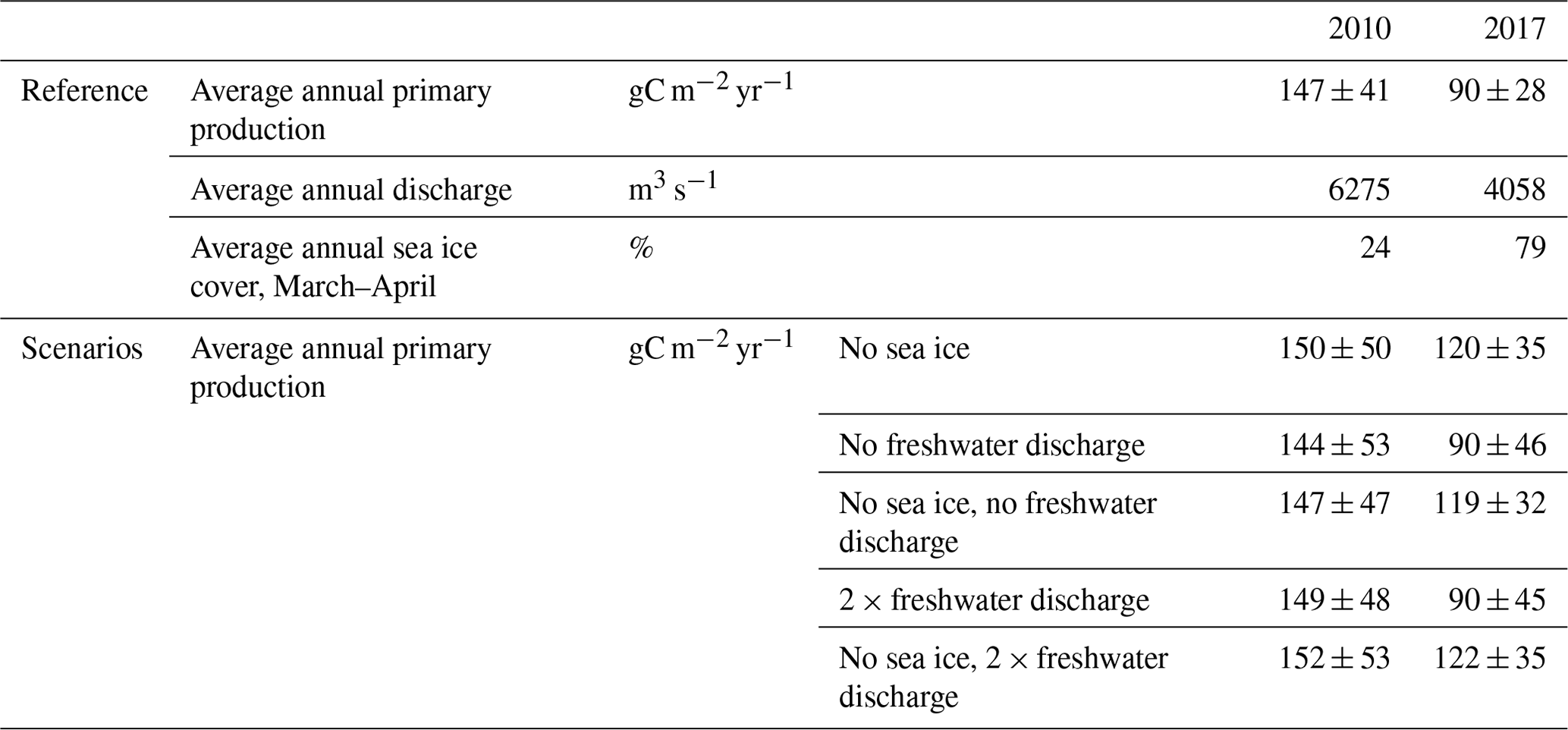
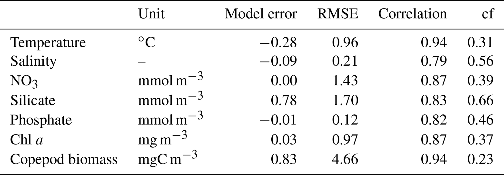
Table 2 Statistics for seasonal comparison between observational data (monthly climatology) and model data (monthly average from 2005 to 2018) at the Disko Bay station. N=12 for copepods; N=11 for temperature, salinity, and Chl a; and N=10 for other variables (see Fig. 4). All correlations were significant (p<0.01).

3 Results

3.1 Freshwater discharge and sea ice cover

Fifty years ago, the average annual liquid runoff from the ice sheet to the study area was generally ∼ 1000 m⁻³ s⁻¹ (913 ± 2214 SD m⁻³ s⁻¹, 1958–1969), whereas during the last 20 years, it has varied between 2000 and 4500 m⁻³ s⁻¹ (2591 ± 724 SD m⁻³ s⁻¹, 2000–2019; Fig. 2). The precipitation over land has also increased from about 200 (197 ± 40 SD m⁻³ s⁻¹) to 400–500 m⁻³ s⁻¹ (469 ± 77 SD m⁻³ s⁻¹). The calving of solid ice from the glaciers has only been estimated for the last 30 years, but it also shows an increasing trend; however, since the maximum in 2013, the production of ice has been lower (Fig. 2). Thus, for all three sources of freshwater, the overall long-term trend is an increase, but for the model period between 2004 and 2018, no trend was evident (Fig. 3e). The freshwater discharge from solid ice was relatively constant across the year, whereas the liquid contribution peaked during summer, from June to August, and dropped to almost zero in the winter (Fig. 3f).

The sea ice cover in Disko Bay has generally decreased over the last 35 years (Fig. 2). However, the last 15 years have been characterized by large interannual variation, with some years having virtually no ice and others having sea ice cover, as in the 1990s. During the model period, the ice generally did not form before late December, and the maximum ice cover was seen in March (Fig. 3).

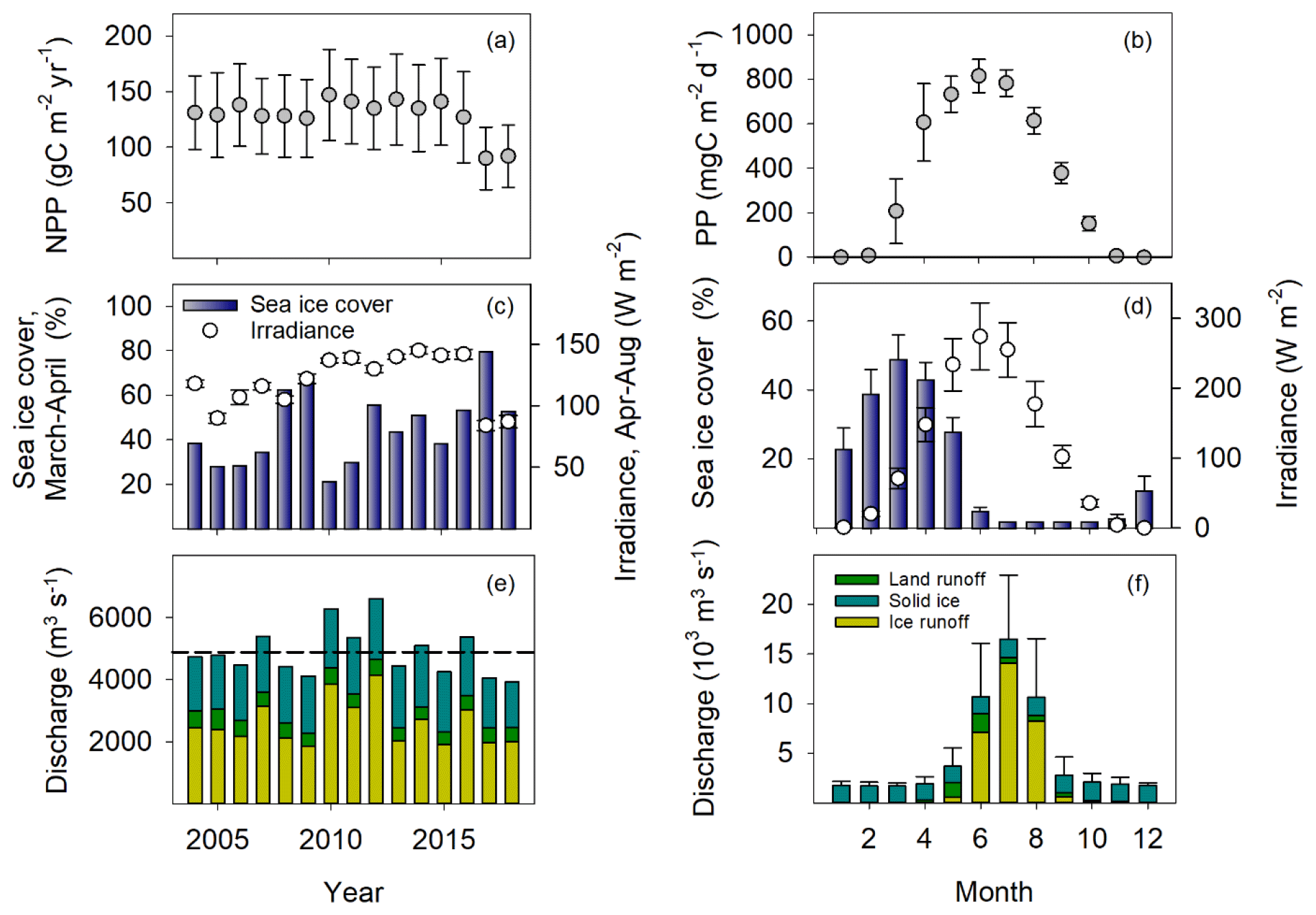
Figure 3 Primary production, sea ice cover, and freshwater discharge in Disko Bay from 2004–2018. Primary production and sea ice cover are assessed in the red square in Fig. 1, whereas the freshwater discharge is from the full model domain. (a) Average annual primary production (gC m⁻² yr⁻¹) ± SD (variation between model grid cells). (b) The average monthly primary production (mgC m⁻² d⁻¹) ± SD (variation between years) – light is averaged from the Arctic station (2010–2019). (c) The annual average sea ice cover in March and April (%). (d) The average monthly sea ice cover (%). (e) The average annual freshwater discharge (m³ s⁻¹). (f) The average monthly freshwater discharge (1000 m³ s⁻¹).

Table 3 Statistics for the spatial comparison between remote sensing data and surface model data for spring (April–June) and summer (July–September) in 2010 and 2017. In spring 2017, only June is included due to ice cover in April–May. N=6145, and all correlations were significant (p<0.01).

3.2 Validation of the model

The seasonal timing and general levels of temperature, salinity, nutrients, Chl a, and mesozooplankton agreed well with the data climatology from the field sampling south of Disko Island (Fig. 4, Table 2). All correlations between observational and model data were significant (R>0.82). The model performance assessed by the average cost function (cf) was very good for all parameters. Modeled Chl a showed the highest interannual variability in spring, and the chlorophyll bloom was somewhat too weak (∼ 30 % less) while the winter silicate was too high relative to the climatological mean observations.

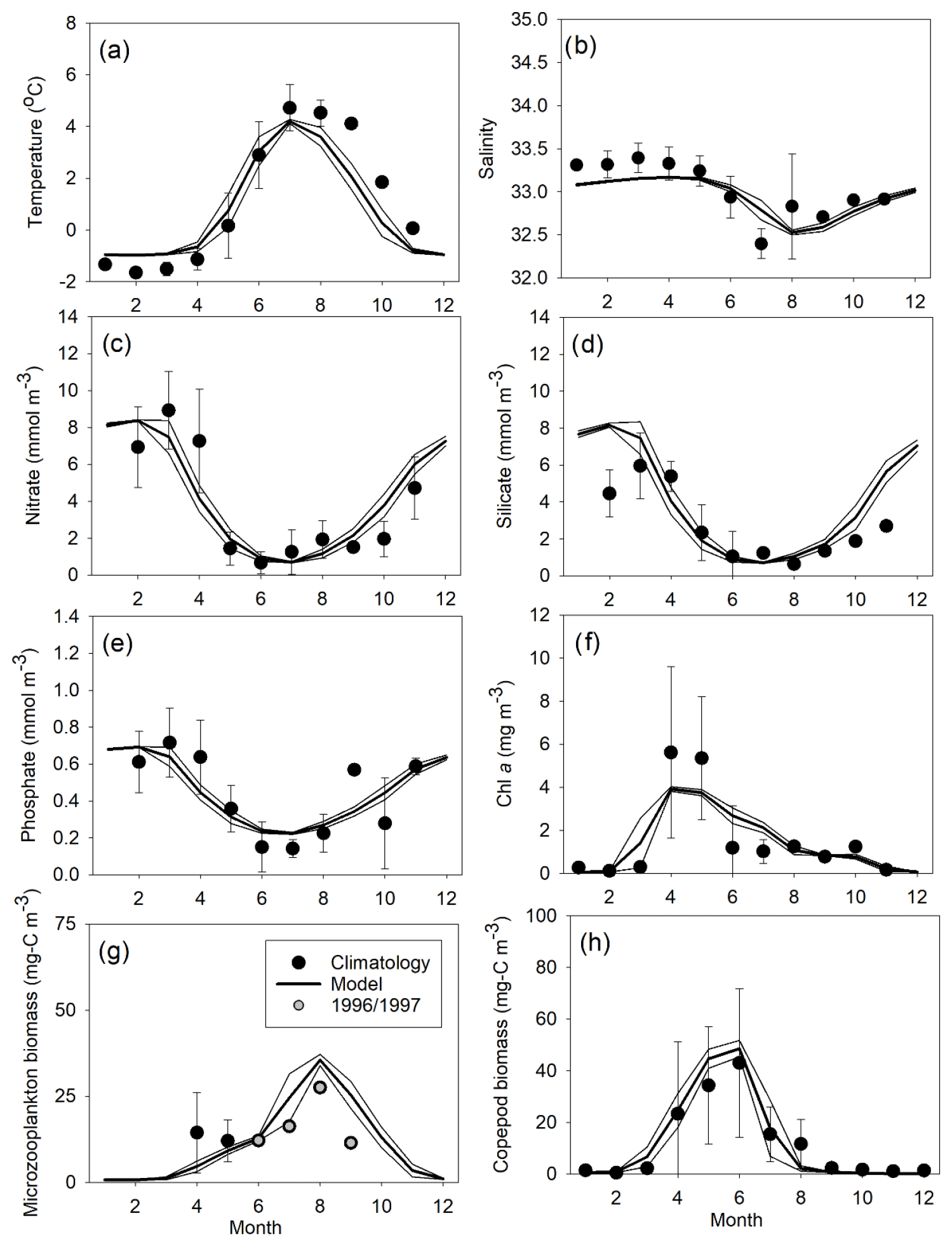
Figure 4 Comparison of monthly means (± SD) of observations and model data (2004–2018) at 69^∘ 14^′ N, 53^∘ 23^′ W for (a) temperature (^∘C), (b) salinity, (c) nitrate (mmol m⁻³), (d) silicate (mmol m⁻³), (e) phosphate (mmol m⁻³), (f) Chl a (mg m⁻³), (g) microzooplankton biomass (mgC m⁻³), and (h) mesozooplankton biomass (mgC m⁻³). Means are averaged over 0–20 m depth, except for mesozooplankton, which is averaged over 0–50 m.

The spatial distribution patterns of Chl a and temperature at the surface were compared to satellite estimates for the two years, 2010 and 2017, used in the scenarios representing low and high sea ice cover, respectively (Table 3, Fig. S1). The correlations were significant for all relations (p<0.01), and the cf number was very good or good for all (Table 3). Surface temperature tended to be higher in spring and lower in summer in the model compared to in the satellite estimates. Chl a concentrations were generally higher in the model than in the satellite data, especially in spring 2017 (Fig. S1).

3.3 Seasonal and spatial patterns of NPP in Disko Bay

Primary production starts as sea ice cover decreases and irradiance increases in February (Fig. 3). Extensive sea cover may reduce light availability in the water column and thereby limit production, and the interannual variation in NPP is highest in April because of the variation in sea ice cover, causing light availability in the water to vary accordingly. The highest NPP was in May and June at about 800 mgC m⁻³ d⁻¹ when light influx was highest and when sea ice was entirely melted (Fig. 3).

The impact of sea ice is illustrated by comparing a year with low (2010) and high (2017) sea ice cover – the spring bloom is about 25–30 d earlier in 2010 than in 2017 (Fig. 5). Comparing a station close to and far from the glacier illustrates the potential impact of the freshwater peak in late summer, as NPP is 2–3 times higher during this period at the station close to the glacier (Fig. 5).

Concerning the spatial distribution in the spring period (March–June), high NPP was seen across the bay, with the lowest values having been found southeast of Disko Island and southwest of the bay following the bathymetry. In the later summer period (July–October), primary production was more confined to the coast (Fig. 6).

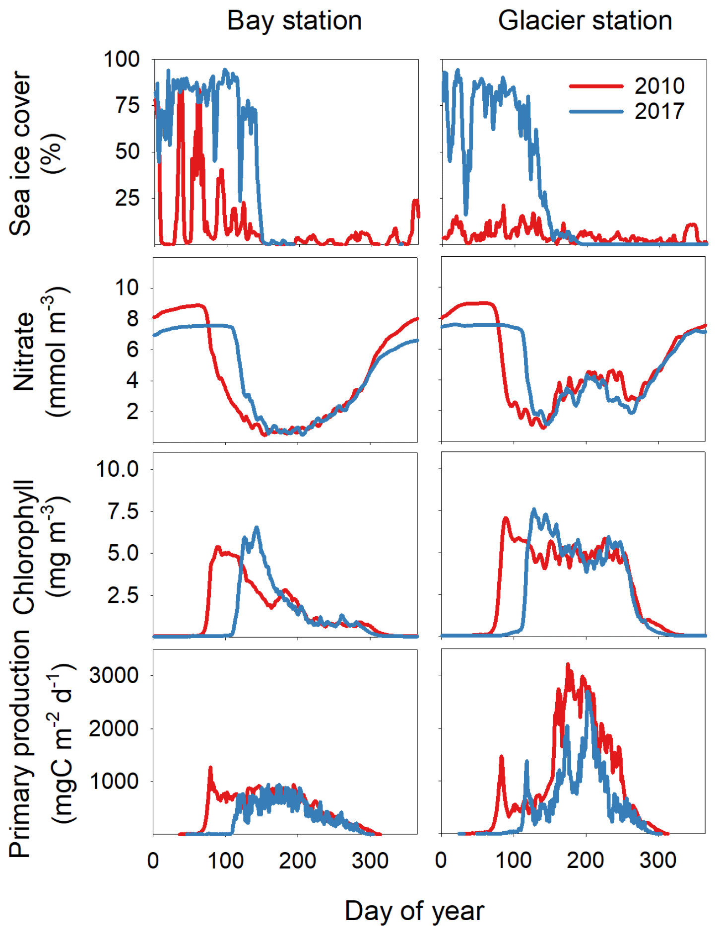
Figure 5 Sea ice cover (%), average nitrate concentration at 0–30 m (mmol m⁻³), average Chl a concentration at 0–30 m (mg m⁻³), and primary production (mgC m⁻² d⁻¹) at a station in the open bay (bay station) and at a station close to the glacier (glacier station) (Fig. 1) in 2010 and 2017.

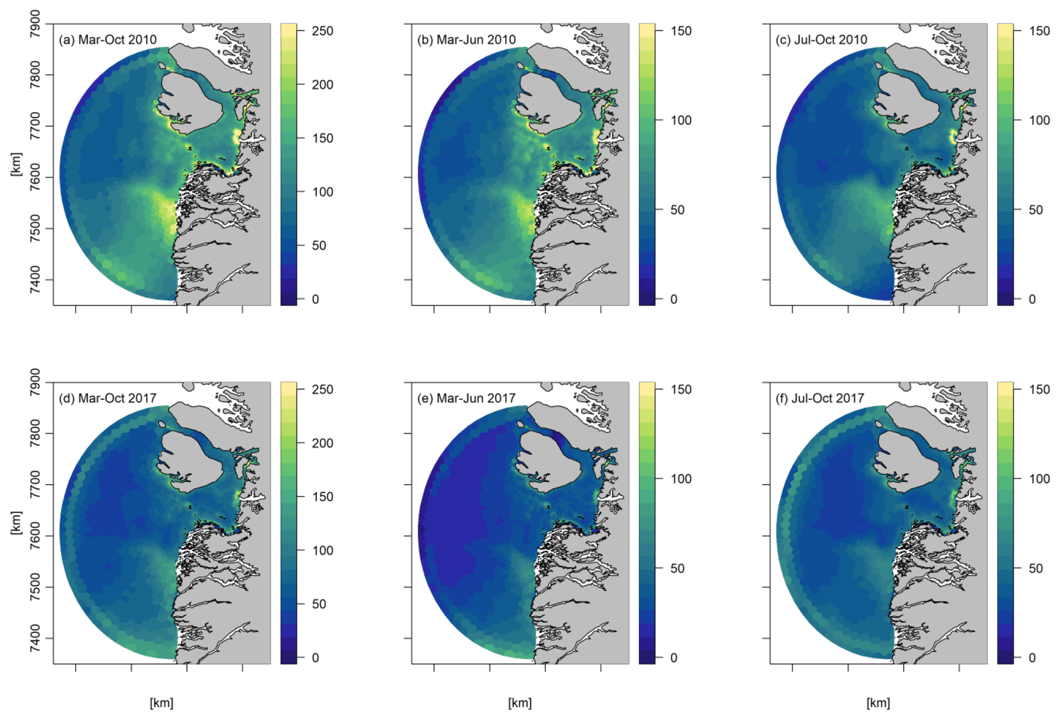
Figure 6 Average spatial distribution of primary production (gC m⁻²) in 2010 and 2017 for the periods (a, d) March–October, (b, e) March–June, and (c, f) July–October.

3.4 Annual variability of NPP

The annual average NPP in the bay estimated from the model varied between 90 and 147 gC m⁻² yr⁻¹, with an average of 129 ± 16 (SD; Fig. 3). Generally, years with high sea ice cover in spring had lower average annual NPP (Fig. 3 – Pearson product moment correlation coefficient $r=-\mathrm{0.63}$, p=0.01), while higher discharge was associated with higher annual primary productivity (Fig. 3 – r=0.51, p=0.05).

To evaluate the spatial dependency, we performed an analysis of the correlation between the sea ice cover in March–April and the annual NPP in each model grid cell. This showed a negative relationship that was widespread in the model domain – i.e., the more the sea ice, the lower the NPP (Fig. 7). One exception was in the southern part of the model domain, where the correlation was positive. The impact of the freshwater discharge on the NPP was generally positive in areas up to ∼ 50 km from the discharge and additionally in the northern part of Disko Bay, as reflected by the negative correlation with surface salinity in these areas (Fig. 7).

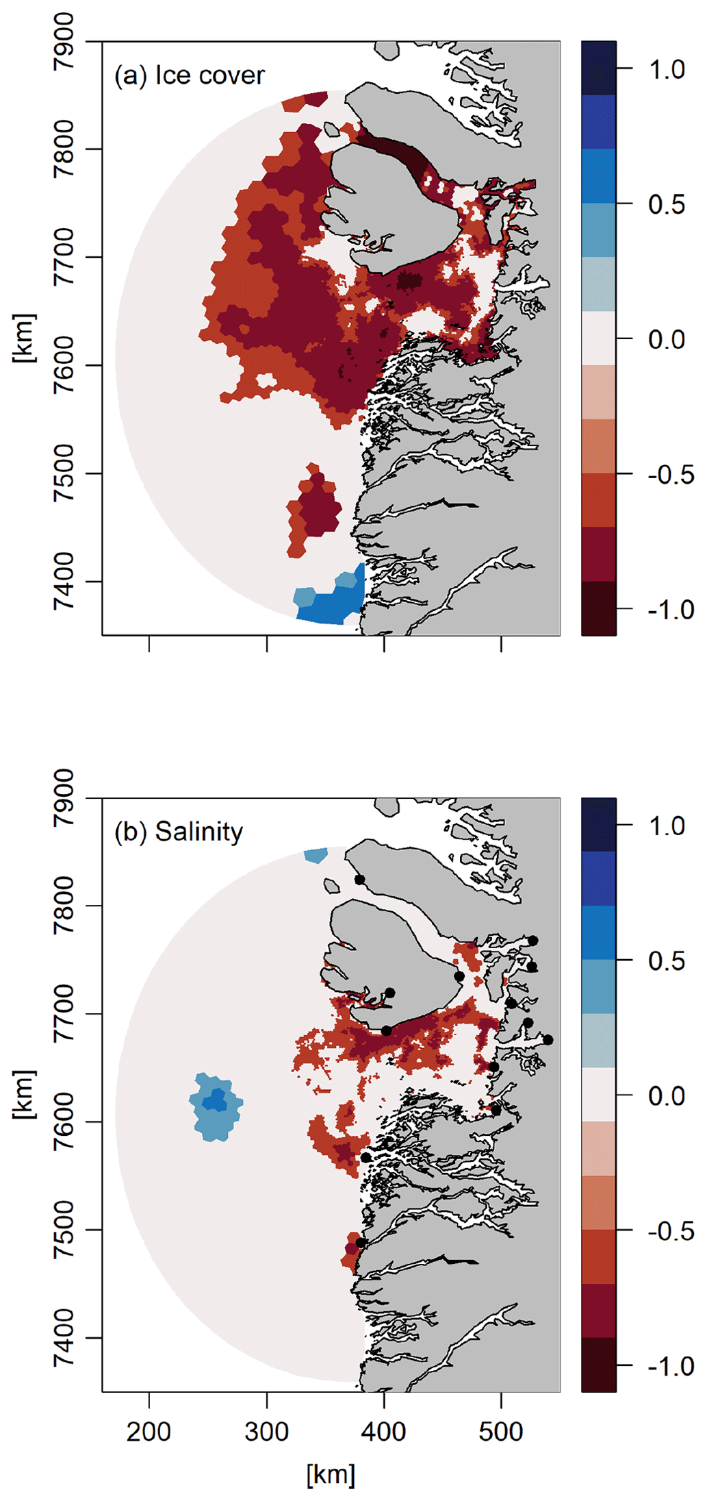
Figure 7 Correlation coefficients between the annual primary production (a) and average sea ice cover in March–April and (b) surface salinity across the period 2004–2018.

3.5 Model scenarios with sea ice cover and discharge

We studied some simple model scenarios where sea ice cover was assumed to be zero and where the discharge was either doubled or cut off; these model scenarios were based in 2010 and 2017, which had low and high sea ice cover, respectively, and opposite discharge (Fig. 3). These scenarios underline the complexity of the dynamics of the system, with some areas experiencing an increase in NPP and others experiencing a decrease (Figs. 8, 9). Furthermore, they allow us to evaluate the impact of the uncertainty of actual freshwater runoff. The year 2017 had relatively high and late ice cover (Fig. 3), and applying a scenario of no ice leads to an increase of 34 % in bay-scale annual NPP, although spatial variability is high and annual NPP changes vary between −20 % and 98 % (Fig. 9). For 2010, a year that already had low sea ice cover, the same scenario led to minor changes in the annual NPP on the bay scale (2 %; Fig. 8). For both years, the omission of freshwater discharge generally led to a decrease in annual NPP; this effect was small on the bay scale (−2 % to 0 %) but reached −64 % in near-coastal areas under glacial and/or runoff influence. Similarly, the effect of doubling the discharge was minor on the bay scale (0 %–1 %) but reached up to 55 % and 68 % in NPP increase in runoff-influenced areas in 2010 and 2017, respectively. The effects of sea ice and freshwater discharge changes combined in an approximately additive manner (Figs. 8, 9). When the forcings from sea ice cover and freshwater discharge were set to zero in 2010 and 2017, NPP in 2017 was still 20 % smaller than in 2010. This illustrates the importance of other factors for NPP, such as wind, cloud cover, and inflow to the bay.

Horizontal (east–west) current velocity profiles at the ice edge (water depth of 241 m) of Jakobshavn Isbræ showed an outgoing westerly direction, with the highest outflow at 150–200 m depth from March to October (Fig. S4a). Vertical velocities showed an upward transport, with the highest values close to the bottom at 190–216 m depth (Fig. S4b). The scenario with no runoff (noQNP) showed weaker horizontal transports and less upwelling at the ice edge (Fig. S4). When ice runoff was released at the glacier grounding line instead of at the surface, only a small increase in horizontal and vertical velocities was found at 90–200 m depth relative to the baseline. In addition, a small spatial displacement of the primary production was seen (Fig. S5). The stratification and vertical distribution of nutrients, Chl a, and primary production did not change much; they were just established a bit further offshore in the late summer months (Figs. S3, S6). The effect on the bay primary productivity is only minor (<1 %).

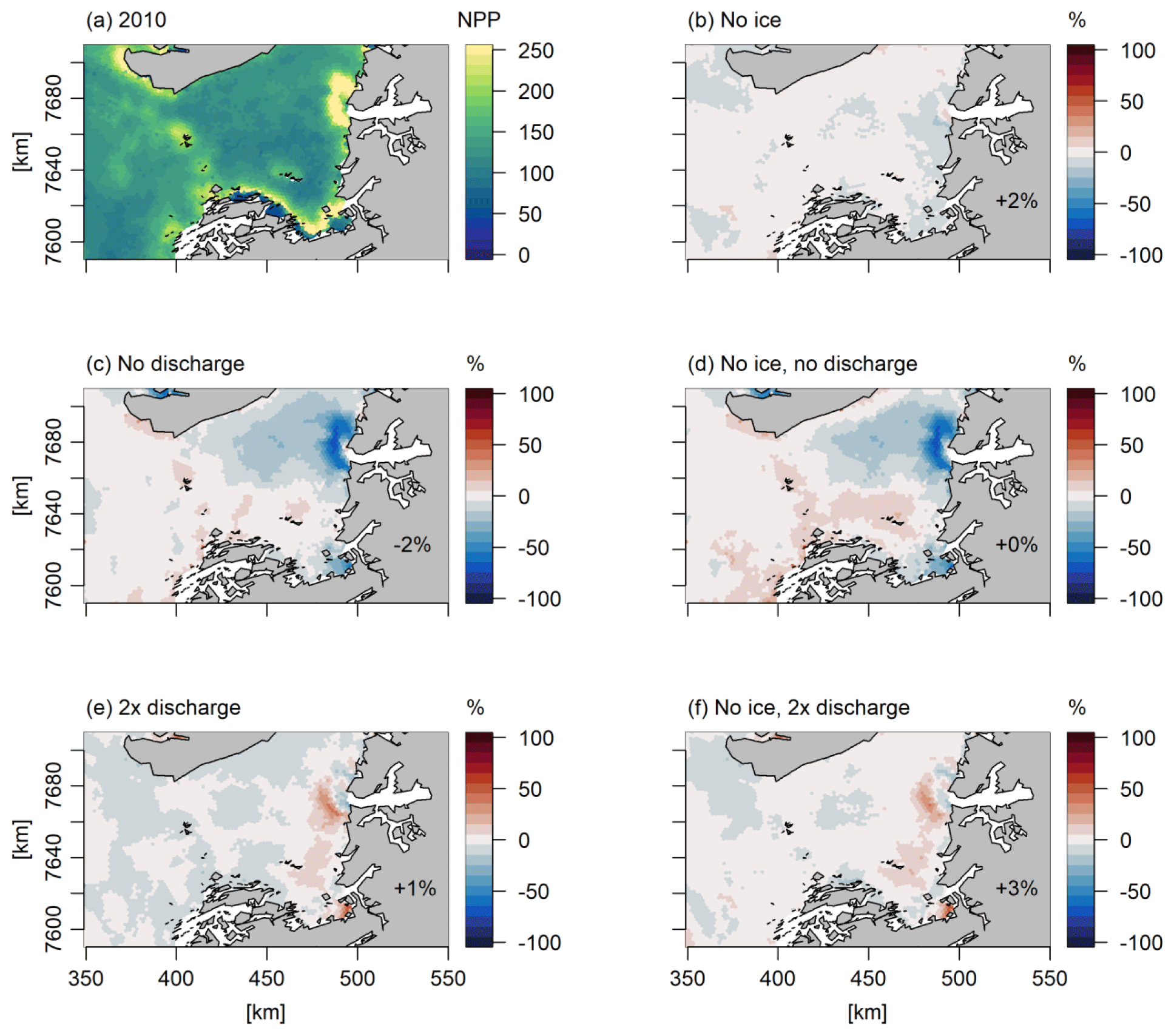
Figure 8 Response of the annual primary production to simple scenarios of changes in sea ice cover and freshwater discharge (Q) in 2010, expressed as percentage change relative to the standard model run. The percentages in the bottom of the figure are the changes in primary production in the total area shown. The following model scenarios were run (Table 1): (a) standard model run, (b) assuming no sea ice cover, (c) assuming no freshwater discharge from the Greenland ice sheet, (d) the combination of (b) and (c), (e) assuming 2 times the freshwater discharge of the standard run, and (f) the combination of (b) and (e).

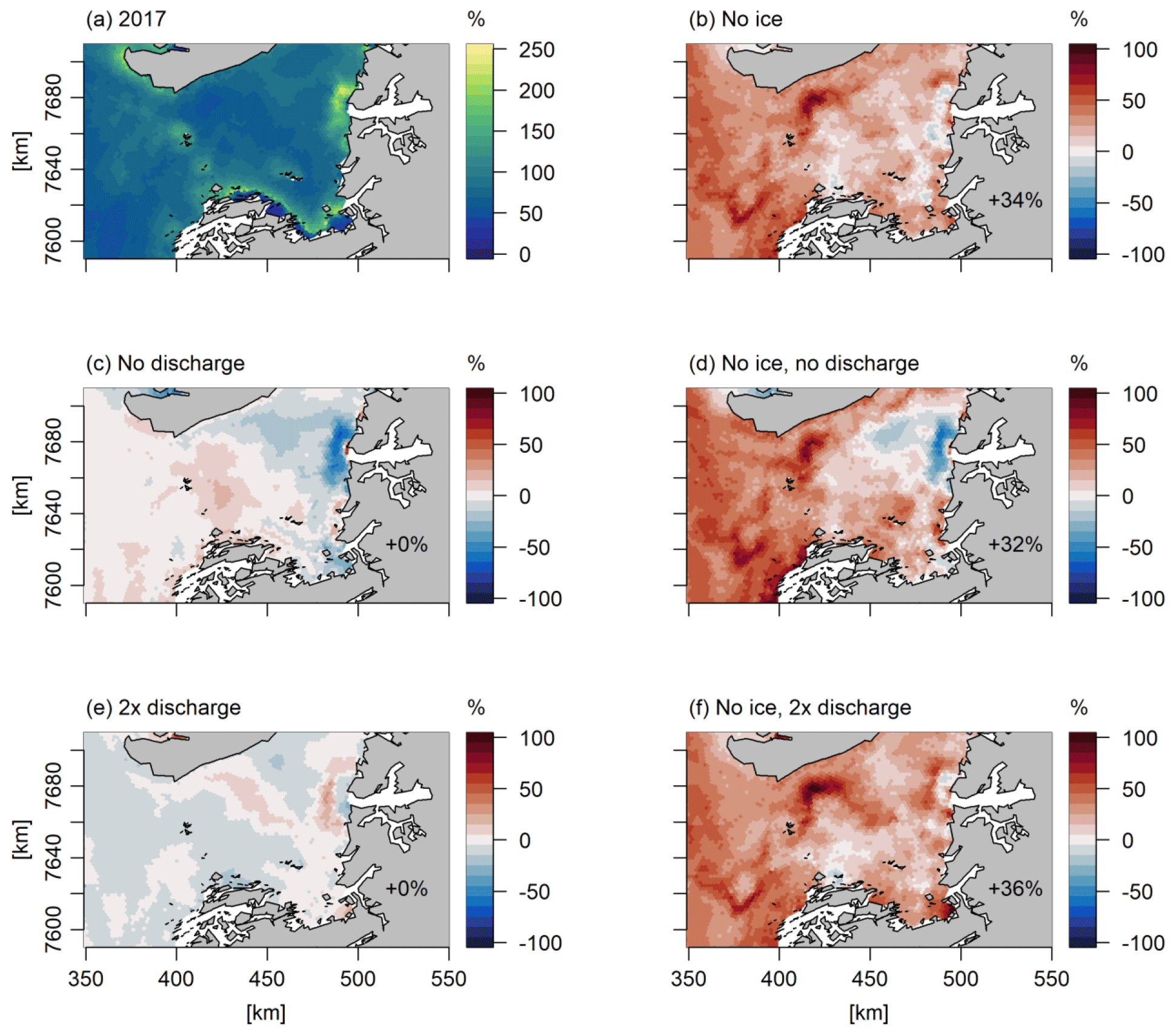
Figure 9 Response of the annual primary production to simple scenarios of changes in sea ice cover and freshwater discharge (Q) in 2017, expressed as percentage change relative to the standard model run. The percentages in the bottom of the figure are the changes in primary production in the total area shown. The following model scenarios were run (Table 1): (a) standard model run, (b) assuming no sea ice cover, (c) assuming no freshwater discharge from the Greenland ice sheet, (d) the combination of (b) and (c), (e) assuming 2 times the freshwater discharge of the standard run, and (f) the combination of (b) and (e).

4 Discussion

Primary productivity is an essential ecosystem service that shapes the structure of the marine ecosystem and fuels higher trophic levels, such as fish, that are vital for the Greenlandic society. It is therefore important to estimate potential outcomes for primary production under the continued warming and subsequent ice melt. For the coastal ocean, especially around Greenland, it is imperative to quantify how changes in sea ice cover and runoff combine to determine the availability of the two key resources, light and nitrate, that determine the magnitude and phenology of primary production. Sea ice cover and runoff influence light and nitrate availability through several intermediate processes, and their peak impact often occurs in different areas and in different months. The spatial-temporal variability and complexity of the processes involved require an approach where detailed in situ observations are combined with remote sensing and modeling. The present study is, to our knowledge, the first attempt to apply this approach to coastal Greenland.

Our model results show that a reduction in spring sea ice cover changes the plankton phenology but also increases the magnitude of annual production in Disko Bay. This suggests that there is a replenishment of nitrate into the photic zone to sustain the continued productivity beyond the initial depletion following the spring bloom. Part of the nitrate input is coupled to the runoff, but the high modeled productivity from April to July, when liquid runoff is limited, suggests that vertical mixing fueled by the wind and tide is important. That less sea ice cover will lead to increased NPP is in agreement with other studies from the open Arctic areas (Arrigo and van Dijken, 2015; Vernet et al., 2021). In other Greenland fjords, the turbulence that drives vertical mixing has been shown to be very low (Bendtsen et al., 2021; Randelhoff et al., 2020), but it seems likely that the open Disko Bay, with a tidal amplitude of up to 3 m (Thyrring et al., 2021), could have an efficient vertical flux of nitrate into the photic zone.

Our study site was chosen because Disko Bay in mid-west Greenland is considered to be a hotspot for marine biodiversity and fisheries and because it is an area where both sea ice cover and glacial runoff are likely to be important for productivity. However, regional variability is high across the coastal ocean around Greenland. For example, ice cover is very limited in most of SW Greenland and is unlikely to drive changes in future primary production, whereas glacial runoff is less in NE Greenland compared to in the rest of Greenland. Furthermore, the dominance of land- or marine-terminating glaciers, such as in Disko Bay, will be important for the outcome of increased glacial runoff on the individual-fjord scale (Hopwood et al., 2020; Lydersen et al., 2014). Finally, the winter concentration of nitrate and vertical gradients in summer differ between the east and west coasts, with low nitrate content in the East Greenland Current generally causing lower productivity compared to in west Greenland (Vernet et al., 2021).

4.1 Phenology of primary producers

A main advantage of the model is that it allows us to estimate the productivity with a higher temporal and spatial resolution than would be possible from measurements alone. The sea ice cover had a clear effect on the spring NPP. When sea ice cover is low, spring NPP starts earlier compared to years with high sea ice cover, and the largest variation in NPP between years is seen in the spring months (Fig. 3). The performed scenarios support the importance of sea ice cover; i.e., the absence of sea ice leads to a considerable increase in the annual NPP on the bay scale (Fig. 9). Potentially, NPP could start as early as February, depending on the light availability. However, an increase in NPP would also require stabilization of the water column; i.e., wind mixing would need to be sufficiently low (Tremblay et al., 2015). In contrast, the timing of the formation of the sea ice in fall is not important for the primary productivity, since the sea ice in Disko Bay does not form before the light has largely disappeared. This is in contrast to high-Arctic systems, where sea ice normally forms earlier and where a delay in the formation of sea ice in fall may result in autumn blooms (Ardyna et al., 2014).

4.2 Spatial distribution of NPP

In our analysis, we see a positive effect of the freshwater discharge on the primary productivity locally and during the summer months. This effect is related to the upwelling that is enhanced by the freshwater discharge (Figs. S2, S3). The nutrient concentration in the discharge (1.25 µM; Hopwood et al., 2020) is lower than the average concentration in the upper 30 m during summer at the station near the glacier (e.g., ∼ 4 µM NO₃) (Fig. 7) and will therefore not lead to increased NPP. This is in accordance with the general picture from glacially affected environments. River discharge may, on the other, hand carry higher nutrient concentrations, particularly of nitrogen (Hopwood et al., 2020).

We used two approaches to evaluate the spatial scale of the effect of freshwater discharge. The correlation analyses using salinity as a proxy for the discharge (Fig. 7) suggest that the discharge may have an influence up to ∼ 50 km away from the source. The scenarios where we alter the discharge suggest that the effect is only a couple of percent when considering NPP on the bay scale, whereas on a more local scale near the glacier, the importance is higher (−64 % to 147 %; Figs. 8 and 9). Godthåbsfjord is situated further south on the west coast of Greenland, and its fjord system is less directly affected by the ocean dynamics than the open Disko Bay. Here, glacial runoff has been suggested to affect the seasonal development of phytoplankton 120 km away from the glacier (Juul-Pedersen et al., 2015). Furthermore, it was found that 1 %–11 % of the NPP in the fjord systems is supported by entrainment of N by the three marine-terminating glaciers (Meire et al., 2017). Considering only the parts of the fjord directly impacted by the discharge, the estimates were 3 times higher (Hopwood et al., 2020). Analyses from Svalbard fjords impacted by glacial discharge showed positive spatiotemporal associations of Chl a with glacier runoff for 7 out of 14 primary hydrological regions but only within a 10 km distance from the shore (Dunse et al., 2022).

The modeling in this study allows us to evaluate the combined effect of changes in sea cover and freshwater discharge in the coastal ecosystem of Disko Bay. Importantly, this study also illustrates that, within the Arctic coastal zone, the combination of different climate change effects may lead to different responses within relatively small distances. Thus, while we can suggest a general increasing trend in the NPP, this may not be evident when considering local observations. This is important to consider when planning and evaluating field investigations.

4.3 Modeled NPP versus other estimates

The biogeochemical model was validated using all available observations. These are all concentrations (nutrients) or standing stocks (phytoplankton and/or zooplankton). The satisfactory validation is an indication that the rates are also adequately described. Still, it is desirable to also have direct comparison with rate measurements. There are no available NPP measurements for our modeling period. However, data are available from 1973 to 1975 (Andersen, 1981), 1996 to 1997 (Levinsen and Nielsen, 2002), and 2003 (Sejr et al., 2007). The data from 1996 to 1997 were in situ bottle incubations in the upper 30 m, and no further information on methodology was given (referred to as unpublished). The sea ice cover was generally high in Disko Bay at that time (Fig. 4), and we therefore compare the seasonal development to our model estimates from 2017, a year with extensive sea ice cover. The estimate of the annual production from 1996 to 1997 was 28 gC m⁻² d⁻¹, less than half the estimate from the 1970s (70 gC m⁻² d⁻¹) and the modeling estimate from 2017 (82 gC m⁻² d⁻¹) at the same station. The measurements do, however, both agree with the model on the seasonal timing of NPP, with an increase in NPP between March and April, and the Pearson correlation coefficients between measurements and model results were 0.84, p<0.001 (1996–1997), and 0.69, p<0.05 (1973–1975). Data from 2003 (Sejr et al., 2007) are from a shallow cove for only two shorter periods, but the production of 195 mgC m⁻² d⁻¹ in April aligns well with our estimates, whereas the value in September (27 mgC m⁻² d⁻¹) is somewhat lower.

Average estimates of NPP from Arctic glacial fjords with marine-terminating glaciers are reported to be 400–800 mgC m⁻² d⁻¹ from July to September (Hopwood et al., 2020). In the Arctic Ocean, shelf region estimates from satellite observations are 400–1400 mgC m⁻² d⁻¹ from April to September during 1998–2006 (Pabi et al., 2008). Thus, overall, our model estimates of NPP in Disko Bay of 378–815 mgC m⁻² d⁻¹ between April and September (Fig. 3) are in the same range as other estimates.

In another modeling study, a physically–biologically coupled, regional 3D ocean model (SINMOD) was compared with ocean color remote sensing (OCRS). Both OCRS and SINMOD provided similar estimates of the timing and rates of productivity of the shelves around Greenland (Vernet et al., 2021). In the region including Disko Bay, the modeled NPP was generally suggested to be much lower (20–23 gC m⁻² yr⁻¹) than our estimate (90–147 gC m⁻² yr⁻¹), and the bloom was suggested to generally start later (late May). The model by Vernet et al. (2021) mainly covered the shelf area north of Disko Bay and did not resolve the plume outside the ice fjord. Moreover, the estimates from OCRS (50 gC m⁻² yr⁻¹) were about double the modeled values and, furthermore, could only be recorded after ice break-up when the bloom was already on its maximum (Vernet et al., 2021), suggesting that it could be much higher.

4.4 Uncertainty and potential model improvement

We model the impact of turbidity on light conditions in the water column as a simple relationship between salinity and light attenuation. More sophisticated light models may be applied in future models (Murray et al., 2015). However, in a relatively open water system like Disko Bay, the effect of increased light attenuation due to increased turbidity is only expected within 5–10 km of the glacial outlet. Moreover, we do not expect an impact on the total NPP in the bay, since the nutrients will be used within the bay anyway. A comparison between the spatial distribution of surface Chl a assessed by satellite and the model showed a significant correlation, and the model performances were evaluated to be good to excellent (Table 3). Still, visual inspections of the two maps suggest that the effect of the discharge on the Chl a spatial distribution was more local and concentrated in the model than what is suggested by the satellite estimates (Fig. S1). Thus, a higher precision in the spatial distribution of the phytoplankton may be achieved by improving the model parametrization of light attenuation, e.g., by inserting a passive tracer that reflects the turbidity in meltwater. A more dynamic description of the acclimation of primary productivity to different light under nutrient conditions (Ross and Geider, 2009) may be achieved by implementing variable element ratios (e.g., C : N) of phytoplankton instead of the fixed ratios in the current model. The uncertainty in the different freshwater discharge sources may impact our estimates of marine productivity differently. Liquid runoff uncertainty and errors are more likely to be random than bias, and when averaged together (over large spatial areas or times) the uncertainty is reduced (Mankoff et al., 2020b). Conversely, solid-ice-discharge uncertainty comes primarily from unknown ice thickness, which is time invariant and therefore must be treated as a bias term (Mankoff et al., 2020a). It does not reduce when averaged in space or time.

We do not specifically model the subglacial discharge of freshwater from the marine-terminating glaciers or from melting of the numerous large icebergs in the bay. Instead, the freshwater discharge from solid ice was distributed equally across the upper 100 m in the locations where marine-terminating glaciers were present. Subglacial discharge that enters at depth will rise up the ice front by a few tens to hundreds of meters (Mankoff et al., 2016), which is within the grid cell size of the model. We therefore inserted ice discharge into the model surface layer that was found to be fully mixed in the water column during transport towards the ice edge. At the ice edge of the Jakobshavn Isbræ, modeled velocity profiles confirmed a bottom upwelling due to higher outgoing water transport at the bottom of the glacier (Fig. S4a, b) in accordance with previous studies of marine-terminating glaciers (Hopwood et al., 2020). In the scenario with no runoff (noQNP), the outgoing transport and vertical velocities at depths below 100 m were severely reduced, confirming the importance of ice discharge for the observed dynamic (Hopwood et al., 2020). When the discharge was instead inserted at the grounding line of the marine-terminating glaciers, there was a limited increase in the vertical-velocity marginal (Fig. S5b). Similarly, there was only a slight displacement of the phytoplankton bloom to further offshore and very limited changes in the stratification and vertical distribution of nutrients, Chl a, and NPP (Figs. S5, S6). The effect of the primary productivity of the bay was <1 %.

To be able to resolve the small-scale mixing between sub-glacial discharge and ambient fjord water in the plume directly in front of the glacier, a higher model resolution will be needed. A study from another Greenland fjord suggests efficient mixing near the glacial terminus, which means that the freshwater fraction in the surface water near the glacial front is only 5 %–7 %, which indicates that the mixing ratio between sub-glacial discharge and fjord water is 1 L of meltwater to 13–16 L of fjord water (Mortensen et al., 2020). The capacity of buoyancy-driven upwelling of subglacial discharge to supply nutrients to the photic zone depends on several factors including the depth of the freshwater input and the density and nutrient content of the ambient fjord water. Our approach to distribute the solid-ice freshwater input in the upper 100 m and the ice runoff in the surface layer is a first attempt to simulate the average conditions across the study area. We were able to reproduce the general pattern of upwelling (Figs. S2, S3) and the spatial dynamics of productivity, but the magnitude could be under- or overestimated. Models of high spatial and process resolution are mainly developed to describe the transports of heat and salt to glacial ice in order to estimate the melt (Burchard et al., 2022). If the focus is to describe the fine-scale processes in front of the glacier, the development within these models may be implemented in ocean models in the future.

5 Conclusions

Two important drivers of change in the Arctic coastal ecosystems are sea ice cover and glacial freshwater discharge. This modeling study estimates the response of the pelagic net primary production (NPP) to changes in sea ice cover and freshwater runoff in Disko Bay, west Greenland, from 2004 to 2018. The difference in annual production between the years with the lowest and highest annual NPP was 63 %. Our analysis suggests that sea ice cover was the more important of the two drivers of annual NPP through its effect on spring timing and annual production. Freshwater discharge, on the other hand, had a strong impact on the summer NPP near to the glacial outlet. Hence, decreasing ice cover and more discharge can work synergistically and increase productivity of the coastal ocean around Greenland.