Water mass transformation variability in the Weddell Sea in ocean reanalyses

This study investigates the variability of water mass transformation (WMT) within the Weddell Gyre (WG). The WG serves as a pivotal site for the Meridional Overturning Circulation (MOC) and ocean ventilation because it is the primary origin of the largest volume of water mass in the global ocean: Antarctic Bottom Water (AABW). Recent mooring data suggest substantial seasonal and interannual variability of AABW properties exiting the WG, and studies have linked the variability to the large-scale climate forcings affecting wind stress in the WG region. However, the specific thermodynamic mechanisms that link variability in surface forcings to variability in water mass transformations and AABW export remain unclear. This study explores how current state-of-the-art data-assimilating ocean reanalyses can help fill the gaps in our understanding of the thermodynamic drivers of AABW variability in the WG via WMT volume budgets derived from Walin's classic WMT framework. The three ocean reanalyses used are the following: Estimating the Circulation and Climate of the Ocean state estimate (ECCOv4), Southern Ocean State Estimate (SOSE) and Simple Ocean Data Assimilation (SODA). From the model outputs, we diagnose a closed form of the water mass budget for AABW that explicitly accounts for transport across the WG boundary, surface forcing, interior mixing and numerical mixing. We examine the annual mean climatology of the WMT budget terms, the seasonal climatology and finally the interannual variability. Our finding suggests that the relatively coarse resolution of these models did not realistically capture AABW formation, export and variability. In ECCO and SOSE, we see strong interannual variability in AABW volume budget. In SOSE, we find an accelerating loss of AABW during 2005–2010, driven largely by interior mixing and changes in surface salt fluxes. ECCO shows a similar trend during a 4-year time period starting in late 2007 but also reveals such trends to be part of interannual variability over a much longer time period. Overall, ECCO provides the most useful time series for understanding the processes and mechanisms that drive WMT and export variability in the WG. SODA, in contrast, displays unphysically large variability in AABW volume, which we attribute to its data assimilation scheme. We also examine correlations between the WMT budgets and large-scale climate indices, including El Niño–Southern Oscillation (ENSO) and Southern Annular Mode (SAM), and find no strong relationships.

1 Introduction

Antarctic Bottom Water (AABW) formation plays a key role in the climate system as it provides a pathway for the ventilation of abyssal waters, transport of nutrients and tracers (i.e., nitrogen, phosphorous and oxygen), and storage for large amounts of carbon (Ito et al., 2015). It is the coldest and densest water mass in the global ocean and comprises about 36 % of the global deep ocean volume (Johnson, 2008; Purkey and Johnson, 2013; Purkey et al., 2018). AABW is a key player in the abyssal cell of the Meridional Overturning Circulation (MOC), an essential component of the ocean circulation that has important global effects on the Earth's climate system. The MOC is responsible for transporting and redistributing heat, salt, carbon and nutrients (Talley, 2013). The abyssal cell circulation of the MOC is dependent upon surface forcing and interior mixing (Nikurashin and Vallis, 2011, 2012). Turbulent mixing sets the depth to which AABW upwells and provides a mechanism for waters to transform into AABW and circulate into the abyssal ocean (Nikurashin and Vallis, 2011, 2012; Ferrari et al., 2014; Nycander et al., 2015). The abyssal cell is ventilated through coastal polynyas and plumes of dense, high-oxygen-containing cold waters cascading down the continental boundaries (Williams, 2001).

The Weddell Gyre (WG) serves as the primary production site (supplying 40 %–50 %; Stewart, 2021) of AABW and as a major carbon sink (Brown et al., 2015). It is the most prominent gyre in the Southern Ocean and is pivotal for the MOC and for ventilating the ocean. The WG is a clockwise-flowing subpolar gyre east of the Antarctic Peninsula, driven by the wind stress curl in this region (Vernet et al., 2019). In the WG, relatively warmer deep waters from the north bring in heat; as these waters upwell they are cooled and freshened, transforming into surface water masses that become part of the sources for bottom water formation (Gordon et al., 2020).

Recent mooring data in the Weddell Sea suggest significant seasonal and interannual variability of AABW properties exiting the WG (Gordon et al., 2020). It is hypothesized that these variabilities are linked to the coupling of large-scale climate forcings – the El Niño–Southern Oscillation and the Southern Annular Mode (SAM) – through wind stress variability that leads to the variability in the WG strength and its density structure (Gordon et al., 2007; Meredith et al., 2008; Gordon et al., 2010; McKee et al., 2011; Armitage et al., 2018; Gordon et al., 2020). However, the specific thermodynamic mechanisms that link variability in surface forcings to AABW export remain unclear.

A crucial concept to understanding AABW formation variability and ultimately the variability of the MOC is water mass transformation (WMT). A water mass is defined as the water bounded by isosurfaces of a tracer. Any tracer can be used, but the most common tracers for WMT analysis are temperature, salinity and potential density. The transformation of a water mass occurs when the water mass' density is altered through irreversible thermodynamic processes. In order for the MOC to exist, water masses must change density classes as they circulate between the surface and abyss, just like North Atlantic Deep Water (NADW) and AABW. The next section provides an overview of the WMT theory and explains its value in providing insight into global ocean circulation.

While mooring observations such as described in Gordon et al. (2020) are useful for characterizing observed variability in water masses, they cannot provide a closed water mass budget, which requires dense observations of dynamic and thermodynamic fluxes in space and time. So in order to investigate the dynamics and thermodynamics of temporal variability in AABW using the WMT framework, we turn to three state-of-the-art, data-assimilating ocean reanalysis products. Such products are a useful tool in studying regions, such as the WG, that lack consistent and comprehensive observations and in investigating physical mechanisms that drive variability. While reanalyses are far from perfect representations of the ocean state, they represent the best attempt to synthesize diverse observations in a consistent way. Even if physical processes such as coastal polynyas are not always represented accurately in ocean reanalyses (Mazloff et al., 2010), there is still value in understanding their internal dynamic and thermodynamic budgets. By diagnosing WMT in these reanalyses, we can probe the relationships between ocean surface fluxes with a changing climate, how climate variability influences sea ice expansion and water mass transformation rates and how that ultimately affects the abyssal water properties and circulation of the lower MOC cell. Understanding how the deep ocean reacts to a warming climate will give us insight into how oceans will contribute to sea level rise and CO₂ content in the atmosphere. Purkey and Johnson (2010) have shown that the 80 % radiative imbalance in the atmosphere that has gone into heating the ocean has lead to a global change in abyssal heat content equivalent to adding 10 % to the total ocean heat storage, increasing rates of steric sea level rise by 8 %. The global impacts of the AABW circulation system on biological productivity and carbon and heat uptake, particularly in the context of climate change, makes AABW variability in the WG worth studying extensively (Vernet et al., 2019). With datasets as described in Sect. 3 and the WMT framework outlined by Walin (1982) (Sect. 2), we strive to provide insight into the mechanisms and drivers of MOC variability in the WG. Our study does not attempt to provide an authoritative time series of the “true” WMT and overturning variability in the WG; as the analysis shows, these three models show very different behavior. Our focus is on methods and mechanisms.

Our paper is organized as follows: in Sect. 2, the theory of WMT is introduced, and we detail how the WMT budget was calculated. In Sect. 3 we talk about the observational and model data used. Observational data from the World Ocean Atlas were compared to modeled bottom temperatures and salinities. The average, climatological and interannual variability of volume tendency, transport and transformation is discussed in Sects. 4.1, 4.2 and 5, respectively. Finally, the findings from the Sect. 5 are discussed and compared with similar studies in Sect. 6.

2 Water mass transformation theory

Here we provide a brief introduction to the WMT framework, first employed by Walin (1982). The WMT framework, in this context, allows for the separation of explicit mechanical and thermodynamic processes in ocean circulation (Walin, 1982; Groeskamp et al., 2016, 2019) due to surface fluxes, advective transport and diffusive mixing.

A water mass is defined as the water bounded by isosurfaces of a tracer. Any tracer can be used, but the most common tracers for WMT analysis are temperature, salinity and potential density. Here we use σ₂ – potential density referenced to 2000 dbar – because of its ability to characterize stratification through the deep and abyssal ocean. AABW in the WG region typically exists below 2000 m. σ₂ was computed using the Jackett and Mcdougall (1995) ocean equation of state. (For notational simplicity, henceforth we will write σ instead of σ₂.) The limitation of investigating WMT through potential density is the inability to quantify the effect of cabbeling and thermobaricity on WMT, potential misrepresentation of neutral mixing (Iudicone et al., 2008b), and the inability to distinguish water masses of the same density but different temperatures/salinity (Evans et al., 2018). Here we define the transformation of a water mass as the change in density of the fluid parcel due to its change in heat and salt content. Computing the transformation budget for a basin or a remote region, such as the Weddell Sea, can further our understanding by providing quantitative insight into the drivers of water mass variability.

The potential-density σ of seawater evolves according to

$$\begin{array}{}\text{(1)}& {\displaystyle \frac{\mathrm{D}\mathit{\sigma }}{\mathrm{D}t}}=\dot{\mathit{\sigma }}={\displaystyle \frac{\partial \mathit{\sigma }}{\partial \mathit{\theta }}}\dot{\mathit{\theta }}+{\displaystyle \frac{\partial \mathit{\sigma }}{\partial S}}\dot{S},\end{array}$$

where the factors $\frac{\partial \mathit{\sigma }}{\partial \mathit{\theta }}$ and $\frac{\partial \mathit{\sigma }}{\partial S}$ are the thermal expansion and haline contraction coefficients, respectively. This expression includes both a thermal component,

$$\begin{array}{}\text{(2)}& {\displaystyle \frac{\mathrm{D}\mathit{\theta }}{\mathrm{D}t}}=\dot{\mathit{\theta }}=G_{\mathrm{hdiff}}^{\mathit{\theta }}+G_{\mathrm{vdiff}}^{\mathit{\theta }}+G_{\mathrm{surf}}^{\mathit{\theta }}+G_{\mathrm{sw}}^{\mathit{\theta }},\end{array}$$

where $G_{\mathrm{hdiff}}^{\mathit{\theta }}$ represents the temperature tendency due to horizontal/isopycnal mixing, $G_{\mathrm{vdiff}}^{\mathit{\theta }}$ is the tendency due to vertical/diapycnal mixing, $G_{\mathrm{surf}}^{\mathit{\theta }}$ is the surface forcing and $G_{\mathrm{sw}}^{\mathit{\theta }}$ is the shortwave penetration, and a haline component,

$$\begin{array}{}\text{(3)}& {\displaystyle \frac{\mathrm{D}S}{\mathrm{D}t}}=\dot{S}=G_{\mathrm{hdiff}}^{\mathrm{S}}+G_{\mathrm{vdiff}}^{\mathrm{S}}+G_{\mathrm{surf}}^{\mathrm{S}},\end{array}$$

where the terms represent the salinity tendency due to the same non-conservative terms as for temperature, except for the shortwave radiation term. We use these forms of the heat and salt budget because they correspond to how those budgets are diagnosed from numerical simulations.

To understand the equations to come, we briefly cover the Heaviside and delta functions. The Heaviside function, ℋ, is 0 when the argument is negative and 1 for positive arguments. The Heaviside function is the integral of the delta function where

$$\begin{array}{}\text{(4)}& {\displaystyle \frac{\partial \mathcal{H}\left(x\right)}{\partial x}}=\mathit{\delta }\left(x\right).\end{array}$$

This approach allows us to define a region under a reference isopycnal ($\stackrel{\mathrm{̃}}{\mathit{\sigma }}$). The density field is a function of x,y, z and time, meaning

$$\begin{array}{}\text{(5)}& \mathit{\sigma }=\mathit{\sigma }(x,y,z,t),\end{array}$$

so that the total volume of water denser than $\stackrel{\mathrm{̃}}{\mathit{\sigma }}$ within a region R is given by

$$\begin{array}{}\text{(6)}& \mathcal{V}(\stackrel{\mathrm{̃}}{\mathit{\sigma }},t)=\underset{R}{\int }\mathcal{H}(\stackrel{\mathrm{̃}}{\mathit{\sigma }}-\mathit{\sigma })\mathrm{d}V,\end{array}$$

i.e., the cumulative volume distribution.

The WMT budget for region R in the following equation, expresses the relationship between the time evolution 𝒱 to the inflow/outflow transports (Ψ) on the basin boundary plus the thermodynamic transformation (Ω) occurring in the basin interior:

$$\begin{array}{}\text{(7)}& {\displaystyle \frac{\partial \mathcal{V}}{\partial t}}=\mathrm{\Psi }+\mathrm{\Omega },\end{array}$$

where

$$\begin{array}{}\text{(8)}& \mathrm{\Psi }(\stackrel{\mathrm{̃}}{\mathit{\sigma }},t)=-\underset{\mathit{\delta }R}{\int }(\mathit{u}\cdot \widehat{\mathit{n}})\mathcal{H}(\stackrel{\mathrm{̃}}{\mathit{\sigma }}-\mathit{\sigma })\mathrm{d}A\end{array}$$

(δR is the region boundary and $\widehat{\mathit{n}}$ is the unit normal on the boundary) and

$$\begin{array}{}\text{(9)}& \mathrm{\Omega }(\stackrel{\mathrm{̃}}{\mathit{\sigma }},t)=-\underset{R}{\int }\mathit{\delta }(\stackrel{\mathrm{̃}}{\mathit{\sigma }}-\mathit{\sigma })\dot{\mathit{\sigma }}\mathrm{d}V.\end{array}$$

The $\dot{\mathit{\sigma }}$ in Eq. (9) comes from the potential-density conservation equation (Eq. 1). It represents the sum of the temperature and salinity components (Eqs. 2 and 3, respectively) of the non-conservative tendencies from horizontal and vertical diffusion, surface forcing and shortwave penetration (potential temperature only) (Abernathey et al., 2016, their Supplement). The WMT framework helps us discern the contributions to the water mass variability by quantitatively relating it to the driving processes of surfacing forcing and advective transport to interior mixing.

Numerical implementation

In order to assess the mechanisms behind AABW transformation and circulation variability, a fully closed WMT budget is desirable. To calculate this, we must first close the temperature and salinity budgets. WMT volume budget analysis was conducted using Estimating the Circulation and Climate of the Ocean (ECCO), Southern Ocean State Estimate (SOSE), and Simple Ocean Data Assimilation (SODA) reanalysis data. In all of these cases, the ocean is divided into discrete layers ${\stackrel{\mathrm{̃}}{\mathit{\sigma }}}_n$, and each of the relevant terms is calculated inside these discrete layers. The discrete analog of the cumulative volume integral (Eq. 6) is

$$\begin{array}{}\text{(10)}& \mathcal{V}({\stackrel{\mathrm{̃}}{\mathit{\sigma }}}_n,t)=\sum _{i,j,k}\mathrm{\Delta }V\mathcal{H}({\stackrel{\mathrm{̃}}{\mathit{\sigma }}}_n-\mathit{\sigma }),\end{array}$$

where the summation is over each model grid cell within the region of interest and ΔV is the finite volume of each cell. Henceforth, we use the shorthand 𝒱=cumsum_σ(ΔV) to denote this operation.

The time rate of volume change was computed and balanced by the calculated σ total tendency (Ω_tottend) and a residual (R1) due to the discretization of isopycnal layers:

$$\begin{array}{}\text{(11)}& {\displaystyle \frac{\partial \mathcal{V}}{\partial t}}={\mathrm{\Omega }}_{\mathrm{tottend}}+R\mathrm{1},\end{array}$$

where

$$\begin{array}{}\text{(12)}& {\mathrm{\Omega }}_{\mathrm{tottend}}=-{\displaystyle \frac{\partial }{\partial \stackrel{\mathrm{̃}}{\mathit{\sigma }}}}{\mathrm{cumsum}}_{\mathit{\sigma }}\left(G_{\mathrm{tottend}}^{\mathit{\sigma }}\right)\end{array}$$

and where $G_{\mathrm{tottend}}^{\mathit{\sigma }}=(\partial \mathit{\sigma }/\partial \mathit{\theta })G_{\mathrm{tottend}}^{\mathit{\theta }}+(\partial \mathit{\sigma }/\partial S)G_{\mathrm{tottend}}^{\mathrm{S}}$ is the model's total tendency for potential density, a weighted sum of total tendencies for temperature and salinity. This term is the sum of conservative tendencies due to horizontal and vertical advection, non-conservative tendencies due to horizontal and vertical diffusion and surface forcings (including shortwave penetration for the potential temperature component). It is helpful to calculate R1 explicitly in order to determine if the chosen σ bin size is appropriate. We found that the budgets were not sensitive to changing σ bin sizes. Smaller bin sizes meant higher resolution; however, that did not significantly change R1 and increased computational costs.

Next, the total advection tendency term (Ψ_adv) is decomposed to σ's velocity component (Ψ_vel) and a residual term (R2) attributed by a yet-to-be-determined combination of numerical mixing and numerical cabbeling effects:

$$\begin{array}{}\text{(13)}& {\mathrm{\Psi }}_{\mathrm{adv}}={\mathrm{\Psi }}_{\mathrm{vel}}+R\mathrm{2}.\end{array}$$

The term

$$\begin{array}{}\text{(14)}& {\mathrm{\Psi }}_{\mathrm{adv}}=-{\displaystyle \frac{\partial }{\partial \stackrel{\mathrm{̃}}{\mathit{\sigma }}}}{\mathrm{cumsum}}_{\mathit{\sigma }}\left({\displaystyle \frac{\partial \mathit{\sigma }}{\partial \mathit{\theta }}}{G}_{\mathrm{adv}}^{\mathit{\theta }}+{\displaystyle \frac{\partial \mathit{\sigma }}{\partial S}}{G}_{\mathrm{adv}}^{\mathrm{S}}\right)\end{array}$$

represents the direct effect, as output from the models, of the advection of temperature and salinity on the total tendency of potential density in each grid cell, while

$$\begin{array}{}\text{(15)}& {\mathrm{\Psi }}_{\mathrm{vel}}=-{\mathrm{cumsum}}_{\mathit{\sigma }}(\mathit{u}\cdot \widehat{\mathit{n}}\mathit{\delta }A)\end{array}$$

is the net transport across the region boundary, accumulated in ${\stackrel{\mathrm{̃}}{\mathit{\sigma }}}_n$ bins; this is the conventional overturning streamfunction. In the continuous world, Ψ_adv and Ψ_vel can be shown to be mathematically identical. However, numerical discretization of the advection operator yields a residual term representing non-advective affects of the advection scheme. This residual has in fact been used to quantify numerical mixing in other studies (Holmes et al., 2021). Separating out the numerical residual allows us to explicitly see the volume transport of certain densities by purely physical inflow/outflow mechanisms and by a mixing term.

Water mass transformation, Ω_tf, was computed by summing the rest of the tendency terms due to non-conservative, thermodynamic processes such as diffusion, shortwave radiation and surface forcings of heat and freshwater:

$$\begin{array}{}\text{(16)}& \begin{array}{rl}{\mathrm{\Omega }}_{\mathrm{tf}}& =-{\displaystyle \frac{\partial }{\partial \stackrel{\mathrm{̃}}{\mathit{\sigma }}}}{\mathrm{cumsum}}_{\mathit{\sigma }}\left[{\displaystyle \frac{\partial \mathit{\sigma }}{\partial \mathit{\theta }}}\right(G_{\mathrm{hdiff}}^{\mathit{\theta }}+G_{\mathrm{vdiff}}^{\mathit{\theta }}\\ & +G_{\mathrm{surf}}^{\mathit{\theta }}+G_{\mathrm{sw}}^{\mathit{\theta }})+{\displaystyle \frac{\partial \mathit{\sigma }}{\partial S}}(G_{\mathrm{hdiff}}^{\mathrm{S}}+G_{\mathrm{vdiff}}^{\mathrm{S}}+G_{\mathrm{surf}}^{\mathrm{S}}\left)\right].\end{array}\end{array}$$

By defining residuals in this way, we arrive at a numerical form of Eq. (7) below, which is closed by construction:

$$\begin{array}{}\text{(17)}& {\displaystyle \frac{\partial \mathcal{V}}{\partial t}}={\mathrm{\Psi }}_{\mathrm{vel}}+R\mathrm{2}+{\mathrm{\Omega }}_{\mathrm{tf}}+R\mathrm{1}.\end{array}$$

Since R2 represents numerical mixing, we can more concisely write Eq. (17) to be

$$\begin{array}{}\text{(18)}& {\displaystyle \frac{\partial \mathcal{V}}{\partial t}}={\mathrm{\Psi }}_{\mathrm{vel}}+{\mathrm{\Omega }}^{\ast }+R\mathrm{1},\end{array}$$

where

$$\begin{array}{}\text{(19)}& {\mathrm{\Omega }}^{\ast }={\mathrm{\Omega }}_{\mathrm{tf}}+R\mathrm{2}.\end{array}$$

We can even further decompose the various G_surf terms by breaking them into different sub-components. One such analysis we do here is to separate $G_{\mathrm{surf}}^{\mathrm{S}}$ into a component directly related to sea ice and a component due to direct exchange of freshwater with the atmosphere and land, as done also by Abernathey et al. (2016). We found a minimal contribution of E–P–R to surface salt fluxes and a dominant role from sea ice activity. Specifically, we saw brine rejection activity throughout most of the season until summer when there were spikes in ice melt during a few summer months (amplitude usually matching the highest brine rejection spike). SODA does not provide any tendency diagnostics; however, it does provide the velocity field. Thus, in SODA we simply define Ω^∗ via the residual: ${\mathrm{\Omega }}^{\ast }=\partial \mathcal{V}/\partial t-{\mathrm{\Psi }}_{\mathrm{vel}}$.

Equation (17) represents the WMT volume budget expressed by explicit terms due to physical and thermodynamic processes captured by the model. Now we can see the time rate of volume change is balanced by the physical transport into and out of the WG, plus the residual mixing term, the transformation term and the numerical discretization residual. Subsequent plots in Sects. 4.1, 4.2 and 5 display each term's contribution to the total WMT volume budget.

3 Data and models

The observational data and numerical simulations used in this project are described here. The strengths and limitations of the models are mentioned in each section, and the evaluation of each numerical model is discussed in Sect. 3.5.

3.1 World Ocean Atlas

We used observational temperature and salinity as a baseline for validating the use of each model. The evaluation of each model compared with observations is in Sect. 3.5. The observational temperature and salinity data are from the World Ocean Atlas 2013 (WOA) (Locarnini et al., 2013; Zweng et al., 2013). WOA is a set of objectively analyzed 1^∘ gridded climatological fields of in situ temperature and salinity. The 1^∘ climatological fields averaged over 2005–2012 are presented in this paper as a means for model validation assessment.

Temperature and salinity profile data were obtained from bottled samples; ship-deployed conductivity–temperature–depth (CTD); mechanical, digital and expendable bathythermographs (XBT); profiling floats; moored and drifting buoys; gliders; undulating oceanographic recorder (UOR); and pinniped mounted CTD sensors. WOA contains both observed-level profile data and standard depth profile data with various quality control flags applied. In most regions with sparse data coverage, such as the WG region, flagged data seen as outliers were not removed because they may still represent legitimate values, and they are therefore, included in the climatological periods used here (Locarnini et al., 2013; Zweng et al., 2013).

3.2 Estimating the Circulation and Climate of the Ocean

ECCO version 4 release 3 state estimate is a reconstruction of the 3-D time-varying ocean and sea ice state (Forget et al., 2015). Produced from MITgcm, ECCO has an approximately 1^∘ horizontal grid resolution and 50 vertical levels of varying thickness. It provides monthly-averaged 3-D ocean, sea ice and air–sea flux fields; 2-D daily-averaged ocean and sea ice fields; and 6-hourly atmosphere fields, all covering the period 1 January 1992 to 31 December 2015.

The ECCO state estimate provides a statistical best fit to observational data; however, unlike other ocean reanalyses that directly adjust the model state to fit the data, such as SODA, described in Sect. 3.4, ECCO is a free-running model that simulates what is observed in the ocean based on the governing equations of motions, a set of initial conditions, parameters and atmospheric boundary conditions. Some observational data ECCO uses are from Argo floats, shipboard CTD and XBT measurements, marine mammals, mooring data, the Radar Altimeter Database System, satellite products from the National Snow and Ice Data Center (NSIDC), and programs such as SSM/I DMSP-F11 and SSM/I DMSP-F13 and SSMIS DMSP-F17 (Fukumori et al., 2018).

The ECCO state estimate satisfies physical conservation laws, with no unidentified sources of heat and buoyancy. Due to the model's dynamically consistent nature, it conserves heat, salt, volume and momentum (Wunsch and Heimbach, 2007, 2013); the state estimate can be used to explore the origins of ocean heat, salt, mass, sea ice and regional sea level variability (Forget et al., 2015). It uses a nonlinear free surface combined with real freshwater flux forcing and the scaled height coordinate, and users of ECCO are able to assess model–data misfits (Forget et al., 2015). Known issues of the state estimate are mentioned for the first release in Forget et al. (2015). For example, ECCO has residual systematic errors, especially in regions with sparse data (Buckley et al., 2017).

3.3 Southern Ocean State Estimate

SOSE is a model-generated best fit for Southern Ocean observations (Mazloff et al., 2010). It is a solution to the MITgcm, constructed in spherical coordinates with 42 vertical levels of varying depth (m) and a C-gridded dataset at a $\mathrm{1}/\mathrm{6}$^∘ horizontal resolution, available at timestamps daily and annually (Mazloff, 2008). Its iteration runs at 5 d averages starting from 1–5 January 2005 and ending on 31 December 2010.

SOSE is also a data-assimilating model. It uses similar observation data as ECCO. Observations of daily sea ice concentration have been attained from the NSIDC. Some limitations are similar to that of reanalyses with regard to regions and variables being more reliable, with more observations covered in those areas, and the opposite being true for regions with sparse data. SOSE provides a self-consistent state estimate that satisfies momentum, volume, heat and freshwater conservation. Some of its key strengths are that SOSE has a better spatial and temporal resolution than most state estimate models and is the highest-resolution model used in this study. It is dynamically consistent and best-fit to the available 190 observations, and its biases are well-documented (Mazloff and National Center for Atmospheric Research Staff, 2021).

This study examines the Weddell Sea region, and so far one major bias has been found during our analysis: SOSE produces an open-ocean polynya in the first year of its run (2005) which was not observed in the real ocean; therefore, this year is removed from the time mean and climatology, but the anomalous interannual variability still includes the year 2005.

3.4 Simple Ocean Data Assimilation

SODA ocean/sea ice reanalysis is the third numerical model used for our water mass transformation analysis. The SODA3 reanalyses are built on the Modular Ocean Model, version 5, ocean component of the Geophysical Fluid Dynamics Laboratory CM2.5 coupled model (Delworth et al., 2012), with fully interactive sea ice at a 0.25^∘ × 0.25^∘ horizontal and 50-level vertical resolution (Carton et al., 2018). The sea ice data are taken from the Geophysical Fluid Dynamics Lab's Sea Ice Simulator model (Delworth et al., 2012). They do not include flow of ice from continental regions into the ocean, including ice shelves and their interaction with the ocean. Improvements have been made in SODA3 such as upgrades to the sea surface temperature (SST) datasets and a 40 % increase in hydrographic data from the latest release of the World Ocean Database. Earlier generations of ocean reanalysis have contained systematic errors that have several sources, including measurement bias, inaccurate model physics and numerical resolution, and biases in fluxes and initial conditions. The release of SODA3 was an effort to address these broad issues; for example, the adoption of the iterative flux correction procedure of Carton et al. (2018) addresses the bias in surface forcing in which flux error is estimated from the misfits obtained from an initial ocean reanalysis to alter fluxes for a revised ocean reanalysis. SODA3 was also upgraded to be an ensemble reanalysis, for which the ensemble spread provides an estimate of uncertainty. A comparison to ORAS5 and ECCO is provided in (Carton et al., 2019).

SODA3 is included with finer eddy-permitting spatial resolution, active sea ice and bias adjustment. The version this study uses is SODA3.4.2 (SODA henceforth), which means that the assimilated data are restricted to the basic hydrographic data and SST with meteorological forcing derived from the European Centre for Medium-Range Weather Forecasts interim reanalysis (ERA-Interim) daily average surface radiative and state variables (Dee et al., 2011) and the COARE4 bulk formula with flux bias correction applied. The ocean and ice data run every 5 d from 4 January 1993 to 19 December 2019 and the transport files every 10 d from 7 January 1993 to 17 December 2019. There were jumps in the salt field from the ocean files occurring before 1997 that we suspect are the result of the reanalysis's nudging technique. For this reason, we have used SODA running from 15 February 1997 to 17 December 2019.

The biggest difference between SODA, ECCO and SOSE is their method of data assimilation. ECCO and SOSE use the adjoint data assimilation method, which optimizes the initial conditions and model parameters by incorporating observation data to a physics-based numerical simulation. The SODA experiment uses an optimal interpolation method for their data assimilation, in which the ocean state is constructed from a forecast using a linear deterministic sequential filter and based on the difference between observations and the forecast mapped onto the observation variable and its location (Carton et al., 2018). Due to the method of data assimilation, it is not possible to diagnose a closed heat budget in SODA, and therefore we cannot explicitly calculate Ω. However, we can calculate $\partial V/\partial t$ and Ψ. So in the following analysis, we infer Ω as a residual.

3.5 Model assessment

It is well known that numerical models struggle to capture the complex physics on the Antarctic shelves that determine AABW properties and circulation (Heuzé et al., 2013). Although these models assimilate data, they are still constrained by their resolution and physical parameterizations. In this section we assess each model against the World Ocean Atlas data. This step gives a base for assessing each model's reliability in simulating ocean physics in a region with limited observational data, such as the Weddell Sea region. Such validation was assessed by comparing bottom temperature and salinity spatial distributions, as well as time-averaged temperature–salinity (TS) distributions, in the WG region between ECCO/SOSE/SODA and WOA. ECCO and SODA were averaged over the same time period as the WOA product (2005–2012) except for SOSE, whose time period only spans 2005–2010. Noting that the time period between SOSE and observation is different, we still execute the comparison with what is available but recognize that this introduces unknown biases to our comparison. The boundaries of the WG region are defined here to be from 65^∘ W to 30^∘ E and from 78 to 57^∘ S (Gordon et al., 2007; Neme et al., 2021).

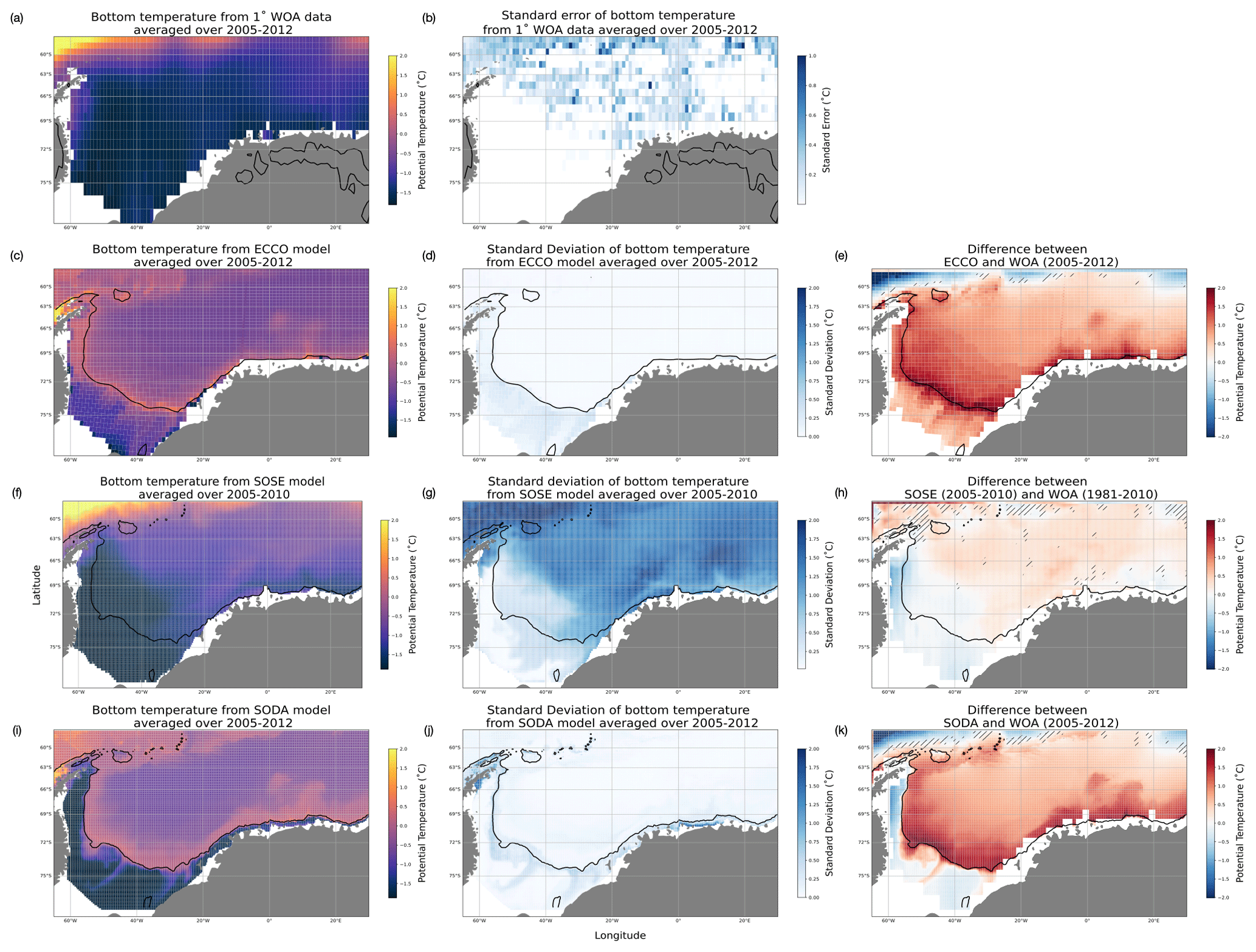
Figure 1 Annual mean of bottom temperatures (^∘C) of the Weddell Gyre region for (a) WOA (2005–2012), (c) ECCO (2005–2012), (f) SOSE (2005–2010) and (i) SODA (2005–2012). Standard error of WOA observations is shown in (b); temporal standard deviations are shown for (d) ECCO, (g) SOSE and (j) SODA. The differences between the observed and simulated bottom temperatures are shown in (e) ECCO, (h) SOSE and (k) SODA. Black hatching denotes the areas where the difference between model and WOA is less than the observation's standard error. The black contour represents the 1000 m isobath.

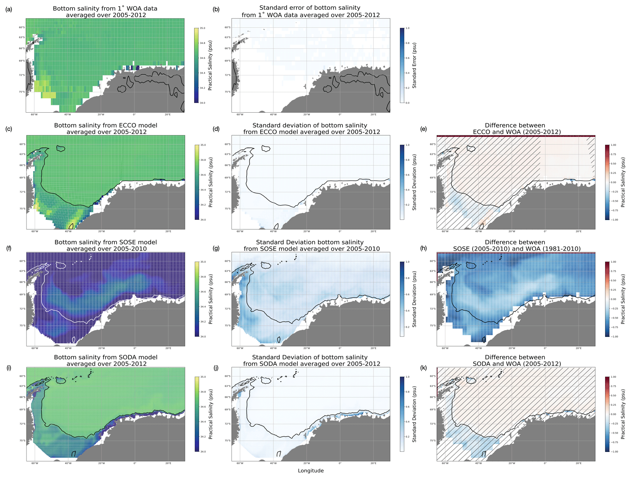
Figure 2 Annual mean of bottom salinity (psu) of the Weddell Gyre region for (a) WOA (2005–2012), (c) ECCO (2005–2012), (f) SOSE (2005–2010) and (i) SODA (2005–2012). Standard error of WOA observations is shown in (b); temporal standard deviations are shown for (d) ECCO, (g) SOSE and (j) SODA. The differences between the observed and simulated bottom salinities are shown in (e) ECCO, (h) SOSE and (k) SODA. Black hatching denotes the areas where the difference between model and WOA is less than the observation's standard error. The black contour represents the 1000 m isobath.

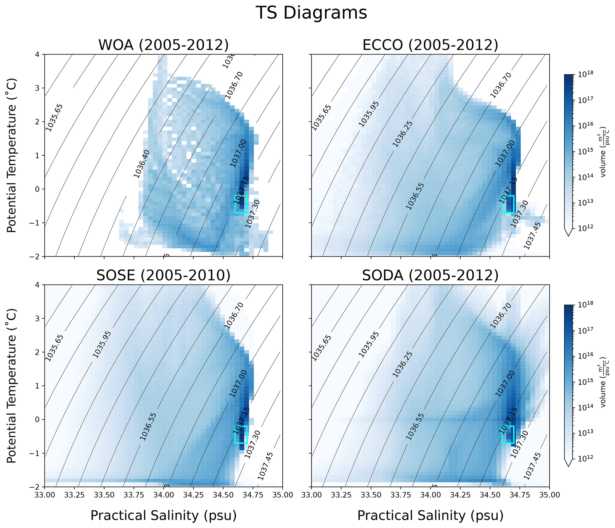
Figure 3 Averaged temperature–salinity distribution of the WG region for WOA, ECCO, SODA (2005–2012) and SOSE (2005–2010). Contour lines represent potential density referenced at 2000 m (σ₂). The cyan box shows the temperature–salinity range of AABW.

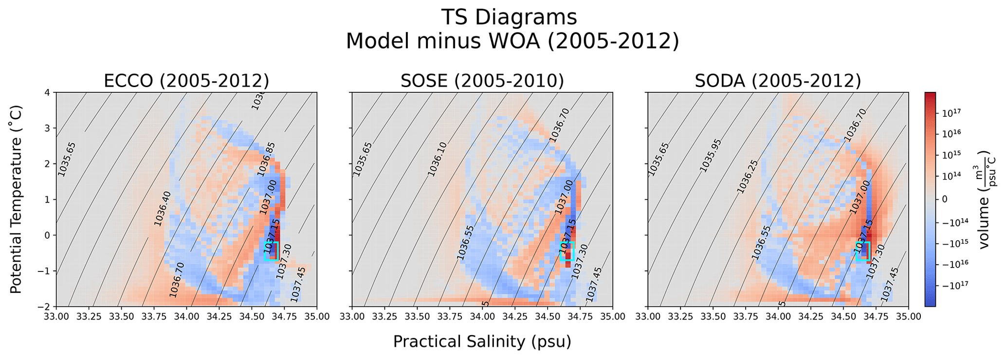
Figure 4 Averaged temperature–salinity distribution of the difference between WOA and each model. Contour lines represent potential density referenced at 2000 m (σ₂). The cyan box shows the temperature–salinity range of AABW.

Figure 1a, c, f and i show the time mean bottom temperatures in the WG region for WOA (2005–2012), ECCO (2005–2012), SOSE (2006–2010) and SODA (2005–2012), respectively. The coldest temperatures in each model are located near the coast of Antarctica and gradually become warmer equatorward, with signatures of the Antarctic Circumpolar Current (ACC) present in the upper left. However, in ECCO there appears to be a strip of relatively warmer water enclosing the coldest temperatures before the more gradual equatorward warming is displayed. Showing the temporal standard deviation of temperature, which we use as a proxy for the (unknown) reanalyses uncertainties, in Fig. 1d, g and j from ECCO, SOSE and SODA, respectively, we can see that in ECCO and SODA (Fig. 1d and j) there is little spatial variability in bottom temperature, whereas in SOSE (Fig. 1g), there is a lot of variability in the open region of the Weddell Sea. Furthermore, looking at the difference in temperature between each model and WOA (Fig. 1e, h and k), we also see that ECCO and SODA are overall warmer than observations (Fig. 1e and k). From ECCO and SODA, the difference is as high as 2 ^∘C; however, in SODA, the model on average simulates colder bottom temperatures along the Antarctic Peninsula (Fig. 1k). In SOSE, however, there is less of a difference between simulated and observed temperature (Fig. 1h). The hatched region denotes the places where the difference between modeled and observed temperatures is less than the standard error of the observational estimates; and as we can see in SOSE (Fig. 1h), the model's bottom temperature agrees with WOA in the open ocean.

Following a similar assessment for bottom salinity, the spatial distribution of salinity in all three models and WOA appears to be more uniform than their respective temperature fields. The distribution in SOSE (Fig. 2f) indicates that the model is on average fresher than the others. Another distinction that stands out is the more variable spatial distribution in ECCO and SODA's salinity field (Fig. 2c and i, respectively), with fresher water located closest to the coast of the continent. In ECCO, however, there are saltier plumes around 40^∘ W (Fig. 2c), just north of where the Filchner–Ronne Ice Shelf would be, indicating that ECCO is reproducing High Salinity Shelf Water (HSSW) in around the same areas present in the observational data (Fig. 2a). Looking at the temporal deviations, we see in ECCO and SODA little variability overall in bottom salinity (Fig. 2d and j). In SODA, however, there is a significant sliver of variability in the eastern part of the region along the coast. In SOSE (Fig. 2g), there are strong temporal deviations from the average salinity field along the coast of the peninsula. In Fig. 2e and k, there is very little difference between model and observational bottom salinity, as is indicated by black hatching. The biggest difference we see between model and observed salinity is between SOSE and WOA. As we saw from Fig. 2f, SOSE is much fresher than what is observed and simulated in the other models by about 0.5 psu.

To further test the validity of model representation of real-world processes, volume-weighted TS distributions were compared between model and observations (Fig. 3). Once again, ECCO and SODA were averaged over the same climatological period as WOA (2005–2012), and SOSE was averaged over 2005–2010. The difference between each model's TS distribution and observation is shown in Fig. 4. The approximate temperature and salinity profile ranges of AABW are as follows: −0.2 ^∘C < θ < −0.7 ^∘C and 34.6 psu < S < 34.7 psu (Carmack, 1974; Mackensen et al., 1996), and this is delineated by the cyan box in both figures.

Looking at Fig. 3, an obvious observation is that all three models' TS distributions have a similar shape and have more spread over the lighter density ranges than in WOA. WOA's spread across density contour 1037.0 kg m⁻³ and lighter, however, is unlike any of the models' TS distribution. Observation and models show that the most voluminous waters in the WG are Circumpolar Deep Water (CDW) and AABW since their densities and temperature–salinity ranges exist in those regions (darkest blue). One notable feature of Fig. 3 is the strong peak in the SODA TS histogram around T=0. This feature does not appear in the hydrography or the other models. We investigated the peak extensively by isolating the values close to 0 and plotting the geography and spatial variability. There was no apparent pattern to these values which we could discern; they are a real feature of the SODA temperature output.

We took the difference between each model's TS distribution and the observed one and viewed the difference on a semi-logarithmic scale (Fig. 4). This allows us to see a wider range of data. All models underrepresent the coldest, densest HSSW in TS space. This suggests biases in the AABW formation processes. In the CDW range, we observe that the models generally have a more spread-out TS distribution, in contrast to WOA, where CDW has a tighter relationship. We speculate that this bias may be related to a misrepresentation of interior mixing processes.

Overall, ECCO and SODA appear to reproduce bottom salinity where the difference between modeled and observed values is less than the observation's standard error (as denoted by hatching). SOSE reproduces bottom temperature with the difference also being less than WOA's standard error. Simulated bottom temperature in ECCO and SODA, however, is warmer than what is observed, and SOSE has a fresher tendency than what is observed. These are important biases to note in each model as we continue our analysis of AABW variability using all three models.

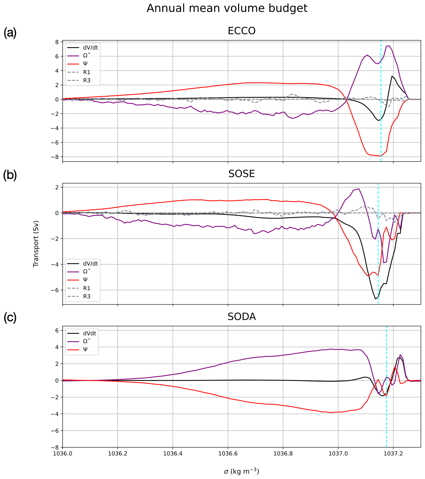
Figure 5 Main terms of the WMT volume budget in σ space (kg m⁻³) averaged over each model's respective time period for (a) ECCO (1992–2016), (b) SOSE (2006–2010) and (c) SODA (1993–2019). Volume change is represented by the black line and transport by the red line, transformation is the purple line (includes numerical mixing in ECCO and SOSE, and in SODA it also includes discretization residual), and the discretization residual is explicitly shown as the grey dashed line in ECCO and SOSE. The vertical dashed line demarcates the boundary of bottom water in each model (1037.155 kg m⁻³ for ECCO, 1037.145 for SOSE and 1037.175 kg m⁻3 for SODA).

Figure 6 (a) Transformation term, Ω (solid purple line), broken down into its sources of transformation: surface salt flux (orange dashed line), surface heat flux (blue dashed line) and mixing (slate-grey dashed line). Residual due to numerical mixing is the pink dashed line in ECCO (a) and SOSE (b). The vertical dashed line demarcates the boundary of bottom water in each model (1037.155 kg m⁻³ for ECCO, 1037.145 for SOSE and 1037.175 kg m⁻³ for SODA).

4 Climatological WMT budgets

4.1 Annual mean

We first examine the annual mean WMT budget, which represents the long-term mean transformation and overturning structure of the WG, averaging over all spatial and temporal variability. Figure 5a, b and c show the annual mean budget from ECCO, SOSE and SODA, respectively. The black line represents the time evolution of the cumulative water mass volume distribution, $\partial V/\partial t$, in the WG region during each model's respective time period. It is balanced by the total inflow/outflow transports (Ψ, red line) and mean transformation (Ω^∗, purple line), which includes the residual due to numerical mixing. Conceptual models usually assume that the system is in a steady-state balance between overturning and transformation ($\partial V/\partial t=\mathrm{0}$), but that is clearly not the case for any of the models examined here. The existence of a tendency indicates a model drift and/or low-frequency variability over the climatological period.

In σ₂ coordinates the water masses that are the Weddell Sea's recipe for AABW are distinguished as follows by their densities: CDW/WDW (Warm Deep Water) ($\mathrm{1037.13}<{\mathit{\sigma }}_{\mathrm{2}}<\mathrm{1037.24}$ kg m⁻³) and WSBW/HSSW/ISW (WSBW: Weddell Sea Bottom Water; ISW: Ice Shelf Water) (σ₂≥1037.2 kg m⁻³). Our budget coarsely separates all water into two classes, which are delineated by a boundary σ^†: bottom water (denser than σ^†) and deep water (by volume, mostly CDW and its regional variants). Due to volume conservation, in this construction, the transport of bottom water across the basin boundary is equal and opposite to the transport of deep water. The dividing isopycnal σ^† is defined for each model via the minimum of the overturning streamfunction (Ψ). Because the streamfunction is a cumulative integral quantity, the framework defines AABW transport as the flow across the boundary of all water denser than σ^†. So one single transport value represents both the deep outflow and the equal-and-opposite bottom water inflow. Recapitulating, here we define AABW's density (σ^†) specific to each model based on where each Ψ reaches its extreme (minimum value) after crossing 0. The values of σ^† are 1037.155 kg m⁻³ for ECCO, 1037.145 kg m⁻³ for SOSE and 1037.175 kg m⁻³ for SODA. On average, as shown by the negative extremum of Ψ, AABW is exported from the region at the rate of 7.9 Sv (Sv = 10⁶ m³ s⁻¹) in ECCO, 4.9 Sv in SOSE and 1.9 Sv in SODA. The export is countered by thermodynamic transformation (Ω) by 3.6 Sv in ECCO and 0.4 Sv in SODA and paired by Ω in SOSE by 1 Sv. This leads to a total volume loss of the bottom water class of 2.8 Sv in ECCO, 6.6 Sv in SOSE and 1.5 Sv in SODA. The export value from ECCO is similar to the mean outflow value of Kerr et al. (2012), who found the mean outflow of AABW to be 10.6±3.1 Sv using a $\mathrm{1}/\mathrm{12}$^∘ 20-year global ocean simulation. We note that though Kerr et al. (2012) obtained this value from a transect at the tip of the Antarctic Peninsula, they do attempt to capture the dominant outflow of the Weddell Sea AABW. Similar transport values of AABW have been reported by Talley et al. (2003), who determined 8.5 Sv of AABW traveling northward in the Atlantic sector of the Southern Ocean Meridional Overturning Circulation.

We now examine the thermodynamic processes driving transformation in more detail. AABW transformation in ECCO (Fig. 6a) is mainly due to brine rejection at the surface (orange dashed line). We categorize the transformation from surface salt fluxes as influence only from sea ice since our analysis showed an almost negligible role for the atmosphere. Therefore, positive transformation values are associated with brine rejection and negative values with ice melt. The effects of surface cooling and mixing are generally confined to lighter water masses in the region and tend to cancel each other out. However, mixing does have a stronger tendency to lighten bottom water (by about 4.5 Sv) than surface-cooling-induced positive transformation (0.6 Sv). In ECCO, the dominant impact of brine rejection on transformation (7.4 Sv) is similar to Iudicone et al. (2008a), who found brine rejection dominating the transformation of bottom water by ∼ 5 Sv. In SOSE (Fig. 6b) the effect of transformation on bottom water shows the opposite behavior to ECCO. SOSE's Ω is driven by mixing (2.8 Sv) and is countered by an equal combination of surface cooling and brine rejection (both 0.9 Sv). Overall, the ECCO and SOSE models are in qualitative agreement with the literature of what is known about bottom water circulation in the Weddell Sea (Carmack and Foster, 1975; Orsi et al., 1999; Meredith et al., 2000; Gordon et al., 2001; Naveira Garabato et al., 2002). The two models show that brine rejection and surface cooling drive positive bottom water transformation, while mixing with warmer WDW and fresher AAIW (Antarctic Intermediate Water) acts to decrease AABW. Because we cannot explicitly calculate WMT in SODA but rather infer it as a residual, it is not possible to further decompose SODA's transformation into different components.

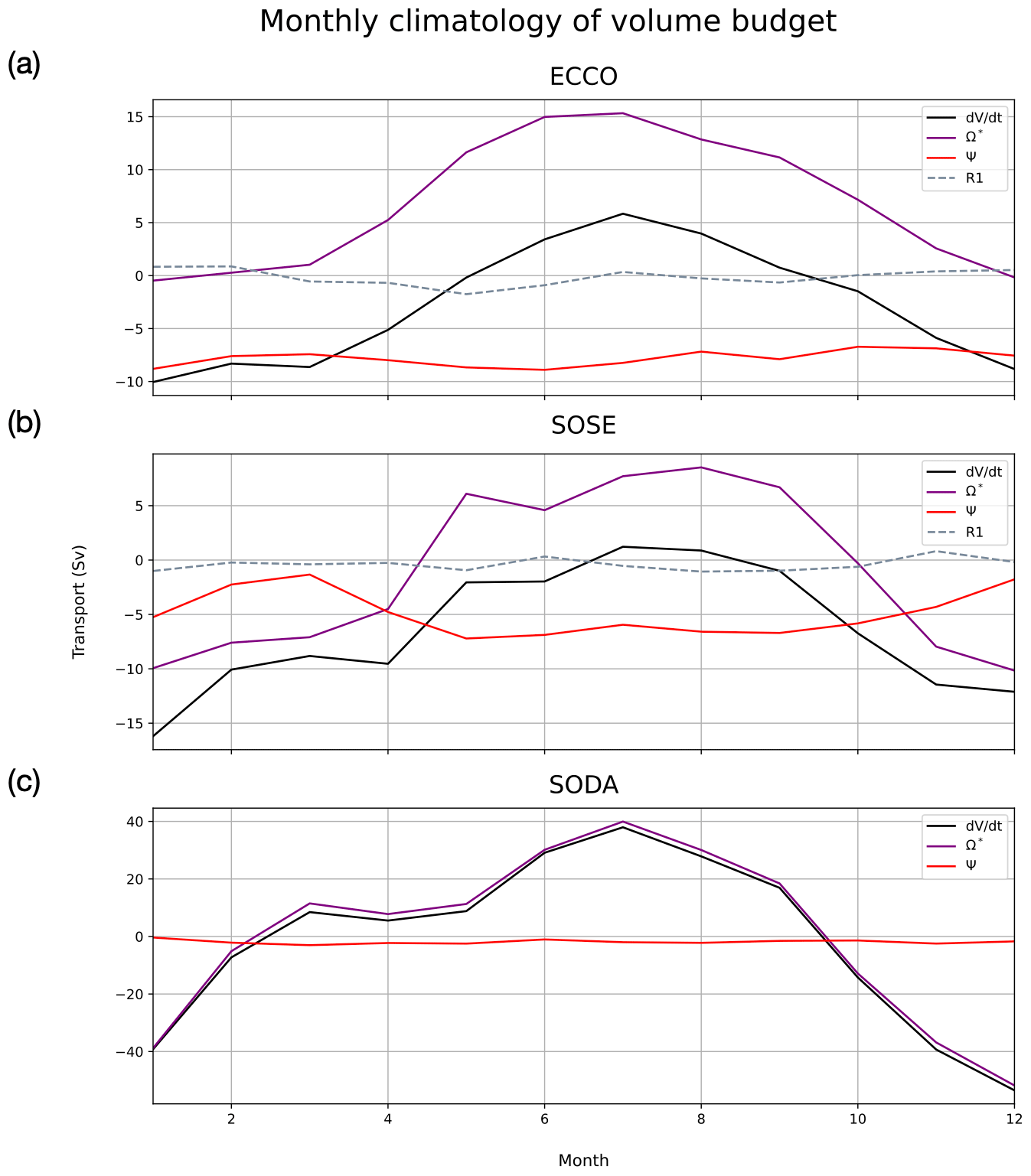
Figure 7 Monthly climatology of Weddell bottom water's main WMT budget terms in ECCO (a), SOSE (b) and SODA (c). Residual due to discretization (R1) only shown in ECCO and SOSE.

4.2 Seasonal climatology

While the long-term annual mean shown above is what matters most for the global-scale overturning and climate, the annual mean masks a huge amount of seasonality in WMT. Exploring this seasonality is important for understanding the mechanisms behind WMT. Here we examine the monthly climatology of the transformation budget in the three models (Figs. 7 and 8). The climatology of each term was calculated as a monthly average. Figure 8 shows this climatology via contour plot and for a wider range of densities to illustrate the seasonality across multiple water masses. For ECCO and SOSE, we also decomposed Ω into transformation from mixing, surface cooling/warming and surface freshwater fluxes in Fig. 9.

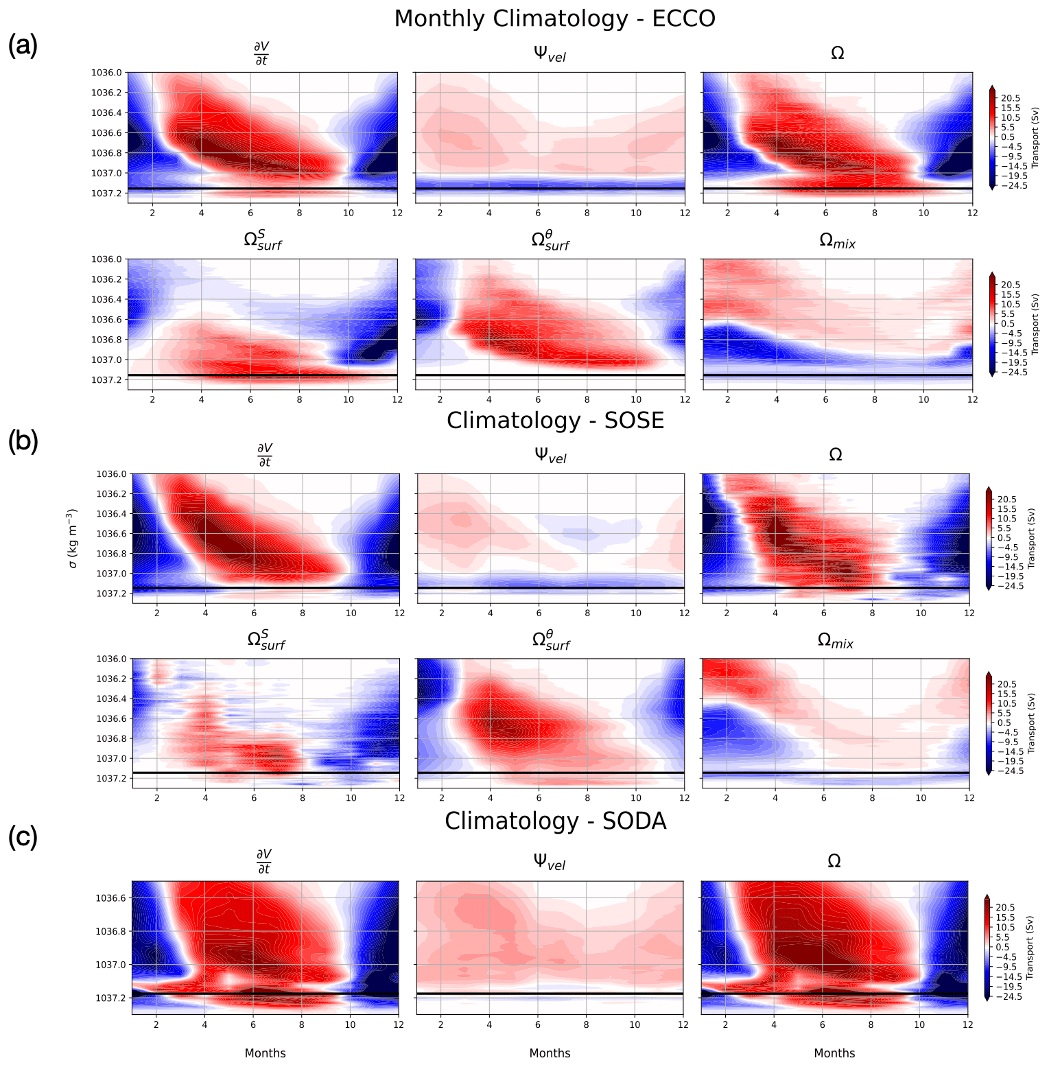
Figure 8 Monthly climatology of main WMT budget terms in top panels in ECCO (a), SOSE (b) and SODA (c) and sources of transformation (bottom panels) in ECCO (a) and SOSE (b). The horizontal black line represents the bottom water boundary in each model (1037.155 kg m⁻³ for ECCO, 1037.145 kg m⁻³ for SOSE and 1037.175 kg m⁻3 for SODA).

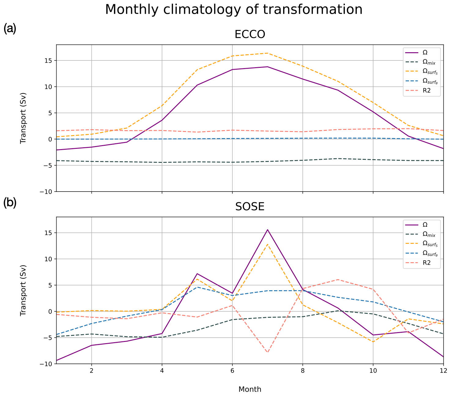
Figure 9 Monthly climatology of Weddell bottom water's transformation term (purple line) and its sources of transformation: surface salt flux (orange dashed line), surface heat flux (blue dashed line) and mixing (slate-grey dashed line). Residual due to numerical mixing is the pink dashed line in ECCO (a) and SOSE (b).

We switch to focus on a single time series that best represents AABW transformation and overturning, rather than the entire range of densities in Figs. 7 and 9. We do this by moving from a transformation budget to a formation budget. Again, for each model, we define the boundary between CDW (inflowing water) and AABW (outflowing water) as the density σ^† where Ψ reaches its extreme (minimum value). As stated before, the values of σ^† are 1037.155 kg m⁻³ for ECCO, 1037.145 kg m⁻³ for SOSE and 1037.175 kg m⁻³ for SODA. By sampling Ψ, Ω and $\partial V/\partial t$ at σ^†, we obtain a single value or time series representing the net export rate, formation rate and volume tendency of AABW.

In summary, the monthly view reveals that the overturning Ψ is relatively steady over the year in ECCO and SODA; in SOSE, transport shows more seasonality (Figs. 7 and 8). Next, Ω exhibits a seasonal cycle an order of magnitude larger than their annual mean. Moreover, the seasonal cycle in $\partial V/\partial t$ and Ω is largely compensatory; excess dense water is created by WMT in winter and then destroyed in summer, and a residual is left over for export from the basin via Ψ. However, in ECCO the destruction is caused by less contribution from transformation and the influence of outflow becomes compensatory.

Going into more detail with Fig. 7, we see from all three models that bottom water gains volume during the austral winter months and loses volume during the rest of the year. However, in SODA (Fig. 7c), bottom water volume gain occurs over a longer time range: for three-quarters of the year. SOSE reveals a slight imbalance between the formation rate of AABW and its export; more water is being exported over the year than is being formed. This leads to a continuous decrease in AABW volume, which we will see is the case in Sect. 5 (also visible in Fig. 5b). However, superimposed upon this overall trend is a strong seasonal cycle, with excess AABW production and a corresponding volume tendency in winter.

One immediately notices in SODA (Fig. 7c) the overall larger monthly variability. There was also a dramatic switch between volume gain in January to significant volume loss in February (>25 Sv). SODA, as it was detailed in Sect. 3.4, differs from the other two data-assimilating models in that SODA nudges the data to fit the observations it is trying to match. Such a data-assimilating technique commonly causes jumps in the data and produces unphysically large magnitudes in our budget terms, which is consequently evident in our water mass transformation budgets. For this reason, we inserted averaged salt and temperature values from the day before and day after some of the spikes we observed in our preliminary analyses. It would help to remind the reader that the Ω^* term shown here is not quite the same as the transformation terms shown for ECCO and SOSE. The transformation term in SODA implicitly carries the residuals that were explicitly calculated in ECCO and SOSE (R1 and R2). In SODA, the advective transport of bottom water is almost insignificant compared to the large magnitude of inferred transformation. SODA still concurs with ECCO and SOSE in showing that volume gain occurs during the winter months; however, bottom water volume grows over half a year as opposed to only a few months centered in the year in ECCO and SOSE.

Looking at $\partial V/\partial t$ over a wider density range in Fig. 8, we can see in all three models that densification acts upon the lighter densities at the beginning of winter, and as the season progresses the thermodynamic process moves down to transform the denser range of the ocean. This pattern can be derived from the surface cooling component of transformation in ECCO and SOSE. This is in agreement with the general understanding that AABW in the Weddell Sea is created when sea ice forms during the winter season, and during the warmer months the production of AABW decreases (Fig. 7a) or is even destroyed (Fig. 7b and c). There is year-round export of bottom water in all three models, with the intensity of outflow peaking and varying in the middle of the year. Peak export happens at ∼10 Sv in June in ECCO, ∼12 Sv April–July in SOSE and ∼3 Sv in March in SODA. Both ECCO and SOSE values are within the error bars of the Kerr et al. (2012) maximum monthly mean outflow value of 12.2±3.0 Sv.

Breaking down the components of Ω (Fig. 9), we can see some significant differences between ECCO and SOSE; however, note how both models exhibit a broadly similar σ-temporal structure in these terms (Fig. 8a and b) but with a different magnitude and position within σ space. In ECCO (Fig. 9a), the contribution of ${\mathrm{\Omega }}_{\mathrm{surf}}^{\mathit{\theta }}$ is negligible, and ${\mathrm{\Omega }}_{\mathrm{surf}}^{\mathrm{S}}$ is positive throughout the winter; this indicates that brine rejection is the dominant process behind AABW formation, as was seen in the annual mean budget (Fig. 6a), with little impact from ice melt, runoff or precipitation. All the while, throughout the year, transformation due to mixing is trying to homogenize the waters; therefore, bottom water is essentially being destroyed throughout the year on the order of 4 Sv.

In SOSE (Fig. 9b), AABW production during the winter months is also mainly due to brine rejection. Unlike ECCO, surface cooling provides an additional source for AABW formation in SOSE. Mixing, though more variable throughout the year in SOSE than in ECCO, still works to homogenize (destroy) bottom water. Towards the end of the winter season, ${\mathrm{\Omega }}_{\mathrm{surf}}^{\mathrm{S}}$ is negative, corresponding to ice melt.

5 Interannual variability

Having examined the climatology, we now turn to the main focus of our study: quantifying the interannual variability of AABW production in these reanalyses. A deep look at the interannual variability of the anomalous WMT budget terms reveals some interesting differences in AABW circulation between these three models and also serves as a point of comparison with similar studies (Iudicone et al., 2008a, b; Abernathey et al., 2016; Gordon et al., 2020). In this section, we highlight some anomalous events and the differences between all three models.

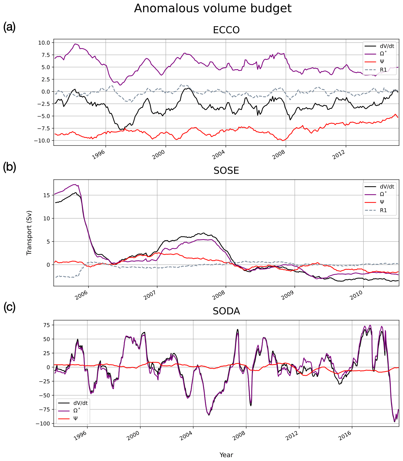
Figure 10 Anomalous main terms of WMT volume budget in ECCO (a), SOSE (b) and SODA (c). Time series was smoothed by an annual rolling mean with the center window set to the middle of the year. Volume change is the black line and transport the red line, transformation is the purple line (includes R2 in ECCO and SOSE, and in SODA it also includes R1 and R2), and the discretization residual is explicitly shown as the dashed grey line in ECCO and SOSE.

Figure 11 Anomalous transformation term, Ω (solid purple line), broken down into its sources of transformation: surface salt flux (orange dashed line), surface heat flux (blue dashed line) and mixing (slate-grey dashed line). R2 is the pink dashed line.

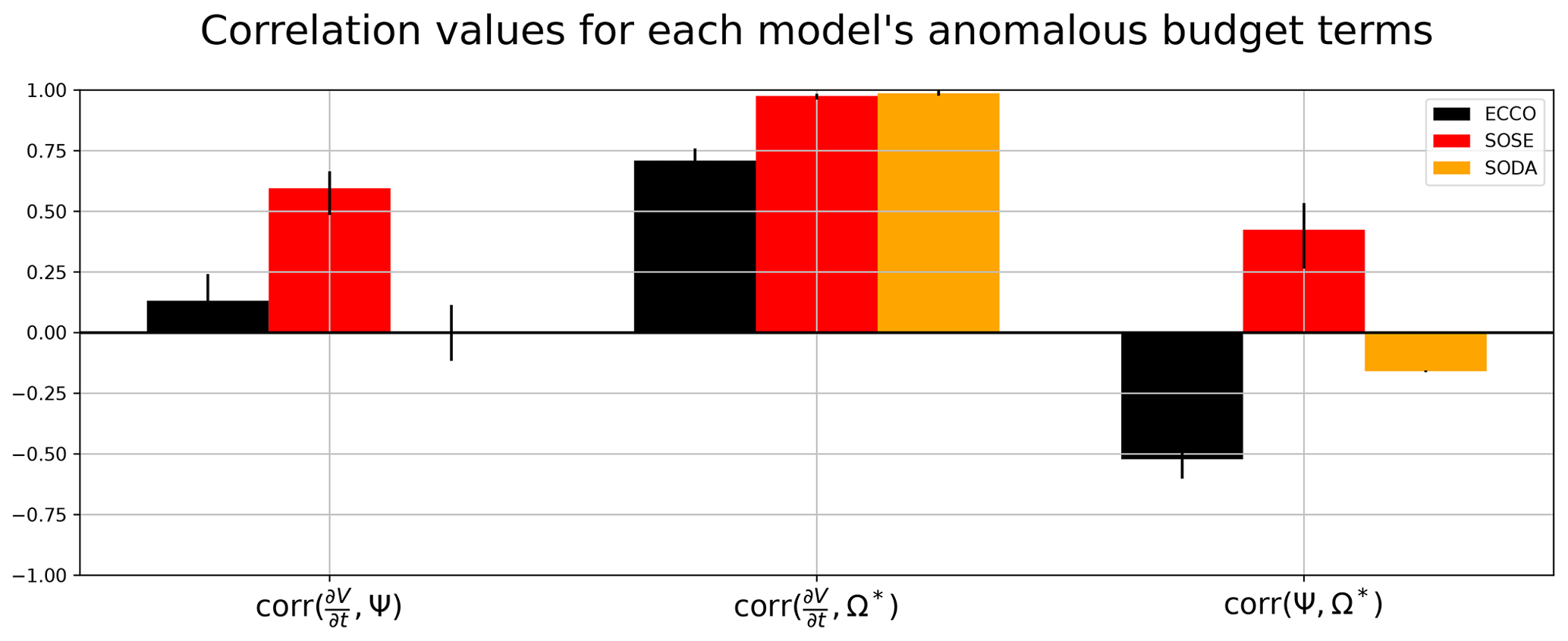
Figure 12 Correlation (and associated error bars) between the main budget terms from each model. The bars in black represent the correlation values in ECCO, red bars those in SOSE and orange bars those in SODA.

The anomaly time series for each model are constructed by sampling Ψ, Ω and $\partial V/\partial t$ at σ^† and then removing the monthly climatology for each term, and they are smoothed by a rolling mean with the center window set to the middle of the year; they are shown in Fig. 10. For ECCO and SOSE, we also decompose Ω into components due to surface heating, surface salt flux and interior mixing in Fig. 11. Figures 10 and 11 are thus completely analogous to Figs. 7 and 9 but for the interannual variability rather than the seasonal cycle. The anomaly WMT time series each cover a different time period. SODA is the longest and provides the most recent data; the data we extracted begin in 1993 and go through 2020. ECCO begins in 1992 and extends through 2016. SOSE's time period is the shortest out of the three models; while it is the highest-resolution product analyzed here, its 6-year period offers only a very limited view of interannual variability.

The most immediate feature that jumps out from Fig. 10 is the fact that the magnitude of the variability of $\partial V/\partial t$ in SODA is nearly 10× larger than ECCO and SOSE, with values as large as 75 Sv. This indicates that the volume of AABW in SODA is changing by huge amounts from year to year. These changes are not explainable by variations in overturning Ψ, so they must be balanced by the inferred WMT Ω^∗ (recall that we cannot diagnose Ω directly from SODA but instead infer it as a residual). We hypothesize that these large-magnitude changes in AABW volume are due to SODA's data assimilation nudging the temperature and salinity fields, without a driving physical process.

The ECCO time series (Fig. 10a) reveal some degree of variability (approx. 2–4 Sv) in the WMT budget; but there is also an overall consistent relationship between terms, with anomalous transformation always positive and transport always negative. The trend in AABW variability seems to be driven mainly by transformation, but its effects are constantly countered by export. In other words, the more AABW that is being formed in certain years (e.g.,  1999, 2001 and 2007) the more is being exported.

Digging into the decomposition of WMT terms in ECCO (Fig. 11a), we see, somewhat unsurprisingly, that WMT variability is largely driven by variability in surface salt fluxes. These trends are challenged by a considerable amount of mixing. The one exception to the dominant activity of surface salt fluxes in transformation is an event occurring from 2004–2008, which is associated with anomalously strong surface cooling (surface heat fluxes are otherwise negligible in the AABW budget for ECCO). Our initial assumption during this 2004–2008 period was that a polynya occurred, as is the case for SOSE in 2005. However, surface heat flux and sea ice cover maps with overlaid ${\mathit{\sigma }}_{\mathrm{2}}^{†}$ contours (not shown here) show no evidence of a simulated polynya but do show outcropping of the AABW contour in the open region of the Weddell Sea. We also considered the possibility of a polynya with thin ice coverage. Setting the sea ice thickness threshold to be 12 cm (consistent with Nakata et al., 2021, and Mohrmann et al., 2021), we still found no link between polynya and the AABW outcropping. We suspect that internal dynamics in ECCO drive AABW to outcrop under sea ice, where it loses heat. The heat loss due to this interaction is largely compensated for by heat gain due to mixing, likely associated with convective mixing in the outcrop region.

SOSE is unique among the three models in showing a persistent trend in the WMT budget over its (relatively short) time period. As shown earlier in Fig. 5b, SOSE is losing AABW and gaining CDW at a rate of ∼ 10 Sv over this time period, which is mainly driven by trends in decreasing formation and ultimately increasing destruction of AABW after 2008. In the anomaly time series (Fig. 10b), we see that this trend is not steady but in fact accelerates over time. Production of AABW (Ω) is anomalously strong at the beginning of the state estimate (2005) and decreases by 16 Sv by 2010. Figure 11b shows that this decrease in production rate is driven primarily by trends in mixing and secondly by trends in surface cooling. Surface salt fluxes do little to counter these effects. In the first year of the state estimate, an open-ocean polynya event contributes to enhancing the production of AABW via surface heat fluxes; after that, there is negligible anomalous surface-heat-flux-driven production. There is some variability in production from surface salt fluxes of the order of 1–2 Sv. During late 2006 to 2008, transport of AABW (Ψ) helps to increase volume distribution by ∼ 3 Sv (note that Fig. 10 shows the anomaly relative to the climatology, not the absolute value). After that, the residual imbalance between Ψ and Ω drives an acceleration in the rate of volume loss of AABW. Overall, SOSE is the farthest of all the models from a state of balance between production and export of AABW.

In general, the time series in Fig. 10 contain many different relationships between the different budget terms in different models. To try to summarize these relationships, we compute correlations between each pair of terms. These correlations quantify the extent to which one term balances the other in a budget (Tesdal and Abernathey, 2021); for example, a correlation of 1 between $\partial V/\partial t$ and Ω means that trends in volume distribution are completely driven by anomalous water mass transformation. All reported correlation coefficients are statistically significant with a confidence level of 95 %. For ECCO (black bars in Fig. 12), $\partial V/\partial t$ is weakly correlated with transport Ψ (0.13; p value = 3 × 10⁻²; confidence interval of 0.01 and 0.25) and strongly correlated with transformation (0.71; p value = 2 × 10⁻⁴³; confidence interval of 0.65 and 0.76), indicating a dominant compensation of transformation on $\partial V/\partial t$. The correlation between Ψ and Ω is negative (−0.52; p value = 1 × 10⁻²⁰; confidence interval of −0.60 and −0.43). In SOSE (red bars), there is a positive correlation between transformation and transport (0.70; p value = 2 × 10⁻⁹; confidence interval of 0.54 and 0.82). Similar to ECCO, there is a stronger relationship between trends in volume and transformation (0.98; p value = 2 × 10⁻³⁸; confidence interval of 0.96 and 0.99) relative to transport (0.82; p value = 1 × 10⁻¹⁴; confidence interval of 0.71 and 0.89); in SOSE, volume trends in AABW are driven by variability in both transformation and transport. Finally, in SODA (orange bars), variability is completely driven by transformation (0.99; p value = 1 × 10⁻²⁰¹; confidence interval of 0.98 and 0.99) and has no relationship to transport (0; p value = 3 × 10⁻³; confidence interval of 0 and 0.06). There is a weak anti-correlation between transport and transformation (−0.16; p value = 1; confidence interval of −0.12 and 0.12). Overall, the correlation analysis confirms what is seen visually in the time series; each reanalysis has a different overall relationship between WMT budget terms, yet they all show a positive and stronger relationship between $\partial V/\partial t$ and Ω than between $\partial V/\partial t$ and Ψ.

Many studies have argued for links between large-scale climate indices and AABW production/export (Gordon et al., 2007; Meredith et al., 2008; Gordon et al., 2010; McKee et al., 2011; Gordon et al., 2020). We examined this in the three reanalyses by calculating correlations between the terms in the WMT budgets and climate forcings from the El Niño–Southern Oscillation (ENSO), the Southern Annular Mode (SAM), wind stress curl (WSC) and sea ice concentration (SIC). ENSO data were taken from the NOAA Extended Reconstructed Sea Surface Temperature (ERSST) version 5 project (Huang et al., 2017). The SAM index was obtained from Marshall and National Center for Atmospheric Research Staff (2021). Wind stress curl was calculated from ERA-Interim zonal wind stress state variables (Dee et al., 2011), and, finally, for sea ice concentration we used each model's sea ice concentration diagnostic averaged over the WG region. We standardized each index by dividing the anomaly time series by their respective standard deviation in time. Notable correlation values in SOSE are between all the budget terms and SIC: $\partial V/\partial t$ and SIC (−0.60; p value = 1 × 10⁻⁶; confidence interval of −0.74 and −0.40), Ψ and SIC (−0.70; p value = 5 × 10⁻⁹; confidence interval of −0.81 and −0.52), and Ω and SIC (−0.53; p value =  3 × 10⁻⁵; confidence interval of −0.70 and −0.31). Additionally, observed between all three budget terms and WSC were positive correlations: $\partial V/\partial t$ and SIC (0.33; p value = 1 × 10⁻²; confidence interval of 0.07 and 0.55), Ψ and SIC (0.34; p value = 1 × 10⁻²; confidence interval of 0.08 and 0.55), and Ω and SIC (0.33; p value = 2 × 10⁻²; confidence interval of 0.07 and 0.54). In SODA, transport is negatively correlated with SIC (−0.46; p value = 2 × 10⁻¹⁵; confidence interval of −0.55 and −0.36). In ECCO, there were no notable correlations between budget terms and climate indices.

6 Discussion and conclusion

Overall, the main contribution of our study is to diagnose, for the first time, a closed, time-dependent water mass budget for AABW in the Weddell Sea from three state-of-the-art ocean reanalyses. This gives an unprecedented view of the processes that control the volume, production and export of AABW from this climatically important region. In the long-term annual mean, all three models produce and export AABW at rates broadly compatible with observations. However, there is little agreement between these reanalysis products on interannual timescales.

We now summarize some of the main features of the AABW volume budget time series in each reanalysis. SODA showed an extreme amount of variability in AABW volume in the WG which could not be explained by variations in export. Although we could not diagnose WMT explicitly in SODA due to its lack of closed heat and salt budgets, the only possible explanation for this variability is WMT, likely driven by the nudging tendencies of the data assimilation scheme. The obvious conclusion is that reanalyses based on 3DVar data assimilation are not suitable for WMT studies since they are not constrained to actually conserve heat and salt. Due to their adjoint-based data assimilation, ECCO and SOSE do provide such closed budgets and can therefore provide better insight into the drivers of variability in WMT. Both models show strong interannual variability in the AABW volume budget. SOSE's short time period makes it hard to draw general conclusions; during this time period there is an accelerating loss of AABW, driven largely by interior mixing and changes in surface salt fluxes. The transformation changes are paired with a weaker influence from export. Given the short time period of SOSE, these trends may simply be a part of low-frequency interannual variability. Indeed ECCO does display such interannual variability; there are numerous 5-year periods that show secular trends in one or more terms. Moreover, there is some indication of alignment in these trends between ECCO and SOSE, particularly the strong decline in AABW production from 2007–2010. In our assessment, ECCO provides the most useful time series for revealing the processes and mechanisms that drive WMT and export variability. It exhibits interannual fluctuations offset by its mean state with a reasonable magnitude relative to the climatology. The decomposition of WMT in ECCO reveals a rich interplay between variability in export, surface forcing and interior mixing in driving AABW volume variability.

Because of the difficulty of observing the deep outflow of AABW, it would be very useful if we could relate AABW export to surface processes in the Weddell Sea. Gordon et al. (2020) showed strong interannual variability in Weddell Sea Bottom Water salinity, as measured by nearly 20 years of mooring data in the northwest Weddell basin. They made the case that this variability was tied to the strength of the WG and ultimately the wind stress curl, which is influenced by large-scale climate modes such as ENSO and SAM. In a similar vein, Kerr et al. (2012) found a strong co-varying relationship between bottom water transport and brine rejection in a 20-year high-resolution numerical simulation. We searched for such relationships in ECCO and SOSE. We found transport in SOSE to be strongly correlated with surface-salt-flux-induced transformation (0.66; p value =  4 × 10⁻⁸; confidence interval of 0.48 and 0.79) and weakly correlated with surface-heat-flux-induced transformation (0.28; p value =  4 × 10⁻²; confidence interval of 0.02 and 0.51) as well as with mixing-induced transformation (0.27; p value = 4 × 10⁻²; confidence interval of 0.01 and 0.50). Both this study and Kerr et al. (2012) find that salt fluxes near the surface and bottom water export co-vary as they are both directly influenced by wind forcings that influence WG strength. We found the wind stress curl over the WG region to be most correlated with the surface salt flux source of transformation, though the relationship is indeed weak (0.28; p value = 4 × 10⁻²; confidence interval of 0.02 and 0.51) in SOSE. However, SOSE is very short, so these correlations are not definitive. In contrast, the only notable relationship between transport and the different sources of transformation in ECCO was between Ψ and surface-salt-flux-induced transformation (−0.44; p value = 3 × 10⁻¹⁴; confidence interval of −0.53 and −0.34). We note the importance of the volume tendency term $\partial V/\partial t$ in the WMT budget. When this term is large, it means that excess AABW production need not correspond to export; instead, it can drive large trends in the water mass distribution within the basin, without any impact on export. Over its 25-year time series, the relationship between the terms in the WMT budget changes dynamically, with no clear dominant balance. This complexity confounds the goal of establishing a simple relationship between surface forcing and AABW export. This is an important insight for studies of the WG based on surface and satellite-based observations.

Numerous studies have shown that AABW in the Weddell Sea has been warming (Robertson et al., 2002; Fahrbach et al., 2004; Purkey and Johnson, 2010; Fahrbach et al., 2011; Meredith et al., 2011; Couldrey et al., 2013), freshening (Jullion et al., 2013) and losing volume (Purkey and Johnson, 2012; Kerr et al., 2018). Purkey and Johnson (2012) suggest that the decline in AABW production by a rate of −8.2 (±2.6 Sv) is the cause of the contraction of bottom water volume for the period 1993–2006. As shown in the annual mean (Fig. 5), all three models are losing AABW volume, with SOSE losing AABW much faster. In all three models, the decline in AABW is due to an imbalance between AABW formation and export: the models export more AABW than they produce. In ECCO, the volume loss is roughly steady over 25 years, with significant interannual variability. In SOSE, in contrast, it accelerates strongly over the 6-year period.

In Hellmer et al. (2011), it is hypothesized that the freshening of the northwest shelf water contributing to an increase in glacial meltwater input is the cause of the slowdown of AABW production rate. Surface freshening makes it more difficult for surface and shelf waters to sink, which slows the production of AABW and, subsequently, the circulation of the lower limb of the MOC. In SOSE (Fig. 11b), there is a declining trend in transformation, partly due to a switch from brine-rejection-inducing formation prior to mid-2008 to freshwater input, causing AABW destruction from 2008 to mid-2009 and staying roughly near 0 thereafter. Since SOSE does not include time-variable runoff, such trends must be due to variations in sea ice. In ECCO, we do not see such a trend in transformation or in freshwater-flux-sourced transformation to suggest a decline in AABW volume due to freshening.

Our project has sought to explore how current state-of-the-art data-assimilating ocean reanalyses can help fill the gaps in our understanding of the thermodynamic drivers of AABW export variability from the Weddell Sea, specifically, the quantitative links between surface forcing, interior dynamic and thermodynamic processes, and outflow. From the WMT analysis employed with the three ocean state estimates, we have determined that the variability of AABW is driven by a combination of surface forcings derived from strong winds and brine rejection and interior diapycnal mixing. An additional initial goal of our work was to probe the mechanistic link between climate forcings, SAM and ENSO, and AABW transformation and export, as has been suggested by observations (Gordon et al., 2020). However, none of the reanalyses we analyzed exhibited such clear links. We had further hoped that, since these reanalyses assimilate data and aim to capture the real history of the ocean state, they might simulate the specific phasing of interannual variability seen in the mooring records (Gordon et al., 2020); however, this was not the case. The discrepancies between the models and between the models and observations suggest that this class of reanalysis is not capable of consistently and faithfully capturing the processes that drive AABW variability in a robust way. Similar to the conclusions of Heuzé et al. (2013) and Heuzé (2021) regarding CMIP5 and CMIP6 models, respectively, the relatively coarse resolution of these models makes it difficult to resolve processes such as coastal polynyas, dense overflows and the sharp, v-shaped front of the western boundary current which Gordon et al. (2020) argued was crucial for the pathway of AABW export.

Regardless of these shortcomings, we feel that the time-dependent water mass framework presented here is a useful tool for understanding AABW variability in this region. A very promising direction for future work would be to apply the same methodology to higher-resolution models, which presumably represent small-scale processes with much greater fidelity. A recent study by Stewart (2021) showed that a $\mathrm{1}/\mathrm{12}$^∘ regional model of the Weddell Sea could resolve the impact of tides and eddies on cross-shelf transfer of buoyancy, resulting in a more realistic overturning circulation. High-resolution global ocean climate models (e.g., Small et al., 2014; Morrison et al., 2016; Kiss et al., 2020) are also capable of resolving these processes in better detail and would be a promising tool for investigating AABW WMT. One challenge, however, in applying the WMT approach to these models is the computationally demanding nature of the WMT diagnostics, which require closed heat and salt budgets to begin with and then layer on additional complex calculations.

We also note the limitations of the potential-density WMT framework used here. Our method is not capable of explicitly diagnosing WMT effects due to the nonlinear equation of state (cabbeling and thermobaricity); even those processes are hypothesized to be important for the transformation of water masses into AABW (Gill, 1973; Gordon et al., 2020; Mohrmann et al., 2022). Alternative frameworks use neutral density (Jackett and McDougall, 1997; Iudicone et al., 2008b) or move to two-dimensional temperature/salinity water mass coordinates (Evans et al., 2018), which can reveal subtleties in the transformation process that are inaccessible to the 1-D density-based approach. We look forward to exploring these possibilities in future work.