A numerical investigation on the energetics of a current along an ice-covered continental slope

The Chukchi Slope Current is a westward-flowing current along the Chukchi slope, which carries Pacific-origin water from the Chukchi shelf into the Canada Basin and helps set the regional hydrographic structure and ecosystem. Using a set of experiments with an idealized primitive equation numerical model, we investigate the energetics of the slope current during the ice-covered period. Numerical calculations show that the growth of surface eddies is suppressed by the ice friction, while perturbations at mid-depths can grow into eddies, consistent with linear instability analysis. However, because the ice stress is spatially variable, it is able to drive Ekman pumping to decrease the available potential energy (APE) and kinetic energy of both the mean flow and mesoscale eddies over a vertical scale of 100 m, well outside the frictional Ekman layer. The rate at which the APE changes is determined by the vertical density flux, which is negative as the ice-induced Ekman pumping advects lighter (denser) water upward (downward). A scaling analysis shows that Ekman pumping will dominate the release of APE for large-scale flows, but the effect of baroclinic instability is also important when the horizontal scale of the mean flow is the baroclinic deformation radius and the eddy velocity is comparable to the mean flow velocity. Our numerical results highlight the importance of ice friction in the energetics of the slope current and eddies, and this may be relevant to other ice-covered regions.

1 Introduction

Continental slopes of Arctic shelf seas usually feature strong boundary currents, which transport water and nutrients and play a crucial role in shaping the Arctic ecosystem (Bluhm et al., 2020; Oziel et al., 2022). In the western Arctic Ocean, the Chukchi continental slope is known to be the main passage for the Pacific-origin water after it exits the Chukchi shelf through Barrow Canyon (e.g., Corlett and Pickart, 2017; Li et al., 2019; Stabeno and McCabe, 2020) (see the schematic circulation in Fig. 1). The westward-flowing current along the Chukchi slope, named the Chukchi Slope Current (CSC) (Corlett and Pickart, 2017), is suggested to be distinct from the southern arm of the Beaufort Gyre (BG) due to their different origins (Watanabe et al., 2017; Spall et al., 2018). Onshore of the slope current is the bottom-intensified, eastward-flowing Chukchi Shelf-break Jet (Corlett and Pickart, 2017; Li et al., 2019). In addition, there is an eastward-flowing current overlying the mid-slope of the Chukchi Sea, known as the inshore branch of the Atlantic Water Boundary Current (Corlett and Pickart, 2017; Stabeno and McCabe, 2020; Li et al., 2020).

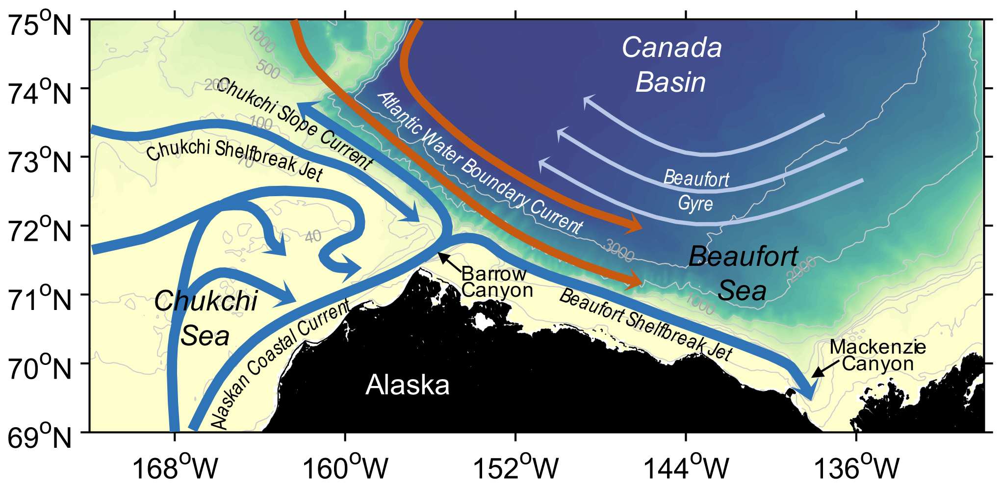
Figure 1 Schematic circulation in the Chukchi and Beaufort Seas; from Leng et al. (2022).

A year-long mooring array shows that the CSC is surface-intensified in summer and fall, but it becomes subsurface-intensified during winter and spring (Li et al., 2019). This is also supported by the results from a pan-Arctic numerical model (Leng et al., 2021). Using a simplified quasi-geostrophic theoretical model, Leng et al. (2022) further demonstrated that the structure of the CSC is related to the ice condition. Typically, the slope current is laterally sheared, and the corresponding spatially variable friction between the ice and the slope current can drive an overturning circulation to modify the thermal wind shear. This then results in the formation of a subsurface velocity maximum (via geostrophic setup) as seen in the mooring observations (Li et al., 2019).

It is well established that the “ice–ocean governor” – the negative feedback between the ice and ocean currents – acts to help equilibrate the BG by diminishing the wind-driven Ekman pumping (e.g., Meneghello et al., 2018, 2020; Dewey et al., 2018; Zhong et al., 2018; Doddridge et al., 2019). In addition, the ice friction can suppress surface instabilities (Meneghello et al., 2021) and dissipate existing surface eddies (Ou and Gordon, 1986), and this helps to explain the observed subsurface kinetic energy (KE) maxima in the interior Canada Basin. A recent idealized numerical study suggests that the dissipation of surface eddies relies heavily on the sea ice concentration (Shrestha and Manucharyan, 2022). When the sea ice concentration is high enough, the ice cover acts as a nearly immobile surface lid and thus dissipates the surface eddies effectively.

The Chukchi continental slope is one of the most energetic regions in the western Arctic Ocean as it is populated with strong boundary currents and mesoscale eddies (Kubryakov et al., 2021; Wang et al., 2020). These eddies, either formed via local baroclinic instability or propagated from other areas, are important in the exchanges of water masses and energy between the CSC and BG. During summer months, the CSC appears as a meandering free jet with opposing cross-stream gradients of potential vorticity (PV) within the current – a necessary condition for baroclinic instability (Corlett and Pickart, 2017). However, it is not yet clear whether the CSC is baroclinically unstable during the ice-covered period and how the ice friction works on the energetics of the current and eddies.

In this paper, we investigate the slope current energetics using a set of experiments with an idealized primitive equation numerical model. Our focus is on the period when the slope region is covered by packed ice with a 100 % concentration rather than the full melting–freezing cycle. Section 2 describes the model configuration and outlines the procedures for the energetics calculations and linear instability analysis. Section 3 shows results from the base and sensitivity experiments and illuminates the role of ice friction in the slope current energetics. Finally, a summary and discussion are given in Sect. 4.

2 Methods

2.1 Model description

The Massachusetts Institute of Technology general circulation model (MITgcm) (Marshall et al., 1997) is used in this study. A meridional channel bounded by two solid walls is set up on a 300 km (width) by 200 km (length) Cartesian grid with an application of periodic boundary conditions at the northern and southern edges (see the schematic in Fig. 2). For discussion purposes axes x, y, and z denote cross-channel, along-channel, and upward directions, respectively. The topography is idealized for a continental shelf (x=0 to 50 km, $z=-\mathrm{100}$ m), slope (x=50 to 90 km, slope = 0.01), and open ocean (x=90 to 300 km, $z=-\mathrm{500}$ m). The horizontal resolution is 1 km so that mesoscale eddies (with a typical length scale of 10 km) can be resolved. There are 48 levels in the vertical with the layer thickness increasing from 2 m at the surface layer to 25 m at the bottom layer. The Coriolis parameter is constant: $f=\mathrm{1.4}\times {\mathrm{10}}^{-\mathrm{4}}$ s⁻¹.

Figure 2 Schematic of the model domain and bottom topography. The initial current flows northward along the channel with its onshore part overlying the continental slope.

Parameterizations for this idealized model follow a pan-Arctic model that has been used to study the origin and fate of the CSC (Leng et al., 2021). The ocean model utilizes a nonlinear equation of state of seawater (Jackett and McDougall, 1995). Vertical mixing is calculated by the nonlocal K-Profile Parameterization (KPP) mixing scheme (Large et al., 1994). The KPP background diffusivity is small ($\mathrm{5.44}\times {\mathrm{10}}^{-\mathrm{7}}$ m² s⁻¹) as required by the parameterization of a salt plume (Nguyen et al., 2009). The modified horizontal viscosity scheme of Leith (1996) that can sense the flow divergence (Fox-Kemper and Menemenlis, 2008) is used with nondimensional Leith biharmonic viscosity factor 1.5. We also set a quadratic bottom drag with coefficient $\mathrm{2.0}\times {\mathrm{10}}^{-\mathrm{3}}$ and free-slip lateral boundary conditions. The viscous–plastic dynamic–thermodynamic sea ice model of Zhang and Hibler (1997), as modified by Losch et al. (2010), is coupled to the ocean model.

The model is initialized with a northward-flowing geostrophic current with its onshore part overlying the continental slope (Fig. 2). This is similar to the CSC flowing along the Chukchi slope (Corlett and Pickart, 2017). The initial along-channel velocity is given by (Fig. 3a)

$$\begin{array}{}\text{(1)}& v^{\mathrm{ini}}\left(x,z\right)=\left\{\begin{array}{l}\frac{V_{\mathrm{m}}}{\mathrm{2}}\left[\cos \left(\frac{\mathit{\pi }z}{\mathrm{300}}\right)+\mathrm{1}\right]\sin \left[\frac{\mathit{\pi }\left(x-\mathrm{65}\right)}{L_{\mathrm{0}}}\right],\\ \mathrm{65}\le x\le \mathrm{115}\mathrm{km},-\mathrm{300}\le z\le \mathrm{0}\mathrm{m},\\ \mathrm{0},\mathrm{elsewhere},\end{array}\right.\end{array}$$

where V_m=0.2 m s⁻¹ is the maximum velocity and L₀=50 km is the flow width. The initial potential density field ρⁱⁿⁱ (Fig. 3a, black contours) is derived from the velocity field with consideration of the thermal wind relation, $f_{\mathrm{0}}(\partial v^{\mathrm{ini}}/\partial z)=-(g/{\mathit{\rho }}_{\mathrm{0}})(\partial {\mathit{\rho }}^{\mathrm{ini}}/\partial x$), where g=9.8 m s⁻² is the gravitational acceleration and ρ₀=1028 kg m⁻³ is the reference density. The density profile at the flow center (x=90 km) (Fig. 3c, red curve) is calculated from the December monthly mean salinity and temperature profiles at 72.625^∘ N, 156.875^∘ W (Fig. 3d), which are taken from the World Ocean Atlas climatology for the period 2005–2017 (Zweng et al., 2019; Locarnini et al., 2019). The constructed density field shows a similar vertical structure as in the shipboard observations (see Fig. 4 in Corlett and Pickart, 2017). The initial salinity field Sⁱⁿⁱ input to the model is derived from the density field by assuming ∇ρⁱⁿⁱ=β∇Sⁱⁿⁱ, where ∇ is the gradient operator and β=0.8 kg m⁻³ psu⁻¹ (note that temperature has little impact on density at near-freezing temperatures). We also input an initial temperature field Tⁱⁿⁱ which satisfies $\mathrm{\nabla }{T}^{\mathrm{ini}}\times \mathrm{\nabla }{S}^{\mathrm{ini}}=\mathrm{0}$; i.e., the initial temperature is distributed following the isohalines (or isopycnals) (Fig. 3b). Using the constructed density field, we calculate the background mean stratification $N^{\mathrm{2}}=-(g/{\mathit{\rho }}_{\mathrm{0}})(\partial {\mathit{\rho }}_r/\partial z$), where ρ_r is the area-mean potential density as a function of depth. The resulting stratification reveals two peaks in the vertical, the shallower peak at a depth of −59 m and the deeper peak at −218 m (Fig. 3e). A similar double-peak feature is also shown in the stratification profiles computed from the hydrographic and mooring data in the interior Canada Basin (Meneghello et al., 2021).

The deformation radius in the continuously stratified ocean can be estimated by $L_D=NH/f$, where H is the vertical scale of the mean stratification. In our model, with N=O(10⁻² s⁻¹) and H=O(100 m), L_D is about 10 km, which is identical to the length scale of the fast-growing halocline mode from instability analysis and also the halocline eddies in our simulations (see the details in Sect. 3). This is also similar to the first baroclinic deformation radius in the Arctic Ocean, which ranges from ∼ 5 km in the Nansen Basin to ∼ 15 km in the central Canada Basin (Nurser and Bacon, 2014).

The model domain is covered by sea ice with the initial ice concentration of 1 and ice thickness of 1 m at each model grid. We give constant downward longwave radiation (180 W m⁻²) and shortwave radiation (20 W m⁻²) as in Leng et al. (2022), which are representative wintertime values in the Arctic. Outward longwave radiation is calculated by the model. Because the ice melting is very weak in such conditions, the ice concentration remains high throughout the simulation. There is no wind forcing for the simulation and a minimum surface boundary layer thickness of 10 m is prescribed.

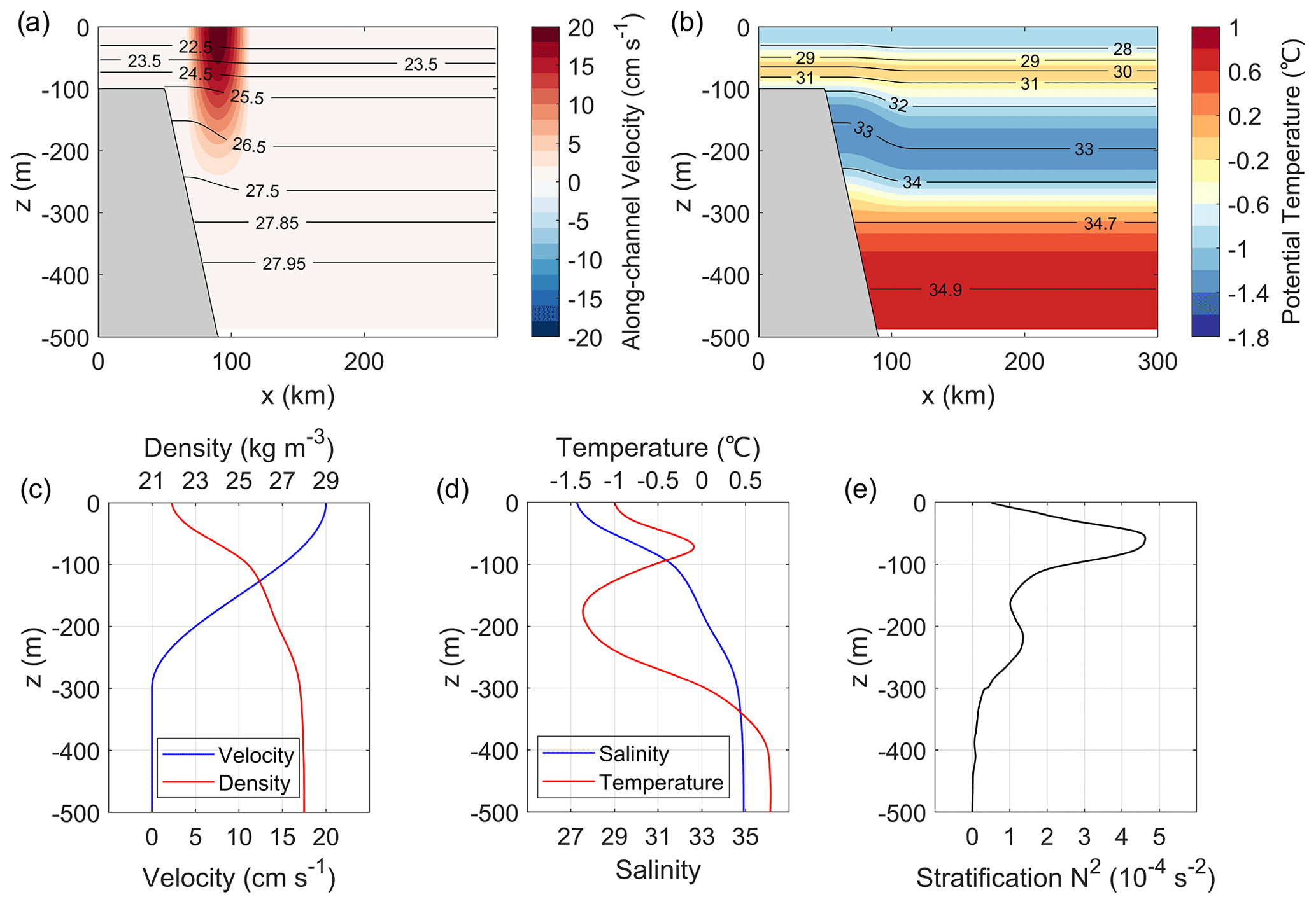
Figure 3 Initial conditions for the numerical experiments: (a) along-channel velocity (color) and isopycnals (black contours), (b) potential temperature (color) and isohalines (black contours), (c) vertical profiles of the along-channel velocity (blue) and density (red) at the flow center (x=90 km), (d) vertical profiles of the salinity (blue) and temperature (red) at x=90 km, and (e) vertical profile of the background mean stratification N².

The ice–ocean stress in the model is calculated from the ice velocity u_i and sea surface velocity u_s, following a quadratic drag law (Zhang and Hibler, 1997; Losch et al., 2010),

$$\begin{array}{}\text{(2)}& \mathit{\tau }=\mathit{\alpha }{\mathit{\rho }}_{\mathrm{0}}{C}_{Di}\left|{\mathit{u}}_{\mathrm{i}}-{\mathit{u}}_{\mathrm{s}}\right|\left({\mathit{u}}_{\mathrm{i}}-{\mathit{u}}_{\mathrm{s}}\right),\end{array}$$

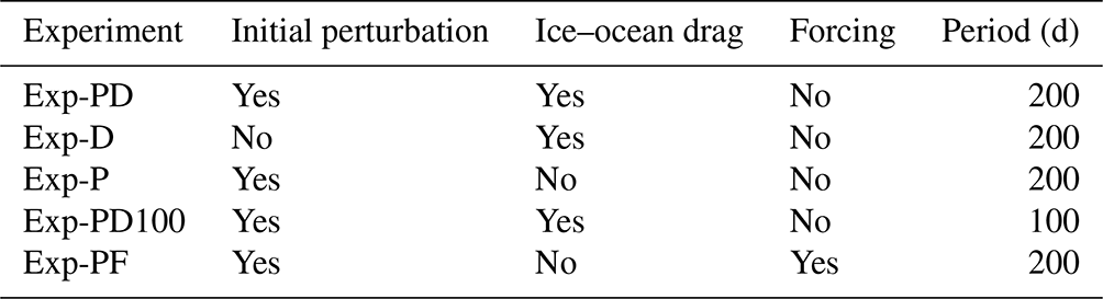
where α is ice concentration and $C_{Di}=\mathrm{5.5}\times {\mathrm{10}}^{-\mathrm{3}}$ is the drag coefficient. In the base experiment (Exp-PD; P and D stand for initial perturbation and ice–ocean drag, respectively), the ice–ocean drag is turned on and a random perturbation ($\stackrel{\mathrm{̃}}{u}$, $\stackrel{\mathrm{̃}}{v}$) is added to the initial velocity field to produce instabilities. The perturbation is weighted by 0.05vⁱⁿⁱ and given as

$$\begin{array}{}\text{(3)}& \left\{\begin{array}{l}\stackrel{\mathrm{̃}}{u}=\mathrm{0.05}{v}^{\mathrm{ini}}{A}_{\mathrm{1}},\\ \stackrel{\mathrm{̃}}{v}=\mathrm{0.05}{v}^{\mathrm{ini}}{A}_{\mathrm{2}},\end{array}\right.\end{array}$$

where A₁ and A₂ are three-dimensional random scalar fields between 0 and 1 drawn from the standard normal distribution (white noise). The resulting perturbation is of the order of 1 cm s⁻¹. The base experiment is a pure spin-down experiment and is integrated for 200 d. Four sensitivity experiments are also carried out to diagnose the effects of ice friction (see the details in Sect. 3.2).

2.2 Energetics calculations

We calculate the KE and available potential energy (APE) per unit volume (in units of J m⁻³) by

$$\begin{array}{}\text{(4)}& E_k={\displaystyle \frac{\mathrm{1}}{\mathrm{2}}}{\mathit{\rho }}_{\mathrm{0}}\left(u^{\mathrm{2}}+v^{\mathrm{2}}\right),\end{array}$$

and

$$\begin{array}{}\text{(5)}& E_p={\displaystyle \frac{g^{\mathrm{2}}{\left(\mathit{\rho }-{\mathit{\rho }}_r\right)}^{\mathrm{2}}}{\mathrm{2}{\mathit{\rho }}_{\mathrm{0}}{N}^{\mathrm{2}}}},\end{array}$$

with ρ being the output varying density and u and v the cross- and along-channel velocity components. Note that the vertical velocity w (order 10⁻⁵ m s⁻¹) is much smaller than u and v (order 0.1 m s⁻¹) and thus has little contribution to KE. It is not appropriate to separate the velocity field into its time-mean ($\stackrel{\mathrm{‾}}{u}$, $\stackrel{\mathrm{‾}}{v}$) and time-varying (u^′, v^′) parts and define the eddy kinetic energy (EKE) by ${\mathit{\rho }}_{\mathrm{0}}(u{{}^{\prime }}^{\mathrm{2}}+v{{}^{\prime }}^{\mathrm{2}})/\mathrm{2}$. This is because the slope current would change with time as a response to the ice friction such that v^′ is nonzero even when not encountering eddies. Namely, the EKE may be overestimated by ${\mathit{\rho }}_{\mathrm{0}}(u{{}^{\prime }}^{\mathrm{2}}+v{{}^{\prime }}^{\mathrm{2}})/\mathrm{2}$. Here we define the KE of the along-slope mean flow by

$$\begin{array}{}\text{(6)}& \widehat{E_k}={\displaystyle \frac{\mathrm{1}}{\mathrm{2}}}{\mathit{\rho }}_{\mathrm{0}}{\widehat{v}}^{\mathrm{2}},\end{array}$$

where $\widehat{v}$ is the along-channel average of v. The cross-channel velocity component u is classified into perturbation velocity and is not included in the calculation of the mean flow KE. Then, we use the difference $E_k-\widehat{E_k}$ to measure the EKE.

The rate at which the surface stress works on the ocean, i.e., the power input to the ocean from surface stress (in units of W m⁻²), can be written as a product of surface stress and surface current velocity (e.g., Wunsch, 1998; Zhai et al., 2012; Zhong et al., 2019). For the whole model domain, the power of ice friction (in units of W) is calculated by

$$\begin{array}{}\text{(7)}& P_{\mathit{\tau }}={\int }_{\mathrm{0}}^X{\int }_{\mathrm{0}}^Y\left(\mathit{\tau }\cdot {\mathit{u}}_{\mathrm{s}}\right)\mathrm{d}x\mathrm{d}y,\end{array}$$

where X=300 and Y=200 km. The time integral of P_τ gives the work done by the ice friction,

$$\begin{array}{}\text{(8)}& W_{\mathit{\tau }}\left(t\right)={\int }_{\mathrm{0}}^t{P}_{\mathit{\tau }}\mathrm{d}t.\end{array}$$

2.3 Linear instability calculations

We analyze the baroclinic instability of the slope current based on the linearized quasi-geostrophic PV equation (Smith, 2007; Tulloch et al., 2011; Meneghello et al., 2021):

$$\begin{array}{}\text{(9a)}& {\displaystyle }\left({\displaystyle \frac{\partial }{\partial t}}+\mathit{U}\cdot {\mathrm{\nabla }}_{\mathrm{h}}\right)q+\mathit{u}\cdot {\mathrm{\nabla }}_{\mathrm{h}}Q=\mathrm{0},\text{(9b)}& {\displaystyle }q={\mathrm{\nabla }}_{\mathrm{h}}^{\mathrm{2}}\mathit{\psi }+{\displaystyle \frac{\partial }{\partial z}}\left({\displaystyle \frac{f^{\mathrm{2}}}{N^{\mathrm{2}}}}{\displaystyle \frac{\partial \mathit{\psi }}{\partial z}}\right),\text{(9c)}& {\displaystyle }{\mathrm{\nabla }}_{\mathrm{h}}Q=-{\displaystyle \frac{\partial }{\partial z}}\left({\displaystyle \frac{f^{\mathrm{2}}}{N^{\mathrm{2}}}}\mathit{k}\times {\displaystyle \frac{\partial \mathit{U}}{\partial z}}\right),\end{array}$$

where q is the perturbation PV, ψ is the perturbation streamfunction, and $\mathit{u}=\mathit{k}\times {\mathrm{\nabla }}_{\mathrm{h}}\mathit{\psi }$ is the perturbation horizontal velocity (k is the upward unit vector and ∇_h is the horizontal gradient operator). The relative vorticity of the mean flow is neglected as it is small compared to f. The ratio of the background mean relative vorticity to f can be scaled as $V/fL$ (V and L are velocity and horizontal length scales of the mean flow), which is only 0.1 for V=0.1 m s⁻¹ and L=10 km. The background PV gradient ∇_hQ on the f plane is simplified as a function of the background horizontal velocity U and stratification N², which varies only with depth. Surface (z=0) and bottom ($z=-h$) boundary conditions for Eq. (9) are provided by Williams and Robinsonm (1974), Pedlosky (1987), and Meneghello et al. (2021):

$$\begin{array}{}\text{(10a)}& {\displaystyle }\begin{array}{rl}\left({\displaystyle \frac{\partial }{\partial t}}+U\cdot {\mathrm{\nabla }}_{\mathrm{h}}\right){\displaystyle \frac{\partial \mathit{\psi }}{\partial z}}& ={\displaystyle \frac{\partial U}{\partial z}}\cdot {\mathrm{\nabla }}_{\mathrm{h}}\mathit{\psi }\\ & -{\displaystyle \frac{N^{\mathrm{2}}}{f}}{\displaystyle \frac{d_{\mathrm{s}}}{\mathrm{2}}}{\mathrm{\nabla }}_{\mathrm{h}}^{\mathrm{2}}\mathit{\psi },z=\mathrm{0},\end{array}\text{(10b)}& {\displaystyle }\begin{array}{rl}\left({\displaystyle \frac{\partial }{\partial t}}+U\cdot {\mathrm{\nabla }}_{\mathrm{h}}\right){\displaystyle \frac{\partial \mathit{\psi }}{\partial z}}& ={\displaystyle \frac{\partial U}{\partial z}}\cdot {\mathrm{\nabla }}_{\mathrm{h}}\mathit{\psi }\\ & +{\displaystyle \frac{N^{\mathrm{2}}}{f}}{\displaystyle \frac{d_{\mathrm{b}}}{\mathrm{2}}}{\mathrm{\nabla }}_{\mathrm{h}}^{\mathrm{2}}\mathit{\psi },z=-h,\end{array}\end{array}$$

where d_s and d_b are the surface and bottom Ekman layer depths, and $d_{\mathrm{s}}{\mathrm{\nabla }}_{\mathrm{h}}^{\mathrm{2}}\mathit{\psi }/\mathrm{2}$ and $d_{\mathrm{b}}{\mathrm{\nabla }}_{\mathrm{h}}^{\mathrm{2}}\mathit{\psi }/\mathrm{2}$ are the corresponding Ekman pumping. Typically, the surface Ekman layer depth of the order of 10 m is equivalent to the vertical diffusivity ${\mathit{\upsilon }}_{\mathrm{E}}=d_{\mathrm{s}}^{\mathrm{2}}f/\mathrm{2}$ of approximately 10⁻² m⁻² s⁻¹.

Because the background PV gradient is in the west–east direction, the waves traveling in the north–south direction can most easily draw energy from the background mean flow. For simplicity, we ignore west–east wave propagation and assume a plane-wave solution of the form $\mathit{\psi }=\widehat{\mathit{\psi }}\left(z\right)e^{i\left(ly-\mathit{\omega }t\right)}$, where $\widehat{\mathit{\psi }}$ is the vertical structure of the perturbation, l is the along-channel wavenumber, and $\mathit{\omega }={\mathit{\omega }}_r+i{\mathit{\omega }}_{\mathrm{i}}$ is the complex frequency. If the imaginary frequency component ω_i is positive, the corresponding mode is unstable and will grow exponentially with time on a timescale of $\mathrm{1}/{\mathit{\omega }}_{\mathrm{i}}$. Substitution of the plane-wave solution into Eq. (9) yields a generalized eigenvalue problem, with ω being the eigenvalues and $\widehat{\mathit{\psi }}$ the eigenvectors. The eigenvalue problem is then discretized on the staggered vertical model grid and solved numerically following the algorithm proposed by Smith (2007). Bottom topography is not considered as we calculate the background PV gradient from the velocity and density profiles at the center of the front, offshore of the continental slope.

3 Results

3.1 Base experiment

3.1.1 Generation of subsurface eddies

In the initial state the slope current is surface-intensified, so the normalized relative vorticity $\mathit{\zeta }/f$ is larger at the surface than the subsurface ($z=-\mathrm{105}$ m) (Fig. 4a and b). Due to the presence of ice friction in Exp-PD, the surface vorticity decays quickly with time while the subsurface vorticity remains large (Fig. 4c–h). On day 60 the perturbations are visible in the subsurface (Fig. 4d), which then grow into eddies as shown in Fig. 4f and h. The growth of subsurface eddies corresponds to an increase in the subsurface KE (Fig. 5c). The total KE also increases after day 60 (Fig. 5a, black curve), while the mean flow KE remains small and starts to decrease on day 100 (Fig. 5a, red curve). This gives rise to a continuous increase in EKE since day 60 (the distance between the two curves keeps increasing). The curve of the natural log of EKE shows that the perturbations have started to grow around day 30 (Fig. 5b), but the EKE is not large enough to be seen until day 60. The slope of that curve represents the exponential growth rate of EKE, which is ∼ 0.1 d⁻¹ for the growth period from day 30 to 90.

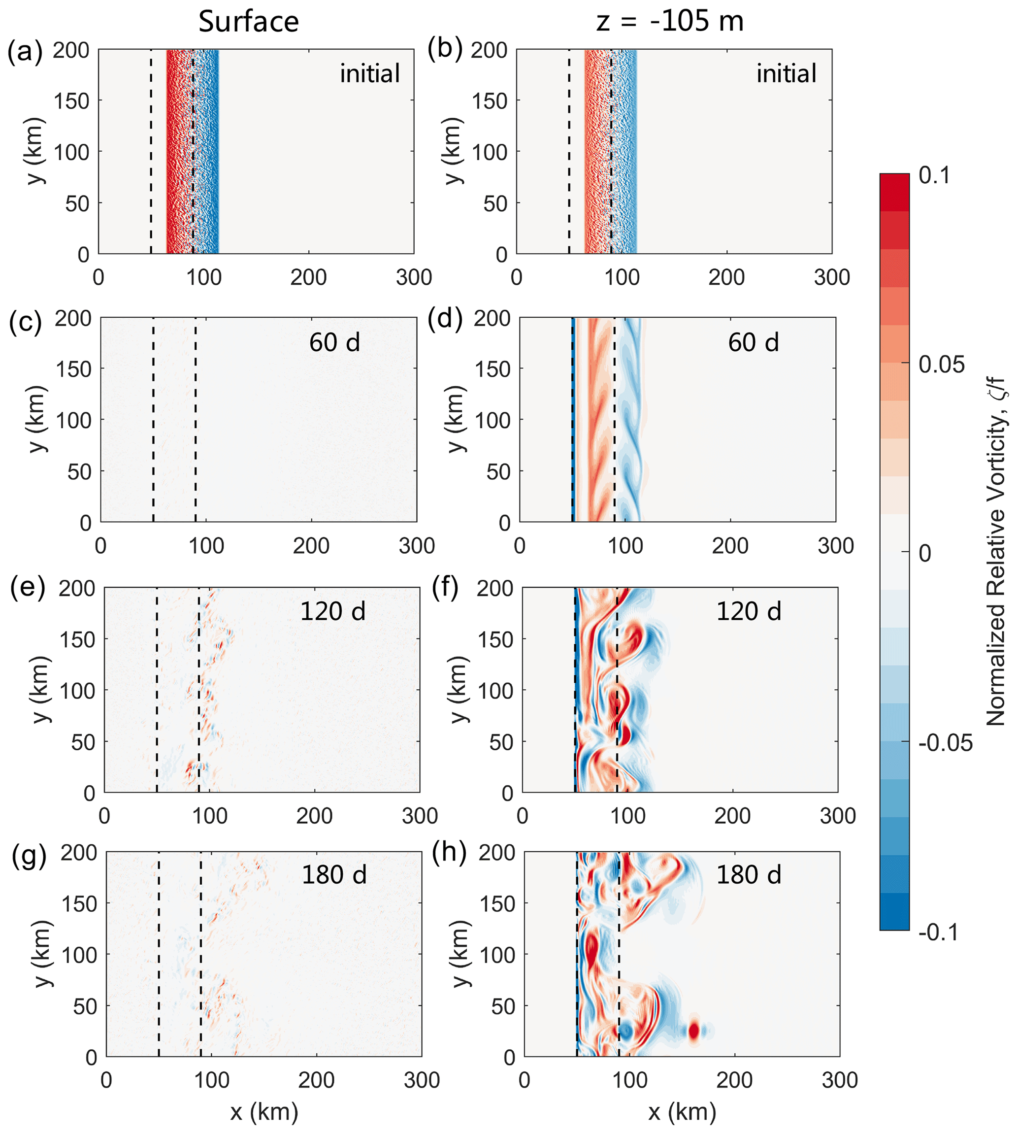
Figure 4 Distributions of the relative vorticity $\mathit{\zeta }=\partial v/\partial x-\partial u/\partial y$ normalized by f at $t=\mathrm{0},\mathrm{60}$, 120, and 180 d from Exp-PD: (left) at the surface and (right) at the depth of −105 m. The region of the continental slope is outlined by two dashed black lines in each panel.

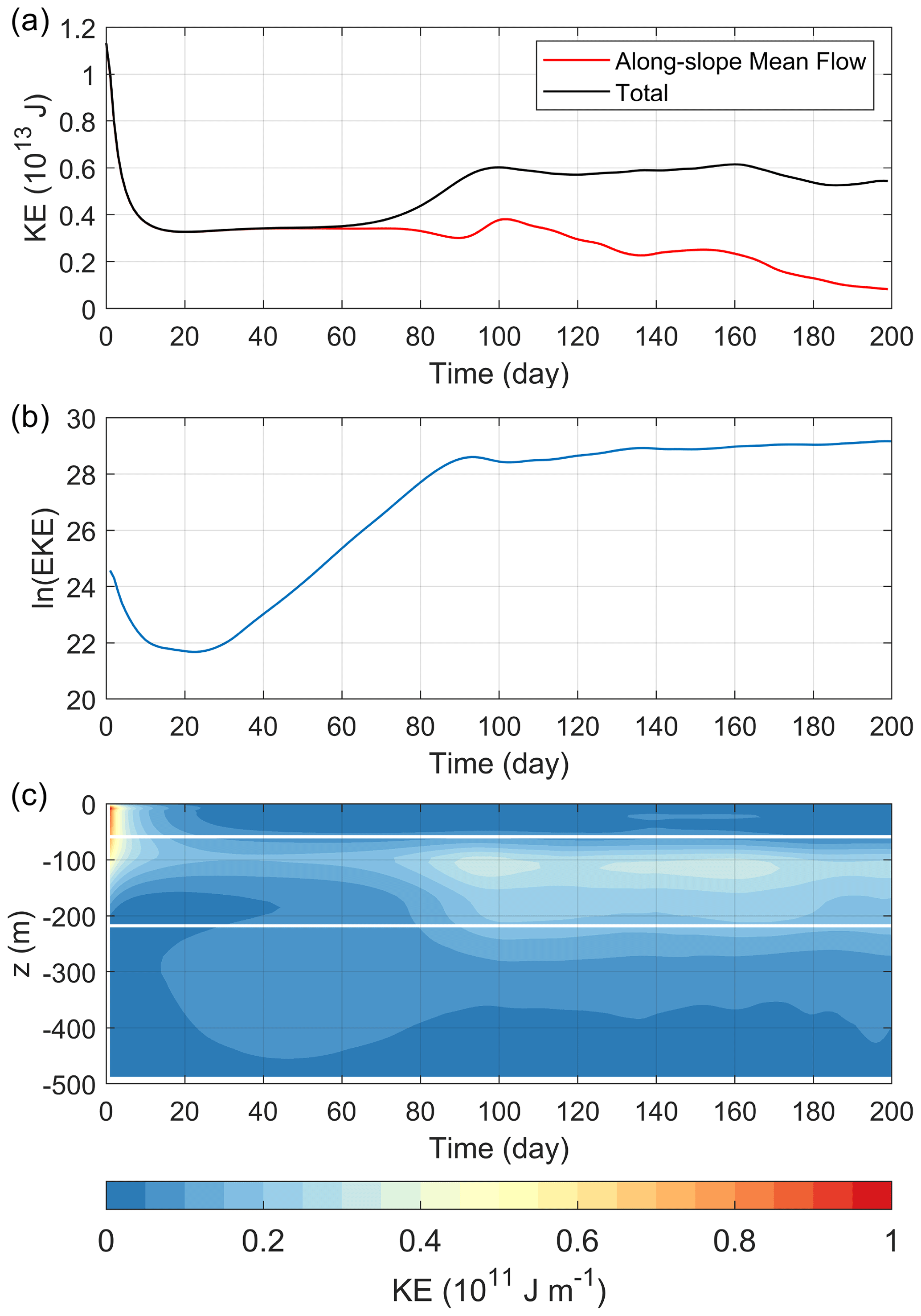
Figure 5 (a) Time evolution of the KE of the along-slope mean flow (red curve) and the total KE integrated over the model domain (black curve) from Exp-PD. (b) Time evolution of the natural log of the EKE integrated over the model domain from Exp-PD. (c) Time–depth plot of the horizontal integral of KE from Exp-PD. The white lines mark the depths of the two stratification peaks (−59 and −218 m).

The mechanism for the generation of subsurface eddies in the interior Arctic Ocean has been investigated by Meneghello et al. (2021) through linear baroclinic instability analysis. Specifically, they found that the strong stratification at the depth of around −50 m can protect the underlying unstable modes from the effect of ice friction so that subsurface eddies can develop. With the output density and velocity profiles at x=90 km on day 60, we calculate the growth rate ω_i and amplitude $\left|\widehat{\mathit{\psi }}\right|$ for the wavenumber range ${\mathrm{10}}^{-\mathrm{6}}<l<\mathrm{1}$ m⁻¹. The results show three unstable branches, including a halocline branch and two surface branches (Fig. 6).

The surface unstable modes have length scales (defined as $\mathrm{1}/l)$ ranging from a few meters to 10 km so that only the longest surface waves can be fully resolved by the numerical model. Note that a few small-scale signals are visible in the surface vorticity field (e.g., Fig. 4e and g). Since the instability calculations are based on the quasi-geostrophic assumption, the results for length scales down to O(1 m) are not valid. The fastest-growing mode for the halocline branch has a length scale of 10 km, which is the same as our estimated baroclinic deformation radius. The vertical profile of EKE in Exp-PD approximately follows the square of the amplitude of the fastest-growing halocline mode, and both of them reach the maximum at a depth of around −100 m (Fig. 6b). Therefore, the generation of subsurface eddies should be due to the growth of the halocline mode. It is noted that the halocline mode grows at a rate of ∼ 0.2 d⁻¹, which is faster than the growth of the EKE in Exp-PD (∼ 0.1 d⁻¹ for the period from day 30 to 90). This is because the background velocity and density profiles used in the linear instability calculations are taken from the center of the front, where the PV gradient is the strongest. In other regions the PV gradient is weaker and the corresponding growth rate is smaller. It takes time for the eddies to spread over the model domain. The linear instability calculations may also overestimate the growth rate since the interior viscosity is not considered.

The ice friction is known to suppress the growth of surface unstable modes (Meneghello et al., 2021). As we change the surface Ekman layer depth from 0 to 20 m, the maximum growth rate of the surface modes decreases from ∼ 2.2 to 0.4 d⁻¹ (Fig. 6a, blue lines). However, the growth of the halocline mode is not sensitive to the ice friction (Fig. 6a, black lines), and varying the surface Ekman layer depth only causes a slight change in the vertical structure (Fig. 6b, black lines).

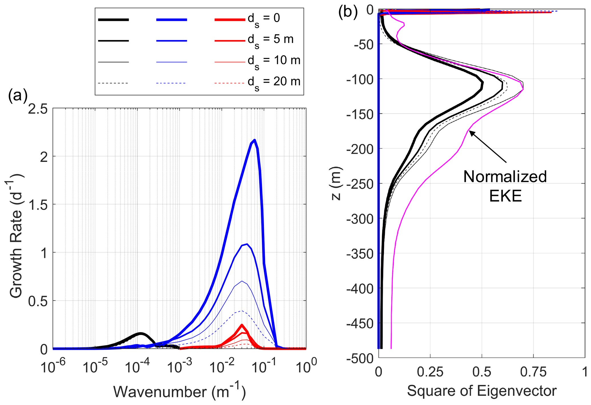
Figure 6 (a) Growth rate ω_i of unstable modes as a function of wavenumber for the surface Ekman layer depth d_s = 0, 5, 10, and 20 m, as well as the bottom Ekman layer depth d_b=20 m. Three unstable branches are resolved, including a halocline branch (black) and two surface branches (blue and red). (b) Square of the eigenvector ${\widehat{\mathit{\psi }}}^{\mathrm{2}}$ of the most unstable mode for each unstable branch. The magenta curve in (b) is the vertical profile of EKE (from Exp-PD, averaged over the final 100 d) normalized by the maximum ${\widehat{\mathit{\psi }}}^{\mathrm{2}}$ of the halocline mode.

3.1.2 Evolution of the flow structure

Figure 7a shows a symmetric distribution of downwelling and upwelling at t = 5 d, which is driven by the spatially variable friction between the ice and surface mean flow (Leng et al., 2022). The streamfunction obtained by integrating the vertical velocity along x presents an anticlockwise overturning circulation (Fig. 7b). Such overturning can modify the vertical structure of the mean flow. On the one hand, the downwelling and upwelling components in the overturning can cause vertical density fluxes and force the near-surface isopycnals to be tilted in the opposite direction to the deeper ones. On the other hand, the upper arm of overturning fed by the Ekman transport is convergent (divergent) on the west (east) side of the mean flow, which reduces the gradient of sea surface height and thus weakens the surface geostrophic velocity. As a result, a subsurface velocity core is formed at a depth of approximately −100 m where the isopycnal slope is zero (via geostrophic setup) (Fig. 7c). Furthermore, the overturning can reach the bottom and drive a countercurrent extending from the shelf break to the open ocean. The onshore part of the countercurrent is trapped by the sloping bottom, with the maximum velocity occurring in the vicinity of the shelf break. Offshore of the continental slope, the countercurrent is weaker and spans wider ranges of distance and depth.

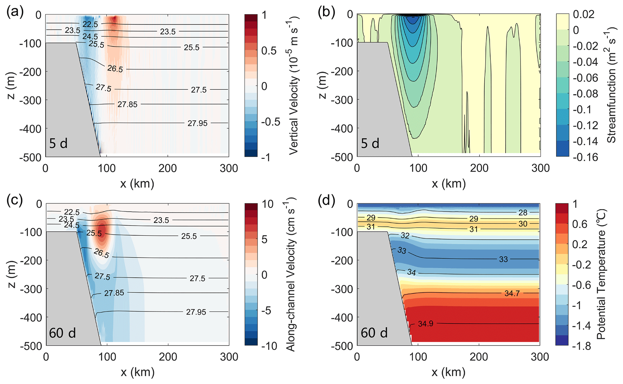
Figure 7 (a) Vertical velocity (color) overlain by isopycnals (black contours) and (b) overturning streamfunction averaged between y=0 and 200 km at t = 5 d. (c) Along-channel velocity (color) overlain by isopycnals (black contours) and (d) potential temperature (color) overlain by isohalines (black contours) averaged between y = 0 and 200 km at t = 60 d.

One may think that the ice-induced overturning would produce diapycnal transport since the overturning streamlines intersect the isopycnals at t=5 d (Fig. 7a and b). However, this is not a steady state since the overturning and isopycnals are evolving. The overturning diminishes quickly along with the decay of Ekman pumping, and meanwhile, the isopycnals get displaced instead of staying at the same depth. On day 60 the potential temperature remains distributed following isohalines (or isopycnals) (Fig. 7d). This indicates that the overturning does not drive significant diapycnal transport.

3.2 Comparison between the base and sensitivity experiments

In addition to the base experiment, we carry out four sensitivity experiments to further investigate the role of ice friction in the energetics of the slope current (Table 1). Three of them are pure spin-down experiments (Exp-D, Exp-P, and Exp-PD100) since no wind forcing is applied. In Exp-D, we keep the ice–ocean drag and remove the initial perturbation to focus on the evolution induced by the ice friction (note that this is nearly a two-dimensional calculation). In Exp-P, we turn off the ice–ocean drag and include the initial perturbation. This allows instabilities to grow without the influence of surface forces. Exp-PD100 is a restart of Exp-P from day 100 and is run for 100 d with the ice–ocean drag (the initial conditions for Exp-PD100 are taken from the output of Exp-P on day 100). This restart experiment aims to examine the effect of ice friction on pre-existing eddies. The results for the first 100 d of Exp-PD100 presented below are actually from Exp-P. The last experiment, Exp-PF, has no sea ice model and is forced by the surface stress, shortwave radiation, and heat and freshwater fluxes at the surface of the ocean diagnosed from the daily output of Exp-PD. This will help distinguish the relative influence of baroclinic instability versus Ekman pumping on the release of APE. Each simulation is integrated for 200 d except for Exp-PD100.

Table 1 The setup for the base and sensitivity experiments.

3.2.1 Evolution of KE and APE

As mentioned above in Sect. 3.1, the time evolution of KE in Exp-PD should be related to the ice friction as well as the generation of subsurface eddies through baroclinic instability. This can be further illustrated by the results from the sensitivity experiments. In Exp-D, a rapid loss of KE occurs in the first 10 d as in Exp-PD (Fig. 8a, solid and dashed black curves). The APE in Exp-D also decreases from the beginning (Fig. 8b, dashed black curve) but the baroclinic conversion is not allowed because the initial perturbation is removed (the flow is two-dimensional). Since no eddies are generated in Exp-D, the KE remains low until the end of the simulation.

The ice–ocean drag is turned off in Exp-P, and hence there is almost no change in KE in the first 60 d (Fig. 8a, blue solid curve). The increase in KE from day 60 to 100 is $\sim \mathrm{1}\times {\mathrm{10}}^{\mathrm{13}}$ J in Exp-P, which is 3 times that in Exp-PD. Figure 9b shows two KE maxima in the vertical in Exp-P after day 80. The deeper KE maximum at a depth of around −100 m is due to the growth of the halocline mode, while the upper KE maximum at the surface arises from both the surface and halocline modes. Note that the surface vorticity field in Exp-P is dominated by small-scale perturbations, but it also presents mesoscale features similar to those in the subsurface (compare Fig. 10c and d). This is due to the fact that the halocline mode extends to the surface, although the eigenvector amplitude at the surface is very small (Fig. 6b). The APE in Exp-P appears to be steady in the first 60 d, and then it undergoes a rapid reduction ($\sim \mathrm{1.5}\times {\mathrm{10}}^{\mathrm{13}}$ J) between day 60 and 100 (Fig. 8b, blue solid curve), as the KE increases by $\sim \mathrm{1}\times {\mathrm{10}}^{\mathrm{13}}$ J due to the growth of eddies (Fig. 8a, blue solid curve). Namely, the eddies draw energy from the APE stored in the slope current via baroclinic conversion. Note that the KE is also being dissipated by the interior viscosity and bottom friction. Although the APE continues to decrease to the end of Exp-P, the KE field plateaus from day 100. This suggests that the loss of KE due to dissipation is of the same magnitude as the energy conversion from APE to KE after day 100.

In the restart experiment (Exp-PD100), the KE drops quickly from day 100 as a response to the ice friction (Fig. 8a, dashed blue curve). The reduction of KE in Exp-PD100 occurs at all depths and is more significant in the upper 60 m (Fig. 9c). The subsurface KE maximum shielded by the shallower stratification peak remains at ∼ 100 m depth to the end of the calculation. The APE in Exp-PD100 decreases more quickly than in Exp-P after day 100 (Fig. 8b), which is related to the ice-induced Ekman pumping (this is discussed below in Sect. 3.2.2).

Exp-PF includes the same Ekman pumping as Exp-PD but there is no damping of eddies by interaction with ice. Much of the APE in Exp-PF is reduced by the large-scale Ekman pumping instead of being converted into EKE through baroclinic instability, and thus Exp-PF has lower EKE than Exp-P (Fig. 8a). However, the large-scale Ekman pumping does not damp the perturbations directly, so EKE in Exp-PF is higher than in Exp-PD, mostly in the upper 50 m (see the vertical structure of KE in Fig. 9d and surface relative vorticity field in Fig. 10g). Because eddies also contribute to APE release, the APE in Exp-PF is slightly lower than in Exp-PD after eddies form (Fig. 8b).

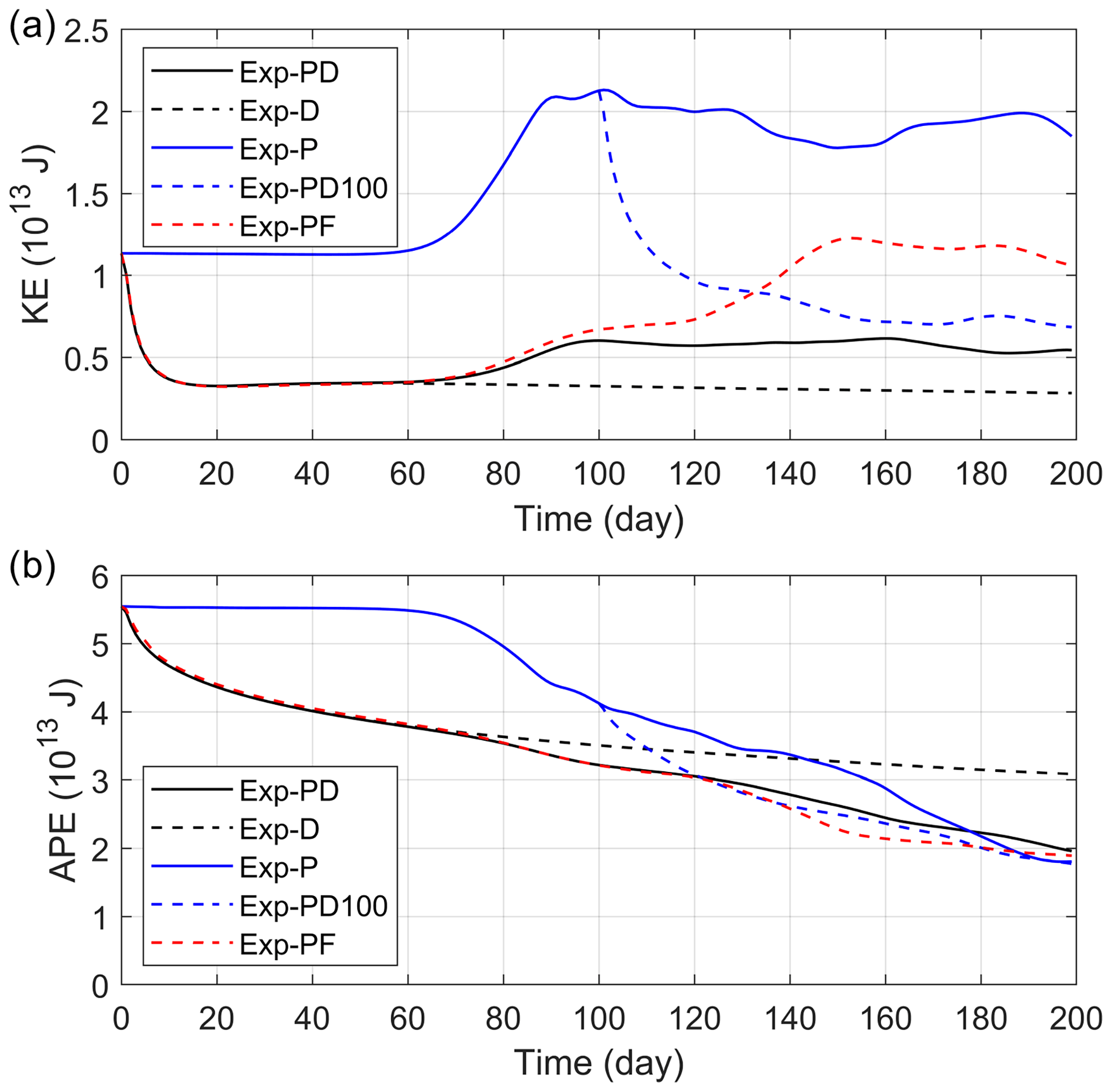
Figure 8 Time evolution of the (a) KE and (b) APE integrated over the model domain from the base and sensitivity experiments.

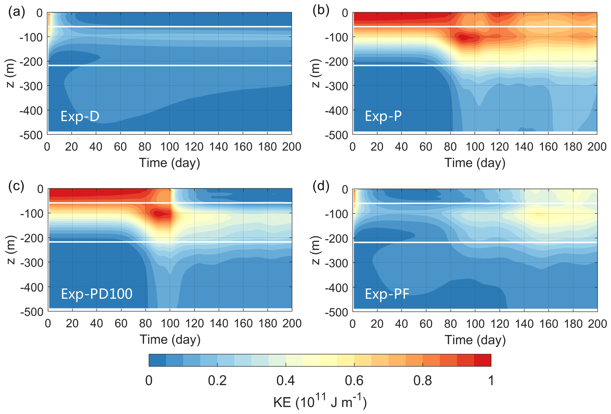
Figure 9 Time–depth plot of the horizontal integral of KE from the four sensitivity experiments. The white lines in each panel mark the depths of the two stratification peaks (−59 and −218 m).

Figure 10 Distributions of the normalized relative vorticity $\mathit{\zeta }/f$ from the four sensitivity experiments at t = 180 days: (left) at the surface and (right) at the depth of −105 m. The region of the continental slope is outlined by two dashed black lines in each panel.

3.2.2 Work done by the ice friction

The ice cover acts as a nearly immobile surface lid in our experiments ($\left|{\mathit{u}}_{\mathrm{i}}\right|<{\mathrm{10}}^{-\mathrm{4}}$ m s⁻¹) because the ice concentration is high and the ice internal stress is strong enough to counteract the ice–ocean stress and prevent the ice from drifting together with the current. Therefore, the ice–ocean stress is nearly in the opposite direction to the sea surface velocity ($\mathit{\tau }\cdot {\mathit{u}}_{\mathrm{s}}<\mathrm{0}$) and does negative work on the ocean. In both Exp-PD and Exp-D the work done by the ice friction has reached $-\mathrm{2}\times {\mathrm{10}}^{\mathrm{13}}$ J by the end of the simulation (Fig. 11a and b, red curves), contributing to more than half of the loss in total mechanical energy (sum of APE and KE) (Fig. 11a and b, black curves). The rest of the energy loss should be due to the interior viscosity and bottom friction (measured by the difference between the black and red curves), which increases with time and appears to be more significant in the cases in which eddies are well developed (Fig. 11c and d). Since the ice–ocean drag is turned off in Exp-P, there is no mechanical energy lost through the ice–ocean interface (Fig. 11c). In this case, the mechanical energy can be dissipated only by interior viscosity and bottom friction. In Exp-PD100 the ice friction only works for 100 d, while it finally results in a reduction of $-\mathrm{2}\times {\mathrm{10}}^{\mathrm{13}}$ J in mechanical energy, comparable to the dissipation due to interior viscosity and bottom friction (Fig. 11d). Figure 11e shows that, from day 100 onwards, the surface stress puts a small amount of energy back into the ocean. This is because the surface stress diagnosed from Exp-PD does not always damp the surface eddies in Exp-PF. When $\mathit{\tau }\cdot {\mathit{u}}_{\mathrm{s}}>\mathrm{0}$, the surface stress can do positive work on the eddies.

Figure 11 The change in mechanical energy (sum of APE and KE) relative to t = 0 (black solid curve) and the work done by the surface stress (red solid curve) integrated over the model domain as functions of time from the base and sensitivity experiments. The dashed black curve in each panel indicates the change in APE.

As mentioned above in Sect. 3.1.2, the ice friction drives Ekman pumping to modulate the isopycnal slopes, and this is likely to cause the release of APE. To better illustrate the role of ice-induced Ekman pumping, we introduce a simplified density equation:

$$\begin{array}{}\text{(11)}& {\displaystyle \frac{\partial \mathit{\rho }}{\partial t}}+w{\displaystyle \frac{\partial {\mathit{\rho }}_r}{\partial z}}=\mathrm{0},\end{array}$$

which assumes that the local density would change as the vertical velocity advects a background mean density gradient (the horizontal advection terms are neglected). This is more restrictive than the quasi-geostrophic approximation and is valid for Exp-D, wherein the geostrophic flow is nearly two-dimensional (u_g≈0) and the change in density in the along-channel direction is small ($\partial \mathit{\rho }/\partial y\approx \mathrm{0}$); i.e., the horizontal advection by the geostrophic flow is negligible. Combining Eqs. (5) and (11), we obtain a rate at which the APE changes (in units W m⁻³):

$$\begin{array}{}\text{(12)}& {\displaystyle \frac{\partial E_p}{\partial t}}=g\left(\mathit{\rho }-{\mathit{\rho }}_r\right)w,\end{array}$$

where (ρ−ρ_r)w is the vertical density flux. This equation suggests that the APE would be released if the lighter water (relative to the area-mean density) were advected upward or the denser water moved downward. This is the case in Exp-D wherein the ice-induced Ekman pumping (see, e.g., Fig. 7a) results in a negative density flux that dominates the release of APE (Fig. 12b, the two curves are nearly identical). Furthermore, the integrated g(ρ−ρ_r)w agrees well with $\partial E_p/\partial t$ in Exp-PD, Exp-P, and Exp-PD100 (Fig. 12a, c, and d), suggesting that Eqs. (11) and (12) are valid even when eddies are generated. The most significant bias between g(ρ−ρ_r)w and $\partial E_p/\partial t$ occurs in Exp-PF (Fig. 12e), wherein both the surface stress and eddies contribute to the horizontal advection of density. In this case the horizontal advection terms are important and should not be ignored.

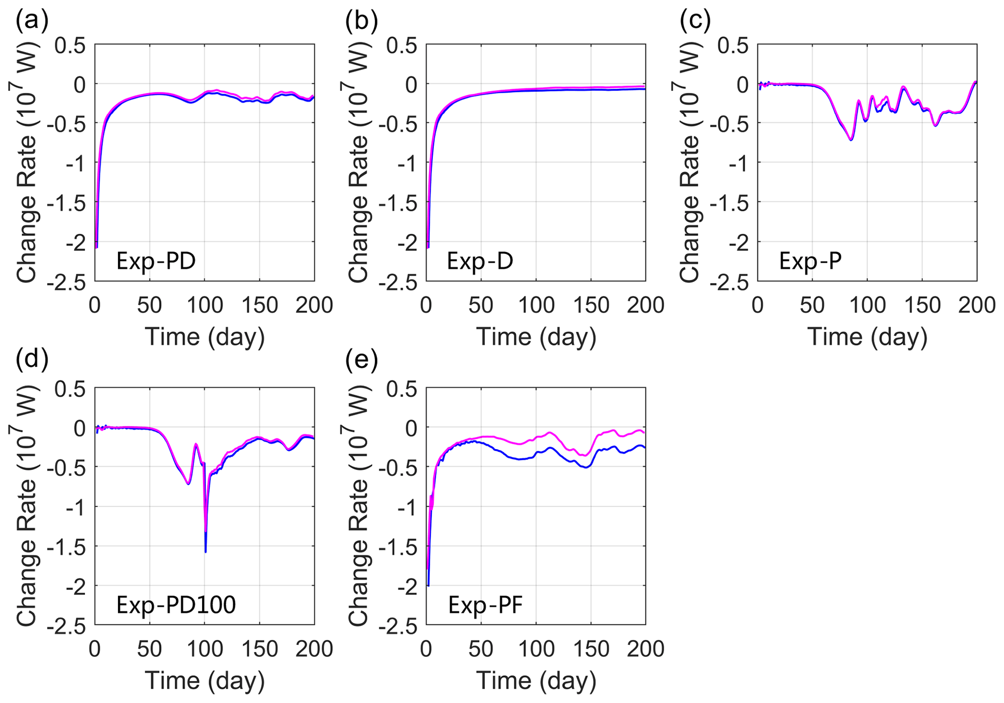
Figure 12 The change rate of APE (magenta curve) and g(ρ−ρ_r)w (blue curve) integrated over the model domain as functions of time from the base and sensitivity experiments.

Figure 12 shows that both the ice friction and eddies can produce negative density flux to release APE. The eddy-induced density flux means energy transfer from APE to EKE through baroclinic instability and the ice friction does negative work on the ocean via modifying the density and velocity structures (the isopycnal slope is reduced when the density flux is negative). In Exp-D, as the APE is released by the ice-induced density flux and the KE decreases due to Ekman pumping (Fig. 8, dashed black lines), the total mechanical energy gets lost (Fig. 11b). The relative importance of the Ekman pumping versus baroclinic instability for the release of APE is indicated by the difference between Exp-P (no Ekman pumping) and Exp-PF (with Ekman pumping). The EKE is significantly less in Exp-PF (Fig. 9d), both near the surface and at −100 m, because more APE is released by Ekman pumping rather than being converted to EKE through baroclinic instability.

For existing eddies, the friction between the ice and eddies is spatially variable and thus gives rise to strong Ekman pumping (see the case in Fig. 13). As the ice-induced Ekman pumping penetrates into deep water, it enhances the vertical velocity and produces stronger density flux (Fig. 14b and d) compared to that induced only by eddies (Fig. 14a and c). To better illustrate the impact of Ekman pumping over eddies, we define the perturbation density ρ^′ and vertical velocity w^′ as the deviations from the along-channel mean and use $\left({\mathit{\rho }}^{\prime }-{\mathit{\rho }}_r\right)w^{\prime }$ to represent the perturbation vertical density flux. The averaged $g\left({\mathit{\rho }}^{\prime }-{\mathit{\rho }}_r\right)w^{\prime }$ over the model domain is −9.4 W m⁻² in Exp-PD100 (with ice friction), which is more than twice the value in Exp-P (−4.1 W m⁻², without ice friction). This demonstrates that the ice-induced Ekman pumping over eddies can cause a net loss of APE. Note that this is essentially the same mechanism as for the mean flow and thus the sign of density flux is independent of the sense of vorticity of the eddy (cyclonic or anticyclonic), although the magnitude would change if we considered the relative vorticity in the Ekman transport calculation.

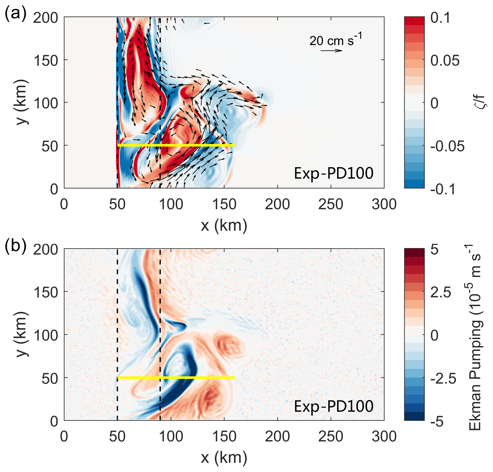
Figure 13 Distributions of (a) the surface-normalized relative vorticity $\mathit{\zeta }/f$ and velocity vectors faster than 5 cm s⁻¹ as well as (b) ice-induced Ekman pumping at t = 101 d from Exp-PD100. The yellow line marks a cross-channel section spanning x = 50 to 110 km at y = 50 km.

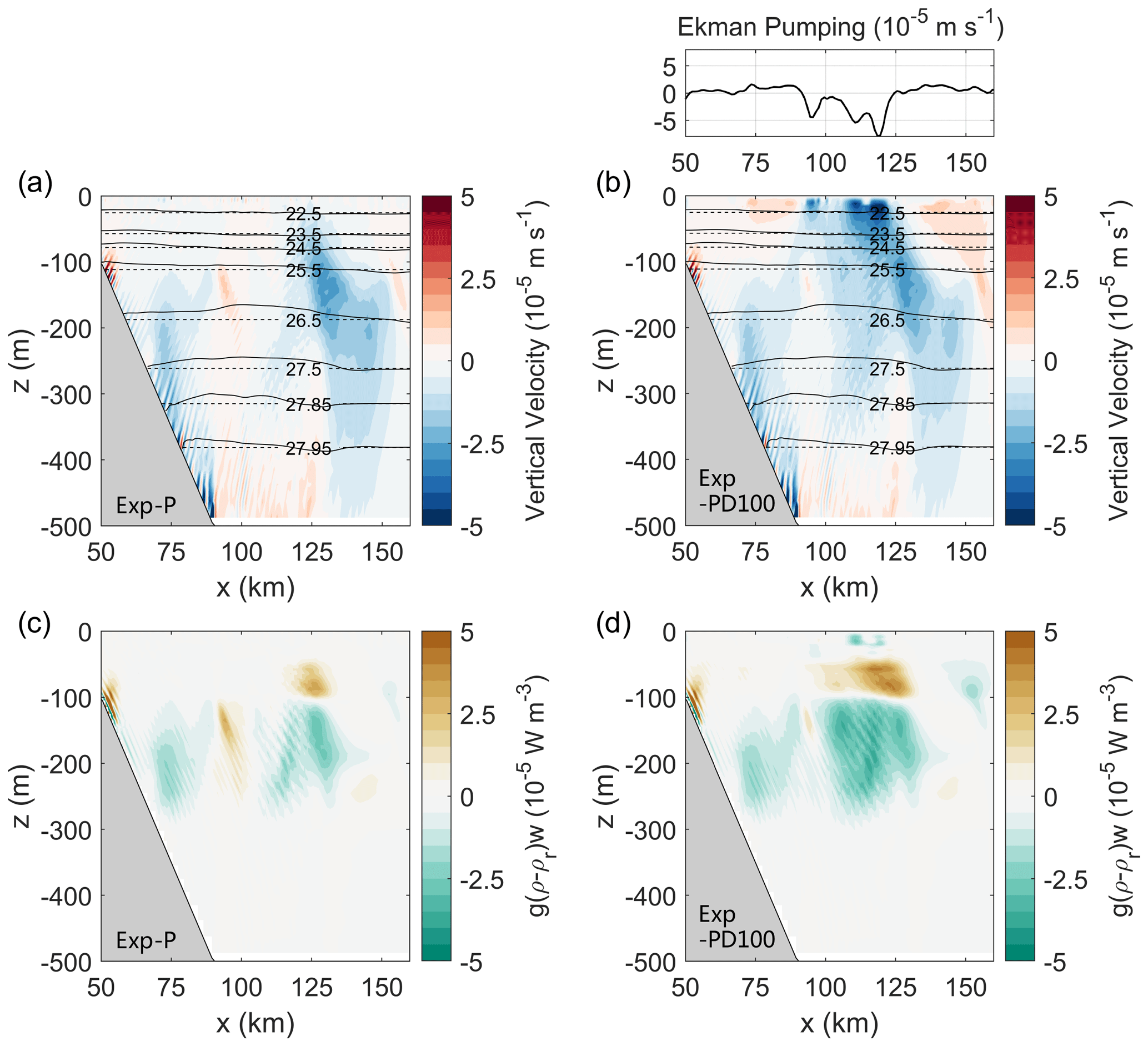
Figure 14 Vertical sections of (a, b) the vertical velocity (color) overlain by isopycnals (black solid contours) and (c, d) g(ρ−ρ_r)w at t = 101 d (see the location of the section in Fig. 13). The left column is from Exp-P and the right column is from Exp-PD100. The dashed black lines in (a) and (b) indicate the area-mean density profile. Above panel (b) is the Ekman pumping at t = 101 d from Exp-PD100.

3.3 Scaling estimates for the change in APE

The results presented above indicate that both the ice-induced Ekman pumping and baroclinic instability have contributions to the change in APE. Here we summarize some scales that may be useful to measure their relative importance.

The rate of conversion from mean APE to EKE (in units of W m⁻²) through baroclinic instability can be calculated following Gill et al. (1974) and Smith (2007):

$$\begin{array}{}\text{(13)}& R_{\mathrm{BC}}={\displaystyle \frac{{\mathit{\rho }}_{\mathrm{0}}{v}_{\max }^{\mathrm{2}}}{\mathrm{2}}}{\int }_{-h}^{\mathrm{0}}{\displaystyle \frac{f^{\mathrm{2}}}{N^{\mathrm{2}}}}{\displaystyle \frac{\mathrm{d}\mathit{\theta }}{\mathrm{d}z}}{\left({\displaystyle \frac{\left|\widehat{\mathit{\psi }}\right|}{{\left|\widehat{\mathit{\psi }}\right|}_{\max }}}\right)}^{\mathrm{2}}{\displaystyle \frac{\mathit{K}}{{\left|\mathit{K}\right|}^{\mathrm{2}}}}\cdot {\displaystyle \frac{\mathrm{d}\mathit{U}}{\mathrm{d}z}}\mathrm{d}z,\end{array}$$

where v_max is the maximum eddy velocity, $\mathit{\theta }={\tan }^{-\mathrm{1}}\left({\widehat{\mathit{\psi }}}_{\mathrm{i}}/{\widehat{\mathit{\psi }}}_r\right)$ is the phase of $\widehat{\mathit{\psi }}$ (note that the eigenvector can be written as $\widehat{\mathit{\psi }}=\left|\widehat{\mathit{\psi }}\right|e^{i\mathit{\theta }}={\widehat{\mathit{\psi }}}_r+i{\widehat{\mathit{\psi }}}_{\mathrm{i}}$), and K is the wavenumber vector. From Eq. (13), the baroclinic instability conversion rate may be scaled as $R_{\mathrm{BC}}=O\left({\mathit{\rho }}_{\mathrm{0}}{V}_{\mathrm{e}}^{\mathrm{2}}VIH/L^{\mathrm{2}}\right)$, where V_e is the order of eddy velocity and I is the horizontal scale of the fastest-growing mode.

The ice-induced Ekman pumping helps release the APE over a vertical scale $H=fL/N$. If we take $f={\mathrm{10}}^{-\mathrm{4}}$ s⁻¹, L=10 km, and $N={\mathrm{10}}^{-\mathrm{2}}$ s⁻¹, the vertical scale is estimated to be 100 m. This is much deeper than the Ekman layer, where the direct influence of surface stresses is confined (note that Ekman pumping could affect deeper depths for larger-scale flows). The rate at which the APE changes due to Ekman pumping can be estimated by g(ρ−ρ_r)w, where $\mathit{\rho }-{\mathit{\rho }}_r=O\left[{\mathit{\rho }}_{\mathrm{0}}fLV/\left(gH\right)\right]$ is derived from the thermal wind relation and $w=O\left[C_{Di}{V}^{\mathrm{2}}/\left(fL\right)\right]$ is of the same order as Ekman pumping (Leng et al., 2022). Integrating g(ρ−ρ_r)w vertically gives the rate of change in APE (in units of W m⁻²), R_E=O(ρ₀C_DiV³). The presence of V³ in the scaling suggests that it is very sensitive to velocity and is likely to be more important around the boundaries of the Arctic.

With these scales, we obtain a ratio that measures the relative importance of baroclinic instability versus Ekman pumping in the release of APE:

$$\begin{array}{}\text{(14)}& \mathit{ϵ}={\displaystyle \frac{R_{BC}}{R_{\mathrm{E}}}}={\displaystyle \frac{IH{V}_{\mathrm{e}}^{\mathrm{2}}}{C_{Di}{L}^{\mathrm{2}}{V}^{\mathrm{2}}}}.\end{array}$$

If we take $I=L=\mathrm{10}$ km (note that this is also the same scale as for the deformation radius), H=100 m, and $V_{\mathrm{e}}=V=\mathrm{0.1}$ m s⁻¹, the ratio ϵ is of the order of 1, suggesting that both the Ekman pumping and baroclinic instability are important. For larger-scale mean flows (L>10 km), the Ekman pumping will dominate over baroclinic instability. In our base experiment (Exp-PD), eddies are not developed in the first 60 d and the reduction of APE is comparable to the negative work done by the ice friction (Fig. 11a). This suggests the dominant role of Ekman pumping in releasing APE. From day 60 onwards, the APE decreases more quickly than the negative work done by the ice friction, indicating that baroclinic instability becomes more important in the release of APE.

4 Summary and discussion

We have explored the role of ice friction in the slope current energetics using an idealized primitive equation numerical model. Results from a set of experiments and scaling analysis show that the ice friction modifies the EKE in three distinct ways. First, ice friction acts to suppress the growth of surface-intensified modes whose vertical scale is of the same order of magnitude as the thickness of the Ekman layer. Second, Ekman pumping releases APE of the slope current, which reduces the vertical shear and weakens subsequent baroclinic instability. Finally, Ekman pumping acting on mesoscale eddies formed by baroclinic instability spins them down through a similar release of APE. These latter two mechanisms are indirect in the sense that they take place outside the thin Ekman layer, where friction is weak. For typical parameters, the vertical scale of this damping effect is O(100 m). A year-long mooring observation on the Chukchi slope supports our numerical results and scaling analysis regarding the ice-induced damping of KE of the slope current and eddies (Fig. A1 in Appendix A). During warm months the region is not fully ice-covered and the KE maximum is located at a depth shallower than −50 m. When the region is covered by packed ice, the KE above −150 m is significantly weakened and the KE maximum occurs around the −100 m depth.

The scaling analysis suggests that the ice-induced Ekman pumping will dominate the release of APE for large-scale flows, but the baroclinic instability conversion is also important when the horizontal scale of the mean flow is on the order of the baroclinic deformation radius and the eddy velocity grows to be of the same order as the mean flow velocity. It is also worth noting that the ice–ocean drag can vary by over an order of magnitude and can be much larger under rough sea ice (e.g., Steiner et al., 1999). A roughness-dependent ice–ocean drag may be required for better estimating the ice-induced Ekman pumping and its contribution to the release of APE.

The presence of the continental slope is important in shaping the flow structure during the evolution driven by the ice friction. As revealed in Exp-PD, the ice-induced overturning reaches the bottom and sets up a countercurrent spanning from the shelf break to the open ocean, with the maximum velocity being trapped in the vicinity of the shelf break (Fig. 7c). This suggests that both the Chukchi Shelf-break Jet and the Atlantic Water Boundary Current are likely to be affected by the ice friction. In the absence of a continental slope, the analytical and numerical models of Leng et al. (2022) captured a similar countercurrent, but they did not show a bottom-trapped feature. The bottom friction also affects the energetics of the mean flow and eddies. When we turn off the bottom drag, the deep current becomes stronger and more eddies are generated (not shown).

The spin-down of mesoscale eddies under sea ice is analogous to that in the ice-free regions with the effect of relative wind stress (the bulk formula for the wind stress includes ocean surface velocity). Since the velocity of surface eddies is spatially variable, the relative wind stress can create anomalous Ekman pumping to affect the oceanic internal instability and reduce the eddy activity (e.g., Seo et al., 2019; Munday et al., 2021). Note that this damping of eddies should be less effective than that under sea ice since the drag coefficient between air and ocean is usually smaller than that for the ice–ocean interface. Furthermore, the damping effect of ice friction on eddies highly depends on the ice concentration.

Over the past decades, there have been significant changes in the ice condition across the Chukchi Sea and surrounding areas, including the reduction of sea ice extent and the transition towards a longer ice-free season (Frey et al., 2015). If these changes continue, more eddies would be generated and survive for longer periods to drive exchanges of water and energy between the CSC and BG (the ice friction becomes of less importance). Further work is required to explore the interaction between the CSC and BG with consideration of the changing ice condition.

Appendix A

Figure A1 shows the satellite-based sea ice concentration and mooring-observed KE on the Chukchi slope from October 2013 to September 2014. The ice concentration product is the Climate Data Record of Passive Microwave Sea Ice Concentration (version 3) from the National Snow and Ice Data Center (NSIDC), which has a temporal resolution of 1 d and spatial resolution of 25 km (Peng et al., 2013; Meier et al., 2017). The mooring data were provided by the Bureau of Ocean and Energy Management (BOEM). We calculate the daily mean KE (in units of m² s⁻²) using the velocity data at moorings CS4 and CS5 (vertical resolution of 5–10 m). These two moorings were located near the center of the slope current. Details of the data description and processing have been given by Li et al. (2019).

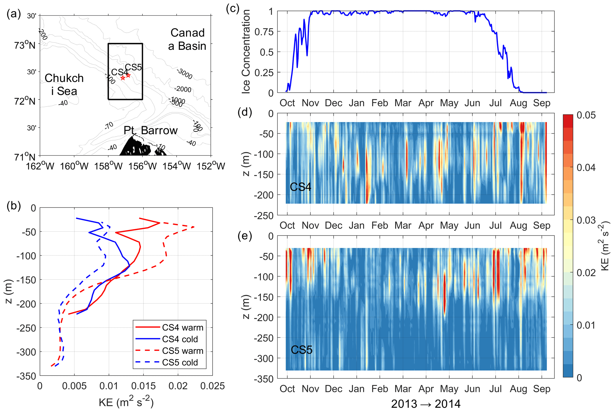
Figure A1 (a) Locations of the BOEM Chukchi slope moorings CS4 and CS5. The black box outlines the region for calculating the ice concentration. (b) Vertical profiles of the KE averaged over warm (October and November 2013 and July to September 2014) and cold (December 2013 to June 2014) months at moorings CS4 and CS5. The warm (cold) month is defined as the month with the mean ice concentration less (larger) than 0.9. (c) Time series of the area-mean ice concentration from October 2013 to September 2014. (d, e) Time–depth plots of the KE at moorings CS4 and CS5.