Assimilation of sea surface salinities from SMOS in an Arctic coupled ocean and sea ice reanalysis

In the Arctic, the sea surface salinity (SSS) plays a key role in processes related to water mixing and sea ice. However, the lack of salinity observations causes large uncertainties in Arctic Ocean forecasts and reanalysis. Recently the Soil Moisture and Ocean Salinity (SMOS) satellite mission was used by the Barcelona Expert Centre to develop an Arctic SSS product. In this study, we evaluate the impact of assimilating this data in a coupled ocean–ice data assimilation system. Using the deterministic ensemble Kalman filter from July to December 2016, two assimilation runs respectively assimilated two successive versions of the SMOS SSS product on top of a pre-existing reanalysis run. The runs were validated against independent in situ salinity profiles in the Arctic. The results show that the biases and the root-mean-squared differences (RMSD) of SSS are reduced by 10 % to 50 % depending on the area and highlight the importance of assimilating satellite salinity data. The time series of freshwater content (FWC) further shows that its seasonal cycle can be adjusted by assimilation of the SSS products, which is encouraging of the assimilation of SSS in a long-time reanalysis to better reproduce the Arctic water cycle.

1 Introduction

The Arctic Ocean is undergoing a dramatic warming, resulting in the loss of sea ice as documented by previous studies (e.g., Johannessen et al., 1999; Stroeve and Notz, 2018). Sea ice melt contributes freshwater to the Arctic Ocean, together with precipitation and river flux, and has far-reaching effects on the Arctic Ocean environment (Carmack et al., 2016). The Arctic observing system, compared to other oceans, lacks the capability to provide a complete picture of ocean salinity, particularly because of obstruction by sea ice. A complete reconstruction of Arctic environmental variables thus requires a data-assimilative numerical model capable of propagating information below sea ice during the winter, as practiced by ocean operational forecast systems (such as Dombrowsky et al., 2009; Fujii et al., 2019). As with other ocean data assimilation (DA) applications, Arctic reanalysis products of ocean and sea ice play an important role in understanding climate change and its mechanisms. In recent years, many studies (e.g., Storto et al., 2019; Uotila et al., 2019) evaluated the quality of the Arctic reanalysis products and recommended experiments to maximize the usefulness of new observations, as done by Kaminski et al. (2015) and Xie et al. (2018). However, there are no impact studies of salinity observations in the Arctic to our knowledge.

Ocean salinity has been used to study the water cycle for the last 20 years (e.g., Curry et al., 2003; Boyer et al., 2005; Yu, 2011; Yu et al., 2017). A recent review paper showed a stabilization of the freshwater content (FWC) in the Arctic Basin, although observations indicate that the Beaufort Gyre keeps getting fresher (Solomon et al., 2021). Salinity variations have far-reaching implications for ocean mixing, water mass formation, and ocean general circulation but suffer from large uncertainties in the Arctic, mainly due to sparse observations and the lack of a steady-state reference time period (e.g., Stroh et al., 2015; Xie et al., 2019). Measuring sea surface salinity (SSS) from passive microwave remote sensing is a comparatively new but promising way to reduce the uncertainty in salinity. Launched in November 2009, the Microwave Imaging Radiometer using Aperture Synthesis (MIRAS) instrument of the European Space Agency's (ESA) Soil Moisture and Ocean Salinity (SMOS) mission measures the brightness temperatures (T_B) of the sea surface at different frequency bins. The passive 2-D interferometric radiometer on the satellite operating in L-band (1.4 GHz) is sensitive to water salinity and is sufficiently free from electromagnetic interference (e.g., Font et al., 2010; Kerr et al., 2010). Since May 2010, SMOS operationally provides SSS records over the global ocean (Mecklenburg et al., 2012). During the last 12 years, large improvements have been introduced in the SMOS data-processing chain, increasing the accuracy and coverage of the salinity data up to levels that were unthinkable at the beginning of the mission (Martin-Neira et al. 2016, Olmedo et al., 2018; Reul et al., 2020; Boutin et al., 2022).

Furthermore, the assimilation of satellite-derived SSS products using an ensemble DA method has been found to significantly improve the surface and subsurface salinity fields in the tropics (Lu et al. 2016). The advantages of assimilating three SSS products from SMOS, Aquarius (ref., Lee et al., 2012), and the Soil Moisture Active Passive Mission (SMAP; e.g., Tang et al., 2017) into a global ocean forecast system using a 3D-Var DA method have also been demonstrated by Martin et al. (2019). Their results show the benefits of assimilating both the SMOS and SMAP datasets in the intertropical convergence zone in the tropical Pacific. However, very few studies have investigated the impact of assimilating SSS products in the Arctic or at high latitudes. Since the beginning, the SSS retrieval from SMOS in cold regions has been very challenging for three main reasons: (i) the lower sensitivity of T_B to salinity in cold waters leads to larger errors (Yueh et al., 2001; e.g, the sensitivity drops from 0.5 to 0.3 K PSU⁻¹ when sea surface temperature decreases from 15 to 5 ^∘C); (ii) land–sea and ice–sea contaminations resulting from abrupt changes of T_B values across these two interfaces, combined with the large ground footprint of SMOS; (iii) the requirement of a well-observed steady-state period for the removal of biases. Addressing these challenges in the SMOS salinity retrieval approach, Olmedo et al. (2017) introduced a non-Bayesian retrieval method to de-bias the Level 1 baseline (L1B) salinity against the reference SSS from Argo data (Argo, 2022). Level 1 data from the satellite are available within 24 h, but the additional processing steps require high-quality auxiliary data, so Levels 3 and 4 SSS are only provided in delayed mode. Starting with the ESA L1B (v620) product from SMOS, the Barcelona Expert Centre (BEC) released version 2.0 of the Arctic gridded SSS product (25 km resolution; Olmedo et al., 2018). Xie et al. (2019) evaluated the V2.0 SSS product and another gridded Arctic SMOS SSS product developed by LOCEAN (Boutin et al., 2018) during the years 2011–2013. These two SSS observation sets, together with an Arctic reanalysis (Xie et al., 2017) and one objective analysis product (Greiner et al. (2021) describe an updated version of this product), were validated against in situ observations and compared with two climatology datasets: the World Ocean Atlas of 2013 (WOA2013; Zweng et al., 2013) and the Polar science center Hydrographic Climatology (PHC 3.0; Steele et al., 2001). They found considerable discrepancies among the different gridded SSS products, especially in the freshest seawater (< 24 psu). The intercomparison of these Arctic SSS products shows room for improvement of the SMOS-based SSS in the Arctic.

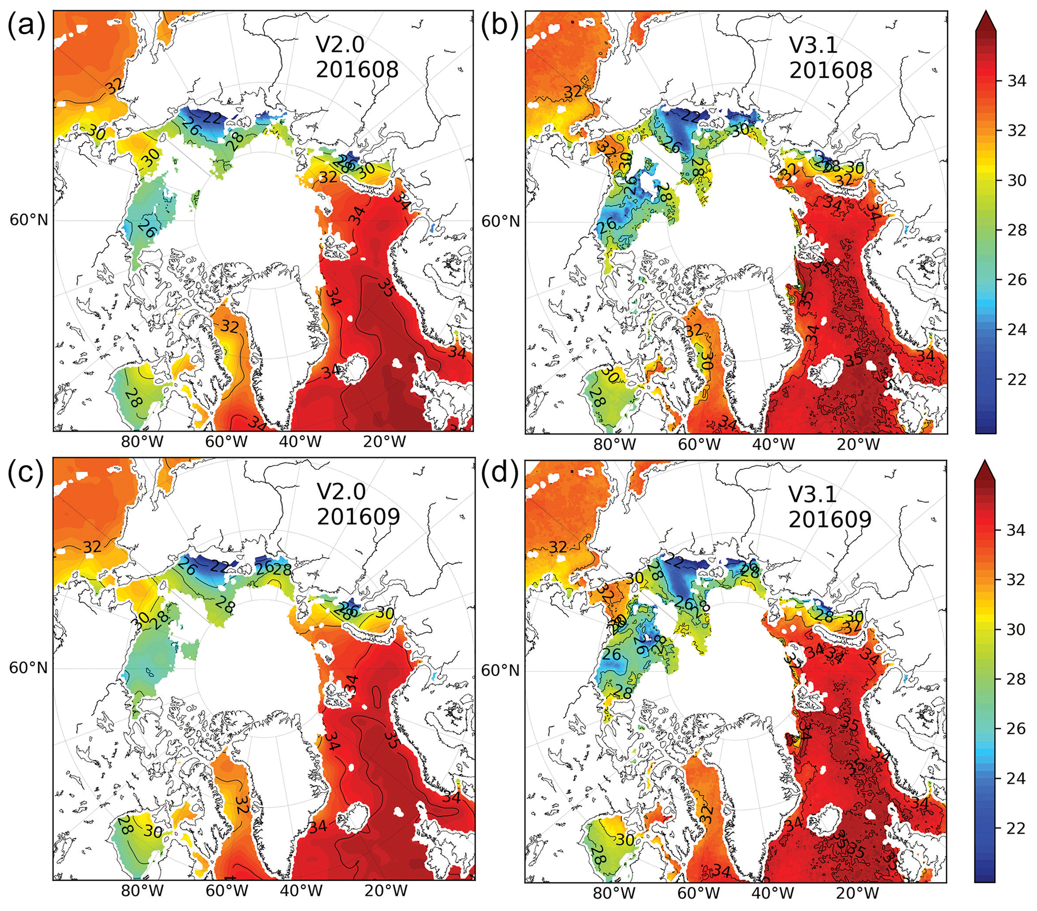
Figure 1 Monthly SSS of August (a, b) and September (c, d) in 2016 from SMOS products of BEC V2.0 (a, c) and V3.1 (b, d). Note: the solid isolines of SSS are 22, 26, 28, 30, 32, 34, and 35 psu.

Recently, under the framework of the ESA project Arctic+Salinity (AO/1-9158/18/I-BG) and further development of the non-Bayesian scheme (Olmedo et al., 2017), the effective resolution of SSS data was enhanced both in space and time (Martínez et al., 2022). The new version of the SSS product (V3.1) has the capability to monitor mesoscale structures and river discharges (e.g., Martínez et al., 2022). This new product provides daily maps (Level 4) of 9 d averages in the Arctic on a regular 25 km grid and covers a longer time period of 2011–2019; these are released through the BEC portal (http://bec.icm.csic.es/ and also at DOI: https://doi.org/10.20350/digitalCSIC/12620; last access: May 2022). The major differences in the estimation of the two SSS products (V2.0 and V3.1) are detailed in the Algorithm Theoretical Baseline Document (ATBD) of the Arctic+Salinity project (Martínez, 2020). Figure 1 shows that, in comparison to V2.0, V3.1 provides wider coverage in the marginal seas around the Arctic and is also fresher, as indicated by the 26 psu isoline.

The two successive versions of the BEC SMOS SSS products are assimilated into the TOPAZ Arctic reanalysis system (detailed in Sect. 2) during the summer of 2016. These two assimilation runs are compared to the Arctic reanalysis without assimilation of satellite SSS data, which is identical to the product ARCTIC_REANALYSIS_PHYS_002_003 in the Copernicus Marine Services. The model validation against independent observations presents the differences stemming from these two SSS products, although they are from the same initial data source (SMOS). Their impact on the assimilation in the Arctic coupled ice–ocean model shows large differences, thereby motivating further efforts to improve SSS retrievals in the cold Arctic.

The paper is organized as follows: Sect. 2 briefly describes the coupled ocean and sea ice data assimilation system and the assimilation experiments; Sect. 3 describes the in situ observations and the validation metrics; results presented in Sect. 4 include the validation using independent SSS observations, separated into different ocean basins. Sect. 4 also examines the impact of SSS assimilation on the weekly increments of other related variables near the surface and explores the integrated effect on the freshwater simulated by the model. In Sect. 5, the findings of this study and future perspectives are summarized.

2 Assimilation system and experimental design

2.1 The Arctic ocean and sea ice coupled data assimilation system

TOPAZ is a coupled ocean and sea ice data assimilation system, built using the deterministic ensemble Kalman filter (DEnKF; Sakov et al., 2012) to simultaneously assimilate multiple types of observations for the ocean and sea ice (Xie et al., 2017). The ocean model in this system uses version 2.2 of the Hybrid Coordinate Ocean Model (HYCOM; Chassignet et al., 2003) with a low-distortion square grid at a horizontal resolution of 12–16 km. The river discharge input is climatological, using the ERA-Interim (Dee et al., 2011) runoffs channeled in a simple hydrological model, which tends to underestimate the amplitude of the seasonal cycle and thus produces a saline bias at the surface (Xie et al. 2019). The coupled sea ice model uses a single-category thermodynamic model (Drange and Simonsen, 1996) and dynamics by the modified elastic–viscous–plastic rheology (Bouillon et al., 2013) from an early version of the CICE model (Lisæter et al. 2003). The model covers the Arctic Ocean and the whole north Atlantic Ocean (shown in Fig. 1 in Xie et al., 2017). A seasonal inflow of Pacific Water is imposed across the Bering Strait, based on observed transports (Woodgate et al., 2012). At all lateral boundaries, the temperature and salinity stratifications are relaxed to a climatology combining version 2.0 of WOA2013 and version 3.0 of PHC with a 20-grid-cells buffer zone. To avoid a potential model drift, the surface salinity is relaxed to the combined climatology as mentioned above, with a 30 d timescale, but the relaxation is suppressed wherever the difference from climatology exceeds 0.5 psu to avoid the artificial formation of bulk surface freshwater layers.

For simplification, the two steps of the assimilation system can be translated by the following concept expressions (update and model propagation):

$$\begin{array}{}\text{(1)}& {\displaystyle }{\mathbf{X}}_{\mathrm{a}}={\mathbf{X}}_{\mathrm{f}}+\mathbf{K}(\mathit{y}-H{\mathbf{X}}_{\mathrm{f}}),\text{(2)}& {\displaystyle }{\mathbf{X}}_{\mathrm{f}}=M\left({\mathbf{X}}_{\mathrm{a}}\right),\end{array}$$

where the matrix X represents the model state with all 3-D and 2-D variables needed by the model forward integration, represented by the operator M. The subscripts “a” and “f” respectively indicate the analyzed model state obtained through optimization after DA and the model forecast. The vector y is composed of the quality-checked observations during the weekly cycle, and the observation operator H gives the model equivalent of the observations. The innovation term (in parentheses in Eq. 1) represents the differences between the model and the various observations in the observation space.

For the ensemble data assimilation method, the matrix X includes the dynamical members of the model states as different columns and further evolutes according to Eqs. (1) and (2), as described in the DEnKF. The TOPAZ model runs an ensemble of 100 members. The K matrix (Kalman gain) is calculated using the ensemble covariance matrix. Like other square root versions of the ensemble Kalman filter, the DEnKF splits Eq. (1) into two steps: the K calculation is applied to the ensemble mean, and the anomalies are updated to match a target analysis covariance (more details in Sakov et al., 2012). Using a 7 d assimilation cycle, we use the DEnKF to assimilate different types of ocean and ice observations, including along-track sea level anomaly (SLA), sea surface temperature (SST), in situ profiles of temperature and salinity, sea ice concentrations (SIC), and sea ice drift products all sourced from the Copernicus Marine Environment Monitoring Services (CMEMS; https://marine.copernicus.eu, last access: February 2023). The same TOPAZ system provides a 10 d forecast of ocean physics and biogeochemistry in the Arctic (Bertino et al., 2021) every day via the CMEMS portal.

Table 1 Settings of the three assimilation runs in 2016 with and without SSS.

n/a: not applicable.

2.2 Assimilation experiments and the observation error estimate for SSS

To evaluate the impact of the assimilation of two versions of the SSS products on TOPAZ model runs, a control assimilation experiment (Exp0) and two parallel assimilation experiments (ExpV2, ExpV3) for a 6 month time period (July to December 2016) were performed. Exp0 assimilates all available ocean and sea ice data, except the satellite SSS products. On the other hand, ExpV2 and ExpV3 additionally assimilate the BEC SSS products V2.0 and V3.1, respectively. Details of the three assimilation runs are listed in Table 1.

Observation error is a key parameter in any DA system: too-small values lead to overfitting, while too-large values make the assimilation inefficient. The salinity errors from passive microwave instruments were previously estimated by Vinogradova et al. (2014): the zonal average of standard errors north of 60^∘ N was estimated at 0.6 psu. In a recent study, Xie et al. (2019) evaluated the SMOS-based SSS products using in situ observations and revealed a strong regional dependence of the V2.0 product errors: they are smaller than 0.4 psu in the Northern Atlantic but increase dramatically to 1 psu in the Nordic seas and to over 2 psu in the central Arctic. Undoubtedly, the salinity observation errors from passive microwave instruments are higher in high latitudes than they are elsewhere. Furthermore, in the Beaufort Sea (as Fig. 12a in Xie et al., 2019), the errors of the SSS V2.0 product and the Arctic reanalysis product from TOPAZ (same as Exp0 used in this study) both show an inverse relationship between SSS values and SSS errors. Hence, we use an empirical error function for ExpV2 and ExpV3 adjusted to the discrepancies as shown in Eq. (3), following Xie et al. (2019):

$$\begin{array}{}\text{(3)}& E_{\text{SSS}}=\text{max}\left\{E_{\text{int}},{\left[\mathrm{0.6}+{\displaystyle \frac{\mathrm{6}}{\mathrm{1}+\text{exp}\left(\frac{\text{SSS}-\mathrm{16}}{\mathrm{5}}\right)}}\right]}^{\mathrm{2}}\right\},\end{array}$$

where E_int is the instrumental error variance estimated by the data provider – that part is absent from the V2.0 product. Equation (3) yields more conservative error estimates than the providers, which also prevents the discontinuities caused by strong assimilation updates (as an example noticed by Balibrea-Iniesta et al., 2018). The settings for all other observation types are identical to those applied in Xie et al. (2017). By construction, the observation errors are always larger for the V3.1 than for the V2.0 product, but in fresh waters they are identical. This implies that the assimilation may pull the analysis closer to the V2.0 than to the V3.1 product in the more saline waters, but they are otherwise treated on equal footing, ignoring the a priori expectation that the most recent product should be more reliable.

Figure 2 Locations of the observed SSS from in situ profiles and surface samples by cruises from July to December 2016. The marks note six observation sources; see the details in Sect. 2.3. The marginal seas delineated are the Beaufort Sea (BS), Chukchi Sea (CS), East Siberian Sea (ESS), Laptev Sea (LS), Kara Sea (KS), Barents Sea (BSS), Greenland Sea (GS), Norwegian Sea (NS), and Baffin Bay (BB). The main rivers around the Arctic region are the Mackenzie River (MR), Pechora River (PR), the Ob (OB), Yenisey River (YR), Lena River (LR), and Indigirka River (IR). TP indicates the Taymyr Peninsula.

3 In situ SSS observations for validation

All in situ salinity profiles were collected from various repositories and cruises (as shown in Fig. 2). Salinity measurements were extracted near the surface over the Arctic domain during the experimental time period. The sanity check procedures include the following: (i) location check to remove SSS observations in the model land mask; (ii) omission of the invalid profiles if the top depth is deeper than 8 m; (iii) removal of the redundant observations. Since the model does not reproduce local gradients of the vertical salinity profiles shown in Supply et al. (2020), all the salinity profiles are averaged over the upper 8 m below the surface. This also avoids the loss of the profiles that do not reach the surface.

• Data from the Beaufort Gyre experiment project (BGEP).

  The BGEP has maintained an observing system in the Canadian Basin since 2003 and provides in situ observations over the Beaufort Gyre every summer. Although the BGEP has maintained three bottom-tethered moorings since 2003, the shallowest depth of the measured profiles for temperature and salinity is below 50 m. Hence, in this study, we only use the conductivity temperature depth (CTD) dataset from the cruise in 2016 (https://www2.whoi.edu/site/beaufortgyre/data/ctd-and-geochemistry/, last access: 14 February 2022). SSS observations from these CTD profiles in the time period from 13 September to 10 October 2016 are represented by the red triangles in Fig. 2.

• Data from Oceans Melting Greenland (OMG).

  The project Oceans Melting Greenland was funded by NASA to understand the role of the ocean in melting Greenland's glaciers. Over a 5 year campaign, this project collected temperature and salinity profiles by Airborne eXpendable Conductivity Temperature Depth (AXCTD) launched from an aircraft (e.g., Fenty, et al., 2016). The deployed probe can sink to a depth of 1000 m, connected with a float by a wire. The measured temperature and conductivity are then sent back to the aircraft. These salinity profiles collected during the first OMG campaign in 2016 are downloaded from https://podaac.jpl.nasa.gov/dataset/OMG_L2_AXCTD/ (last access: 10 February 2022). The SSS from OMG distributed around Greenland from 13 September to 10 October 2016 is shown as the inverted blue triangles in Fig. 2.

• Data from the International Council for the Exploration of the Sea (ICES).

  Salinity profiles were also obtained from the ICES portal (https://www.ices.dk, last access: November 2022). Shown as light-blue squares in Fig. 2, the locations of the profiles during the last 6 months of 2016 are dense in the Nordic Seas and are restricted to north of 58^∘ N for this study. Valid salinity profiles from ICES (last access: 9 February 2022) are obtained from 6 July to 23 November in 2016.

• Data from other cruises at the Arctic Data Center (ADC).

  Surface salinity observations from scientific cruises are obtained from the Arctic Data Center portal (https://arcticdata.io/catalog/data; last access: 17 February 2022). During the model experiment, the first relevant cruise in ADC was SKQ201612S, which was operated by University of Alaska Fairbanks with the RV Sikuliaq. This cruise collected data from Nome, Alaska, on 3 September 2016, heading to the northeast Chukchi Sea and then back to Nome at the end of September 2016. The temperature and salinity profiles were collected by a Sea-Bird 911 CTD instrument package. All measurements at each station were done both down- and upcast-ways. To produce water column profiles at each station, the downcast data were binned at 1 m intervals (Go ni et al., 2021). Besides the CTD profiles of SKQ201612S, more seawater samples were collected via the surface underway system on the RV Sikuliaq. Through a sea chest below the waterline (e.g., 4–8 m), the uncontaminated seawater was pumped into the ship, and the corresponding filtration system supplied samples every 3 h to the sensors (More details in Go ni et al., 2019). These SSS observations were obtained on 9–27 September, indicated as blue crosses in Fig. 2.

Moreover, SSS measurements were also collected from the Sea-Bird CTD on board Sir Wilfrid Laurier (SWL) but only in July 2016. This cruise is part of the annual monitoring from the Canadian Coast Guard Service (Cooper et al., 2019). The SSS observations are obtained near the Bering Strait, close to the Pacific boundary of our model.

After filtering the diurnal signals by daily averages in observed surface salinity, all valid SSS measurements from the above data sources are compared with the daily average SSS of the three assimilation experiments listed in Table 1. The model data have been collocated with the observations for validation. To estimate the forecast differences to observations, we use the standard statistical moments:

$$\begin{array}{}\text{(4)}& {\displaystyle }\text{Bias}={\sum }_{i=\mathrm{1}}^N{\sum }_{\mathrm{1}}^{O_i}\left(H{\stackrel{\mathrm{‾}}{\mathbf{X}}}_i-{\mathit{y}}_i\right)/{\sum }_{i=\mathrm{1}}^N{O}_i,\text{(5)}& {\displaystyle }\text{MSD}=\sqrt{{\sum }_{i=\mathrm{1}}^N{\sum }_{\mathrm{1}}^{O_i}{\left(H{\stackrel{\mathrm{‾}}{\mathbf{X}}}_i-{\mathit{y}}_i\right)}^{\mathrm{2}}/{\sum }_{i=\mathrm{1}}^N{O}_i},\end{array}$$

where i is the ith day, O_i represents the number of observations on this day, and N represents the total number of days depending on the source of observations. Then ${\stackrel{\mathrm{‾}}{\mathbf{X}}}_i$ represents the model daily average of the ensemble mean at the observation time. H is an operator to extract the SSS simulation from the model at the observed location. The model performance can then be quantitatively compared between the three assimilation runs.

In addition, we further introduce a two-sample Student's t test to evaluate the significance of the change of SSS bias in ExpV2 and ExpV3 with respect to Exp0. Compared to in situ observations, the SSS misfits in Exp0 are the error array e₁. The corresponding error array from ExpV2 or ExpV3 is called e₂. Thus, considering the null hypothesis H0 that ${\stackrel{\mathrm{‾}}{e}}_{\mathrm{1}}$ and ${\stackrel{\mathrm{‾}}{e}}_{\mathrm{2}}$ are the means of indiscernible random draws, the t value can be calculated as follows:

$$t={\displaystyle \frac{\left|{\stackrel{\mathrm{‾}}{\mathbf{e}}}_{\mathrm{2}}-{\stackrel{\mathrm{‾}}{\mathbf{e}}}_{\mathrm{1}}\right|}{\sqrt{s_{\mathrm{1}}^{\mathrm{2}}/(n_{\mathrm{1}}-\mathrm{1})+s_{\mathrm{2}}^{\mathrm{2}}/(n_{\mathrm{2}}-\mathrm{1})}}},$$

where s₁ (s₂) is the standard deviation in the e₁ (e₂), and n₁ (n₂) is the number of observations. For every t value, the p value from the above equation is the probability that random errors would prove H0 wrong. Low p values (< 0.05) indicate that the change of bias due to assimilation is significant.

Figure 3 Innovation statistics of SSS in the Arctic (> 60^∘ N) from ExpV2 (a) and ExpV3 (b). The line with red triangles is the root-mean-squared innovation, and the dotted blue line shows the mean of innovations north of 60^∘ N. The gray line represents the number of observations assimilated, and the green line with inverted triangles is the observation error standard deviation in the two runs.

4 Results

4.1 Diagnosing using assimilation statistics

The SSS innovations in the two assimilation runs of ExpV2 and ExpV3 are compared in Fig. 3, together with the number of assimilated SSS observations and the ensemble spread calculated by the ensemble standard deviation. The total number of observations is at its maximum in September, when the sea ice cover is minimal. Since both versions of the SSS product share the same time frequency (9 d average) and gridded format, the number of assimilated observations in the two runs reached a maximum in the middle of September (gray lines in Fig. 3). But the maximal number of SSS in ExpV3 is shown to be higher than in ExpV2. For ExpV2, the root mean square (RMS) of the SSS innovation varies between 0.4 and 1.2 psu, but the mean of SSS innovation, calculated as the observation minus the model simulation (see the bracket in Eq. 1), shows a saline bias of 0.4 psu, highest in September. However, in ExpV3, the salinity bias quickly disappears after a few data assimilation cycles. The RMS of the SSS innovation is larger in ExpV3 between 0.6 and 1.6 psu, which can partly be explained by the higher effective resolution of the V3.1 product and the double-penalty effect. In ExpV3, the RMS of the SSS innovation (the red line) jumps down after the first SSS assimilation step. The RMS of SSS innovations and the observation errors both decrease from summer to winter, following a seasonal cycle as the areas of fresher water get gradually ice covered. The domain-averaged observation errors are only slightly larger in ExpV3 than in ExpV2, as explained above, and the RMS of SSS innovations becomes lower than the observation errors near the end of the run, which indicates that the observation errors for the V2.0 SSS have been overestimated.

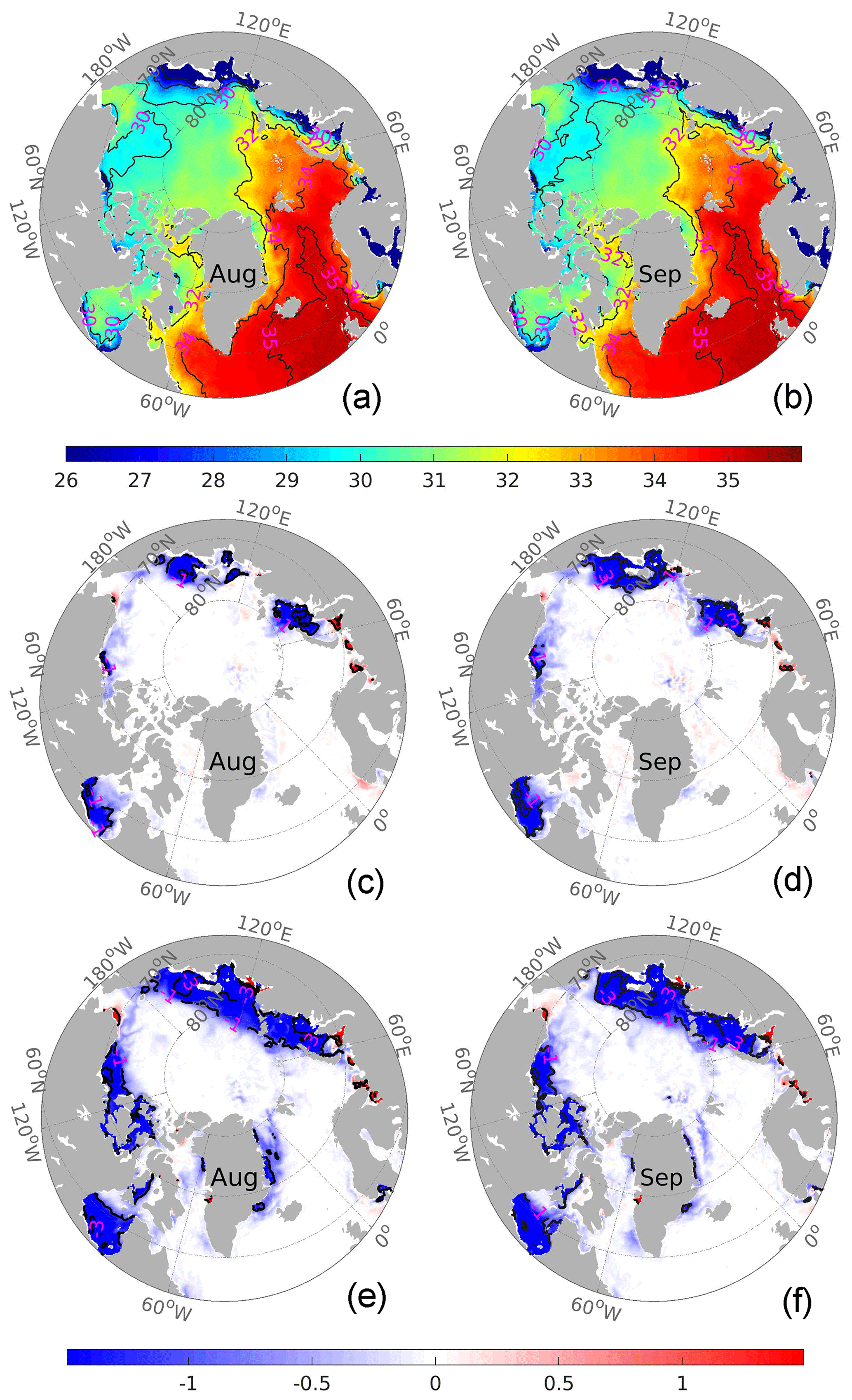
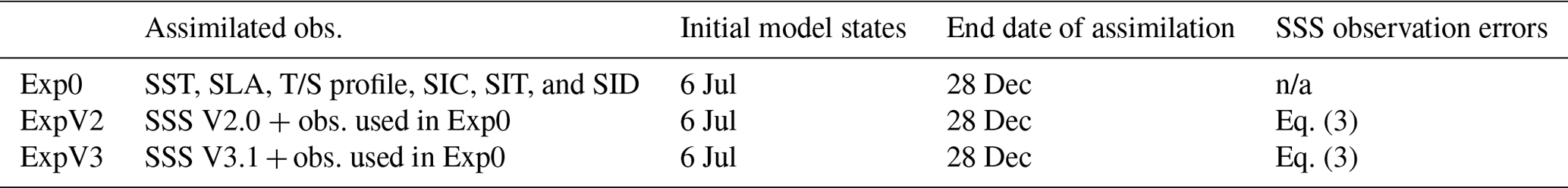
Figure 4 (a, b) Monthly simulated SSS (unit: psu) from Exp0 in August (a) and September 2016 (b). The black isolines indicate the 26, 28, 30, 32, 34, and 35 psu, respectively. (c–f) Monthly SSS differences in ExpV2 (c, d) and ExpV3 (e, f) with respect to Exp0. The black lines are −3, −1, 1, and 3 psu.

In Fig. 4a and b, the SSS maps are shown for the control run (Exp0) in August and September 2016, respectively. For Exp0 in August, low-salinity waters are found in the Beaufort Sea near the Mackenzie River and along the East Siberian coast. In September, the fresher waters, below 30 psu, bridge the two areas in Exp0, probably due to sea ice melt, although the lowest salinity near the Siberian coast remains unchanged from August to September (as indicated by the 28 psu isoline). Compared with the SSS observations from SMOS (Fig. 1), these two low-salinity waters are clearly underestimated in Exp0. Meanwhile, the relatively saline 32 psu isoline crosses both the Eurasian Basin and Baffin Bay. In the Laptev Sea, due to the significant effects of river runoff and ice melt, the salinity shows a strong gradient from the southeast to the northern part. During winter, the salinity increases to 34 psu, and it decreases in summer to nearly 30 psu (Janout et al., 2017). In the northwest Laptev Sea, the saline tongue of 32 psu extends eastward to the Taymyr Peninsula (TP). North of the TP, the Kara Sea freshwater meets with the Atlantic Water pathways from the Fram Strait and Barents Sea (shown in Fig. 1 of Janout et al., 2017). Close to the TP, the observations at the mooring profiles in Janout et al. (2017) show much fresher surface salinity (29 psu) than the subsurface salinity (32 psu) in summer. Compared to the SMOS SSS maps (shown in Fig. 1), only the V3.1 product shows the 32 psu isolines around the TP. Another difference between the two SMOS products arises in the Chukchi Sea, where the V3.1 product is more saline than both the V2.0 product and SSS in Exp0.

Figure 4c–f shows the SSS differences in August and September 2016 between the SSS assimilation runs and the control run. Figure 4c and d both show a freshening of the coastal areas in the Kara Sea, Laptev Sea, and East Siberian Sea, but in ExpV3 the freshening is stronger and wider (Fig. 4e and f). In the Beaufort Sea, ExpV2 mainly brings a local freshening near the mouth of the Mackenzie River in August, which then spreads out along the coast in September. The freshening in the BS brought by ExpV3 affects a broader area, even including the Canadian Archipelago. ExpV3 also freshens the SSS on both sides of Greenland Island. From August onwards, the SSS in ExpV3 freshens by over 1 psu along the whole east Greenland coast, which clearly does not happen in ExpV2. In fact, the 32 psu isoline in ExpV3 (not shown) extends hundreds of kilometers further to the southeast Greenland coast in comparison to Exp0 and ExpV2. The rest of the Greenland coast is also fresher by 0.5 psu in ExpV3 during both months. This is a sign of a consistent change in the V3.1 product.

Even though most of the SSS assimilation leads to a freshening of the surface, a few locations show higher salinity than Exp0, these are different from ExpV2 to ExpV3. For example, the saline increment near the Bering Strait is larger in ExpV3 in excess of 1 psu, consistently with the difference between the two remote sensing products (Fig. 1).

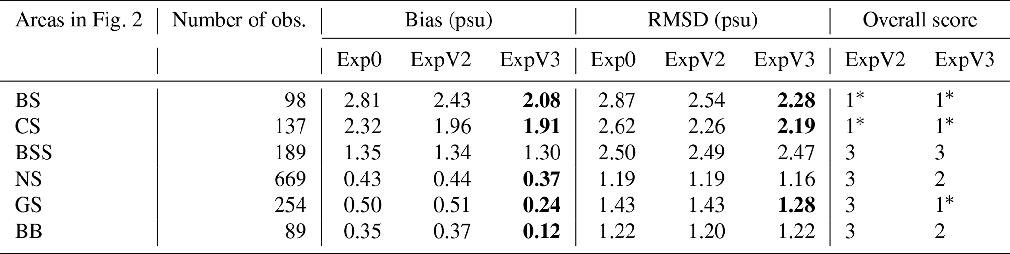
Table 2 Evaluation of SSS misfits (unit: psu) in the three assimilation runs according to the six areas indicated by the dashed blue lines in Fig. 2. The numbers in bold indicate the smallest misfit, with a reduction of at least 9 % relative to Exp0. The overall score depends on whether the bias and RMSD are reduced by at least 9 %. If both criteria are met, the score equals 1; it is 2 if only one of them is met, and it is 3 otherwise. The ^∗ subscript means the bias changes passed the significance test using Student's t test (α = 0.05).

Other increases in SSS concern small areas near estuaries and are more common in ExpV3. The increase to the west of the Yamal Peninsula can be explained by a model setup bias in the location of the Ob river but is compensated for by the SSS assimilation. In the above comparisons of SSS maps, the central Arctic is not discussed, since the region is covered by sea ice and the effect of assimilation is indirect.

4.2 Comparison with independent in situ observations

Quality-checked in situ observations in the central Arctic are very unevenly distributed. After pooling all platforms together, we further investigate the SSS misfits in six subregions of the Arctic (Fig. 2 and Table 2). This section will present the statistics of differences to independent in situ observations, separately considering marginal seas.

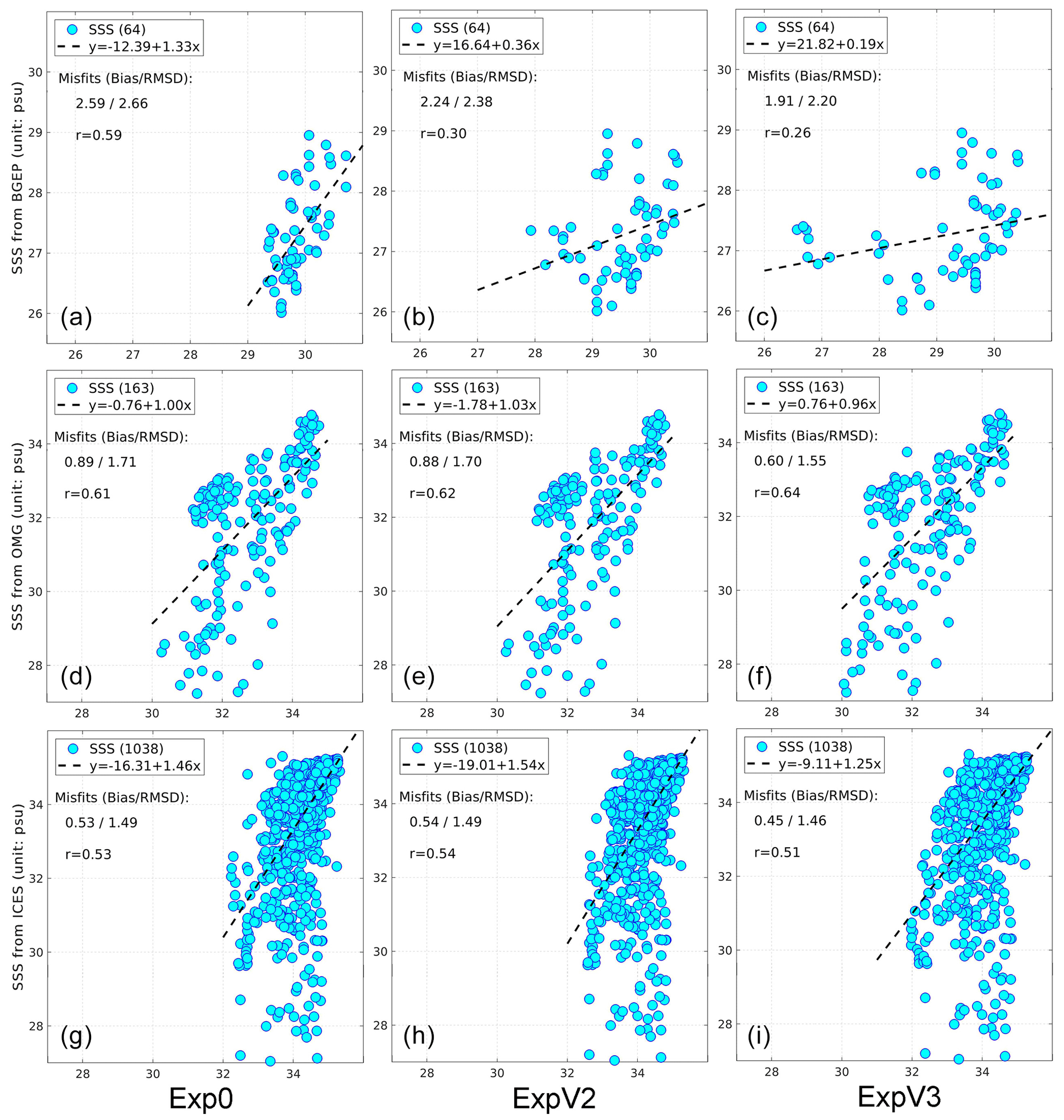
Figure 5 Scatterplots of SSS in the TOPAZ assimilation runs against in situ profiles (top: from BGEP in the Beaufort Sea; middle: from OMG in both Greenland seas; bottom: from ICES in the Nordic Seas, as indicated in Fig. 1 and descriptions in Sect. 3). The statistics of SSS misfits are indicated in each panel with the bias and the RMSD, respectively; the number of observations is given between parentheses. The dashed dark line represents the linear regression, and r is the linear correlation coefficient. All the correlation coefficients are over the 95 % significance test.

Beaufort Sea (BS). Figure 5 shows the scatterplots of SSS in the three runs against in situ observations from BGEP, OMG, and ICES. In the Beaufort Sea (Fig. 5a–c), the observed SSS varies in a range of 26–29 psu. The range of SSS in Exp0 is much smaller, between 29–31 psu, with a saline bias of 2.6 psu and an RMSD of 2.7 psu, but otherwise, it shows a reasonably linear relationship (r=0.59). The SSS bias in Exp0 has the same value as in Xie et al. (2019), although it is estimated using the BGEP observations in a different time period (2011–2013). The range of SSS in ExpV2 is slightly improved to 28–30.5 psu. Further, the bias is reduced by 0.5 psu, corresponding to bias and RMSD reductions of, respectively, 13.5 % and 10.5 % with respect to Exp0. In ExpV3, the SSS range is much closer, between 26.5 and 30.5 psu, and the resulting bias and RMSD reductions of SSS are, respectively, 26.3 % and 17.3 % with respect to Exp0. Both the bias reductions in ExpV2 and ExpV3 relative to Exp0 pass the significance test (α = 0.0) through Student's t test. Furthermore, compared to all in situ SSS in BS (Fig. 7a–c), the SSS misfits in ExpV3 show a stronger reduction by 26.0 % for bias and 20.6 % for RMSD. ExpV2 reduces these errors by half as much (13.5 % for bias and 11.5 % for RMSD). These results clearly indicate that the new version of the SSS is more beneficial for data assimilation in the Beaufort Sea.

Chukchi Sea (CS). Figure 6 shows the SSS deviations as a function of time during the SKQ cruise route. Figure 6a shows the surface levels from CTDs. The saline bias (2.8 psu) is more pronounced than in the Beaufort Sea, which we attribute to the proximity to the model boundary in the Bering Strait, relaxed to climatological values, where the interannual variability of Pacific water is not included. After assimilating SSS products, a reduction of the bias is observed during September: by 15.5 % in ExpV2 and up to 22.2 % in ExpV3. The comparison to underway surface water samples (Fig. 6b) also shows an error reduction of around 15 %, though there are fewer differences between ExpV2 and ExpV3.

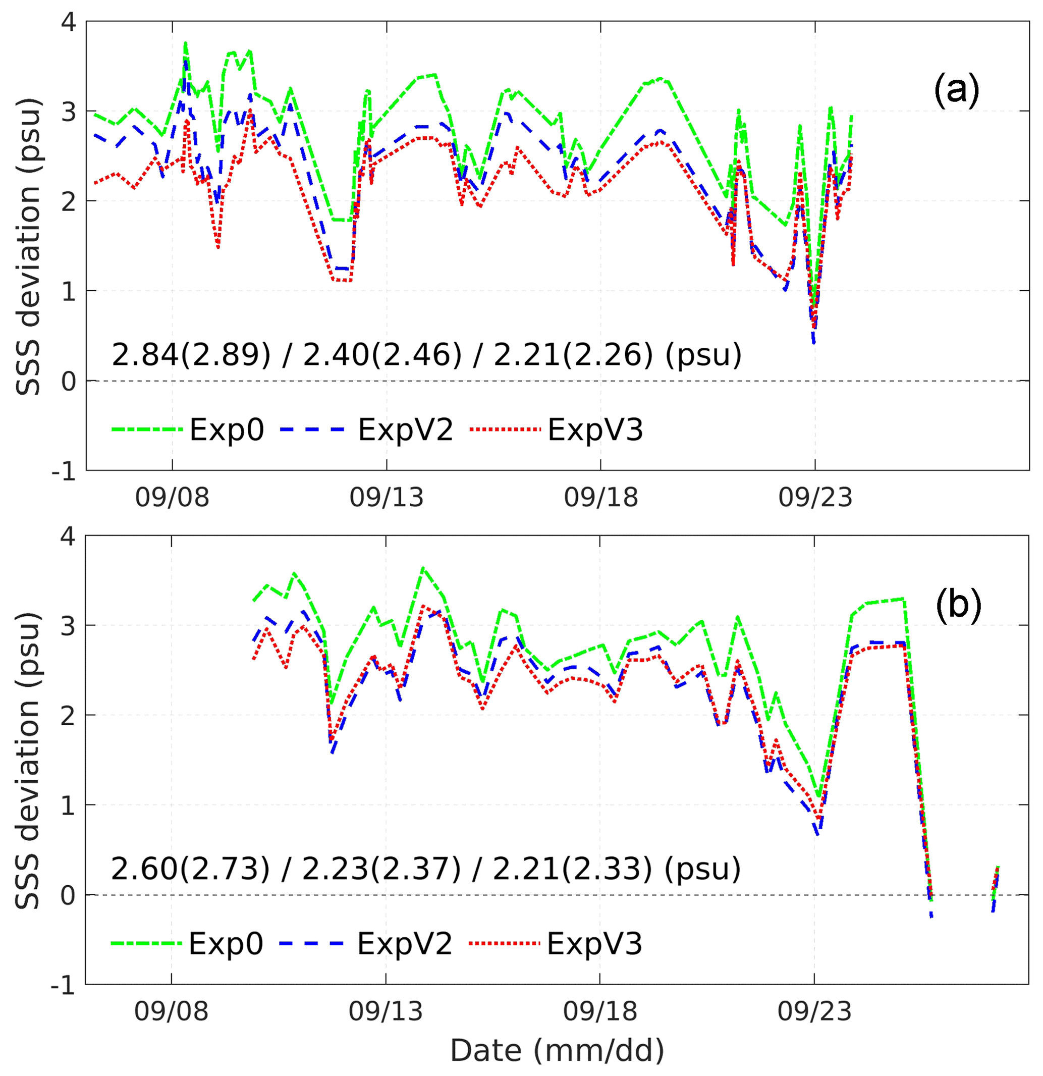
Figure 6 Model-minus-observations SSS differences in the three assimilation runs against the SSS recorded in the Beaufort Sea and the Chukchi Sea along the SKQ cruise in 2016: (a) from CTD profiles; (b) from surface water samples underway in the same cruise. The biases are indicated in the same order, and the corresponding RMSD are between parentheses.

Figure 7 Scatterplots of SSS (unit: psu) in the three assimilation runs Exp0, ExpV2, and ExpV3 against the CTD observations collected by different cruises in 2016. (a–c) Beaufort Sea; (d–f) Chukchi Sea, as shown in Fig. 1. All the correlation coefficients are over the 95 % significance test.

Considering other cruise data in the CS (Fig. 7d–f), the SSS in Exp0 shows almost uniform values, with a saline bias of about 2.3 psu and an RMSD of 2.6 psu. A recent observational study by Goñi et al. (2021) shows that the surface salinity of the CS during late summer varies between 28–30 psu during the time period 2016–2017. The range of SSS observations considered here is slightly broader (27–32 psu). The assimilation of SSS products reduces the misfits (bias and RMSD). As in the BS, the SSS in ExpV3 has more significant reductions in bias (17.7 %) and RMSD (16.4 %). After assimilation, the deviations are in the same range as that found in the BS. All the bias reductions in ExpV2 and ExpV3 are significant compared to Exp0 through the t test (α = 0.05).

Greenland Sea (GS). Most SSS observations around Greenland are from the OMG program, shown as the downward blue triangles in Fig. 2. Considering first all SSS observations from OMG, the SSS misfits in the three runs (shown in Fig. 5d–f) show smaller bias and RMSD than in the BS and the CS. However, the SSS in ExpV3 still brings significant error reductions, with reductions of 32.6 % and 9.4 % of the bias and RMSD compared to Exp0. Notably, the SSS misfits in ExpV2 are almost identical to those in Exp0, which indicates that the V2.0 SSS product was not informative there.

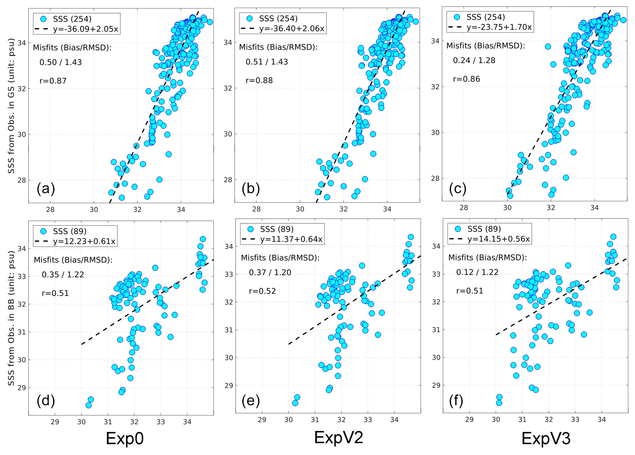
Figure 8 Scatterplots of SSS (unit: psu) in the three assimilation runs Exp0, ExpV2, and ExpV3 against CTD observations from OMG and ICES in 2016. (a–c) East Greenland Sea; (d–f) Baffin Bay, as shown in Fig. 1. The statistics of SSS misfits are indicated in each panel with the bias and the RMSD, respectively, and the number of observations is given between parentheses. The dashed dark line represents the linear regression, and r is the linear correlation coefficient. All the correlation coefficients are over the 95 % significance test.

We now separate the evaluation into the east and west of Greenland, covering the GS and Baffin Bay (BB) areas, as shown in Fig. 2 (also listed in Table 2). Figure 8a–c shows that all SSS observations available in the GS vary between 27 and 35 psu. This large range includes fresh coastal waters, Arctic water, and Atlantic Water. The three assimilation runs show different saline biases, especially for salinities lower than 30 psu. While in observations the minimum salinity is below 28 psu, it only reaches 30 psu in ExpV3 and 31 psu in both Exp0 and ExpV2. As a result, the bias reduction in ExpV3 is over 50 %, and the RMSD decreased by about 10.5 % in the GS. ExpV2 is disappointingly similar to Exp0. This is also the case in BB (shown in Fig. 8d–f), where differences between ExpV2 and Exp0 are less than 0.02 psu. In contrast, ExpV3 reduces the SSS bias but does not significantly reduce the RMSD in the BB. One possible explanation is the double-penalty effect because the V3.1 product has a higher effective resolution than V2.0. This can be seen in Fig. 8, as the ExpV3 values are more scattered.

Finally, we examine the SSS deviations in the Barents Sea and the Norwegian Sea. The SSS bias and RMSD are the lowest in ExpV3 in Table 2, even though the reductions are not as significant as in the area of fresher surface waters. Compared to the ICES observations distributed in the North Atlantic and the Nordic Seas (blue squares in Fig. 2), the scatterplots of Exp0 and ExpV2 are nearly identical (see Fig. 5g–i). The minimum salinity in these two runs is 32 psu. The SSS bias and RMSD in both runs are also similar (differences less than 0.01 psu). In contrast, lower salinity values (below 32 psu) are found in ExpV3, although the saline bias remains around 0.5 psu on average. Notably, the SSS in ExpV3 shows that data assimilation can reduce the bias by 15 % compared to Exp0, but the RMSD only reduced by about 0.03 psu, which is also possibly due to the double-penalty effect. This also suggests that the improvements near the coast will be the next challenge for future versions of the SSS product.

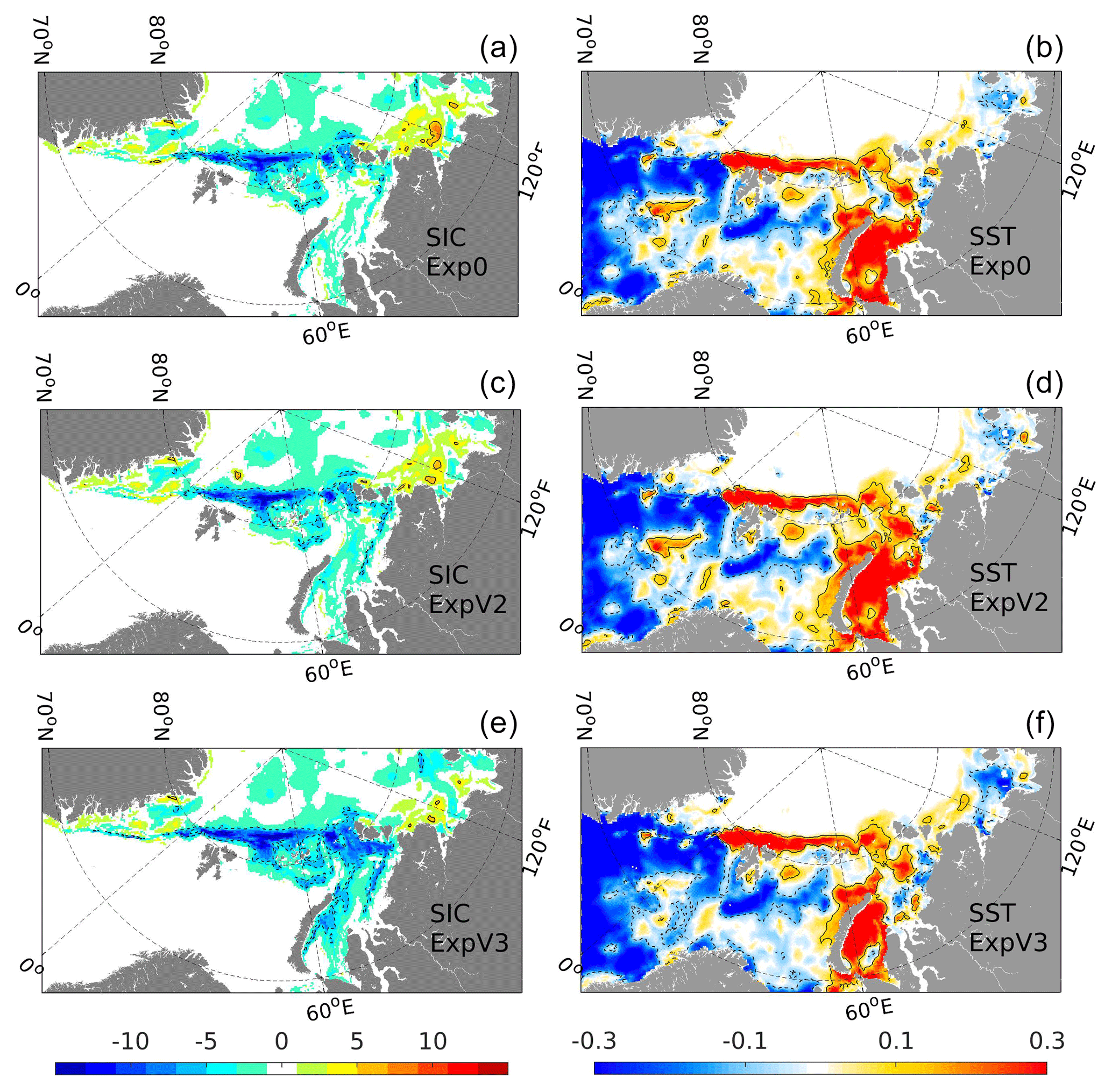
Figure 9 Averaged increments for the 6 month period (a, b in Exp0; c, d in ExpV2; e, f in ExpV3). The figure shows the European Arctic for clarity. (a, c and e) Sea ice concentration (unit: %) with isolines of ± 5 %. (b, d and f) SST with isolines of ± 0.1 ^∘C.

4.3 Impact analysis of SSS assimilation

The above section has demonstrated that the assimilation of remote-sensing SSS generally improves the match to independent in situ measurements, although the improvements are location dependent. Since large areas are void of in situ measurements, the increment for other surface variables will also be interpreted for understanding the impacts incurred. The increments are the differences between the analysis and the forecast. The calculation of them is the result of the innovations of all assimilated observations multiplied by the Kalman gain, as computed in Eq. (1). Since the DEnKF update is multivariate, we present the impact of the assimilation on other model variables closely related to the SSS: SST and SIC. Since the only difference in the setting between the three runs is the assimilation of SSS, we can attribute the differences to the impact of SSS observations. In theory, if both the model and observations were unbiased, the increments of other assimilated variables should generally decrease because of the presence of a new SSS term in the denominator of the Kalman gain (the ensemble covariance matrices contain off-diagonal blocks of correlation between SSS and dynamically related variables, and so the assimilated observations usually compete with each other). However, the SSS biases originating either from the model or observations also affect the other model variables and increase the innovations on the following assimilation step and thus the consecutive increments. Hypothetically, wherever the forecast errors are caused by SSS errors, the increments of other variables should diminish. Figure 9 compares the time-averaged increments of SIC and seawater temperature in the top 3 m layer (considered as SST here) in the three runs. The sign of the increments remains overall the same across the three experiments, both for SST and SIC. The SST increments in the three runs are negative in the open ocean and positive near the ice edge, as shown in the right column of Fig. 9.

The SST increments in Exp0 and in ExpV2 are nearly identical, but in ExpV3 there are a few areas such as in the Kara Sea and in the Laptev Sea where the SST increments have been suppressed. These are locations where the SSS and SST are positively correlated, so the updated SSS by assimilation is also helpful in reducing the water temperature misfits near the surface. The changes in SST are, however, small with respect to the large SSS differences in Fig. 4. In Exp0, the SIC increments are small (< 5 %) inside the ice pack. The satellite SIC observations are assimilated every week and help to correctly position the ice edge (Sakov et al., 2012). The increments exceed 5 % along the ice edge, as can be seen in the northern Barents Sea.

The assimilation of the V2.0 SSS product also shows minimal differences from Exp0, partly because of the conservative sea ice mask in the V2.0 SMOS SSS. The SIC increments are opposite to those of SST, showing that the assimilation warms the surface water where ice is removed, which is consistent with Lisæter et al. (2003). Only minor differences between ExpV2 and ExpV0 are visible along all areas swept by the ice edge during the 6 month experiment, for example in the Kara Sea. In contrast, the assimilation of the V3.1 SSS product shows larger changes in SIC increments than in ExpV2, with a broader area of negative increments (removed ice) in the northern Barents Sea. This is not visibly related to the SST increments but to the freshening caused by the assimilation of V3.1 SSS, as SSS and SIC are positively correlated in the northern Barents Sea, as shown by Fig. 2 in Sakov et al. (2012). The increased SIC increments may be an indication that the SSS freshening could be excessive.

Since the whole water column is updated by assimilation, the freshwater content is also modified by the assimilation of SSS. There are, however, complex relationships between SSS and FWC, as shown by Fournier et al. (2020). The changes in FWC in the Arctic are calculated as in Eq. (6) derived from Proshutinsky et al. (2009), although this method was initially intended for the Beaufort Sea. Applying the same formula for interpolation of in situ observations, Proshutinsky et al. (2020) estimated the time-averaged summer freshwater content in the Beaufort Gyre region in two time periods (1950–1980 and 2013–2018). In the latter period, they located the FWC center in the Beaufort Sea around (150^∘ W, 75^∘ N) and drew the 20 m isoline over more than 5^∘ of latitude and nearly 30^∘ of longitude on average. When compared to the earlier reference period, the FWC in the Beaufort Sea has increased, and its center has shifted westward.

Following Proshutinsky et al. (2009), the model FWC in the Arctic is estimated as follows:

$$\begin{array}{}\text{(6)}& \text{FWC}={\int }_{z_{\mathrm{0}}}^{z_{\text{ref}}}\left(\mathrm{1}-{\displaystyle \frac{S_{\left(z\right)}}{S_{\text{ref}}}}\right)\mathrm{d}z,\end{array}$$

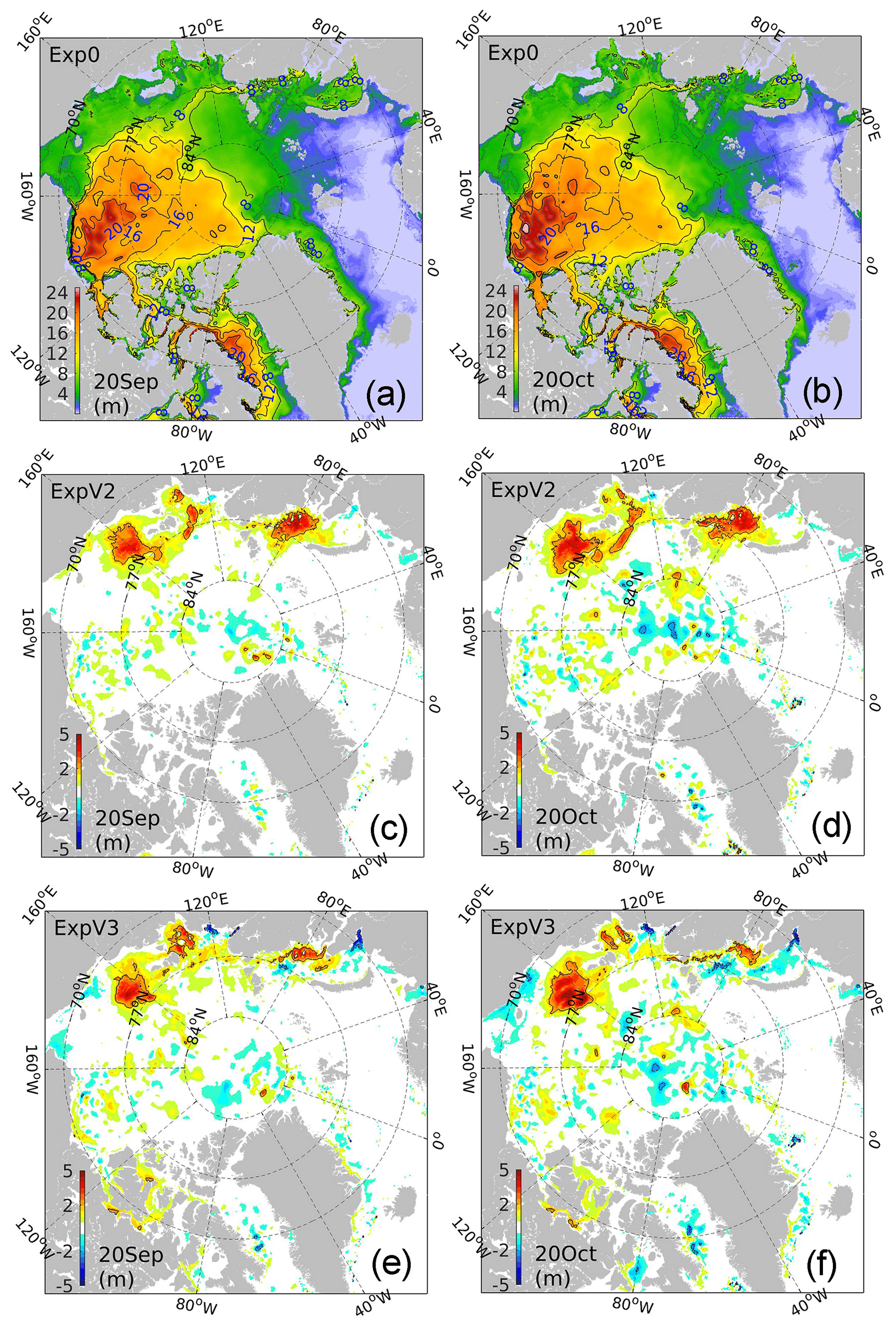
Figure 10 (a, b) Freshwater contents (unit: m) on 20 September and 20 October 2016 in the Arctic Ocean from the three assimilation runs: Exp0. The interval of isolines is 4 m. (c–f) The FWC differences in ExpV2 (c, d) and ExpV3 (e, f) concerning those in Exp0. The black lines indicate −2 and 2 m differences.

where the reference salinity value S_ref is taken at 34.8 psu, z_ref is the depth of the reference salinity or the sea bed, and S(z) is the salinity profile. Figure 10 shows the FWC on two representative days, 20 September and 20 October 2016. In Exp0, the reanalysis reproduces the typical FWC distribution in the Arctic, with a maximum in the Beaufort Sea.

The 20 m isolines in Fig. 10a and d show an increase in spatial coverage during October, consistent with Rosenblum et al. (2021), but the 20 m isoline does not extend as far as 170^∘ E compared to Proshutinsky et al. (2020). After the assimilation of SSS products (either V2.0 or V3.1), the amplitude and the spatial distribution of the FWC maximum increase slightly in the Beaufort Sea (see Fig. 10b and c). A much larger increase of FWC appears on the East Siberian shelf and in the coastal areas of the Laptev Sea and eastern Kara Sea, although to a different extent in ExpV2 and in ExpV3. In the eastern Kara Sea, the FWC increases over a wider area in ExpV2 than in ExpV3. To the west of the Yamal Peninsula, ExpV3 shows a negative anomaly related to an incorrect location of the model river runoff, corrected in later versions of the model. The SSS assimilation is able to correct the related fresh bias. In the central Arctic, although the assimilated SSS measurements are masked by the sea ice cover, the FWC differences north of 84^∘ N are more pronounced in October than in September, which indicates the advection of SSS increments by the Transpolar Drift Stream (Rigor et al., 2002; Balibrea-Iniesta et al., 2018). These results suggest that the SSS assimilation of both versions of SMOS satellite-based acts compensates for the insufficient river summer runoff, redistributes the freshwater in the Arctic, and adjusts the freshwater budget. However, because of the limited in situ data, the above assessment remains preliminary.

Further, we compare the daily time series of Arctic-averaged FWC from the three runs to the north of 70^∘ N (Fig. 11). The FWC increases in October–November to reach its maximum and gradually decreases thereafter. The impact of the week-long data assimilation cycles is visible as instantaneous jumps on the three curves of the time series, but the assimilation of SSS does not cause unrealistic imbalances. The FWC increases substantially by about 25 cm due to SSS assimilation. Notably, the assimilation of version 3.1 SSS causes a faster increase during the first 2 months. Due to the absence of ground truth data in 2016, the above comparison is not fully verified, but the timing of the peak is in better agreement with the seasonal freshwater storage presented by the Ice-Tethered Profiler (ITP) data in Fig. 4a of Rosenblum et al. (2021). In addition, we also notice that the amplitude of the seasonal FWC seems too small in all experiments in Fig. 11, which can be related to insufficient thick ice in TOPAZ (Uotila et al., 2019). More concrete evidence about the changed FWC will be provided when the longer assimilation of the satellite-based SSS product is finished in the near future.

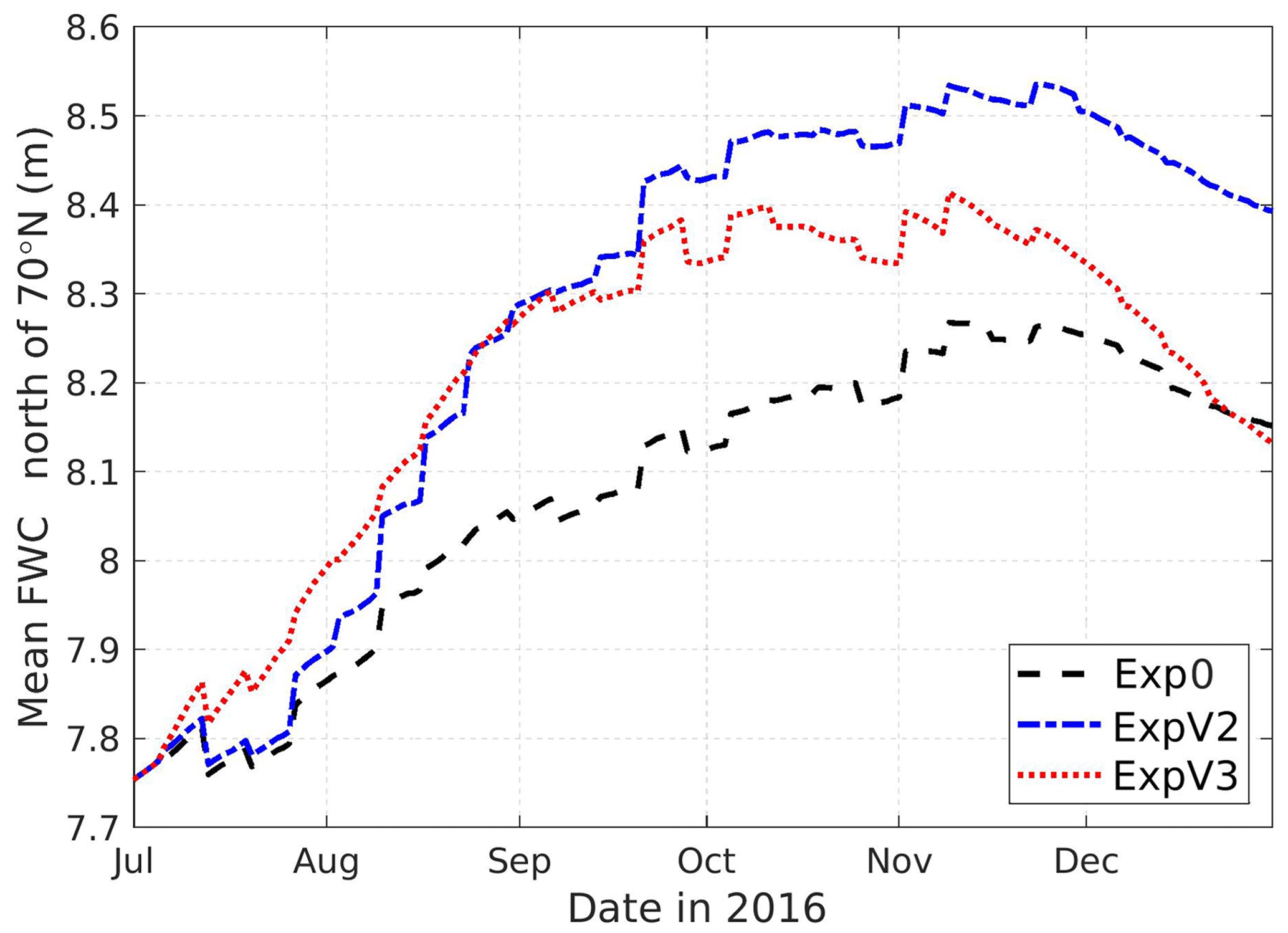
Figure 11 Arctic-wide averaged freshwater content (unit: m) in the central Arctic (> 70^∘ N) from July to December 2016 for Exp0 (dashed dark), ExpV2 (dashed blue), and ExpV3 (dotted red).

5 Summary and discussions

The gridded SSS products from the SMOS satellite undoubtedly provide a way to constrain errors in salinity, especially for an ocean reanalysis system. The present study is the first observing-system simulation experiment for the assimilation of SMOS SSS in the Arctic. In this study, based on the TOPAZ reanalysis system, we compared a reanalysis assimilating conventional observations with two new reanalysis runs which additionally assimilated two versions of the SMOS SSS products from BEC.

After comparison with independent SSS observations from CTD and surface water samples along cruise tracks, near-surface salinity errors have been significantly reduced compared to the control experiment (Exp0). In the Beaufort Sea, the SSS bias and RMSD in ExpV3 are reduced, respectively by 26.0 % and 20.6 %. In ExpV2, the RMSD reduction is smaller (by 11.5 %). In the Chukchi Sea, the reduction in SSS misfits in ExpV3 (bias:17.7 %; RMSD: 16.4 %) is also larger than in ExpV2 (bias: 15.5 %; RMSD: 13.7 %). Around Greenland, the difference between the two products is even more pronounced, with a significant reduction in the SSS bias (32.6 %) and RMSD (9.4 %) in ExpV3, while there is no notable improvement in ExpV2. The difference is larger in the east Greenland Sea. The direct assimilation of SSS from SMOS is more efficient at constraining the near-surface salinity than the multivariate impact of other observations. This finding is also consistent with other SSS assimilation experiments in the tropics (Chakraborty et al., 2015; Tranchant et al., 2019). Conversely, when considering the multivariate impact of SSS on SIC (in Fig. 9), we find that the assimilation of the V2 product does not affect the assimilation of sea ice concentrations, while the V3.1 product causes an increase in the negative increments, which could be an indication of excessive freshening along the Siberian coast. In contrast, the increments of SST in the open ocean are smaller in ExpV3, indicating a synergy effect of SST and SSS. Overall, our data assimilation system did not detect obvious inconsistencies between the SMOS SSS product and other assimilated observations.

Furthermore, this study shows error reductions of SSS when assimilating the V3.1 product from SMOS, even outside of the central Arctic in the Nordic Seas and along the Norwegian coast. Moreover, our analysis shows how the spatial distribution of Arctic FWC changes as a result of assimilating the two SMOS products. The time series of averaged FWC north of 70^∘ N shows that the FWC in the whole central Arctic can be increased by about 25 cm using DA. Our experiments show that the Arctic FWC can be redistributed horizontally after assimilation, but the latter effect requires a longer assimilation run to be evaluated.

As a summary of the quantitative SSS comparisons (Table 2), the overall score of each assimilation setup for each subregion can be defined by its ability to reduce the SSS bias and RMSD by more than 9 % relative to Exp0 (Fig. 2). The threshold value of 9 % is not fully arbitrary, referring to the reduction of SSS RMSD in GS, where the bias reduction is significant (through the t test). If both bias and RMSD meet this objective, we give a score of 1, but we give a score of 2 if only one of them is met. If neither of them exceeds 9 %, the score is set to 3. Thus, outside of the central Arctic, the v2.0 SSS product loses its impact on the TOPAZ system, but the V3.1 SSS brings about significant impacts across the Arctic and further out and clearly benefits from its refined effective resolution (Martínez et al., 2022). Since there was little evidence of a double-penalty effect in the validation RMSD apart from at Baffin Bay, we consider the assimilation of the higher-resolution signals to be efficient. However, the assimilation did not improve the SSS significantly in the Barents Sea or in other areas where SSS gradients are weak. These may require a higher accuracy to distinguish the Atlantic waters from other water masses of salinity only slightly below 35 psu. To further improve the SSS product, a combination with the Aquarius sensor using the same L-band frequency (e.g., Lee et al., 2012) and SMAP (e.g., Tang et al., 2017; Reul et al., 2020) is desirable.