Revisiting the tropical Atlantic western boundary circulation from a 25-year time series of satellite altimetry data

Geostrophic currents derived from altimetry are used to investigate the surface circulation in the western tropical Atlantic over the 1993–2017 period. Using six horizontal sections defined to capture the current branches of the study area, we investigate their respective variations at both seasonal and interannual timescales, as well as the spatial distribution of these variations, in order to highlight the characteristics of the currents on their route. Our results show that the central branch of the South Equatorial Current and its northern branch near the Brazilian coast, the North Brazil Current component located south of the Equator, and the Guyana Current have similar annual cycles, with maxima (minima) during late boreal winter (boreal fall) when the Intertropical Convergence Zone is at its southernmost (northernmost) location. In contrast, the seasonal cycles of the North Brazil Current branch located between the Equator and 7–8^∘ N, its retroflected branch, the northern branch of the South Equatorial Current to the west of 35^∘ W, and the North Equatorial Countercurrent show maxima (minima) during late boreal summer (boreal spring), following the remote wind stress curl strength variation. West of 32^∘ W, an eastward current (the Equatorial Surface Current, ESC) is observed between 2–2^∘ N, identified as the equatorial extension of the retroflected branch of the North Brazil Current. It is part of a large cyclonic circulation observed between 0–6^∘ N and 35–45^∘ W during boreal spring. We also observed a secondary North Brazil Current retroflection flow during the second half of the year, which leads to the two-core structure of the North Equatorial Countercurrent and might be related to the wind stress curl seasonal changes. To the east, the North Equatorial Countercurrent weakens and its two-core structure is underdeveloped due to the weakening of the wind stress. At interannual scales, depending on the side of the Equator examined, the North Brazil Current exhibits two opposite scenarios related to the phases of the tropical Atlantic Meridional Mode. At 32^∘ W, the interannual variability of the North Equatorial Countercurrent and of the northern branch of the South Equatorial Current (in terms of both strength and/or latitudinal shift) are associated with the Atlantic Meridional Mode, whereas the variability of the Equatorial Surface Current intensity is associated with both the Atlantic Meridional Mode and Atlantic Zonal Mode phases.

1 Introduction

The energetic western tropical Atlantic (WTA) boundary surface circulation is known to play a key role in the transport of heat, salt, and water mass from the Southern Hemisphere to the Northern Hemisphere of the Atlantic Ocean. It corresponds to a superposition of the return branch of the thermohaline Atlantic meridional overturning circulation (AMOC), the flow from the Atlantic Subtropical Cells, and Sverdrup dynamics (Schmitz and McCartney, 1993; Schott et al., 2004, 2005; Rodrigues et al., 2007; Tuchen et al., 2019, 2020). The region is also known to be influenced by large mesoscale activities due to the barotropic instabilities of the currents. The dominant mesoscale structures are the large rings generated by the North Brazilian Current (NBC) retroflection (Aguedjou et al., 2019; Aroucha et al., 2020). A regional scheme of the surface currents in the study area is proposed in Fig. 1. It is derived from a global analysis of the different studies mentioned hereafter.

From 5^∘ S to 15^∘ N, the surface boundary circulation is formed by the NBC flowing northward along the South American continental shelf. It carries tropical waters originating from the South Atlantic subtropical gyre and contributes to interhemispheric water transport (Johns et al., 1990, 1998; Peterson and Stramma, 1991; Stramma and England, 1999; Fratantoni et al., 2000; Silva et al., 2009; Zheng and Giese, 2009; Garzoli and Matano, 2011). The NBC has its origin near 5^∘ S, with the following two sources: the central branch of the westward South Equatorial Current (cSEC) and the along-shelf equatorward North Brazil Undercurrent (NBUC), which surfaces around 5–6^∘ S (Schott et al., 1998; Dossa et al., 2020). The latter advects warm waters from the South Equatorial Current (SEC) through its southern branch (Schott et al., 1995; Luko et al., 2021). Further north, around 5^∘ N, the NBC is also fed by the northern branch of the SEC (nSEC) (Goes et al., 2005). Following this, between 5–9^∘ N and 45–50^∘ W, a large part of the NBC retroflects to form a southeastward retroflected branch (hereinafter called rNBC). Between 3–8^∘ N, this branch first feeds the eastward North Equatorial Countercurrent (NECC) throughout the year, except during the boreal spring. At that time, the NECC is fed only by the North Equatorial Current (NEC) (Bourlès et al., 1999a; Goes et al., 2005). The NECC flows eastward between 2–12^∘ N and crosses the tropical Atlantic (Didden and Schott, 1992; Ffield, 2005; Urbano et al., 2008; Araujo et al., 2017). During the second half of the year, this current shows two cores that can separate into a southern and a northern branch (called sNECC and nNECC, respectively; Urbano et al., 2006; 2008).

At depth, around 3–8^∘ N, Cochrane et al. (1979) and Schott et al. (2004) suggested that part of the rNBC also feeds the eastward North Equatorial Undercurrent (NEUC) located around 5^∘ N. In addition, between 2^∘ S and 3^∘ N, the rNBC feeds the subsurface eastward Equatorial Undercurrent (EUC) (Hisard and Hénin, 1987; Bourlès et al., 1999b; Hazeleger et al., 2003; Hazeleger et de Vries, 2003; Schott et al., 1995, 2004). North of 10^∘ N, the part of the NBC that has not retroflected flows northwestward along the Guyana coast, forming the Guyana Current. The latter is also fed seasonally by the NEC (Johns et al., 1998) and transports warm equatorial waters into the Caribbean Sea (Stramma and Schott, 1999; Garzoli et al., 2003).

The WTA boundary surface circulation is driven by wind. In the vorticity equation, the terms that dominate locally are the Ekman pumping and the divergence of the geostrophic currents (Garzoli and Katz, 1983; Urbano et al., 2006). North of the Equator, the region is characterized by the strong seasonal variability of the wind. The trade wind variations influence the current system formed by the NBC, the NBC retroflection (NBCR), the rNBC, and the NECC. Specifically, the NBCR location, the NBC transport, and the NECC position and transport respond to the seasonal changes in the wind regimes (Johns et al., 1990, 1998; Garzoli et al., 2003, 2004; Urbano et al., 2006, 2008). This wind influence, which is related to the seasonal migration of the Intertropical Convergence Zone (ITCZ), is reflected in the latitudinal shifts of the currents. The variability in the current strength appears to be a regional response to the wind stress curl (WSC) distribution and strength over the basin (Johns et al., 1998; Fonseca et al., 2004; Garzoli et al., 2004, Urbano et al., 2006, 2008). In the equatorial region, the EUC seasonal variability depends on the basin-scale zonal pressure gradient and also on the seasonal cycle of the local wind forcing (Hisard and Hénin, 1987; Provost et al., 2004; Brandt et al., 2006, 2016; Hormann and Brandt, 2007).

The interannual variability of the WTA boundary currents has been understudied because of the lack of long-term data in this area. Nevertheless, Fonseca et al. (2004), using a combination of altimetry and hydrographic data from 1993 to 2000, investigated the influence of the wind on both the NBCR and the NECC variability. They did not find any direct relationship between them. Hormann et al. (2012) used the surface velocity data derived from drifters between 1993 and 2009 and highlighted a relationship between the NECC intensity and location and the tropical Atlantic climate modes (ACMs), represented by positive and negative phases of the Atlantic Zonal Mode (AZM) and Atlantic Meridional Mode (AMM) (Cabos et al., 2019). They found the intensity to be related to the cold phase of the AZM and the core location to be related to the warm phase of the AMM. In the equatorial Atlantic, Hormann and Brandt (2007) also found such a relationship using a high-resolution ocean general circulation model, observations, and sea surface temperature (SST) data. They showed that the EUC transport is affected by the cold and warm events of the AZM (the so-called “Atlantic Niño/Niña”) and confirmed the previous findings of Goes and Wainer (2003) concerning the link between the interannual variability of the wind and the AZM impacting the strength of the tropical Atlantic circulation.

In this study, we propose revisiting the scheme of the WTA boundary surface circulation using a 25-year time series of gridded altimeter-derived geostrophic currents. This dataset is longer than the one used by Fonseca et al. (2004) and allows us to provide a more robust description of the current branches described above and their seasonal and interannual variations. We also intend to analyze the regional relationship among these currents. The paper is organized as follows: in Sect. 2, the data and methods are presented. Section 3 brings some general characteristics of the current variability in the study area. In Sect. 4, we analyze and discuss the seasonal and spatial variabilities of the surface geostrophic currents and propose an updated seasonal map of the WTA surface circulation. The interannual variability of the circulation is analyzed in Sect. 5. Section 6 is devoted to a general discussion, and Sect. 7 offers a summary and some perspectives.

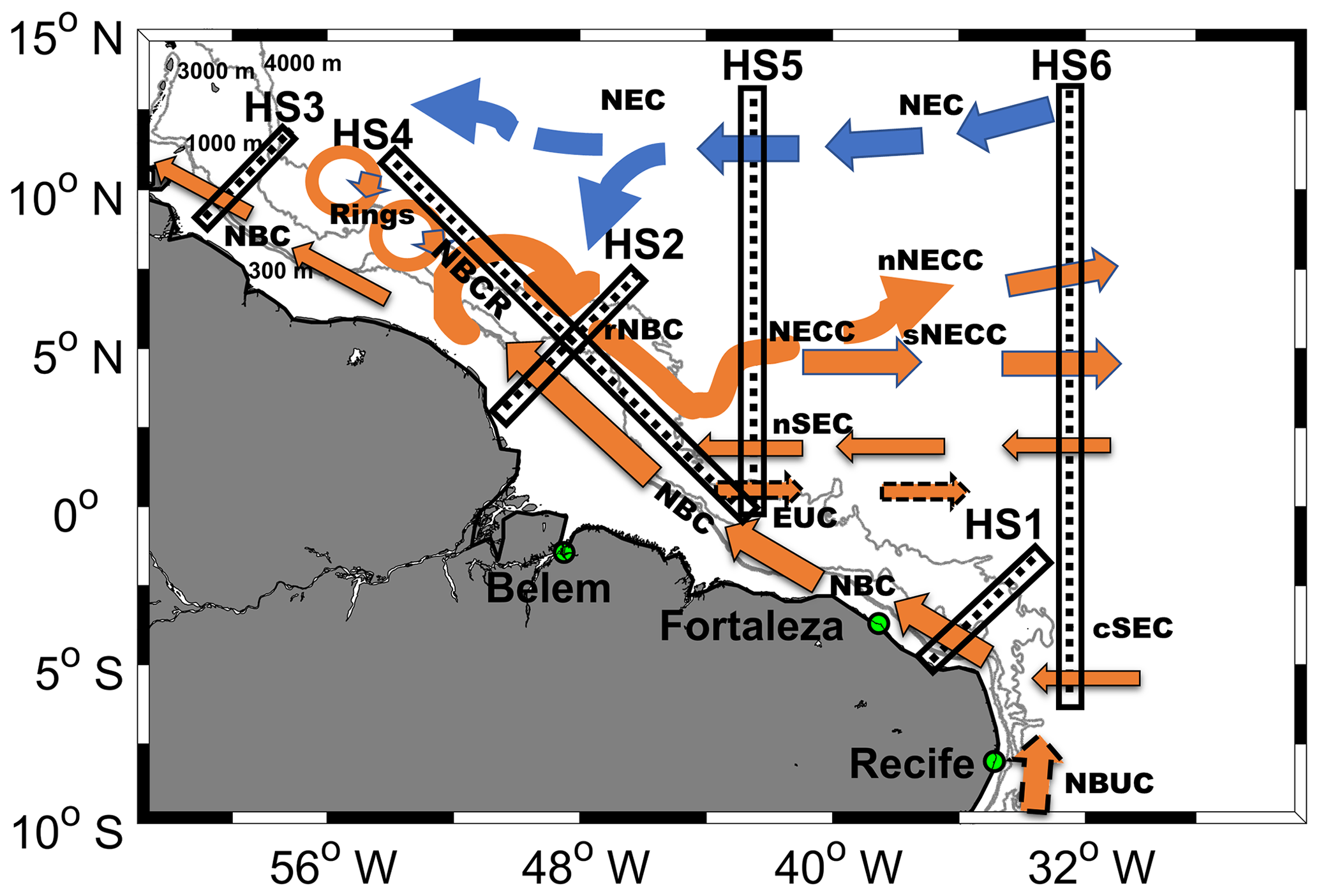
Figure 1 Schematic view of the western boundary surface circulation in the tropical Atlantic based on Schott et al. (2004), Goës et al. (2005), Urbano et al. (2006, 2008), and Aroucha et al. (2019). The distribution of the horizontal sections used to study the different current branches are also indicated in black: HS1, HS2, HS3, HS4, HS5, and HS6. Solid and dashed arrows are the upper and the subsurface currents, respectively. The blue and orange colors of the arrows show connections with the Northern Hemisphere and Southern Hemisphere waters, respectively. Acronyms are listed in Table A1 in the Appendix. The 300, 1000, 3000, and 4000 m isobaths (grey lines) are from the ETOPO2v1 database.

2 Data and methods

2.1 Altimeter-derived geostrophic currents

The Copernicus Marine Environment Monitoring Service (CMEMS) produces daily maps of ocean dynamic topography and derives geostrophic surface currents from along-track altimetry sea surface height measurements of all available satellite missions. Here, we use the SEALEVEL_GLO_PHY_L4_REP_OBSERVATIONS_008 _047 product (https://resources.marine.copernicus.eu, last access: 18 February 2023) from January 1993 to December 2017. The dynamic topography is estimated by optimal interpolation on a $\mathrm{0.25}{}^{\circ }\times \mathrm{0.25}{}^{\circ }$ global grid (details can be found in Pujol et al., 2016), and the geostrophic currents are computed using the nine-point stencil width methodology (Arbic et al., 2012) for latitudes outside the equatorial band (Equator ± 5^∘). In the equatorial band, the currents have been calculated using the Lagerloef methodology (Lagerloef et al., 1999), which used the β-plane approximation because the Coriolis parameter vanishes close to or at the Equator.

For the present work, focusing on the seasonal and interannual variability, the daily gridded velocity fields from CMEMS have been averaged monthly. Note that data with high variability (standard deviation >0.4) have been removed. They are found in the Amazon region, which is not a primary area of interest for this study, and where the annual mean current speeds are unrealistic (higher than 2.5 m s⁻¹), probably due to geographically correlated errors (Pujol et al., 2016). We have then defined six horizontal sections (called HS1, HS2, HS3, HS4, HS5, and HS6, respectively) that they cross at least one of the regional current branches perpendicularly (see Fig. 1). For each horizontal section, the original zonal and meridional surface velocity components have been rotated in order to derive the along-section and cross-section velocity components. In this study, we considered only the cross-section component, and the rotation angle considered for the oblique horizontal sections HS1, HS2, and HS3 is 45^∘ (HS4 uses 315^∘).

To validate geostrophic current estimates in the equatorial region, we have compared them to the PIRATA current meter mooring data available in the study area (0^∘ N, 35^∘ W) over the time period 11 October 2017–29 January 2018 (Fig. S1 in the Supplement). The data of the current meter were obtained at 12 m depth and have been averaged every 5 d. The results of the comparison with the geostrophic currents interpolated to the same location were in agreement with the results of the previous studies in the equatorial Pacific (Picaut et al., 1989; Lagerloef et al., 1999). However, in all these studies the geostrophic currents are underestimated compared to the direct velocity observations, and this is because the contribution of the ageostrophic velocities has not been considered (e.g., Fig. S1). The correlation of 0.71 is found on their zonal components, while the one on the meridional components is lower (<0.5) (Fig. S1a–b). The mean biases (differences) in standard deviation for both components are, respectively, 0.04 (0.11) m s⁻¹ and 0.14 (0.03) m s⁻¹. Similar values were also found by Lagerloef et al. (1999) in the western equatorial Pacific when comparing the geostrophic currents to the current meter mooring data at 10 m depth. These results give credit to the geostrophic estimates used in this work for the equatorial region even though their values are underestimated compared to other observations (Picaut et al., 1989; Lagerloef et al., 1999; Pujol et al., 2016).

2.2 Wind velocity

Monthly wind velocity fields from the ERA5 atmospheric reanalysis produced by the European Centre for Medium-Range Weather Forecasts (ECMWF, http://www.ecmwf.int, last access: 18 February 2023) are used in order to evaluate the influence of the remote winds on the WTA ocean circulation. They were downloaded from the Copernicus Climate Change data server over the January 1993–December 2017 period. We used the wind velocity data to calculate the wind stress field as follows.

The zonal and meridional components of the wind stress, τ_x and τ_y, are calculated using empirical formulations (Large and Pond; 1981: Gill, 1982; Trenberth et al., 1990) following NRSC (2013):

$$\begin{array}{}\text{(1)}& {\displaystyle }{\mathit{\tau }}_x={\mathit{\rho }}_{\text{air}}{C}_{\text{D}}W\cdot U,\text{(2)}& {\displaystyle }{\mathit{\tau }}_y={\mathit{\rho }}_{\text{air}}{C}_{\text{D}}W\cdot V,\end{array}$$

where U and V represent the zonal and meridional wind velocity components, respectively, W represents the wind speed amplitude, ρair represents the air density (1.2 kg m⁻²), and C_D represents the drag coefficient at the ocean surface calculated according to Large and Pond (1981).

The wind stress curl (WSC) is then deduced following Gill (1982):

$$\begin{array}{}\text{(3)}& \text{Curl}\left(\mathit{\tau }\right)={\displaystyle \frac{\partial {\mathit{\tau }}_y}{\partial x}}-{\displaystyle \frac{\partial {\mathit{\tau }}_x}{\partial y}}.\end{array}$$

Over the tropical Atlantic, the ITCZ location has been determined from the WSC near-zero values. In addition to this, the minimum and maximum of the negative and positive WSC values have been derived, while the WSC strength values (sum of the absolute minimum negative and maximum positive values) have also been computed. Each of these parameters is zonally averaged over the region covering 6^∘ S–16^∘ N and 30^∘ W–0^∘ E, following Fonseca et al. (2004).

2.3 Sea surface temperature

Monthly estimates of sea surface temperature (SST) are also used in order to compute the Atlantic climate mode indexes and evaluate their possible relationship with the interannual changes observed in the WTA boundary circulation. A global gridded SST product with a 1^∘ spatial resolution is downloaded from the NOAA repository (https://www.esrl.noaa.gov/psd/data/gridded/data.noaa.oisst.v2.html, last access: 19 February 2023, Reynolds et al., 2002). The AZM index is calculated considering the SST anomalies (SSTAs) relative to the 1993–2017 monthly climatology in the ATL3 region bounded by 3^∘ S–3^∘ N and 20^∘ W–0^∘ E (Zebiak, 1993; Hormann et al., 2012). The AMM index is also based on SSTAs relative to the 1993–2017 monthly climatology and calculated as the difference between the spatial average SSTA in the box 5^∘ N–25^∘ N and 60^∘ W–20^∘ W and the spatial average SSTA in the box 20^∘ S–5^∘ N and 30^∘ W–10^∘ E (Servain, 1991; Hormann et al., 2012).

3 General characteristics of the circulation in the western tropical Atlantic

The mean WTA surface geostrophic circulation is first derived by averaging the gridded altimetry current maps over 1993–2017 (Fig. 2a). We distinguish the following three different areas (from the southeast to the northwest).

1. The NBC formation area starting around 5^∘ S includes the westward cSEC flowing north of 6^∘ S (mean value of ∼0.3 m s⁻¹) that feeds the NBC–NBUC current system around 34–36^∘ W. The NBC amplitude increases along its northward along-shelf course, up to 0.8 m s⁻¹ around 3^∘ S. It then slows down toward the Equator, before increasing again north of 3^∘ N. Farther north along the coast, its mean velocities are again weaker, with values of ∼0.3 m s⁻¹.

2. The NBC retroflection region between 5–8^∘ N shows includes where the NBC undergoes an eastward recirculation, which feeds a southeastward current, i.e., the so-called the NBC retroflected branch (rNBC). The rNBC reaches annual mean velocities of ∼0.6 m s⁻¹.

3. The area between 3–6^∘ N and 42–46^∘ W includes the area where rNBC meanders with an annual mean velocity of 0.5 m s⁻¹ and partly feeds the surface eastward NECC, which decays along its course. This area is located in a region of high wind variability (not shown in this paper).

In addition, we also observe the westward nSEC flowing between 2–6^∘ N, with stronger velocity values in the eastern part of the basin (mean velocity larger than 0.3 m s⁻¹).

We computed the mean power spectral density of the daily geostrophic current time series in order to detect the dominant components of the WTA current variations (not shown). It highlighted the following three main energy zones:

1. at intraseasonal timescales, with different peaks for periods of fewer than 120 d,

2. at seasonal timescales,

3. at interannual timescales, with peaks for periods larger than 600 d.

We then filtered the velocity time series using different cutoff frequencies in order to isolate each of this component of the current variability: below 120 d, between 120 and 600 d, and above 600 d. We computed the ratio between the standard deviation of each filtered current field and the total current field. The resulting maps (Fig. 2b–d) show the relative importance of each component with regard to the total variance as a function of the location. We observe the predominance of the seasonal variability in the whole WTA (overall ratio of 0.44), with the highest values (0.48) observed along the continental shelf, in the NBC region, and between 0–2^∘ S east of 36^∘ W. Intraseasonal fluctuations are also important in the same areas (with the largest ratio of 0.44), while the interannual variability is weaker, with the highest values (>0.2) observed in the NECC area north and east of 4^∘ N and 40^∘ W, respectively (consistent with Richardson and Walsh, 1986). In this study, we focus on the seasonal and interannual timescales.

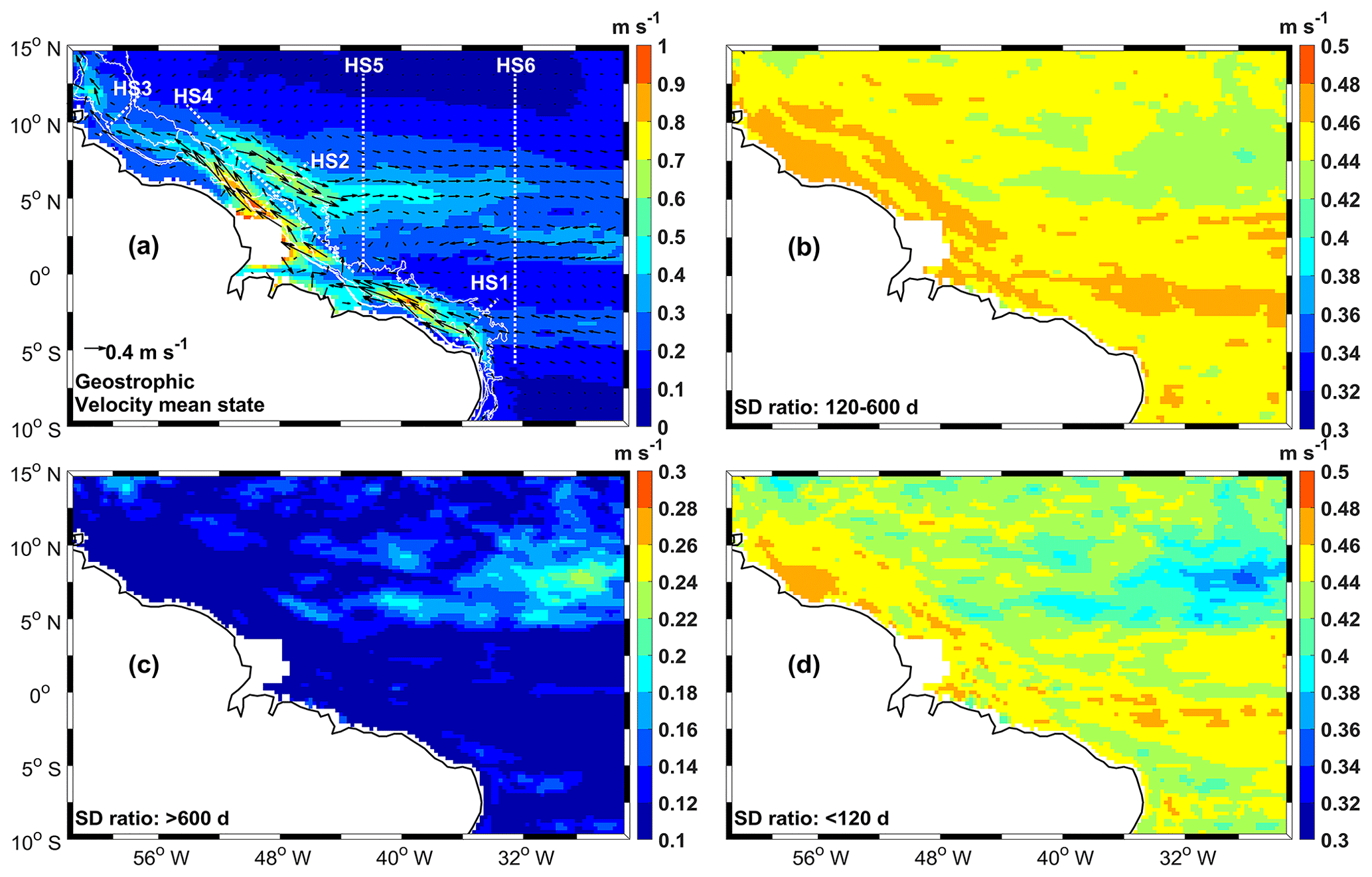
Figure 2 (a) Temporal mean of the geostrophic currents (amplitude in m s⁻¹ and vectors) in the study area between 1993 to 2017. Panels (b), (c), and (d) show the ratios between the standard deviations of the currents for the signals between 120 and 600 d, longer than 600 d and shorter than 120 d, respectively, and the standard deviation of the total currents. The dashed white lines labeled HS1, HS2, HS3, HS4, HS5, and HS6 in (a) represent the cross sections of the currents, and the solid white lines are the 300, 1000, 3000, and 4000 m isobaths. Note that the color bar in (c) is different from the ones in (b) and (d).

To further investigate the variability of the different current branches, we then averaged the daily geostrophic currents on a monthly basis and extracted the cross-sectional geostrophic velocities along the six horizontal sections defined above (Fig. 1). In order to remove the intraseasonal variability, the monthly velocity estimates are further refined using a low-pass filter with a 4-month cutoff frequency. The time–space diagrams (also called Hovmöller diagrams) along the six horizontal sections are plotted in Fig. 3. We can clearly observe large changes in both time and space with respect to the different current branches, illustrating the complexity of the surface circulation in the WTA. The seasonal and, to a lesser extent, interannual current fluctuations mentioned above are clearly visible in the different horizontal sections. For each of the horizontal sections, the time-averaged current values are also computed as a function of the latitude (plots on the left side of each panel in Fig. 3), highlighting the mean spatial extension of the current paths crossing the corresponding horizontal section. Note that in addition to the main currents mentioned in Fig. 1, between 2^∘ S–2^∘ N HS4 to HS6 show an eastward surface current at the same location as the subsurface EUC, i.e., west of 44^∘ W along the Equator (Schott et al., 1998). Depending on the season, the EUC core is known to be located at a depth between about 50–100 m (Brandt et al., 2016). At 44^∘ W, Bourlès et al. (1999b) have also noticed the presence of an eastward surface flow above the EUC, which was identified to be different than the EUC. The presence of this eastward surface flow is also confirmed by the PIRATA current meter data available in our study area (0–35^∘ W, from November 2018 to March 2019; see Fig. S1). These findings motivate our investigation of the variability of the surface currents in the equatorial part of our study area. We chose to name this eastward surface flow the Equatorial Surface Current (ESC) in order to further investigate this signal, which is also captured on HS4, HS5, and HS6.

Table 2 summarizes the mean current width derived along the different horizontal sections (using the plots on the left side of each panel in Fig. 3). Note first that a positive current convention is chosen for the horizontal sections as follows: northward NBC along HS1 to HS3, eastward NBCR along HS4, eastward NECC along HS5 and HS6, and eastward ESC along HS4 to HS6. Hence, the signatures of the rNBC (HS2), the nSEC (HS4 to HS6), and the cSEC (HS6) are considered negative. From Table 2, we observe that the NBC becomes narrower from HS1 to HS2. The retroflection zone (HS4, Fig. 3) extends from 3.7 to 10.5^∘ N, in agreement with Fonseca et al. (2004), who found the northernmost position of the NBCR around 11^∘ N. North of the retroflection, the NBC along the Guyana coast is weaker but broader relative to HS2 (NBC2 and NBC3 in Fig. 3). The nSEC signature changes from HS6 to HS4. It is wider at 32^∘ W (nSEC6), narrower at 42^∘ W (nSEC5), and wider again closer to the shelf at 44^∘ W (nSEC4) ( 550, 67, and 190 km in Table 2, respectively). The NECC extension also varies from 32 to 42^∘ W and is wider and located further north toward the east, with a mean width extending from 860 km (NECC5) to 920 km (NECC6).

Table 1 Extension in latitude and kilometers for the different current branches crossing the different horizontal sections: NBC1, NBC2, and NBC3 are the North Brazil Current captured along HS1, HS2, and HS3, respectively; NECC5 and NECC6 are the North Equatorial Countercurrent captured along HS5 and HS6, respectively; nSEC4, nSEC5, and nSEC6 are the northern branch of the South Equatorial Current (SEC) captured along HS4, HS5 and HS6, respectively; cSEC6 is the central branch of the SEC captured along HS6; and ESC4, ESC5, and ESC6 are the Eastward Equatorial Surface Current captured along HS4, HS5, and HS6, respectively.

Figure 3 Hovmöller diagrams (1993 to 2017) of the cross-sectional current components (m s⁻¹) for HS1, HS2, HS3, HS4, HS5, and HS6. The time average over the section is shown (thick lines), framed by the corresponding standard deviation (thin lines), on the left side of each panel. The color shading shows the northward and eastward (red) or southward and westward (blue) direction of the cross-current. Acronyms are listed in Table A1. The numbers next to the acronyms represent the number of the horizontal section. The green line in the HS1 plot indicates the time series of the maximum velocity of the cross-sectional current (NBC) and is framed by the time series of the maximum velocities divided by 2 (blue lines) over 1993–2017 period.

In order to further investigate the temporal variations of the current strength, the maximum speed values of each current path have been determined for each month. The maximum speed corresponds to the current core velocity and is hereafter called V_max (see Fig. 3, green line in the HS1 plot). The location of the core velocity is also computed. In addition, to estimate the current relative strength and intensity, we have considered the part of the horizontal sections of velocities larger than $V_{\text{max}}/$2 (see Fig. 3, blue lines in the HS1 plot), and we finally computed the values by averaging the velocity values over the area where $V_{\text{max}}/\mathrm{2}<V<V_{\text{max}}/\mathrm{2}$. The width of the currents (Table 2) is determined by the average velocity values over the whole period of study (1993–2017) (see left boxes of the Hovmöller diagrams of Fig. 3). In addition, knowing the sign or direction of the current (eastward or westward), the zero contours of the velocity fields are used to define the width of the currents. Note that the current strength and intensity have also been computed by averaging velocity values over the entire width of the current paths (e.g., not only where the velocity is larger than V_max/2), but the results did not correctly reflect the current variability observed in Figs. 3 and 4 (not shown).

For the NBCR and NECC, the variability of the maximum speed of the two apparent flows and branches and their corresponding locations is also analyzed in order to compare the results with the study of Fonseca et al. (2004). The goal is also to investigate the variability of the current location with respect to the wind variability and the tropical Atlantic climate modes. In this study, the presence of two flows of the NBCR and the NECC two-core structure are identified when the velocity profile shows two local maxima separated by a local minimum in the NBCR region (between 4—10^∘ N) and the NECC region (between 3–11^∘ N), respectively (Fig. 4, HS4–HS6).

4 Seasonal variability

Here we focus on the seasonal cycle of the different current branches observed in the study area. Therefore, a monthly climatology of the velocity estimates shown in Fig. 3 is calculated for each of the six horizontal sections (Fig. 4). For further analysis, the monthly climatology of V_max, V_max location, and relative current intensity have also been derived from the corresponding monthly time series for different current components (Fig. 5).

4.1 The North Brazil Current and its retroflection

In Fig. 4, the NBC (HS1) and the cSEC (HS6) are both observed located at ∼4^∘ S and present similar seasonal cycles, with stronger flows during the first half of the year. The cSEC6 velocity maximum (0.3 m s⁻¹) and minimum (0.1 m s⁻¹) appear in May and October, respectively. The NBC1 velocity maximum (0.6 m s⁻¹) and minimum (0.4 m s⁻¹) appear in May–June and November–December (Fig. 5a), respectively. These annual cycles are also similar to the annual cycle of the NBUC transport observed by Rodrigues et al. (2007) at 10^∘ S, which is related to the bifurcation location of the sSEC at about 10–14^∘ S near the surface. This suggests that the seasonal variability of the NBC might, at its southernmost location, be partly driven by the location of the sSEC bifurcation, which has been shown to be influenced by the annual cycle of the WSC over the area 5–10^∘ S, 25–40^∘ W (Rodrigues et al., 2007).

When comparing the NBC along HS1, HS2, HS3, and HS4 (Figs. 4 and 5), it clearly depicts two different seasonal cycles along its northward path. The NBC2, NBCR4, and rNBC2 flows show approximately the same seasonal cycles and are in opposite phase with the NBC1 and NBC3 flows. NBC2 is more narrow but relatively strong when compared to NBC1. It decreases from January to May (by ∼0.4 m s⁻¹) and then increases again to reach a maximum in November–December (1 m s⁻¹). Compared to NBC2, rNBC2 is broader (width of ∼350 km against 20 km) but less intense (maximum of 0.6 m s⁻¹ in November–December). Apparently, the NBC2 width and strength seem to be linked to the nSEC intensity in the eastern basin (see nSEC6 and nSEC4 in Fig. 5b). When the nSEC is weaker, NBC2 is also weaker and narrower. In addition, NBC2 intensifies when nSEC intensity increases. This shows the importance of the nSEC contribution to the NBC in the Northern Hemisphere. The delay between the nSEC and NBC2 growth could be due to the mesoscale activities being more intense in the western basin (Aguedjou et al., 2019). The fact that the NBC1 and NBC3 flows are in phase when the nSEC contribution to NBC2 is lower might also indicate that the NBC is more stable when the intrusion of water from the nSEC is weak. The latter may generate barotropic and baroclinic instabilities of the NBC, which then tend to retroflect eastward. This could explain the phasing of the annual cycle of NBC2, NBC4, and rNBC2.

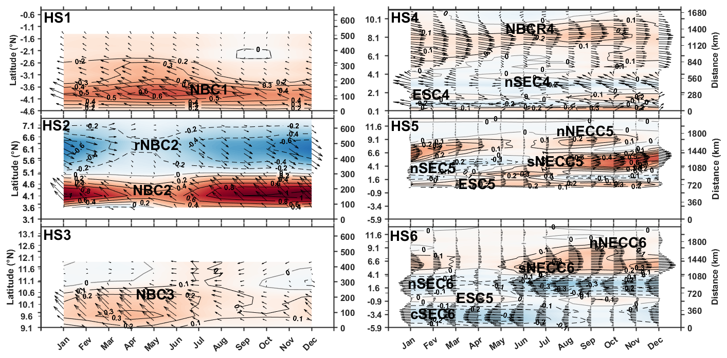
Figure 4 Average seasonal cycle obtained from Fig. 3 (vectors of the currents are superimposed on the contour of their amplitude in m s⁻¹). The distances from the southernmost point (in km) are indicated on the right-hand y axis of each panel.

In Fig. 4, from September to January we observe two retroflections of the NBC: the main one around 8^∘ N and a secondary one more to the south between 4–6^∘ N (Figs. 4 (HS4) and  5c). The flow of this secondary retroflection (called sNBCR) reaches its maximum intensity in October, while the main retroflection flow (called nNBCR) reaches its maximum 1 month earlier. Following this, it migrates northward to join the nNBCR4 and both flows are completely merged at the beginning of the following year (Fig. 4, HS4). Both branches merge at the beginning of the year, and the NBCR then weakens to reach its minimum intensity in May. Note that the seasonal cycles of NBC2 and the NBCR are similar to the one of the NBC transport obtained by Johns et al. (1998) and Garzoli et al. (2004) using acoustic Doppler current profilers (ADCPs), inverted echo sounders, and pressure gauge data. Johns et al. (1998) related the seasonal cycle of the NBC observed in this area to the remote wind stress curl forcing across the tropical Atlantic. Here, we also see that the seasonal cycles of the NBC branches north of the Equator (except the NBC continuity along the Guyana coast) seem to follow the remote wind stress curl strength with a delay of 1 to 4 months (Fig. 5a–f). The latter should be impacted by the mesoscale activities and/or wave propagations in the region (Fonseca et al., 2004). The northernmost location of the nNBCR maximum intensity occurs in August, when the maximum WSC strength is reached (Fig. 5c and f). The root mean square (rms) of the monthly mean values of its location (Fig. 5c) is nearly constant ($\sim \mathrm{2.3}{}^{\circ }$) and is consistent with the fact that there may not be a preferred season for NBC ring formation (Garzoli et al., 2003; Goni and Johns, 2003). Indeed, Garzoli et al. (2003) have shown using inverted echo sounder observations that there was a link between the rapid northward and southward extension of the NBC retroflection and the shedding of the rings in this region.

Farther north, the NBC component flowing along the Guyana coast (NBC3) is twice as wide (∼440 km) and less intense than NBC2 (Fig. 4, HS2–HS3). It reaches a minimum in October (∼0.1 m s⁻¹) and a maximum during March–May (0.3 m s⁻¹) when NBCR4 is at a minimum (Figs. 4 (HS3–HS4) and  5). As already mentioned, its seasonal cycle is similar to NBC1 and the cSEC and might also be influenced by the sSEC bifurcation location.

4.2 The North Equatorial Countercurrent

The NECC (both NECC5 and NECC6) seasonal cycle is similar to the ones of the NBC2, NBCR4 and rNBC2 (Fig. 4, HS2, HS4, HS5, and HS6). It weakens along its pathway and its intensity is at its maximum in November–December (∼0.6 m s⁻¹ at 42^∘ W and ∼0.3 m s⁻¹ at 32^∘ W) and minimum in April–May (Fig. 5a).

During the second part of the year, we observe the two-core structure previously investigated by Urbano et al. (2006, 2008). The two cores and branches are seen first at 42^∘ W in August and then at 32^∘ W in September (Figs. 4 and 5d–e). The northern branch (nNECC) is narrower (between 7–9^∘ N) and stronger (0.3 m s⁻¹) in August–September at 42^∘ W (Figs. 4 (HS5) and 5d). It is even separated from the southern branch from October to December. At 32^∘ W, the northern core and branch is stronger from September (northern core velocity of ∼0.2 m s⁻¹) to November. It gradually decreases in intensity and shifts northward until forming a separated second branch, located between 9–11^∘ N, from December to February and then becomes very weak in March–April (Figs. 4 (HS5) and 5e).

From June to July, the NECC signature (sNECC branch) is located between 3–4^∘ N at 42^∘ W and is connected from the south to the eastward flow associated with ESC5 in Fig. 4 (HS5). Urbano et al. (2008) showed with ADCP data at 38^∘ W that the eastward NECC cycle may start in this region when the EUC is shallower and further north and also seems to be connected to a shallower NEUC during this period of the year. The presence of the ESC5 suggests that it may be the one that favors the surfacing and the connection of both currents during June–July. From June to November, the sNECC branch increases simultaneously with rNBCR2. However, it reaches its maximum 1 month earlier (November) and starts decreasing when the rNBC is still increasing. This confirms that the NECC is not only fed by the rNBC at the surface as suggested by Verdy and Jochum (2005). The sNECC witnesses the same variability at both 32 and 42^∘ W but reaches its minimum early in March–April at 32^∘ W when the climatological NECC is described in the literature as a reversing flow or is missing at its usual location (Garzoli and Katz, 1983; Garzoli, 1992). At this location (32^∘ W), the sNECC starts increasing from April–May far from the ESC (between 4–6^∘ N) and grows until November. Burmeister et al. (2019) showed that when the ITCZ migrates northward (April to August) (Fig. 5f) in the central Atlantic, the nSEC recirculates eastward to reach the NEUC (which then increases). The presence of the sNECC flow in April–May may suggest that the NECC flow might be initiated by an eastward recirculation of the nSEC, which flows on top of the NEUC during this period. It reaches its first maximum in July–August together with the nSEC and a second maximum in November (Fig. 5a–b and e).

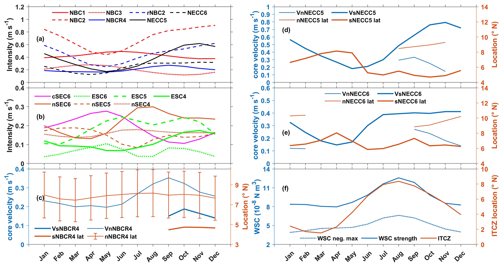
Figure 5 Monthly climatology of the relative current speed (m s⁻¹) (a–b); core velocities and locations in the NBCR regions (c); the core velocities and locations of the NECC branches along HS5 and HS6 (d–e); and the absolute values of the maximum negative wind stress curl (WSC neg. max), WSC strength, and ITCZ location (f). Acronyms are listed in Table 1, and the numbers next to the acronyms represent the numbers of the horizontal sections. In (c), (d), and (e), the core velocities and locations are shown in blue and orange, respectively.

At 32 and 42^∘ W the sNECC shows two northward migrations (Fig. 5d–e). The first one occurs from June–July (June) to August (September) at 42^∘ W (32^∘ W), and the second one occurs from October to April. Fonseca et al. (2004) also found such behaviors but with some differences, i.e., the two northernmost NECC locations in February and August and the two southernmost NECC locations in June and December. However, they lacked data between March and May, and we do not use the same methods to compute the core position.

4.3 The central and northern branches of the South Equatorial Current

The cSEC and nSEC, which are two branches of the westward SEC, do not have the same seasonal cycle (Fig. 4, HS4–HS6). This is due to the fact that the nSEC can be affected in the Northern Hemisphere by the southeast trade winds that cross the Equator. However, nSEC4, nSEC5, and nSEC6 have maxima at different periods of time. At 32^∘ W, nSEC6 increases from April onward to reach a maximum of ∼0.3 m s⁻¹ in August, following the migration of the ITCZ (Fig. 5b and f). During this time, at 42^∘ W nSEC5 migrates northward, while its intensity decreases until July, when it almost disappears. The ESC then appears (Fig. 4, HS5). The nSEC5 flow is observed again after July, and it increases and reaches a maximum of ∼0.2 m s⁻¹ in March (Figs. 4 (HS5–HS6) and 5b). Over the continental shelf, most of the nSEC joins the NBC (HS4, around 2–4^∘ N and 46^∘ W) and a part deviates southeastward to join the rNBC and form the eastward ESC4 flow (captured along HS4; see Fig. 4). The nSEC component that joins the NBC reaches its maximum of ∼0.2 m s⁻¹ between June and August (also following the ITCZ northward migration, Fig. 5b and f). However, the nSEC seasonal variations are relatively small (∼0.15 m s⁻¹) (Fig. 4, HS4). This is also true for nSEC4, but the angle of the horizontal section relative to the flow probably leads to a significant reduction in the current amplitude captured.

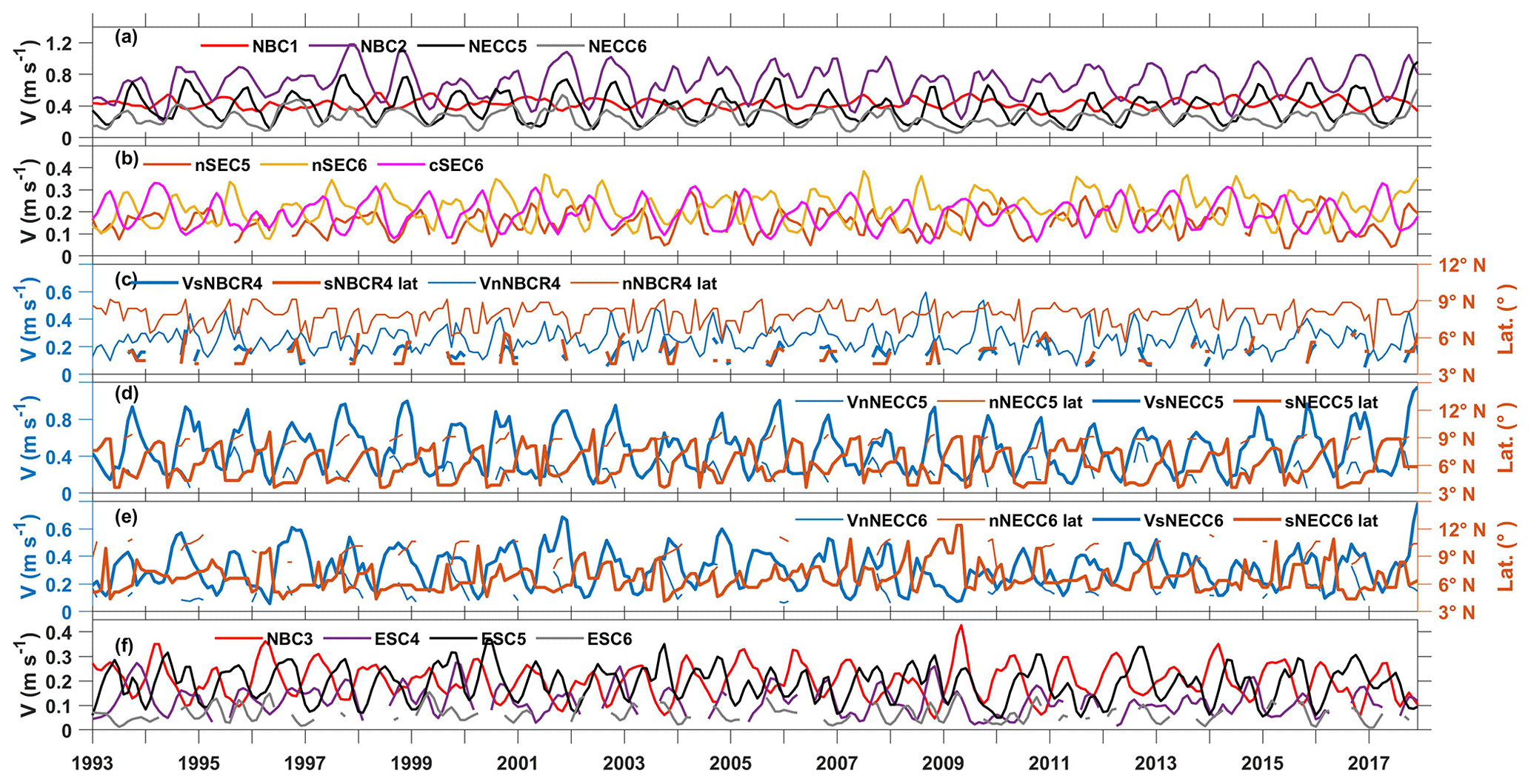
Figure 6 Time series of the 4-month low-pass-filtered characteristics of the geostrophic currents (a–f) captured along HS1 to HS6. Acronyms are listed in Table 1, and the numbers next to the acronyms represent the number of the horizontal sections. (a) Intensity of NBC1, NBC2, NECC5, and NECC6. (b) Intensity of cSEC6, nSEC5, and nSEC6. Panels (c), (d), and (e) show the core velocities and the locations of the nNBCR4 and the sNBCR4 flows; the nNECC5 and the sNECC5 flows; and the nNECC6 and the sNECC6 flows, respectively. (f) Intensity of the NBC3, ESC4, ESC5, and ESC6 flows.

4.4 The Equatorial Surface Current

Figure 4 (HS4–HS6) shows the presence of an eastward current near the Equator. Such a feature was already observed and mentioned by Hisard and Hénin (1987) and Bourles et al. (1999b) using hydrographic and ADCP data. In Fig. 4 (HS4), eastward flows are captured between 1–2^∘ N (ESC4) and along the Equator. As mentioned in Sect. 4.3, they may be composed of the part of the nSEC that does not join the NBC and the rNBC (which is known to feed the EUC in the thermocline layer). The weaker intensity of ESC4 compared to ESC5 (i.e., ESC at 42^∘ W) is explained by the angle between HS4 and the current direction. However, the weaker intensity of ESC6 (i.e., ESC at 32^∘ W) is due to the weakening of the corresponding eastward flow between both longitudes. ESC4 and ESC5 are observed almost throughout the year (Fig. 4, HS4–HS6), and their amplitude follows a semi-annual cycle (Fig. 5b) similar to the EUC in the eastern Atlantic (Hormann et al., 2007). However, the periods of the maxima are slightly different from one location to the other. The ESC4 semi-annual cycle shows a weak maximum in March–April (∼0.1 m s⁻¹) and another maximum in November (∼0.2 m s⁻¹). The ESC5 amplitude is larger because of the merging of ESC4 with the eastward flow observed along the Equator (Fig. 4, HS5). Its maxima occur in June and October with similar intensities (more than 0.2 m s⁻¹) (Fig. 5b). ESC6 (at 32^∘ W) is weaker but reaches its maxima in May and in September-October (less than 0.1 m s⁻¹). Since this eastward ESC current component is almost undocumented in the literature, we will discuss it further in Sect. 6. Note that (as mentioned in Sect. 2.1) the ESC amplitude captured in the altimetry product here is probably underestimated compared to the observations.

5 Interannual variability

Beyond the dominant seasonal variability of the circulation at regional scale, we also observe a year-to-year variability of the surface velocities in the study area (Figs. 2 and 3). The latter is analyzed here using the time series of the characteristics (intensity and core velocity and location; see Sect. 3) of the different current branches captured along the six horizontal sections (Fig. 6). We will also analyze this variability in light of the tropical Atlantic climate modes.

In Fig. 6a–b over the whole study period we observe that the intensities of cSEC6 (cSEC along HS6), NBC1 (NBC along HS1), and NBC2 (NBC along HS2) vary between 0.05–0.35 m s⁻¹, 0.3–0.6 m s⁻¹, and 0.2–1.2 m s⁻¹, respectively, with corresponding mean values of 0.2 m s${}^{-\mathrm{1}}\pm \mathrm{0.06}$, 0.4 m s${}^{-\mathrm{1}}\pm \mathrm{0.06}$, and 0.7 m s${}^{-\mathrm{1}}\pm \mathrm{0.2}$, respectively. To the north, when crossing HS3, the NBC weakens and ranges between 0.05–0.43 m s⁻¹, with a mean intensity of 0.2 m s${}^{-\mathrm{1}}\pm \mathrm{0.07}$. In the equatorial region (±5^∘ of latitude), along HS5 and HS6, the nSEC intensity varies between 0.05–0.3 m s⁻¹/0.1–0.4 m s⁻¹, with a mean value of 0.15 m s⁻¹ ± 0.05/0.2 m s⁻¹ ± 0.07 (Fig. 6b). The ESC intensity varies between 0.15–0.3, 0.05–0.4, and 0–0.15 m s⁻¹ when crossing HS4, HS5, and HS6, respectively, with corresponding mean values of 0.12 m s${}^{-\mathrm{1}}\pm \mathrm{0.05}$, 0.2 m s${}^{-\mathrm{1}}\pm \mathrm{0.07}$, and 0.06 m s${}^{-\mathrm{1}}\pm \mathrm{0.03}$.

The two-core structures of the NECC and NBCR regions show the highest year-to-year variations in both velocity and location (Fig. 6c–e). The NECC and NBCR intensity and core velocity were found to be significantly correlated (>0.98) (sNECC and nNBCR; figure not shown). At 42^∘ W, the sNECC and nNECC velocity cores vary between 0.1–1.2 m s⁻¹ and 0.05–0.55 m s⁻¹, respectively, with respective mean values of 0.5 m s${}^{-\mathrm{1}}\pm \mathrm{0.25}$ and 0.25 m s${}^{-\mathrm{1}}\pm \mathrm{0.1}$. They are located between 3.6–9.9^∘ N and 7.6–10.4^∘ N, respectively, with respective mean locations at 6.1^∘ N ± 1.7^∘ and 8.9^∘ N ± 0.8^∘ (Fig. 6d). At 32^∘ W, the cores vary between 0.05–0.8 m s⁻¹ and 0.05–0.5 m s⁻¹, respectively, with respective mean velocities of 0.3 m s${}^{-\mathrm{1}}\pm \mathrm{0.13}$ and 0.2 m s⁻¹ ± 0.09. They are located between 4.1–12.4^∘ N and 7.4–11.6^∘ N, respectively, with respective mean locations of 6.6^∘ N ± 1.4^∘ and 9.7^∘ N ± 1.1^∘ (Fig. 7e). The sNBCR and nNBCR maximum speeds crossing HS4 vary between 0.05–0.3 m s⁻¹ and 0.05–0.6 m s⁻¹, respectively, with respective mean values of ∼0.15 m s⁻¹ ± 0.06 and 0.25 m s${}^{-\mathrm{1}}\pm \mathrm{0.08}$. They are located between 3.9–6.4^∘ N and 5.1–9.1^∘ N, respectively, with respective mean locations of 4.7^∘ N ± 0.8^∘ and 7.9^∘ N ± 0.8^∘. Northeast of the Equator we observe important year-to-year variations for all of these current branches, in terms of both current core location and velocity amplitude.

For further analysis, the anomalies of the current's characteristics (intensity and core velocity and location) relative to their monthly climatology have been computed (Fig. 7). First, we do not see obvious relationships between the different resulting monthly anomaly time series over the whole period investigated. No relationship was found between the intensity of the NECC branches or between the NBCR flows and their location. However, for some specific years the NECC intensity, core velocity, and location show significant anomalies at 32^∘ W. For example, the monthly anomalies of the sNECC6 location were shifted far to the north (south) in 2009 and 2010 (1996 and 2001). Simultaneously, the monthly anomalies of the sNECC6 intensity and core value were unusually weak or strong (Fig. 7f–g).

Figure 7 Time series of monthly anomalies relative to the monthly climatology for (a) the NBC2 intensity, (b) the nSEC6 intensity, (c) the equatorial surface eastward flow ESC5 intensity, (d) the sNECC5 core location, (e) the NECC5 intensity, (f) the sNECC6 core location, and (g) the NECC6 intensity. (h) Normalized indexes of the AMM (blue) and AZM (black).

To investigate the relationship between the AMM, the AZM, and the year-to-year variability of the characteristics of the different currents over 1993–2017 period, we computed a 3-month rolling average of the time series of the current anomalies and of the climate mode indexes (so-called 3-month anomaly time series). Therefore, the AMM and AZM peak events (March–April–May and June–July–August, respectively) have been correlated with the 3-month anomaly time series of the currents in order to learn more about their possible relationship at the interannual timescale in the study area (figures not shown). Only the correlations greater than ±0.5 and that have been found significant with a 95 % confidence level when performing Student's t test are discussed below (listed in Table 3).

Table 2 Correlation values between the characteristics of the current branches and the Atlantic Meridional Mode and Atlantic Zonal Mode indices (AMM and AZM, respectively). The correlations that are found to be lower than 0.5 are labeled as “insignificant” over the whole time period (“none” is used to indicate when no month shows a strong correlation). The current branches analyzed are the NBC, sNECC, nSEC, and ESC.

The AMM index is found to be anticorrelated with the NBC intensity along HS1 during March–April–May, the nNECC core location along HS6, and the ESC intensity west of 42^∘ W, with the respective coefficient of correlation (cc) being higher than −0.51 during June–July, about −0.62 in March, and higher than −0.55 in May–June. These anticorrelations show the probability of the positive (negative) AMM phases leading the negative (positive) anomalies of the nNECC core location at 32^∘ W with a 0-month delay and the negative (positive) NBC intensity between 3–5^∘ S and the ESC intensity anomalies (west of 42^∘ W) with 1- to 2-month and 0- to 1-month delays, respectively. However, the AMM index during March–April–May is found to be correlated with the NBC intensity north of the Equator before the retroflection (cc of ∼0.58), and it is also correlated with the sNECC intensity and core location and the nSEC intensity at 32^∘ W (cc higher than 0.50 and 0.51 and cc higher than 0.52, respectively) during the same period of time. This suggests that the positive (negative) AMM phases probably drive the positive (negative) anomalies of the corresponding currents with no time lag.

During June–July–August, the AZM index is found anticorrelated with the sNECC and nSEC intensity at 42^∘ W (cc = −0.51 and −0.52, respectively) only in September and November, respectively. This suggests that the positive (negative) AZM phases probably lead the negative (positive) anomalies of the sNECC and nSEC intensity with 1- and 3-month delay, respectively.

The eastward ESC intensity at 32^∘ W is found to be simultaneously correlated with AZM and AMM in June–July and March–April–May, with cc higher and lower than 0.62 and −0.52, respectively. This suggests that the positive (negative) anomalies of ESC at 32^∘ W might be associated with both positive (negative) AZM and negative (positive) AMM phases with no delay.

Referring to Cabos et al. (2019), the relationships found between the currents and the AMM show the influence of the strengthening of the southeast trade winds on the southward migration of the nNECC core at 32^∘ W, whereas the NBC intensity between 3–5^∘ S and the ESC intensity west of 42^∘ W decrease (and vice versa). Conversely, the strengthening of the southeast trade winds may influence the northward migration of the sNECC core at 32^∘ W, whereas the NBC2, sNECC6, and nSEC6 intensities increase (and vice versa). Referring to the same authors, the relationship with the AZM indicates the probable influence of the positive westerly wind anomalies in the western part of the basin on the negative anomalies of the sNECC and nSEC intensities at 42^∘ W (and vice versa). Concerning the ESC at 32^∘ W, the relationship with both the AZM and the AMM modes indicates its strengthening during the concurrent events of positive westerly wind anomalies in the western part of the basin and the negative southerly winds anomalies (and vice versa).

6 Discussion

Finally, we have computed the seasonal maps of the geostrophic currents in the whole WTA (Fig. 8) in order to have a regional view of the seasonal variations of the circulation. Figure 8 confirms the results obtained from the analysis of the cross-sectional velocities in Sect. 4 (in terms of seasonal cycles and spatial structure) but also highlights interesting new features.

A large cyclonic circulation is observed between 35–45^∘ W and 0–5^∘ N during boreal spring (blue ellipse). The latter is formed by the westward nSEC, which is suddenly deviated to the northeast by the presence of the ESC at ∼32^∘ W. Following this, near 44^∘ W and 5^∘ N the nSEC meets the rNBC, which reaches its southernmost position during this season, and deviates to the southeast. When reaching the equatorial region between 0–2^∘ N, where the ESC is found (Fig. 4), the resulting flow becomes stronger and is deviated to the east, closing this cyclonic feature. This finding might answer the question of Schott et al. (1998) about the destination of the rNBC during spring, when the rNBC does not feed the NECC anymore. From German cruise shipboard acoustic Doppler current profiler (SADCP) measurements (downloaded from the data center PANGAEA https://doi.pangaea.de/10.1594/PANGAEA.937809 and described in Tuchen et al., 2022), the zonal and meridional components of currents over the equatorial region have been analyzed (40, 35, and 32^∘ W: Figs. S2–S10). They also suggest the existence of the eastward ESC, with a shifting tendency to the north at 35^∘ W. During the boreal winter, another cyclonic circulation is observed between 44–50^∘ W and 5–10^∘ N (blue ellipse in Fig. 8), and part of the NECC recirculates northwestward to join the rNBC. During both boreal winter and spring, southwestward recirculations of the NECC appear to strengthen the nSEC located west of 32^∘ W. This is consistent with the increase in the nSEC intensity observed along horizontal section HS4 compared to the nSEC intensity captured along horizontal section HS6 between February and May (Fig. 5b).

During the second half of the year, Fig. 8 shows a wider NECC that extends north of 10^∘ N. During boreal fall, the NECC flow is formed by a nNECC branch separated from the initial sNECC branch between 38–48^∘ W. The two branches join east of 38^∘ W and continue flowing. This is consistent with Fig. 4 (HS5–HS6). During boreal summer, the nNECC branch seems to be supplied by the northern part of the NBC retroflection. This connection seems to fade during boreal fall.

In the equatorial region (2^∘ S–2^∘ N), Fig. 8 also shows the ESC with lower intensity. It appears to be extended east of 32^∘ W and is stronger during boreal spring and fall. This feature can be related to the near-surface eastward flow mentioned previously by Hisard and Hénin (1987) and Bourlès et al. (1999b) on top of the EUC in the WTA. Hisard and Hénin (1987) explained the poor description of this current in the literature as being due to the difficulty that ADCP measurements have in fully capturing the upper layer currents in this area. They showed that this near-surface current, independent from the EUC, can reach amplitudes larger than 0.5 m s⁻¹ between 23 and 28^∘ W. Comparing their current values to the ESC intensity in our study, we conclude that the weaker values found here (mostly towards 32^∘ W: Fig. 5b) might be explained by the importance of the ageostrophic components of the currents, which are not considered here.

For the first time, the seasonal cycle of the ESC has been analyzed (Sect. 4.4, Figs. 4 (HS4–HS6) and 5b). It is similar to the seasonal cycle of the EUC (semi-annual cycle with two maxima; see Brandt et al., 2016; Hormann et al., 2007), which might be due to the fact that most parts of the flow are fed by the rNBC.

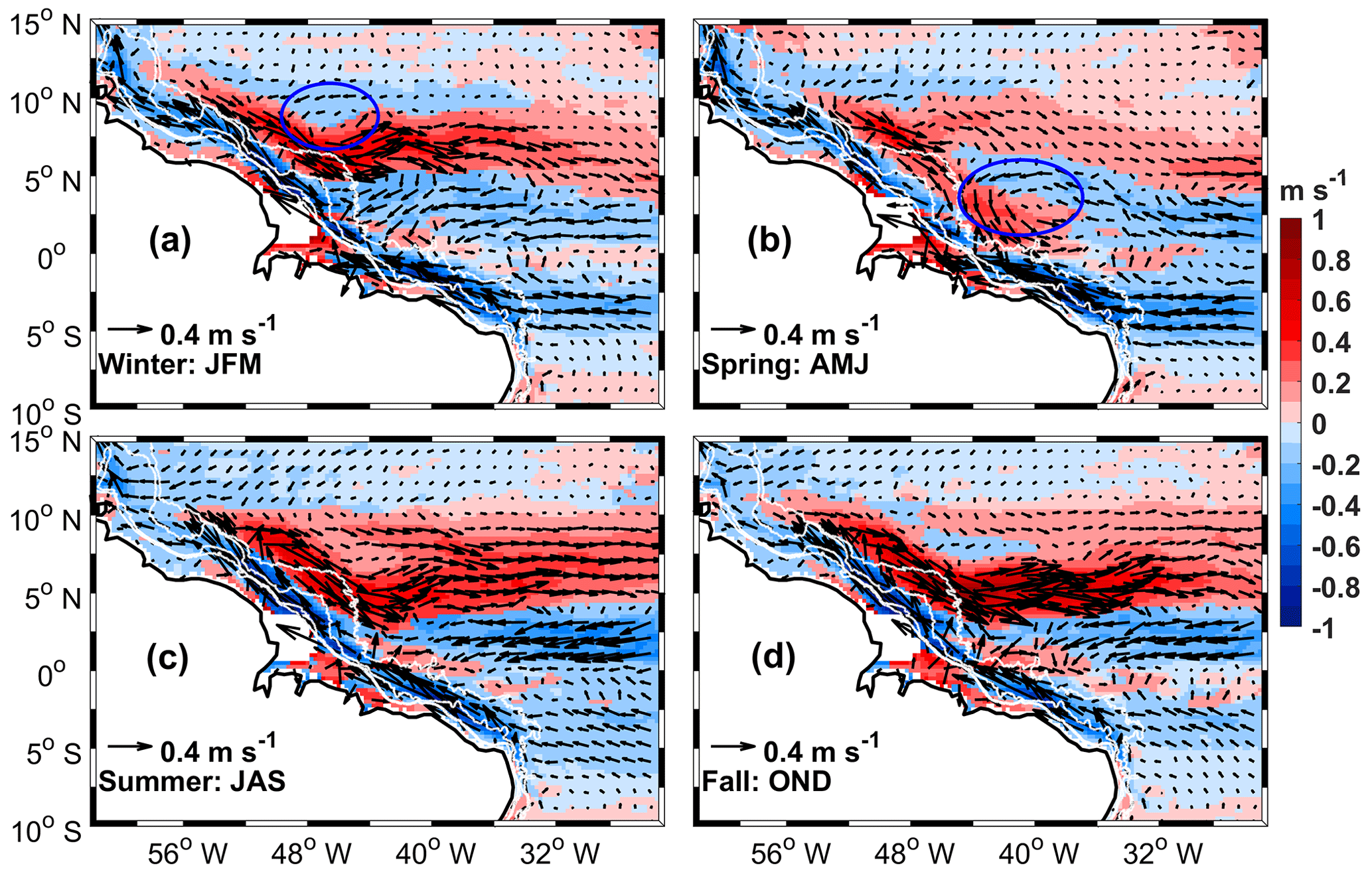
Figure 8 Seasonal maps of the geostrophic currents in the western tropical Atlantic over the 1993–2017 period for boreal winter (a JFM for January–February–March), boreal spring (b AMJ for April–May–June), boreal summer (c JAS for July–August–September), and boreal fall (d OND for October–November–December). The velocity vectors are superimposed onto the speed multiplied by the sign of their zonal components (m s⁻¹). The two cyclonic circulations observed during boreal winter and spring are indicated by blue ellipses. The white lines near the continent are from west to east, i.e., the 300, 1000, 3000, and 4000 m isobaths.

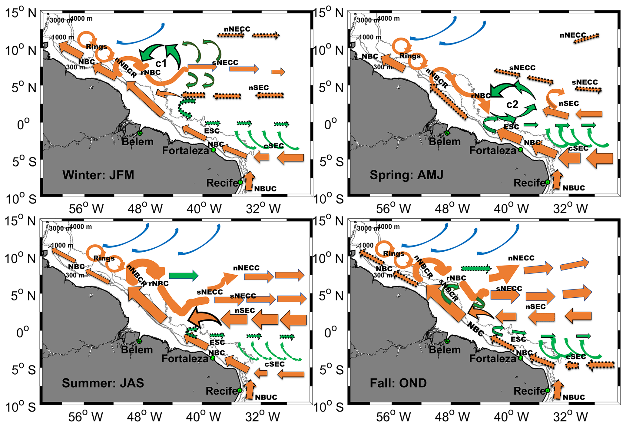
Figure 9 Schematic view of the seasonal maps of the tropical western boundary surface circulation together with the subsurface NBUC signature at the surface. C1 and C2 represent the cyclonic circulations highlighted in this study. The size of the arrows is wider when the intensity of the current is at its maximum (normal arrows) and decreases with season to reach its minimum (thin dotted line). The NBUC is represented because of its contribution to the NBC transport and is shown by dashed arrows. The current branches that are already known are in orange and blue (for the currents fed by Southern Hemisphere and Northern Hemisphere water, respectively). The green arrows characterize the new branches observed. NBC is the North Brazil Current, nNBCR and sNBCR are the northern and the southern flows of the North Brazil Current retroflection, respectively, rNBC is the retroflected branch of North Brazil current, nNECC and sNECC are the northern and the southern branches of the North Equatorial Countercurrent (NECC), respectively, cSEC and nSEC are the central and the northern branches of the South Equatorial Current (SEC), respectively, and ESC is the Equatorial Surface Current.

Finally, from all the analyses of the currents carried out above, we propose a new scheme for the seasonal variations of the western boundary tropical Atlantic circulation (Fig. 9). The new current branches found in this study are indicated in green and the currents coming from the north (south) are in blue (orange). The width of the current arrows is proportional to the intensity of the current, and the dotted arrows represent the currents with the minimum intensities. Several arrows are used for some currents to show their spatial variability. C1 and C2 are for the cyclonic circulations highlighted between 44–50 and 35–45^∘ W, respectively.

Concerning the interannual variability, Hormann et al. (2012), based on analyses of 17 years of altimetry and drifter data, found interesting scenarios regarding NECC spatial and temporal variability. However, they did not separate the sNECC from the nNECC. In their study, the authors have associated the strengthening of the NECC in the whole basin with the negative phase of the AZM and its northward shift with the positive phase of the AMM. Our results show the differing behaviors of the NECC system as a function of branch and core location. We also showed possible relationships between the southern NECC branch intensity and location with the AMM phases at 42^∘ W and conversely a possible relationship between the southern NECC branch intensity and location with the AZM phases at 32^∘ W. These results open the way to deeper investigations in future studies.

7 Summary and perspectives

A total of 25 years (1993–2017) of gridded altimetry data from CMEMS were used to improve the description of the seasonal and interannual variations of the western boundary circulation of the tropical Atlantic. To do so, a new approach based on the calculation of the current intensity was adopted, using six defined horizontal sections. These horizontal sections have been designed to intersect the path of the principal upper-ocean flows over the western tropical Atlantic. Copernicus Climate Service ERA5 wind estimates and the NOAA OI SST v2 product were also used to investigate the possible link between the variability of the regional circulation and the large-scale remote wind forcing and tropical Atlantic climate modes.

Our results highlight a complex regional circulation, with significant seasonal and year-to-year variations in current intensity and location. South of the Equator, we observe a stronger (weaker) cSEC and NBC during boreal spring (fall). North of the Equator, the NBC component flowing along the Guyana coast exhibits a similar annual cycle. However, between both components, the part of the NBC located before the retroflection is out of phase (i.e., stronger during summer–fall) when fed by the northern branch of the South Equatorial Current (nSEC). Its larger amplitudes appear during boreal fall, 3–4 months after the maximum of the remote wind stress curl (WSC) strength (in August). The North Equatorial Countercurrent (NECC) is connected with the retroflected branch of the NBC, and both show a similar annual cycle. A secondary North Brazil Current Retroflection (NBCR) was observed for the first time during boreal fall in this study: it is located between 4–6^∘ N. The two-core and branch structure of the NECC during the second half of the year was also confirmed and analyzed separately. Between 0–5^∘ N and 35–45^∘ W, a surface cyclonic circulation develops during boreal spring. It is found to initiate the growth of the NECC at 42^∘ W in June. However, at 32^∘ W, the NECC does not show any connection with this cyclonic circulation but starts its seasonal cycle earlier in April when the ITCZ migrates northward and the remote WSC strengthens. In the equatorial region, between 2^∘ S–2^∘ N, the geostrophic currents show the presence of an eastward Equatorial Surface Current (ESC), which has a seasonal cycle similar to the Equatorial Undercurrent (EUC). However, the ageostrophic velocities need to be considered here to fully understand the surface circulation.

The interannual variability is much weaker than the seasonal variability. It is more important in the eastern part of our study area, and there is no obvious regional pattern of low-frequency variations. The analysis of the changes in characteristics of the different current branches (intensity and core location) with respect to the tropical Atlantic climate modes shows different possible scenarios associated with one or both modes. It opens the way for further investigations concerning the link between the Atlantic climate modes (ACMs) and the current transports, which would not be possible with altimetry alone.

As a conclusion, this study demonstrates the ability of altimetry to characterize the seasonal and interannual variability of the surface circulation in the study area. It confirms previous findings but also significantly complements the knowledge of the different currents at regional scale. Combined use of regional modeling, altimetry, and in situ observations will allow us to go further in the understanding of the spatial and temporal structure of the regional circulation. The intraseasonal variability, significant in the near-shore region of the study area (Fig. 2d), is not studied here. It will be the subject of a future work based on a coastal altimetry product that will allow a significantly better resolution and accuracy along the continental shelf compared to a gridded product.

Appendix A: Acronyms and abbreviations

AMM	Atlantic Meridional Mode
AMOC	Atlantic meridional overturning circulation
AZM	Atlantic Zonal Mode
EUC	Equatorial Undercurrent
ITCZ	Intertropical Convergence Zone
NBC	North Brazil Current
rNBC	Retroflected branch of the NBC
NBCR	North Brazil Current retroflection
nNBCR	Northern NBCR flow
nNBCR lat	Latitude of the nNBCR maximum intensity
sNBCR	Southern NBCR flow
sNBCR lat	Latitude of the sNBCR maximum intensity
NECC	North Equatorial Countercurrent
nNECC	Northern branch of the NECC
nNECC lat	Latitude of the nNECC core
sNECC	Southern branch of the NECC
sNECC lat	Latitude of the sNECC core
PIRATA	Prediction and Research Moored Array in the
	Tropical Atlantic
SEC	South Equatorial Current
cSEC	Central branch of the SEC
nSEC	Northern branch of the SEC
VnNBCR	Value of the nNBCR maximum speed
VsNBCR	Value of the sNBCR maximum speed
VnNECC	Value of the nNECC core speed
VsNECC	Value of the sNECC core speed
ESC	Equatorial Surface Current
WSC	Wind stress curl
WSC neg max	Maximum negative WSC
WSC strength	WSC strength
WTA	Western tropical Atlantic