How subsurface and double-core anticyclones intensify the winter mixed-layer deepening in the Mediterranean Sea

The mixed layer is the uppermost layer of the ocean, connecting the atmosphere to the subsurface ocean through atmospheric fluxes. It is subject to pronounced seasonal variations: it deepens in winter due to buoyancy loss and shallows in spring while heat flux increases and restratifies the water column. A mixed-layer depth (MLD) modulation over this seasonal cycle has been observed within mesoscale eddies. Taking advantage of the numerous Argo floats deployed and trapped within large Mediterranean anticyclones over the last decades, we reveal for the first time this modulation at a 10 d temporal scale, free of the smoothing effect of composite approaches. The analysis of 16 continuous MLD time series inside 13 long-lived anticyclones at a fine temporal scale brings to light the importance of the eddy pre-existing vertical structure in setting the MLD modulation by mesoscale eddies. Extreme MLD anomalies of up to 330 m are observed when the winter mixed layer connects with a pre-existing subsurface anticyclonic core, greatly accelerating mixed-layer deepening. The winter MLD sometimes does not achieve such connection but homogenizes another subsurface layer, then forming a multi-core anticyclone with spring restratification. An MLD restratification delay is always observed, reaching more than 2 months in 3 out the 16 MLD time series. The water column starts to restratify outside anticyclones, while the mixed layer keeps deepening and cooling at the eddy core for a longer time. These new elements provide new keys for understanding anticyclone vertical-structure formation and evolution.

1 Introduction

The mixed layer corresponds to the ocean surface layer over which water properties are kept uniform through active mixing. It connects the atmosphere to the subsurface ocean through air–sea fluxes of heat, fresh water or other chemical components such as carbon (Takahashi et al., 2009; Large and Yeager, 2012). The mixed-layer depth (MLD) controls how deep the mixing acts, bringing water properties from below to the surface and the other way around. This depth is subject to pronounced seasonal variations, the mixed layer deepening with winter heat loss, while spring surface heating restratifies the column and the mixed layer gets shallower. Due to its importance for both ocean physics and biogeochemistry, global MLD climatologies were computed (de Boyer Montégut et al., 2004; Holte et al., 2017). Several MLD climatologies were also computed for the Mediterranean Sea (D'Ortenzio et al., 2005; Houpert et al., 2015), showing specific dynamics in winter convective regions such as the Gulf of Lion, the Aegean and the Adriatic seas, or the Rhodes gyre, with biological impacts on plankton bloom (D'Ortenzio and Ribera d'Alcalà, 2009; Lavigne et al., 2013). However large spread in MLD was also observed in regions hosting intense anticyclones such as the Algerian, Ionian and Levantine basins (Houpert et al., 2015), highlighting the need to take into account the local impact of mesoscale eddies.

Recent development of automatic eddy-tracking algorithms and eddy atlases (at a global scale, see for example Chelton et al., 2011, and Pegliasco et al., 2022; in the Mediterranean, see Stegner and Le Vu, 2019), combined with an increase of in situ measurements thanks to the development of autonomous platforms (Le Traon, 2013), recently allowed the influence of mesoscale oceanic eddies on the MLD to be studied. It is now well known that anticyclonic (respectively cyclonic) eddies tend to deepen (shoal) the MLD (Dufois et al., 2016; Hausmann et al., 2017; Gaube et al., 2019). Eddies actually amplify the MLD seasonal cycle, the deepest MLD anomaly being reached during winter (Hausmann et al., 2017; Gaube et al., 2019). A first mechanism was proposed by Williams (1988), the eddy modulation of the MLD being related to their induced sea surface temperature anomaly (SSTA). Indeed, as shown by Hausmann and Czaja (2012), anticyclonic (cyclonic) eddies are usually associated with positive (negative) SSTAs, and this is at least true in winter in the Mediterranean Sea (Moschos et al., 2022). It leads to stronger (weaker) heat loss during the winter and the triggering of enhanced (reduced) ocean convection and therefore deeper (shallower) MLD. In addition, Hausmann et al. (2017) and Gaube et al. (2019) found out that, for the Southern Ocean and global ocean respectively, the eddy MLD anomaly, computed from eddy composites, scales with the eddy sea surface height (SSH) amplitude. Gaube et al. (2019) proposed the same linear trend at the global scale ±1 m MLD anomaly for each 1 cm SSH for both cyclones and anticyclones. Physical drivers controlling the eddy-induced MLD are supported by other studies showing an eddy modulation of air–sea exchanges. Villas Bôas et al. (2015) found that ocean heat loss was enhanced (respectively reduced) in anticyclones (cyclones) in energetic regions of the South Atlantic Ocean, once again scaling with eddy amplitude, for both sensible and latent heat flux. Frenger et al. (2013) showed enhanced rainfall and cloud cover above anticyclones in the Southern Ocean as a consequence of enhanced turbulent heat fluxes but suggested a scaling with the eddy SSTA. Such a relation should remain coherent, as Hausmann and Czaja (2012) also found anticyclonic warm (cyclonic cold) eddy SSTAs to scale with the eddy amplitude in the Gulf Stream region. Altogether, eddy MLD anomalies are expected to be easily inferred provided that background measurements outside eddies are available, a promising link for remote sensing application.

However, all these studies were at a coarse monthly temporal resolution, whereas the mixed layer is driven by air–ocean fluxes and thus is expected to react at a timescale close to the inertial period (D'Asaro, 1985; Lévy et al., 2012). If several studies showed the MLD and upper-ocean stratification to vary over timescales of a week at regional scales (Lacour et al., 2019 in the North Atlantic or D'Ortenzio et al. (2021) in the Rhodes gyre), no studies are yet available on the temporal evolution of eddy MLD anomalies. A second limit in previous studies is the use of composite datasets that smooth out the non-linearities induced by eddies. If the composite analysis can provide a first-order trend, this is likely not sufficient to quantify accurately the various impacts of the wide diversity of individual eddies varying in size and intensity. A third but linked limit – explicitly pointed out by Villas Bôas et al. (2015) and Hausmann et al. (2017) – is their focus on surface-intensified eddies with the most coherent surface signature. Indeed, the relation between eddy SSTAs and SSH amplitude strongly relies on the hypothesis of a surface-intensified structure, and Assassi et al. (2016) showed that it should not be the case for subsurface anticyclones. Subsurface eddies are of a mesoscale structure where the density anomaly (compared to the outside-eddy density profile) is overlaid by an anomaly of opposite sign. For instance, a subsurface anticyclone has a lighter core at depth overlaid by a negative density anomaly near the surface. Following the thermal-wind equation, the depth of the maximal geostrophic speed is below the surface. The isopycnals and isotherms doming above a subsurface anticyclone core could greatly impact the upper-layer stratification and subsequently the inside-eddy mixed-layer dynamics. In the South China Sea and still using the composite method, He et al. (2018) found the anticyclones to be predominantly subsurface eddies. They also observed a linear trend between the subsurface temperature anomaly and SSH on an annual average and an eddy-induced MLD anomaly, but based on monthly climatology, and did not find a relationship with MLD. A more detailed comparison with more observational data and, in particular, a better temporal resolution is then lacking.

The Mediterranean Sea is an interesting region to study eddy influence on MLD. At first, due to repeated oceanographic campaigns, the density of in situ measurements is relatively high, and in particular, several campaigns specifically targeted long-lived mesoscale anticyclones in both western and eastern basins. Without aiming for exhaustiveness, one can list the following in particular: EGYPT (Taupier-Letage et al., 2010), BOUM (Moutin and Prieur, 2012), “Eye of the Levantine” (Hayes et al., 2011), PROTEVS (Garreau et al., 2018) and PERLE (Ioannou et al., 2019). Additionally, several Argo profiling floats were launched inside eddies and remained trapped for a long time (Ioannou et al., 2020), altogether allowing one to accurately follow particular eddies and to go beyond the averaged composite vision in the Mediterranean Sea. Moreover, data from these programmes were often only analysed in the scope of the campaigns, and an eddy study with a larger statistical focus is still lacking. A second relevance for Mediterranean eddies is the variety of mesoscale structures in terms of dynamics, from intense Algerian and Ierapetra anticyclones needing cyclogeostrophic corrections (Ioannou et al., 2019) to subsurface eddies with strong density anomalies but weak SSH signatures (Hayes et al., 2011). Moutin and Prieur (2012) also showed the vertical structure, in temperature and salinity, of mesoscale eddies to be very different from one basin to another. Barboni et al. (2021) showed the marked subsurface difference between a new anticyclone detached from the coast compared to an offshore structure having been tracked for more than a year. All these structures should provide different examples of eddy–MLD interactions.

In the Mediterranean Sea, there is additionally a strong asymmetry between cyclones and anticyclones, remarkable in terms of lifetime difference (Mkhinini et al., 2014). The deformation radius in the Mediterranean Sea is indeed about 8 to 12 km (Kurkin et al., 2020), and cyclones are less stable when greater than the deformation radius and more subject to external shear (Arai and Yamagata, 1994; Graves et al., 2006). This leads to cyclones being predominantly below the effective resolution of SSH products by about 20 km (Stegner et al., 2021). As a consequence, anticyclones are coherent larger vortices, while cyclones in the Mediterranean Sea, as detected by altimetry, are instead cyclonic gyres bounded by topography or hydrographic fronts such as the Ligurian, southwestern Crete or Rhodes gyre (Stegner et al., 2021). MLD evolution inside these cyclonic gyres was already surveyed because of their importance for biological production, in particular with the development of BGC-Argo (D'Ortenzio et al., 2021; Taillandier et al., 2022). Apart from specific campaigns, Mediterranean anticyclones remain poorly analysed despite being more coherent, and statistical comparison based on vertical profiles is lacking, with the noticeable exception of the Biogeochemistry from the Oligotrophic to the Ultraoligotrophic Mediterranean (BOUM) campaign surveying three anticyclones across the Mediterranean in 2008 (Moutin and Prieur, 2012).

This paper aims to study the temporal evolution of the mixed layer inside a wide diversity of long-lived anticyclones in the Mediterranean Sea compared to the evolution of the background MLD. The goal is to quantify more precisely the local impacts of individual eddies on the winter mixed-layer deepening. The paper is organized as follows. Section 2 describes the eddy detection and tracking algorithm and the in situ profile database. Section 3 details the methodology used to compute the MLD and to colocalize profiles and eddies in order to quantify accurately the MLD anomalies induced by individual eddies. In Sect. 4, we analyse the MLD evolution at anticyclone cores, provide statistical analysis over the variety of structures surveyed and discuss the impact of complex vertical eddy structures on winter mixed-layer deepening. Finally, in Sect. 5, we discuss the possible physical drivers and implications of these MLD anomalies.

2 Data

2.1 Anticyclone detections: the DYNED-Atlas

Eddy detections are provided through the angular momentum eddy detection and tracking algorithm (AMEDA). AMEDA is a mixed velocity–altimetry approach; it relies on using primarily streamlines from a velocity field and identifying possible eddy centres computed as maxima of local normalized angular momentum (Le Vu et al., 2018). It was successfully used in several regions of the world ocean using altimetric data (Aroucha et al., 2020; Ayouche et al., 2021; Barboni et al., 2021), high-frequency radar data (Liu et al., 2020) or numerical simulations (de Marez et al., 2021). From 1 January 2000 to 31 December 2019, AMEDA was applied on the Archiving, Validation and Interpretation of Satellite Oceanographic data (AVISO) sea surface height (SSH) delayed-time product at a resolution of $\mathrm{1}/\mathrm{8}$^∘ with daily output. From 1 January 2020 to 31 December 2021, AMEDA was applied on the AVISO SSH near-real-time day + 6 product (Pujol, 2021) at the same spatial and temporal resolutions. In each eddy single observation (one eddy observed one day), AMEDA gives a centre and two contours. The “maximal speed” contour is the enclosed streamline with maximal speed (i.e. in the geostrophic approximation, with maximal SSH gradient); it is assumed to be the limit of the eddy core region where water parcels are trapped. The “end” contour is the outermost closed SSH contour surrounding the eddy centre and the maximal speed contour; it is assumed to be the area of the eddy footprint, larger than just its core but still influenced by the eddy shear (Le Vu et al., 2018). AMEDA gathers eddy observations in eddy tracks, allowing the same structure to be followed in time and space, sometimes over several months. The eddy track collection in the whole Mediterranean Sea constitutes the DYNED-Atlas database (Stegner and Le Vu, 2019), which is available online (for the years 2000 to 2019) at https://www1.lmd.polytechnique.fr/dyned/, last access: 21 February 2023. From 2000 to 2021, a total of 7038 (respectively 8890) anticyclonic (cyclonic) eddy tracks were retrieved. The asymmetry in eddy numbers is driven by a lifetime difference, with anticyclones living noticeably longer, an asymmetry even more marked in the Levantine Basin (Barboni et al., 2021).

2.2 In situ profiles

A climatological database is created collecting in situ profiles from the Coriolis Ocean Dataset for Reanalysis (CORA). Delayed-time (CORA-DT; Szekely et al., 2019b) profiles are recovered from 2000 to 2019 (113 486 profiles), and near-real-time (Copernicus-NRT; Copernicus, 2021) profiles are recovered from 2020 to 2021, included using the “history” release (22 821 profiles). These datasets are multi-platform, gathering in situ vertical measurements from conductivity–temperature–depth (CTD) casts, expendable bathythermograph (XBT) measurements (mostly before 2008), Argo floats (mostly after 2005, with a strong increase after 2012) and gliders (mostly after 2008), enabling an average of 10 000 profiles available per year from 2011 onwards. In addition, some profiles prior to 2020 have not yet been released in CORA-DT but are available in Copernicus-NRT. This happens in particular when the salinity sensor of an Argo float has abnormal values but the temperature is still correct (by visual inspection and correct quality flag). As the MLD computation can be performed on a temperature profile alone, profiles were also retrieved in NRT mode after careful checking, as described in Appendix A. This provides an extra 20 746 profiles from 2000 to 2019. Spotted duplicates between CORA-DT and Copernicus-NRT are retrieved only from CORA-DT. The complete database then accounts for 157 053 profiles in total, with the following platform distribution: 8596 CTDs, 11375 XBTs, 60 019 Argo, 76 967 glider profiles and 96 unspecified and is available at https://doi.org/10.17882/93077 (Barboni et al., 2023).

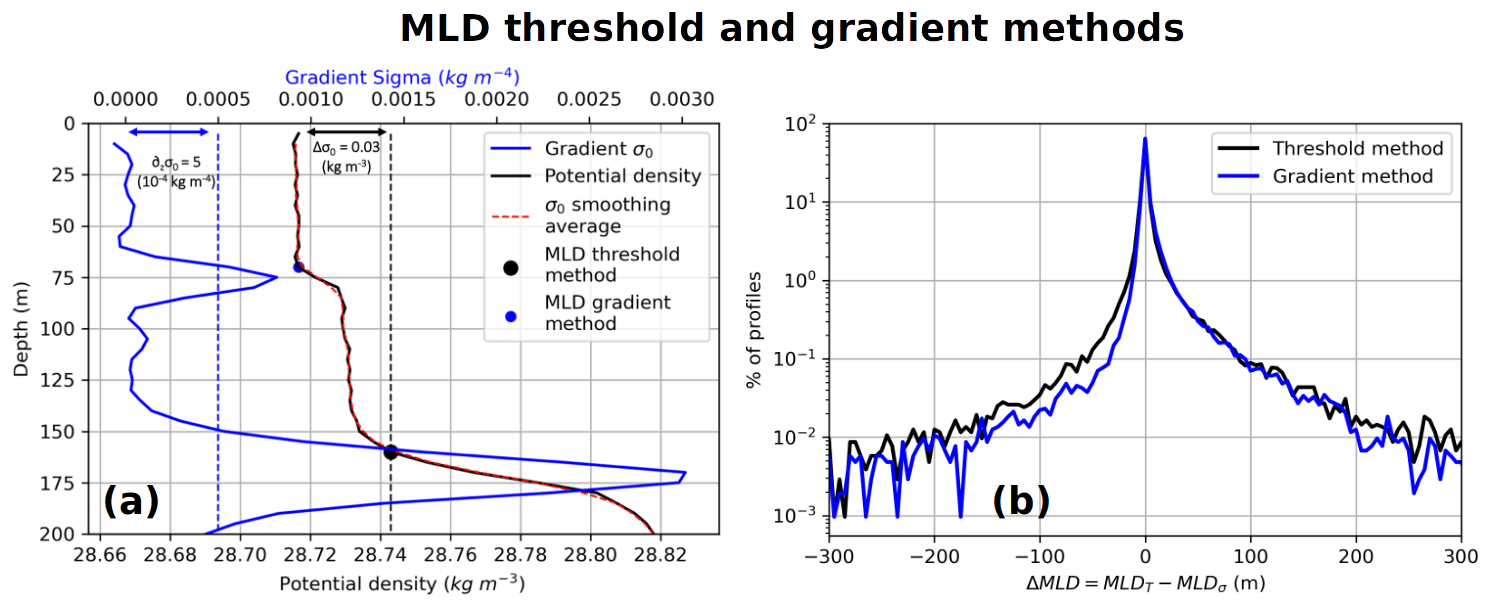
Figure 1 (a) MLD detection on one potential density profile with our gradient method (blue dot) and threshold method (black dot); (b) fraction of the profiles as a function of ΔMLD for the threshold (black line) and gradient (blue line) method.

3 Methods

3.1 MLD computation

The global analysis conducted by de Boyer Montégut et al. (2004) led to MLD being detected by threshold values of 0.03 kg m⁻³ for density and 0.2 ^∘C for temperature, based on a reference depth of 10 m to avoid diurnal heating at the surface. In the Mediterranean Sea, D'Ortenzio et al. (2005) used this methodology for a 0.5^∘-resolution MLD climatology. Houpert et al. (2015) updated it with 8 supplementary years of data but opted for a 0.1 ^∘C temperature threshold. This more restrictive criterion enables the reduction of the difference between the MLD computed on temperature profiles and the one computed on density profiles. Gradient methods look in a similar way for critical gradients as an indicator of the mixed-layer base. Typical gradient threshold values in use are $\mathrm{2.5}\times {\mathrm{10}}^{-\mathrm{2}}$ ^∘C m⁻¹ for temperature profiles and range from $\mathrm{5}\times {\mathrm{10}}^{-\mathrm{4}}$ to $\mathrm{5}\times {\mathrm{10}}^{-\mathrm{2}}$ kg m⁻⁴ for potential density profiles (Dong et al., 2008). Mixed gradient and threshold methods were also developed (Holte and Talley, 2009). Here, we aim to capture as accurately as possible the MLD evolution, which can vary on timescales shorter than a month. More specifically, we observed in several cases that the threshold method (with criteria Δσ=0.03 kg m⁻³ and ΔT=0.1 ^∘C) can miss the mixed layer and return the main thermocline instead (see Fig. 1a). The main thermocline is indeed characterized by a small jump in potential density (or in temperature) but a significant peak in the gradient profile, and it happens mostly in the spring, probably due to a start of restratification that quickly becomes mixed. To capture such small-scale restratification events, we built the following methodology, combining both threshold and gradient approaches. Using the thresholds Δσ=0.03 kg m⁻³ and ΔT=0.1 ^∘C, we derive a first estimate of the MLD. If it is shallower than 20 m, we take it as our estimate of the MLD. Otherwise, we apply a three-point running average to remove small spikes and to compute the gradient using a second-order centred difference. From the subsurface (20 m) up to the first MLD estimate, we apply a gradient method with the given gradient thresholds: $\left|{\partial }_z\mathit{\sigma }\right|>\mathrm{5}\times {\mathrm{10}}^{-\mathrm{4}}$ kg m⁻⁴ or $\left|{\partial }_{z}T\right|>\mathrm{2.5}\times {\mathrm{10}}^{-\mathrm{3}}$ ^∘C m⁻¹. If the gradient fails to exceed the threshold within the given depth range, then the first MLD estimate is kept.

Threshold and gradient methods are limited by their dependence on the criterion values which can have strong influence on the MLD estimate. The relatively low gradient thresholds chosen here appeared to be necessary to catch the MLD in some of our profiles, as higher thresholds would return the main thermocline (see Fig. 1a). A sample of 400 randomly picked profiles collocated inside eddies was used for validation. We chose this validation dataset with profiles inside eddies because it is our main focus. Wrong detection on double-gradient profiles inside eddies was found to be quite large, sometimes exceeding 100 m. On these 400 profiles, 22 (5.5 %) of them were identified as double-gradient profiles, resulting in an overestimated MLD when derived with the threshold method. Moving to our methodology, this issue is now only encountered for two profiles (0.5 %). However, with the gradient method comes some issues for profiles with small residual spikes despite the applied smoothing. For two profiles, the gradient method returned wrong MLD detection where the threshold method was correct. However, the gradient method was found overall to be more accurate for estimating the MLD.

Moreover, the chosen thresholds should return similar estimates between an MLD obtained from a temperature profile (MLD_T) and one obtained from a potential-density profile (MLD_σ). Potential density is a better estimate of the stability of a layer, and thus MLD_σ should give a more reliable value. However, salinity (and hence density) suffers from data holes, representing about 15 % in our dataset. Temperature profiles then offer a good alternative in evaluating the MLD, providing MLD_T gives a estimate to that of MLD_σ. An MLD_T and MLD_σ difference histogram is shown in Fig. 1b: the gradient method appears to reduce this difference slightly, with 64 % of the profiles leading to the same estimate and 94 % to less than a 30 m difference compared to 62 % and 93 % respectively for the threshold method. MLD is then computed on the density profile or, if no density is available, on the temperature profile.

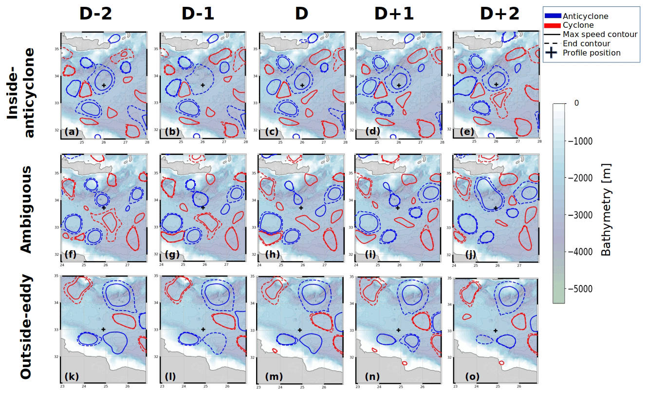
Figure 2 Profile colocalization with eddy contours for an “inside-anticyclone” profile (a–e), an “ambiguous” profile (f–j) and an “outside-eddy” profile (k–o). Profile cast position is assumed to be fixed and is compared to eddy contours at D−2, D−1, D, D+1 and D+2, D being the profile cast date.

3.2 Eddy colocalization and background estimate

In order to characterize the impact of anticyclonic eddies on the MLD seasonal evolution and spatial gradient, we need to accurately colocalize in situ profiles with eddy observations. However, due to altimetric product interpolation and disparate satellite tracks, SSH-based contours can vary a lot in size and position, making a single eddy observation less reliable in the Mediterranean Sea (Amores et al., 2019; Stegner et al., 2021). Therefore, we colocalize eddy observations and in situ profiles at ±2 d. Assuming a profile position fixed at cast date D, it is then labelled as “inside-eddy” if it remains inside the maximal speed contours of the same eddy at D−2, D−1, D, D+1 and D+2 (at least four contours out of five). This four-out-of-five threshold avoids the neglect of a collocated profile when the eddy contour is not available for just one day (see Fig. 2b). For the same purpose, hereafter, the eddy centre and the distance of a profile to the eddy centre are averaged at ±2 d.

AMEDA also gives, for each observation, the last closed SSH contour (see Sect. 2.1), inside which there is still an impact by the eddy shear, but outside of the maximal speed contour, the water particles are not assumed to be trapped. The area between the maximal speed and last closed SSH contours is then considered to be an intermediate zone to be discarded. Consistently with the “inside-eddy” definition, we label as “outside-eddy” only the profiles that stay outside any eddy contours at ±2 d of its cast date. Any profile being neither “inside-” nor “outside-eddy” is considered to be ambiguous and is discarded. From 2000 to 2021, out of 157 053 profiles retrieved in the Mediterranean Sea, 104 787 are labelled “outside-eddy”, 7939 are “inside-anticyclone” and 14 919 are “inside-cyclone”; the remaining 29 410 “ambiguous” profiles are removed from this analysis. This asymmetry between anticyclones and cyclones sampling is also due to heterogeneous oceanographic surveys (Houpert et al., 2015), particularly the numerous glider missions in the Gulf of Lion, a cyclonic gyre with no large anticyclones (Millot and Taupier-Letage, 2005). Figure 2 illustrates the colocalization method detailed above with three examples: an “inside-anticyclone” profile (Fig. 2a–e), an “ambiguous” one (Fig. 2f–j) and an “outside-eddy” one (Fig. 2k–o). For this particular “inside-anticyclone” profile, the maximal speed contour was missing at day D−1 but was available for the other days, and the profile was indeed cast close to the eddy centre.

To follow the accurate evolution of the MLD inside anticyclones, we need a reference for comparison: an unperturbed, local and time-coincident ocean state without eddies, hereafter called “background”. This outside-eddy background differs from a classical climatology used in previous studies (Gaube et al., 2019) by the removal of the eddy mean effect and by avoiding time averaging as much as possible. The background of an eddy, at a given time t and centre position C(t), is then constituted by the mean of all profiles labelled as outside-eddy that are closer than 250 km to C(t), cast within $\mathrm{\Delta }\mathrm{day}=\pm \mathrm{10}$ d of the same year or of the previous or the following year ($\mathrm{\Delta }y=\pm \mathrm{1}$ year). For example, when computing the corresponding background of an eddy around 15 February 2018, the background encompasses profiles that are labelled as outside-eddy, are closer than 250 km, and are cast from 5 to 25 February 2017, 2018 and 2019. A threshold on the number of profiles is required: if fewer than 10 profiles meet the distance, time and outside-eddy requirements, then no background is computed. At last, we define the “background MLD” to be the median MLD of the profiles constituting the background. Computing the median is preferred to the mean, as the MLD distribution is not centred but skewed downwards. This computation is performed for each time step with a temporal resolution of 5 d. As shown in Appendix (Fig. A1), with the test case of the Ierapetra anticyclone taking place over 2 years (corresponding events “IER1–2” on Table 1 and Fig. 10), the background MLD is not highly sensitive to the choice of Δday and Δy. The background MLD evolution is indeed similar, with Δday = 10, 15 or 20 d and $\mathrm{\Delta }y=\mathrm{0},\mathrm{1}$ or 2 years. It is, however, important not to take all years, as interannual variability then starts to smooth the background MLD evolution. On the other hand, taking only profiles of the same year (Δy=0) sometimes translates into not having enough profiles to have a background estimate (see Fig. A1a). We therefore chose Δday = 10 d and Δy=1 year as day and year intervals in order to capture MLD variations that are as short as possible, which is crucial for parameters that vary quickly, such as the MLD. For the two earliest recorded events (Mersa Matruh 1 and 2 in 2006 and in 2008; see Table 1), Δy is set to 2 years because no background MLD was available otherwise. Choosing Δy=1 allows one to have accurate eddy-induced anomalies without them being corrupted by interannual variability of temperature and salinity fields, which can be marked in the Mediterranean, particularly in the eastern basin (Ozer et al., 2017). A significant warming trend is also observed (Parras-Berrocal et al., 2020).

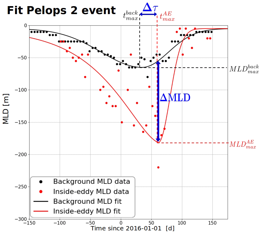
Figure 3 Detail of winter deepening event Pelops (PEL) 2 in 2016 (see Table 1 for details). Anticyclonic core MLD data are shown as red dots, and background MLDs are shown as black dots, with time steps of 5 d. MLD fit is shown as a red line for the anticyclonic core (see Eq. 2) and as a black line for background MLD (see Eq. 1).

3.3 MLD evolution function fit

To describe more objectively the MLD seasonal evolution in the background, we performed a function fit using the Python optimization routine scipy.optimize.curve_fit. MLD data points are selected according to 5 d time steps. Background MLD is fitted by a skewed Gaussian, $t_{\max }^{\mathrm{back}}$ being the time when the deepest MLD (MLD${}_{\max }^{\mathrm{back}}$) is reached; σ and τ are respectively the restratification and deepening timescales:

$$\begin{array}{}\text{(1)}& \begin{array}{ll}f\left(t\right)={\mathrm{MLD}}_{\max }^{\mathrm{back}}\exp \left(-\frac{{\left(t-t_{\max }^{\mathrm{back}}\right)}^{\mathrm{2}}}{\mathrm{2}{\mathit{\tau }}^{\mathrm{2}}}\right)& \text{if}t<t_{\max }^{\mathrm{back}},\\ f\left(t\right)={\mathrm{MLD}}_{\max }^{\mathrm{back}}\exp \left(-\frac{{\left(t-t_{\max }^{\mathrm{back}}\right)}^{\mathrm{2}}}{\mathrm{2}{\mathit{\sigma }}^{\mathrm{2}}}\right)& \text{otherwise}.\end{array}\end{array}$$

This fit captures the background MLD evolution, somehow smooth, typically with a sharper restratification than deepening (τ<σ). However, this is not sufficient for the anticyclonic core MLD evolution that can have more abrupt variations, then calling for a more complex fit with two deepening timescales τ₁ and τ₂:

$$\begin{array}{}\text{(2)}& \begin{array}{lll}f\left(t\right)& =& \left({\mathrm{MLD}}_{\max }^{\mathrm{AE}}-B\right)\exp \left(\frac{t-t_{\max }^{\mathrm{AE}}}{{\mathit{\tau }}_{\mathrm{1}}}\right),\\ & +& B\exp \left(\frac{t-t_{\max }^{\mathrm{AE}}}{{\mathit{\tau }}_{\mathrm{2}}}\right)\text{if}t<t_{\max }^{\mathrm{AE}}\\ f\left(t\right)& =& {\mathrm{MLD}}_{\max }^{\mathrm{AE}}\exp \left(-\frac{{\left(t-t_{\max }^{\mathrm{AE}}\right)}^{\mathrm{2}}}{\mathrm{2}{\mathit{\sigma }}^{\mathrm{2}}}\right)\text{otherwise}.\end{array}\end{array}$$

To fit the MLD evolution accurately, and particularly to have the maximal depth reached, data are fitted with weights proportional to their depth. Because it is difficult to have long and continuous time series, data are often missing for the previous or next summers. To ensure physical behaviour, fit is forced back to 10 m on the edges, miming summer stratification. The MLD anomaly (MLD^anom) is defined as the difference between the fitted background and anticyclonic core MLD. MLD^anom is a function of time but reaches its maximum (ΔMLD) at almost the same time as the absolute anticyclonic core MLD, as the latter has more amplitude than the background one. At last, an advantage of the scipy.optimize.curve_fit routine is that it provides the parameter covariance matrix and hence an error estimate, taking the square root of the covariance matrix diagonal (Bevington et al., 1993). It can happen that the covariance matrix has very large values – in this case, we used an upper uncertainty of ±30 m for ΔMLD and ±20 d for $t_{\max }^{\mathrm{AE}}$. A fit illustration is provided in Fig. 3 for the Pelops 2 event in 2016 (see Table 1), with the real MLD as dot data and the fits as continuous lines and with the background in black and the anticyclonic core in red. Using the fit routine, maximal MLD anomaly is then estimated as $\mathrm{\Delta }\mathrm{MLD}=\mathrm{127}\pm \mathrm{13}$ m for this event. One can also notice an absence of coincidence between the deepest inside-eddy and background MLDs. Following previous notation, we can then define a restratification delay of the anticyclonic core MLD, which is used throughout this study: $\mathrm{\Delta }\mathit{\tau }=t_{\max }^{\mathrm{AE}}-t_{\max }^{\mathrm{back}}$. In the example shown in Fig. 3, $\mathrm{\Delta }\mathit{\tau }=\mathrm{26}\pm \mathrm{11}$ d.

4 Results

Several long-lived anticyclones are tracked for several months, recording up to 16 winter mixed-layer deepening events at their core. In order to investigate the relation between the MLD evolution and the vertical eddy structure, we plot together the time series of MLD and vertical temperature gradients inside the eddy core. Two different MLD temporal patterns are observed, depending on whether or not the current winter mixed layer reaches the subsurface anticyclone core. This core is constituted by a pre-existing homogeneous layer, and in the following, we define as “homogenized” a layer with a temperature gradient constantly below $\mathrm{2.5}\times {\mathrm{10}}^{-\mathrm{3}}$ ^∘C m⁻¹ in absolute value.

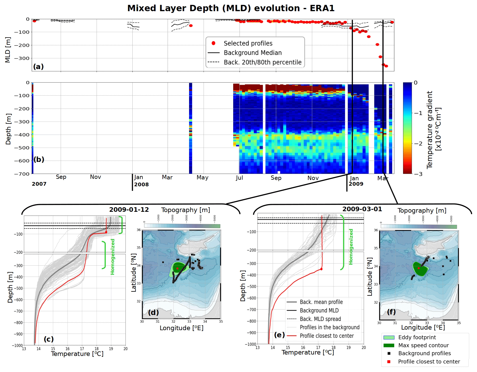
Figure 4 In-depth evolution of an Eratosthenes anticyclone, listed as “ERA1” in Table 1. (a) MLD evolution, with continuous black line for background MLD (and dashed line for associated spread between 20th and 80th percentiles) and red dots for the anticyclonic core MLD closest to eddy centre. (b) Time series of inside-eddy temperature gradient, blue showing homogeneous and red showing stratified layers; (c) (respectively e) shows vertical profiles around 12 January 2009 (1 March 2009) with background profiles in thin grey lines, background mean as thick grey line, inside-eddy profile as red line, a red dot highlighting anticyclonic core MLD and a green bar indicating homogenized layers (temperature gradient below $\mathrm{2.5}\times {\mathrm{10}}^{-\mathrm{3}}$ ^∘C m⁻¹). Horizontal continuous and dashed black line refer back to background MLD and spread from panel (a); (d) (respectively f) shows profiles' corresponding position on a map with same colour code together with the eddy maximal-speed contour (dark green shape) and eddy footprint (outermost closed SSH contour, light green shape). Bathymetric data are from ETOPO1 (Smith and Sandwell, 1997).

4.1 Winter deepening connecting pre-existing subsurface core

A very deep mixed layer can be observed in several anticyclones when the MLD erodes the inside-eddy stratification and abruptly connects with a subsurface homogenized core, an event hereafter called a “connecting” MLD. An example of this evolution is described below with a long-lived Eratosthenes anticyclone during winter 2008–2009. Its temporal evolution from August 2007 to April 2009 is shown in Fig. 4 and is listed hereafter and in Table 1 with the name “Eratosthenes (ERA) 1”. This kind of anticyclone, also called “Cyprus eddy” or even “Shikmonah gyre”, are large mesoscale structures with an almost stationary position south of the island of Cyprus in the Levantine Basin, extensively studied with several CTDs (Brenner, 1993; Krom et al., 1992; Moutin and Prieur, 2012), gliders and Argo float deployments (Hayes et al., 2011). The anticyclonic density anomaly is characterized, on average, by a deep (about 400 m) and extremely warm temperature anomaly (up to +2 ^∘C at 400 m) (Moutin and Prieur, 2012; Barboni et al., 2021), sometimes with a strong salt anomaly (Hayes et al., 2011). Thus temperature profiles are considered to be a good estimate for the relative density and temperature gradient for stratification.

An Argo float remained trapped inside this anticyclone from mid-2008 to the death of this eddy in early 2009, allowing an MLD deepening event during winter 2008–2009 to be captured well. An inside-anticyclone profile is shown at the beginning (12 January 2009; Fig. 4c) and the end (1 March 2009; Fig. 4e) of the winter. First, one can notice that the anticyclone vertical structure in January 2009 is constituted by a subsurface homogenized layer from 100 to 300 m, which can be tracked from July 2008 on the stratification time series (Fig. 4b) and was likely formed by convection in the previous winter. The anticyclone core profile in Fig. 4c indeed has a marked temperature anomaly on the order of +2 ^∘C at 450 m compared to the background, proving they indeed sample the eddy core. Some profiles with a very warm temperature at 400 m deep are misleadingly considered to be outside-eddy but do not corrupt the mean background (thick grey line). MLD is also deeper inside the Eratosthenes anticyclone: the anticyclonic core MLD is 90 m deep, while it is around 60 m in the background. The deeper homogenized core remains unmixed below a seasonal thermocline: +1 ^∘C temperature jump at 100 m in Fig. 4c. Later, the winter cooling and subsequent MLD deepening eroded this stratification inside the anticyclone, as shown by the temperature gradient vanishing in the upper 100 m, and the winter MLD connected with the primitive core and mixed with it in February 2009 (Fig. 4b). Then on 1 March 2009 (Fig. 4e), the anticyclone core profile measured an MLD reaching 350 m.

Inside- and outside-eddy MLD temporal evolutions noticeably do not coincide: on MLD time series (Fig. 4a), background MLD shoaled from the end of January, whereas inside-eddy MLD continued to deepen. Then on 1 March 2009, most background profiles started to restratify, with temperature gradients in the upper 100 m (thin grey lines in Fig. 4e), while anticyclonic core MLD rose back to about 20 m only in late March 2009 (Fig. 4a). This restratification, occurring at a different time outside- and inside-eddy, with a delay of about 2 months, leads to the noticeable situation measured on 1 March 2009: the inside-anticyclone profile is warmer than its environment at depth (100 to 350 m deep) but is homogenized in its upper part, whereas background profiles are stratified with positive temperature gradients. Such geometrical configuration leads to an anticyclone negative temperature (and hence positive density) anomaly from 50 m to the surface compared to the stratified outside-eddy profile. Such a positive density anomaly above the eddy core is then a clear signature of a subsurface anticyclone (Assassi et al., 2016).

Over the whole 2008–2009 winter, background MLD barely reached 60 m, whereas the anticyclonic core MLD went down to 350 m. This intense deepening at the anticyclone core is due to the pre-existing subsurface eddy, made of a well-mixed layer at a depth of a few hundred metres below the summer stratification. When the winter mixed layer deepens, it reconnects to this deep subsurface core and leads to a rapid and strong MLD increase in comparison to the eddy background. This MLD temporal pattern is characteristic of a “connecting” event, observed 10 times in our analysis and throughout the Mediterranean Sea (see Sect. 4.3).

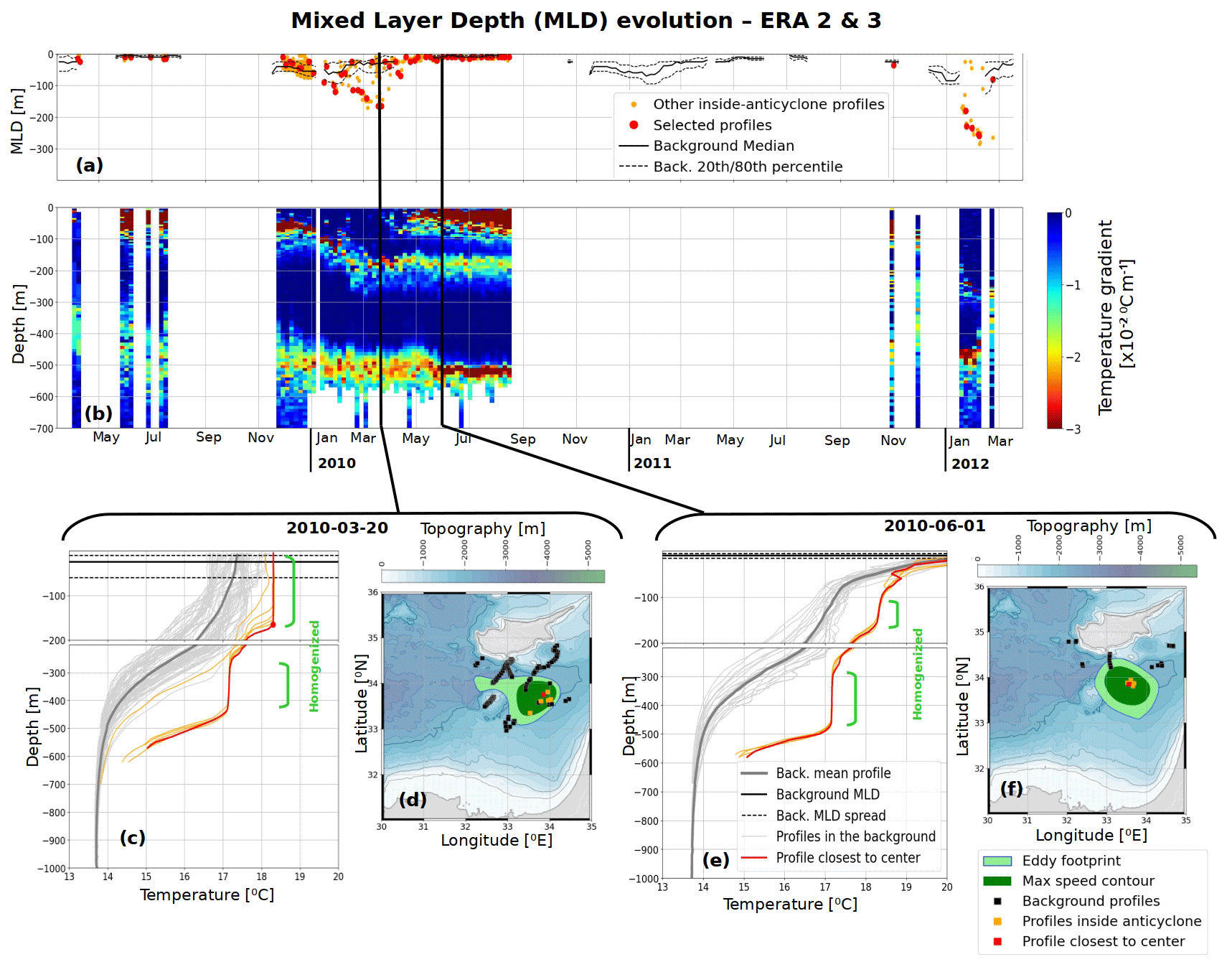
Figure 5 Same colour codes and legend as in Fig. 4. In panels (a), (c) and (e), orange lines and dots show additional inside-eddy profiles and corresponding MLD, but these are further away from the eddy centre than the selected one shown in red.

4.2 Winter deepening not connecting pre-existing subsurface core

Conversely, for some other anticyclones, it can clearly be seen that the subsurface temperature anomaly does not connect with the winter mixed layer and remains unperturbed and homogenized at depth. Such an event is hereafter called a “non-connecting” MLD. Figure 5 shows the evolution of another Eratosthenes anticyclone living from 2009 to early 2012, with two recorded anticyclonic core MLD deepenings in 2010 and 2012 (respectively listed in Table 1 as“ERA2” and “ERA3”), with same colour codes as in Fig. 4, with profiles on 20 March 2010 and 15 June 2010. As several profiles were located at the same time inside the anticyclone, they are shown with the orange line in Fig. 5c and e (respectively orange dot for MLD in Fig. 5a). The red line highlights only the profile with the closest distance to the eddy centre, assumed to be more representative of the eddy core.

Similarly to the “ERA1” event in 2009 described above, a thick and deep subsurface anomaly forms a primitive eddy core in late 2009 as a homogeneous layer from 250 to 400 m deep (green bar on Fig. 5c), reaching an anomaly of about +2.5 ^∘C at 400 m. However, the anticyclonic-core MLD did not deepen below 150 m in the winter 2009–2010, only forming a second homogeneous layer above. This constitutes a second surface core, still separated from the primitive core by a temperature stratification, revealed by a temperature gradient continuous in time (Fig. 5b). On the vertical profile on 20 March 2010 (Fig. 5c), a temperature jump of about 1 ^∘C remains between the two cores, forming a double-core anticyclone. In June 2010 (Fig. 5e), this second homogeneous layer is itself covered by the spring restratification, then forming what is also referred to as “thermostad” or “mode-water eddy” in the literature (Dugan et al., 1982). Thanks to the trapped Argo floats remaining near the eddy core for months, both cores could be tracked until August 2010 as separated in the subsurface.

Such “non-connecting” winter MLD inside anticyclone reveals the possibility of a persisting separation between a primitive subsurface anticyclone core and the new homogeneous layer formed by the current winter mixing, then constituting a double-core anticyclone. The example showed in Fig. 5 occurred on an Eratosthenes anticyclone, in the same region as the anticyclone in which a “connecting” MLD example was previously shown in Fig. 4. This MLD pattern is not limited to this example and was also observed five times in other regions, as detailed in the next section. Consequences of the formation of a double-core anticyclone are discussed in Sect. 5.2 hereafter, with another remarkable example in Fig. 10.

Figure 6 Map of well-sampled winter mixed-layer deepening events inside anticyclones listed in Table 1. Big dots show “connecting” events, while crosses show “non-connecting” ones. Colour depends on the region: Central Tyrrhenian (TYR), Pelops (PEL), Ierapetra (IER), Mersa Matruh (MM) and Eratosthenes (ERA, also called “Cyprus”). Isobaths shown on the maps are at 100, 500, 1000 and 1500 m depth; topographic data from ETOPO1 (Smith and Sandwell, 1997).

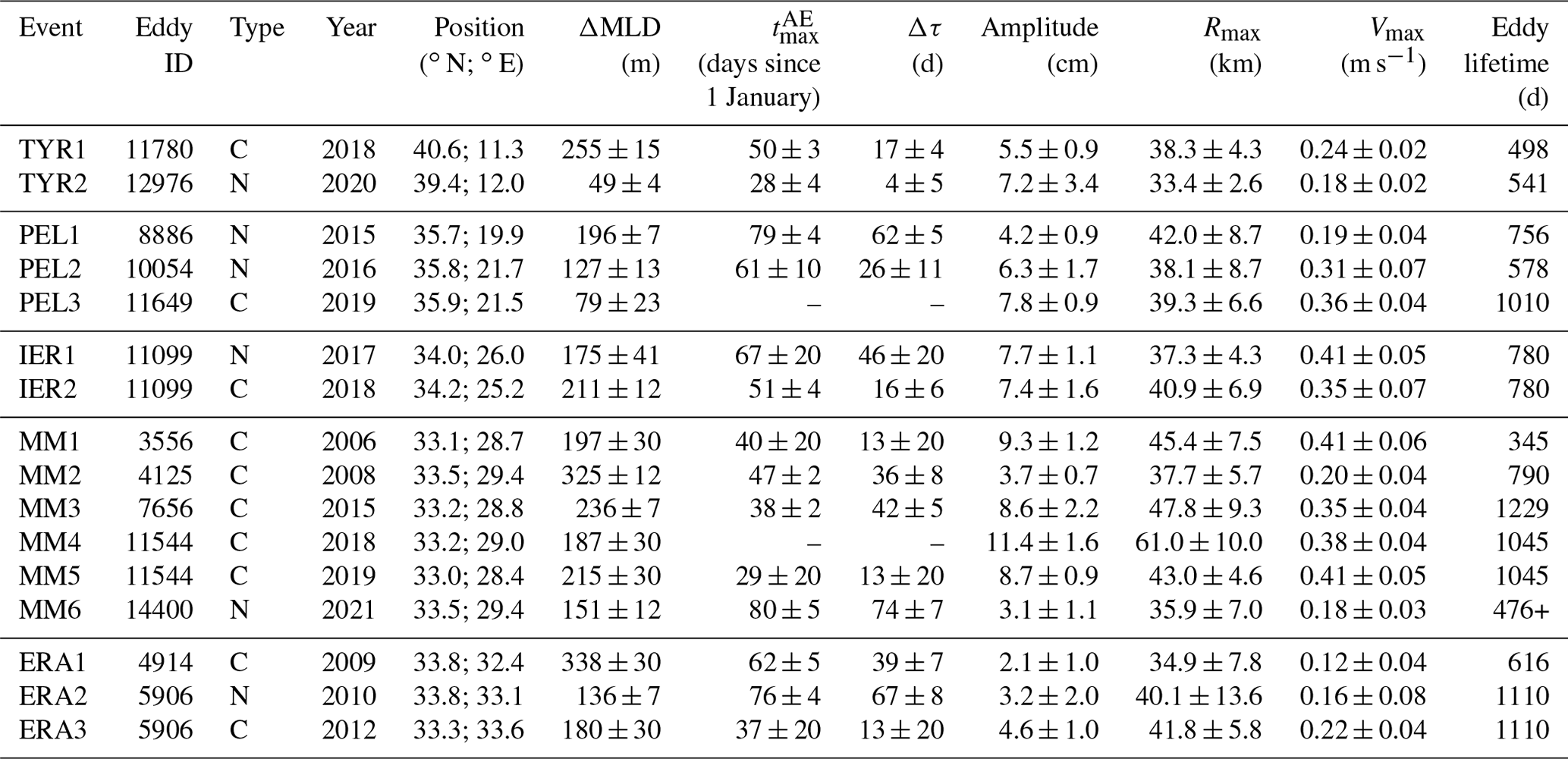
Table 1 Main characteristics of the 16 anticyclonic core mixed-layer deepening events studied; fitting method and uncertainties are detailed in Sect. 3.3. Eddy ID refers to track number in the DYNED-Atlas. Event types are “C” for “connecting” and “N” for “non-connecting”. Year “2018” corresponds to winter 2017–2018. Regions codes, ordered from west to east, stand for central Tyrrhenian (TYR), Pelops (PEL), Ierapetra (IER), Mersa Matruh (MM) and Eratosthenes (ERA). ΔMLD, $t_{\max }^{\mathrm{AE}}$ and Δτ are illustrated in Fig. 3. Note that sometimes two different winters are recorded in the same anticyclone (for example: “IER 1–2”) and that one eddy tracking (“MM 6”) stopped because the dataset finished in December 2021.

4.3 Inside-anticyclone MLD statistics

From 2000 to 2021, thanks to extensive Argo deployments sampling eddies, 16 winter MLD deepening events were accurately recorded with vertical profiles in 13 mesoscale eddies, 10 being “connecting” events and 6 being “non-connecting” ones. Several structures were surveyed over two winters (see Figs. 5 and 10). For each event, the fitting method detailed in Sect. 3.3 was applied, and parameters are reported in Table 1 together with eddy characteristics: eddy SSH amplitude, maximal speed V_max and maximal speed radius R_max. Eddy measurements are estimated by the mean from November to March of the corresponding winter. Figure 6 shows the location of each structure, which actually corresponds to types of long-lived structures already identified in the literature (Millot and Taupier-Letage, 2005; Hamad et al., 2006; Budillon et al., 2009; Barboni et al., 2021); these are listed from west to east as follows: Central Tyrrhenian anticyclone (abbreviated TYR), Pelops (PEL), Ierapetra (IER), Mersa Matruh (MM) and Eratosthenes (ERA). Position is computed as the mean position during the corresponding winter, even though eddies do not drift a lot in the Mediterranean Sea (Mkhinini et al., 2014). Despite regional differences and limited data availability, both types can occur in each region and provide an observation database allowing statistical comparison. Inside-eddy maximal MLD time $t_{\max }^{\mathrm{AE}}$ and hence Δτ could not be computed for events MM4 and PEL3, as gaps in the time series do not allow one to accurately measure them. However, ΔMLD could always be computed, as in worst cases there are still inside-eddy profiles later in the year, allowing one to check that maximal MLD was indeed reached (in a similar way to Moutin and Prieur, 2012, for previous winter MLD retrieved in April). Both types of events entail interaction (or lack thereof) with a deep subsurface homogeneous layer (layer with temperature gradient below $\mathrm{2.5}\times {\mathrm{10}}^{-\mathrm{3}}$ ^∘C m⁻¹ in absolute value), either a pre-existing one (see Figs. 4c, 5c and 10c) or a new one (see Figs. 5e and 10d). In all winter deepening events listed in Table 1, such homogeneous layers of least 50 m thick were indeed visible on vertical profiles. For Tyrrhenian Sea anticyclones (TYR1 and 2) with stronger salinity influence (Budillon et al., 2009), homogeneous layers with a density gradient below $\mathrm{5.0}\times {\mathrm{10}}^{-\mathrm{4}}$ kg m⁻⁴ were also visible. One can also notice that “non-connecting”' events are quite common, but double-core structures should be even more frequent. Indeed, a “connecting” event can occur inside a double-core structure and reconnect only the homogeneous core formed in the previous winter but not the deepest anomaly, as shown later in Fig. 10b–e. In other words, the proportion of “non-connecting” events in Table 1 and Fig. 6 should be considered as a lower bound for double-core structures, revealing their high occurrence.

Figure 7 Relationship between maximal MLD anomaly (ΔMLD) and eddy parameters possibly measured through remote sensing: (a) eddy SSH amplitude, compared with proposed 1 m MLD for 1 cm SSH relation (Gaube et al., 2019); (b) Rossby number (eddy intensity); and (c) Burger number (non-dimensional eddy size).

Hausmann et al. (2017) and Gaube et al. (2019) proposed a linear relation between the anticyclonic core MLD anomaly and its SSH amplitude, using regional average and monthly climatology. We previously showed that MLD anomaly varying over very short timescales can produce sharp MLD gradients and anomalies reaching several hundreds metres, which is not captured by smoothed composites. The relation between MLD anomaly and eddy amplitude is tested in Fig. 7a, distinguishing “connecting” (red dots) and “non-connecting” (green dots) events, together with the relation of Gaube et al. (2019) in the dashed line (1 m MLD anomaly for 1 cm eddy amplitude). This proposed relation is obviously not verified, the deep MLD observed in Mediterranean anticyclones exceeding by far the relation. On the opposite end, the deepest MLD anomalies seem to be observed in the eddies with the weakest SSH signature. Although surprising at first sight, this trend might be explained by the fact that the deepest MLD can be observed when the mixed layer abruptly connects to an anticyclonic deep homogeneous core in the subsurface, hidden by a strong seasonal thermocline. This is particularly the case for “ERA1” shown in Fig. 4, which has an extreme ΔMLD deeper than 300 m but the lowest SSH signature in Table 1.

The relation between the MLD anomaly and the eddy Rossby and Burger numbers is also tested in Fig. 7b and c. Rossby number, defined as $\mathit{\text{Ro}}=V_{\max }/f{R}_{\max }$, where f is the Coriolis frequency, is a non-dimensional measurement of the eddy intensity. The Burger number, defined as $\mathit{\text{Bu}}=(R_{\mathrm{d}}/R_{\max }{)}^{\mathrm{2}}$, with R_d being the deformation radius (8 to 12 km in the Mediterranean Sea), is a non-dimensional eddy size. Similarly to eddy SSH amplitude, no clear relation can be retrieved; deep and shallow MLD anomalies appear for various eddy intensities and sizes and for both “connecting” and “non-connecting” events. One can only notice that “connecting” events pull MLD deeper in general and that these events are slightly more observed in large structures (small Bu). Remote sensing measurements are then hard to link with observed eddy-induced MLD anomalies. On the opposite end, the diversity of vertical structures shown in this study (Figs. 4, 5 and 10) suggests that eddy vertical structure might have more influence, and previously proposed linear relations seem to apply mostly for surface-intensified structures.

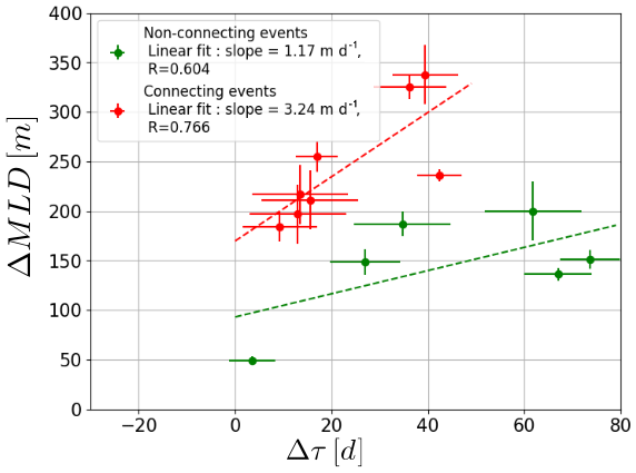
Figure 8 Scaling between the maximal MLD anomaly (ΔMLD) and restratification delay Δτ (see scheme in Fig. 3), distinguishing “connecting” (red) and “non-connecting” (green) events. Linear fit is applied separately, and correlation coefficient is put in the legend. Data and uncertainty are from Table 1.

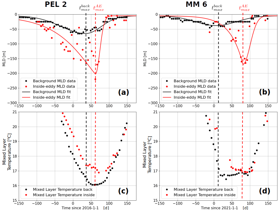
Figure 9 MLD data and fit for inside- and outside-eddy, illustrated for event PEL2 (a) and MM6 (b) (see Table 1). In the lower panel, corresponding mixed-layer temperature evolution for PEL2 (c) and MM6 (d) is shown. A dashed black (red) line marks the time of maximal background (inside-eddy) MLD.

4.4 Inside-anticyclone restratification delay

A new and important observation is that MLD inside anticyclones tends, on average, to clearly restratify later than the neighbouring background. It was shown for two individual events in Fig. 4 (ERA1, “connecting”) and Fig. 5 (ERA2, “non-connecting”), but it is statistically robust in Table 1: average $t_{\max }^{\mathrm{back}}$ is 22 d, and average $t_{\max }^{\mathrm{AE}}$ is 49 d, meaning restratification usually begins in the second half of February in anticyclones, on average 1 month later than outside-eddy. Restratification delay Δτ can reach 2 months in some cases: 67 d for ERA2 or 74 d for MM6 (see Fig. 9b). Figure 8a shows the relation between Δτ and ΔMLD and reveals that no clear trend can be identified alone: deep MLD anomalies are observed when the anticyclone MLD restratified early (low Δτ) or later (large Δτ). However, when distinguishing “connecting” and “non-connecting” events, a linear trend appears separately: MLD anomalies go deeper as Δτ increases, and for similar Δτ values, “connecting” events go deeper. Linear fit is performed separately for both types, shown by the dashed line in Fig. 8: for each day of continued MLD deepening inside anticyclones, a “connecting” (respectively “non-connecting”) MLD gets about 3 m deeper, with a correlation coefficient of 0.766 (1 m deeper, with a correlation coefficient of 0.604). This trend is logical, as a later restratification (large Δτ) lets the MLD deepen longer and hence leads to larger ΔMLD.

In order to analyse the MLD evolution together with the mixed-layer cooling, Fig. 9 shows in the upper panels the MLD fits (see Sect. 3.3) and in the lower panels the corresponding mixed-layer temperature for the PEL2 and MM6 events. Both events are representative of the observed evolution where the temperature can be followed over the whole winter. Maximal background MLD is reached for PEL2 (respectively MM6) around 30 January 2016 (10 January 2021), marking the end of background mixed-layer cooling with a plateau temperature of about 16 ^∘C, maintained for about 1.5 months (about 16.5 ^∘C for about 3 months) before warming up. In early 2016 (2021), the anticyclone core is indeed about +1 ^∘C warmer than its background, and it continues to cool for a while. The inside-eddy maximal MLD is reached around 1 March 2016 (20 March 2021) or +60 (+80) d in Fig. 9c (respectively Fig. 9d). A few weeks after, both background and anticyclonic core mixed layers started to warm again around 1 April (in both PEL2 and MM6), but background MLD started to restratify 1 month earlier in PEL2 (2 months earlier in MM6). Although it is hard to infer a mechanism from a few observations, it seems that the beginning of outside-eddy restratification does not mean that the mixed layer is warmed up again; rather, the outside-eddy mixed layer remains cold. The restratification delay seems to be the consequence of a maintained cooling of the initially warmer anticyclone core. Summer heating seems, on the other hand, to begin at the same time inside- and outside-eddy. Possible mechanisms driving this sustained mixing at the anticyclone core are discussed later in Sect. 5.3. An important observation is also that temperature difference between anticyclone core and the background is on the order of +1 ^∘C while MLD deepens but almost vanishes (or even becomes slightly negative) when the mixed layer warms again. Although sparse, these in situ observation are in total agreement with the observed eddy SSTA switch (Moschos et al., 2022) from winter warm-core anticyclones to predominant cold-core anticyclones with spring restratification in the Mediterranean Sea.

5 Discussion on physical drivers and perspectives

5.1 MLD anomaly scaling

We clearly identified the distinction between “connecting” and “non-connecting” events as a more important driver than other eddy parameters such as eddy amplitude, surface intensity or size (see Figs. 7–8), and this might explain the difficulty in finding a general law for any eddy-induced MLD anomaly. Indeed, “connecting” deepening mixed layers seem limited by the bottom of the pre-existing subsurface homogeneous core to which they connect (example in Fig. 4e), whereas “non-connecting” ones by definition do not go deep enough, are then expected to be limited by the heat loss, and are likely also influenced by the eddy. The other important parameter is the restratification delay (Δτ), measuring how long the anticyclone continues to deepen the MLD or not and which eventually scales with the maximal MLD anomaly. From a remote sensing perspective, both parameters seem very hard to assess without in situ profiles inside the eddies. Examples shown in this study (Figs. 4, 5 and 10 below) showed the complexity induced by possible connection with previous subsurface anomalies and, more generally, the key role of the anticyclone vertical structure that was totally smoothed in previous composite studies. The relationship between eddy-induced MLD anomalies and satellite measurements are definitely more complex. However, as theorized by Assassi et al. (2016), detecting remotely information on the eddy vertical structure could be possible, particularly distinguishing the subsurface- or surface-intensified nature by comparing eddy signatures in SSH and SST. For instance, the ERA1 event in Fig. 4 is an almost textbook case of a subsurface anticyclone with isopycnals doming, leading to a cold eddy SSTA.

5.2 Double-core eddy formation

The high occurrence of “non-connecting” events (crosses in Fig. 6) is very interesting, as they show the formation of double-core anticyclones through winter deepening of the surface layer above a pre-existing density anomaly. Double-core eddies were often surveyed in the world ocean (Lilly et al., 2003; Belkin et al., 2020), including in the western Mediterranean Sea (Garreau et al., 2018). Despite various propositions (see e.g. Belkin et al., 2020, for a list), no clear formation mechanisms emerged. Several studies focused on the so-called “vertical alignment” of two eddies with different densities in experimental works (Nof and Dewar, 1994), observations (Lilly et al., 2003) or modelling (Trodahl et al., 2020). Interestingly, Lilly et al. (2003) observed well in the Labrador Sea that double-core anticyclones mostly consist of convective lenses formed in different winters, the heat flux interannual variability leading to different density anomalies, but they explained double-core structures with eddies formed separately and that later aligned. There were nonetheless previous observations of the generation of a second lighter core above a pre-existing anticyclone. Thanks to repeated XBT transects, Nilsson and Cresswell (1980) surveyed such phenomena in an anticyclone detached from the East Australian Current, caused by winter heat loss. Bosse et al. (2019) surveyed this in the Lofoten Basin eddy with winter convection but through glider sections spaced in time and then with a temporal resolution on the order of a month. More recently, Meunier et al. (2018) explained the formation of a double-core Loop Current eddy by winter diabatic processes. However, this case is different from the Mediterranean anticyclones, as the Loop Current eddy consists of an advection of a large structure of Caribbean waters into the Gulf of Mexico, experiencing different surface fluxes with more heat loss and precipitation than the area where they originate. These diabatic processes by surface winter mixing result in a fresher, shallower core above a saline core of subtropical under-waters. Moreover, Meunier et al. (2018) explained quantitatively the observed anomaly against the regional average of atmospheric fluxes, whereas in our study, the differential MLD evolution between the eddy core and the background (Figs. 4a and 5a) suggested flux variations at the scale of the eddy.

What drives the formation of double-core structures should be further investigated, but one could expect the interannual variability of heat fluxes to be the main driver. This was already suspected by Lilly et al. (2003), although for them it was for separate eddies, and by Moutin and Prieur (2012). A winter with strong heat loss is expected to deepen MLD a lot, including inside-eddy, and a subsequently warmer winter would not be able to deepen the MLD as much. This mechanism drives mode-water formation, and it was already shown in other regions, mostly the Atlantic Ocean, that eddies could modulate mode-water formation (Dugan et al., 1982; Chen et al., 2022). Such a hypothesis could also explain the high occurrence of “non-connecting” events in the Mediterranean Sea, this region being known for a high interannual variability of winter heat loss. Pettenuzzo et al. (2010) found maximal winter heat loss to vary by 20 % to 30 % (in terms of regional monthly average) and also found a plausible connection with the North Atlantic Oscillation (NAO). This interannual variability of the heat flux was already shown to influence deep convection in the northwestern Mediterranean Sea (L’Hévéder et al., 2013); thus, a higher occurrence of double-core anticyclones due to a stronger Mediterranean Sea stratification in a warming climate could be expected (Somot et al., 2006).

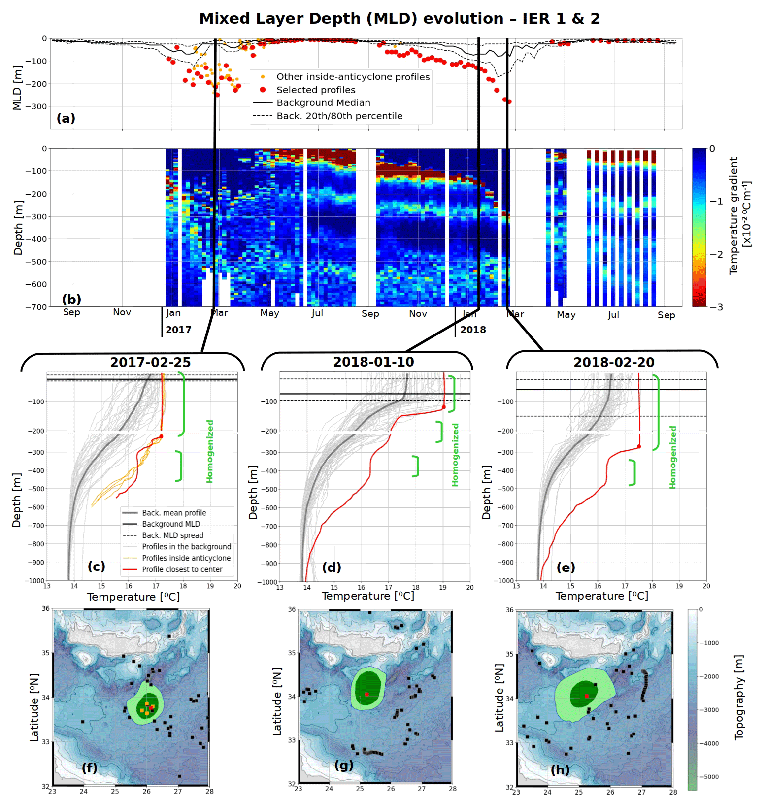
Figure 10 Same colour codes and legend as in Figs. 4 and 5 but for a Ierapetra anticyclone formed in 2016. Three vertical sections show respectively the mixing in early 2017 not reaching the deep subsurface core (c), the winter in early 2018 with a double core, the shallow core from winter 2017–2018 and the deep core still untouched (d), and at last the MLD deepening in March 2018 connecting the anomaly formed in March 2017 with the surface (e).

An important consequence in the formation of this lighter core in a “non-connecting” winter deepening is that the second core is separated from the surface by a thinner seasonal stratification. The next winter is then likely to connect again the new mixed layer with the upper core while possibly keeping the primitive deeper core untouched. Such an interaction from one winter to another was observed in the Ierapetra eddy and is presented in Fig. 10 (with the same colour code as in Figs. 4a–f and 5a–f). The Ierapetra eddy is a recurrent long-lived and intense anticyclone formed southeast of Crete (Theocharis et al., 1993; Lascaratos and Tsantilas, 1997; Ioannou et al., 2017) and recently surveyed by the PERLE 1 and 2 campaigns (Ioannou et al., 2019; Wimart-Rousseau, 2021). Similarly to Eratosthenes anticyclones previously shown, the density anomaly is mostly driven by a warm core, allowing the temperature profile to be used as a proxy for stratification (Ioannou et al., 2017). Figure 10 shows the Ierapetra anticyclone formed in autumn 2016. The first winter 2016–2017 turned out to be a “non-connecting” event (“IER1” in Table 1). Indeed, in March 2017, a pre-existing subsurface homogenized layer remained between 350 and 450 m, below the maximal anticyclonic core MLD of 220 m (Fig. 10c) and with about +2 ^∘C temperature anomaly. From April to December 2017, summer heating restratified the upper layer and left below a second homogeneous layer between ∼ 100 and 200 m deep. The primitive core remained homogenized at depth and was separated by a temperature gradient throughout the summer (Fig. 10b). In January 2018 (Fig. 10d), the inside-eddy vertical profile showed the mixed-layer deepening at 120 m, which was already deeper than the background MLD, and the double-core structure was still retrieved. At last, at the end of February 2018 (Fig. 10e), the MLD completely eroded the seasonal stratification and connected the current MLD with the previous winter's subsurface core, then reaching about 280 m. The winter 2017–2018 is then a “connecting” event (“IER2” in Table 1). The time series is interrupted inside the anticyclone, but Argo floats are again colocalized in May 2018, and despite some variability, a temperature gradient continuously separated the two cores between 200 and 250 m (see Fig. 10b). IER2 was then a “connecting” event on a double-core structure. The primitive anticyclonic core was not mixed but remained homogenized at depth. These data bring to light a possible formation process of a double-core anticyclone through winter convection and also document for the first time the fate of the formed subsurface anomaly, which can be tracked up to the next winter when it gets mixed again.

5.3 Physical drivers

The observed importance of restratification delay Δτ should also have underlying physical mechanisms. Prolonged MLD deepening and cooling inside-eddy (see examples in Fig. 9) leads to the extreme MLD anomalies sometimes larger than 300 m and hence to marked MLD gradients that occur at the scale of the eddy radius or shorter. Indeed, Gaube et al. (2019) found anomalies on the order of the mesoscale (R_m), but in a composite vision, and for large eddies compared to the deformation radius (small Burger numbers), MLD gradients in eddies should occur on shorter scales (Meunier et al., 2018). Such marked MLD gradients should trigger mixed-layer instabilities leading to restratification (Boccaletti et al., 2007; Fox-Kemper et al., 2008), which calls for mechanisms sustaining the mixing inside-eddy during the restratification delay. It should be noted that a homogenized layer itself does not prove active mixing but still reveals the absence of restratification. Interestingly, we also noticed that, in several cases, Argo floats remained well in the anticyclone core during the MLD deepening phase but often left the eddy soon after, which may be a signature for mixed-layer instabilities impacting the eddy. The first mechanism explaining longer mixing in anticyclones could be an eddy modulation of air–sea fluxes by eddy-induced SSTA. Villas Bôas et al. (2015) observed such eddy modulation on air–sea sensible and latent heat fluxes but in regions of energetic surface-intensified eddies with very warm anticyclones (particularly the Agulhas current retroflexion). For subsurface anticyclones, the eddy-induced SSTA is, on the opposite end, expected to be weakened (see the example of the cold-core anticyclone shown in Fig. 4e and the study of Assassi et al., 2016), and this mechanism might then not be the most important. MLD deepening enhanced in anticyclones could be explained by other eddy retroactions besides the heat fluxes, a possible mechanism being the eddy-induced Ekman pumping (Stern, 1965; Gaube et al., 2015) or enhanced mixing in anticyclones due to near-inertial wave trapping (Kunze, 1985).

5.4 Impact on eddy dynamics

Connecting events also raise interesting questions on the consequence of such mixing of deeper subsurface anticyclone cores, particularly the role of inside-eddy convection in relation to the eddy dynamics itself. Studies in the literature mostly focused on winter convection inside cyclones because of the preconditioning with isopycnals doming at their centre (Legg et al., 1998; Legg and McWilliams, 2001). Such a phenomenon should also applied to subsurface anticyclones due to the surface isopycnals doming and subsequent stratification weakening (Assassi et al., 2016). The coincidence of observed multiple “connecting” winters in long-lived anticyclones like the Mersa Matruh and Eratosthenes structures suggests a possible mechanism regenerating these structures, which maybe explains the extremely marked cyclone–anticyclone lifetime asymmetry in the Levantine Basin (Mkhinini et al., 2014; Barboni et al., 2021). Interestingly, Brenner (1993) already proposed winter cooling as a possible mechanism explaining the sustained lifetime of the anticyclone surveyed south of Cyprus. The other structure calling for comparison is the Lofoten eddy in the Sea of Norway and the Rockwall Trough eddy offshore Ireland, two long-lived deep anticyclonic structures. Winter convection was observed inside the core of the Lofoten eddy and was once thought to help regenerate the structure (Ivanov and Korablev, 1995; Köhl, 2007; Bosse et al., 2019). Double-core formation was also observed in the Lofoten eddy (Bosse et al., 2019). Recent numerical studies showed that this regeneration was primarily driven by the merging of smaller structures (Köhl, 2007; Trodahl et al., 2020); however, de Marez et al. (2021) showed that wintertime convection eased this merging process by deepening of the eddy core. Merging of eddies detached from the coast towards an offshore anticyclonic attractor was also observed in the Levantine Basin (Barboni et al., 2021), which could provide another explanation for the long-lived Mediterranean anticyclones. Cyclone–anticyclone asymmetry might not have just one mechanism, as other arguments have already proposed. Anticyclones indeed have a larger radius and are more coherent.

5.5 Biological impacts inside anticyclones

“Connecting”' the winter mixed layer in the Eratosthenes anticyclone was already observed by Krom et al. (1992) with a biogeochemical focus in 1989 (there called the “Cyprus eddy”). They measured a February inside-anticyclone MLD of 450 m (compared to 200 m) at the eddy boundary, with later spring restratification in May. Their temperature profile clearly corresponded to a “connecting” event, with even deeper MLD than in our study. Also comparing nitrates, phosphates and chlorophyll, they showed that chlorophyll production was about 30 % more abundant at the eddy core while being relatively similar to the Levantine Basin average at its edge. The main nitracline was consistently measured below the winter mixed layer and also at the eddy core, then around 450 m. While spring phytoplankton bloom occurred at the surface, they observed a mixed homogeneous layer that remained aphotic between the euphotic zone (the upper 120 m) and this deep main nitracline (called the “decomposition zone” in Krom et al., 1992). Here, they observed instead that, from February 1989 to January 1990, there was an increase in both nitrates and phosphates. Consequently, in the eddy, a second nitracline formed at the bottom of the euphotic layer at approximately the same level as a summer deep-chlorophyll maximum. Similarly, in another Eratosthenes structure in July 2008, Moutin and Prieur (2012) also estimated the maximal mixed layer in the previous winter to have reached 396 m and left only a stratified thermocline below, another clear description of a “connecting” winter mixing. Moutin and Prieur (2012) also observed in the eddy a main nitracline at roughly 400 m depth and a second one around 100 m together with a deep-chlorophyll maximum. The 100–400 m depth zone continued with low mineralization and high values of dissolved organic matter (DOC). From these observations, it seems that a “connecting” deep MLD induces a strong nutrient input to the euphotic layer but establishes in summer a homogenized aphotic subsurface layer with high DOC export at depth.

Neither of the two studies mentioned above observed the case of a “non-connecting” MLD, as frequently observed in our study and also in an Eratosthenes anticyclone (see Fig. 5). However, Moutin and Prieur (2012) discussed this possibility: if the winter MLD does not reach the main nitracline and/or phosphacline, it would keep the upper layer away from the deep nutriment source. The whole system would then evolve towards an ultra-oligotrophic system because of nutrients being very weakly injected to the euphotic layer. This is expected to be the case particularly when a primitive subsurface core does not connect to the surface for several winters, such as in the example of the Ierapetra anticyclone in Fig. 10. The high frequency of “non-connecting” anticyclone MLD observed in our study then suggests that anticyclones in the eastern Mediterranean Sea are to be considered ultra-oligotrophic systems more frequently than previously thought. Temporal evolution of such “non-connecting” events with biogeochemical instruments such as BGC-Argo would be interesting to follow this analysis.

6 Conclusions

In this paper, we were able to analyse, thanks to a combination of satellite observations and numerous in situ data, several time series that finely describe the evolution of the winter mixed layer in the core of Mediterranean anticyclones. We even succeeded in following, for the same long-lived anticyclone, the evolution of its MLD over 2 consecutive years. This allowed us to quantify extreme anomalies induced by mesoscale eddies in the mixed layer, which would have been smoothed in a standard composite analysis. Indeed, we observed that the winter mixed layer can go down to 380 m in the core of Levantine Basin anticyclones, while the surrounding background MLD does not go deeper than 80 m or 100 m.

We also observed a time lag of several weeks and sometimes of up to 2 months in the spring restratification between the core of these deep anticyclones and the background sea, revealing that MLD temporal evolution is not uniform. Indeed, when the later restratifies due to the rising temperature of the atmosphere, the core of these mesoscale anticyclones, which are warmer, continues to deepen and to cool. This time lag induces very strong spatial heterogeneities of the MLD in the eastern Mediterranean Sea during the early spring, with observed maximal MLD ranging from 50 to 330 m.

We showed that this localized deepening of the MLD is controlled by the vertical structure of these eddies. When the surface mixing layer connects with the subsurface core of pre-existing anticyclones, a rapid deepening of the surface mixed layer is observed. Conversely, when the surface mixed layer does not connect with the subsurface core, a double-core eddy is formed. Connection or not with pre-existing subsurface cores proves to be more relevant to a description of MLD deepening than other eddy parameters such as SSH amplitude or size. MLD anomalies were observed to linearly increase with restratification delay but increased roughly 2 to 3 times faster for “connecting” MLD than for the “non-connecting” one.

These extreme MLD deepenings in anticyclone cores reveal complex and rich interaction between the surface and subsurface of the eddies. Connection between the mixed layer and subsurface anomalies provides a way to propagate heat at depth while mixing in winter, the consequences of which remain to be investigated. These winter deepenings inside anticyclones could also play a role in sustaining the extremely long-lived anticyclone in the eastern Mediterranean. MLD anomalies in cyclonic eddies remain to be investigated, and an open question would be to know if a restratification delay could also be observed in cyclones.

Appendix A: In situ profile-checking methodology

In both CORA-DT (Szekely et al., 2019b) and Copernicus-NRT (Copernicus, 2021) datasets, vertical profiles data coming from XBT, CTD, glider and profiling floats are collected by selecting files with respective data type codes XB, CT, GL and PF. When a profile from 2000 to 2019 was available in both DT and NRT mode, it was retrieved from the CORA-DT dataset, which performs more quality checks (Szekely et al., 2019a). Selection was done with the following steps, separately for temperature and salinity, and when available, “ADJUSTED” properties were collected:

• Position and date quality control (QC) flags equal to 1, 2 or 5 and position not on land.

• Select the first valid value (QC = 1,2 or 5) above 50 m, the last valid value below 400 m, and at least 40 measurements between 50 and 400 m.

• Temperature data below 12 ^∘C or above 35 ^∘C are discarded, and salinity data below 30 PSU or above 42 PSU are discarded. These parameters are specific to the Mediterranean Sea.

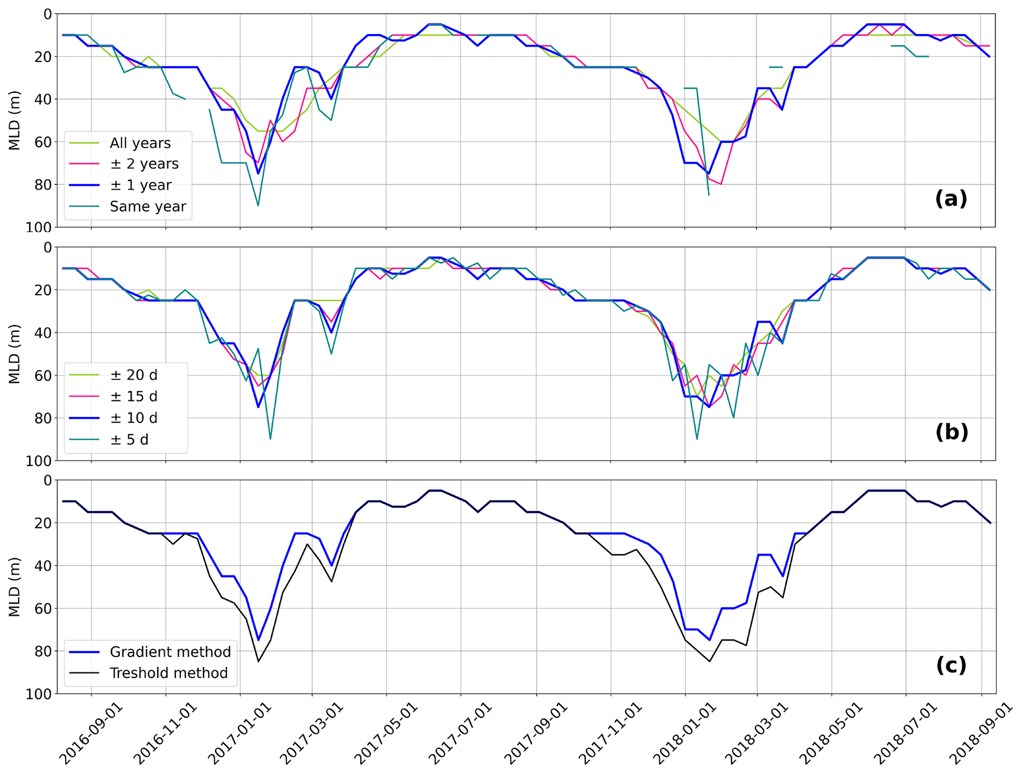
Figure A1 Sensitivity of the background MLD on the different parameters for events IER1–2 (see Table 1 and Fig. 10a): (a) Δy (year interval) and (b) Δday (day interval). (c) Sensitivity to the MLD computation method. The background MLD method used throughout this study is Δday =10 d, Δy =1 year and the gradient method (common navy blue line on panels a–c).

• When both temperature and salinity are available, density is computed using the TEOS-10 equation (McDougall et al., 2013) from the Python package gsw (https://teos-10.github.io/GSW-Python/, last access: 21 February 2023).

• Profiles are linearly interpolated on the same vertical grid, with 5 m grid steps from 5 to 300 m depth and 10 m grid steps from 300 to 2000 m. The maximal gap allowed is 20 m, and profiles with gaps are discarded.

• Profiles with temperature jumps higher than +6 ^∘C or −2 ^∘C (positive upwards) between two grid points are discarded, as they are assumed to be unrealistic. This is required particularly to filter out noisy XBT profiles.

• After these steps, only profiles with more than 40 data on the interpolated grid between 50 and 400 m are kept.