Modeling the interannual variability in Maipo and Rapel river plumes off central Chile

River plumes have a direct influence on coastal environments, impacting coastal planktonic and benthic communities, including fishery resources. In general, the main drivers of river plume dynamics are the river discharge and the alongshore wind stress, whereas the tides and topography play a secondary role. In central Chile, rivers flowing into the eastern Pacific have a relatively short path on land, with a high slope and a mixed snow–rain regime. This study aims to understand the interannual variability in the plumes of the Maipo and Rapel rivers in the coastal/shelf area off central Chile and their influence on local ocean dynamics. We used the Coastal and Regional Ocean Community (CROCO) model, with 1 km horizontal resolution and 20 sigma levels, to simulate the ocean dynamics for the period 2003–2011. The results show that the plume's area coverage and coastal ocean salinity are strongly correlated with the river discharges. The predominant northeastward winds control the plumes' orientation toward the northwest. However, episodes of southeastward winds in winter can reverse the plumes' direction, promoting their attachment to the coast and southward transport. Results also show a salification trend linked to the severe droughts hitting central Chile during the studied period. This salification determines a change in local dynamics which could be more frequent in future scenarios of climate change with a significant lack of rain and river discharges along central Chile.

1 Introduction

Among coastal ecosystems, river plumes are relevant marine areas because of their impact on physical and biogeochemical processes driving the seasonal and spatial dynamics of planktonic communities (D'sa and Miller, 2003; Mestres et al., 2003; Masotti et al., 2018). The most evident characteristics of river plumes are their low salinity, strong stratification, the generation of buoyancy-driven currents around the frontal area and the higher turbidity associated with suspended solids. Although there are many forcings influencing the dispersion and dynamics of river plumes (e.g., tides, topography, inertia, local circulation, Earth rotation and buoyancy), river discharge and wind stress dominate river plume dynamics (Fong and Rockwell Geyer, 2001; Lentz and Largier, 2006; Fernández-Nóvoa et al., 2015; Horner-Devine et al., 2015). For instance, Hetland (2010) demonstrated that the magnitude and length scale of cross-shore plume density changes are directly proportional to the river discharge. On the other hand, a recent study demonstrates that infra-gravity wave forcing has considerable influence on the near-field plume dynamics (Flores et al., 2022), which could influence mixing and cross-shore dispersion.

A proper description of the variability in and trend of variables like salinity, nutrients and suspended solids in river plumes allows us to estimate the condition of the catchment–coast system, where activities like deforestation, agriculture and urban inputs can change the temporal pattern and influence of river discharges (Acker et al., 2009; Bainbridge et al., 2012; Martínez et al., 2018, 2022), in addition to the effects associated with climate change. For instance, by comparing different river systems, Acker et al. (2009) concluded that a decreasing trend in chlorophyll concentration within the river-influenced area is associated with a reduction in the river discharges.

River plumes usually have high nutrient content and support primary production and algal biomass (Mallin et al., 2005; Peterson and Peterson, 2008; Kudela and Peterson, 2009). The influence of river plumes on larval transport and survival is related to their tolerance of osmotic shocks and their capacity to move vertically through the water column and density gradients (Bloodsworth et al., 2015). Different taxonomic groups will have different conditions to move and survive within river-influenced environments (Bloodsworth et al., 2015). Similarly, the influence of the river plume on sediments and benthos can be observed several kilometers (Forrest et al., 2007) to hundreds of kilometers (Grimes and Kingsford, 1996) from the river mouth. Other studies have demonstrated that the turbidity associated with the plume can influence the predation mortality of larval fish (Carreon-Martinez et al., 2014) and phytoplanktonic communities (Chakraborty and Lohrenz, 2015). The reduction in river discharges can have a negative impact on fishery resources, biodiversity and ecological functions (Fan et al., 2022). For instance, Vargas et al. (2006) described the influence of the Maipo River plume, central Chile, on the distribution of chlorophyll and barnacle larvae on the inner shelf.

Several studies have demonstrated the importance of wind forcing in river plume dynamics by combining numerical modeling results with remote sensing and in situ observations. Choi and Wilkin (2007) demonstrated the strong influence of buoyancy and wind forcing on the Hudson River plume. Similar findings were described for the Yukon River plume by Clark and Mannino (2022). The change in the river plume direction caused by winds associated with the passage of low-atmospheric-pressure systems was investigated using the Navy Coastal Ocean Model (Cobb et al., 2008). The plume extension and orientation driven by the river discharge–wind interplay were described by Dong et al. (2004) for the Pearl River plume. An interesting modeling study showed the influence of the Columbia River plume on the continental shelf during upwelling conditions, affecting the alongshore and cross-shore momentum transport as well as the vertical turbulence structure (Fulton, 2007). Normally, the river plume flows northward along the Washington coast, but in spring–summer the upwelling-favorable winds and coastal circulation force the plume farther south and offshore off Oregon (Hickey et al., 2005; Saldías et al., 2016). In general, the role of the wind forcing is enhanced for small river plumes (Osadchiev et al., 2021; Basdurak and Largier, 2022), which is the case for most river outflows along central-southern Chile (Saldías et al., 2016).

The relevance of combining hydrodynamic models with remote sensing and in situ data has been highlighted by Devlin et al. (2015), who studied the river plumes on the Great Barrier Reef using MODIS imagery. In another study, Bai et al. (2010) used MERIS sensor data to characterize the Changjiang Estuary. In a recent study, Bainbridge et al. (2012) used MODIS images to describe the influence of river discharge, wind and Coriolis forcing on the Burdekin River plume and the transport of fine sediments and nutrients. In a study focused on the Amur River, Abrosimova et al. (2009) compared direct observations with MODIS images and concluded that the plume is highly dynamic and is mostly controlled by the Earth's rotation in comparison with the plume inertial effects.

Central Chile is a region characterized by the presence of several rivers that discharge freshwater and sediment mostly in winter; this region exhibits almost permanent upwelling-favorable southwesterly winds and the presence of Subantarctic Water (SAAW), sometimes with remnants of Subtropical Water (STW), with salinities higher than 34.4. Recent studies of river plumes off central Chile have been conducted using satellite imagery (Saldías et al., 2012, 2016) and numerical modeling results (Salcedo-Castro et al., 2020; Rojas et al., 2023; Vergara et al., 2023). These studies described river plumes with sea surface salinity (SSS) values typically lower than 33.9 (Piñones et al., 2005; Saldías et al., 2012; Salcedo-Castro et al., 2020; Vergara et al., 2023) and a high seasonality in plume spreading and turbidity signals associated with the river discharges. In austral winter, a larger areal extent and the merging of the plumes can be observed after storms (coalescence events), whereas smaller plumes restricted to the near-field region are observed in austral spring–summer. A recent study combining remote sensing and numerical modeling results confirms that the river plumes and flow field are primarily modulated by the wind forcing in winter (Rojas et al., 2023). This work also highlights that the geostrophic component of the flow is associated with the wind modulation of the plume's shape on a synoptic scale.

This study aims to describe the interannual variability in the circulation and hydrographic conditions (and stratification) in the coastal area influenced by two rivers off central Chile: the Maipo and Rapel rivers, complementing a previous study by Salcedo-Castro et al. (2020) which was focused on the plume-spreading climatology and vertical structure. To the best of our knowledge, this is the first interannual modeling study of these river plumes.

2 Methods

2.1 Study area

The study area, delimited by 32^∘30^′–34^∘ S latitude, is representative of the Mediterranean climate of central Chile, where the Maipo and Rapel rivers are discharged (Fig. 1). These are mixed rivers with snow- and rain-fed regimes, having higher discharges in winter and late spring. Like most Chilean rivers, they cover a relatively short distance across transverse and longitudinal valleys between the mountains and the coast and have a small watershed (Saldías et al., 2012). However, their discharges are altered by activities associated with mining, agriculture, industries and urban development, as there are several cities with large populations along the rivers. The lower part of the Rapel River is downstream of Rapel Dam, a reservoir finished in 1968. In the lower coastal–estuarine region, the river discharges are under the influence of tides and local topography, characterized by a partially opened sandbar, with a strong seasonal wind influence (Flores et al., 2022).

Figure 1 Study area showing the Maipo and Rapel rivers. The dashed red line represents the transect to describe the temporal variation in sea surface salinity (SSS) and vertical structure across the study area (see Figs. 10 and 12).

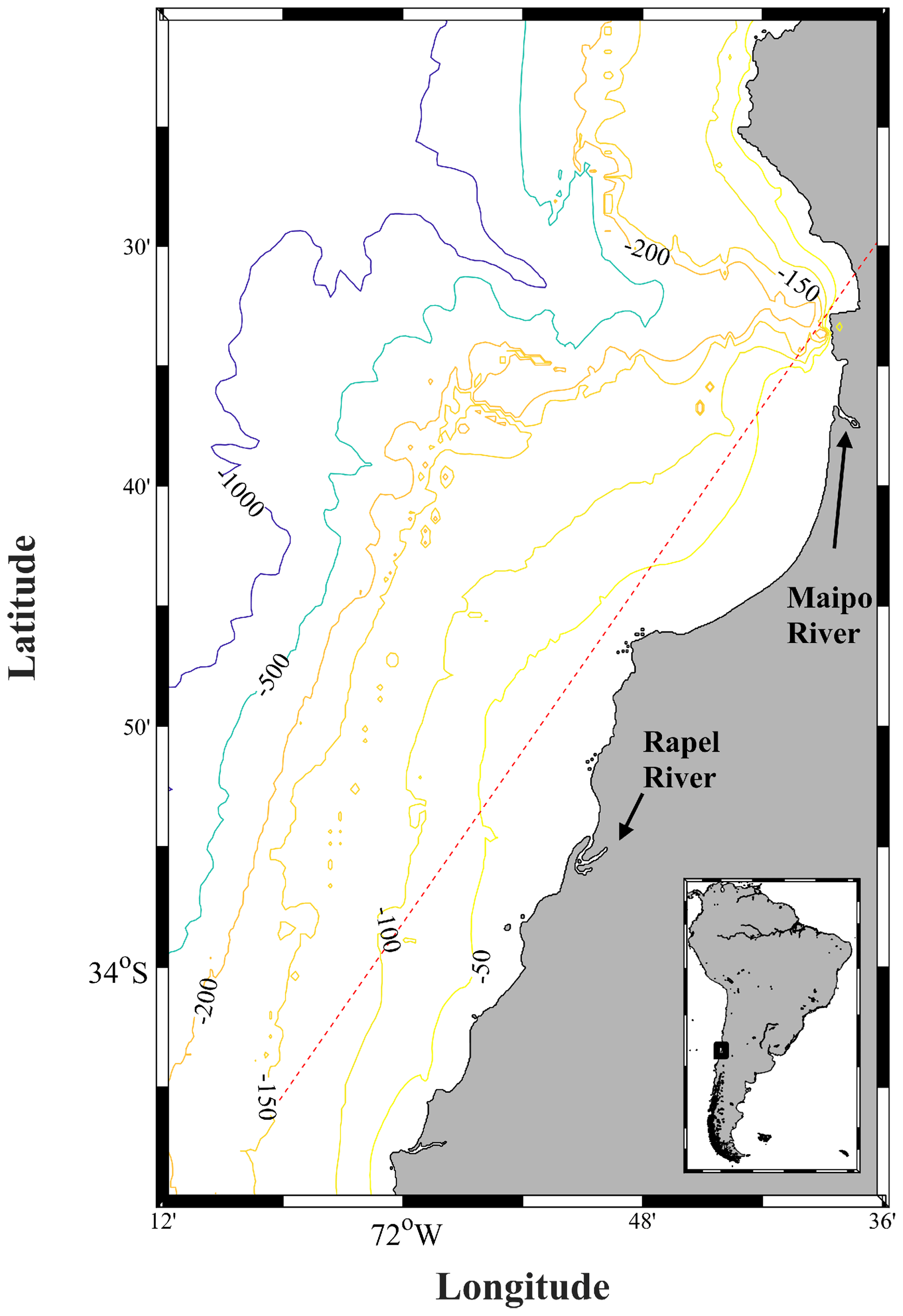
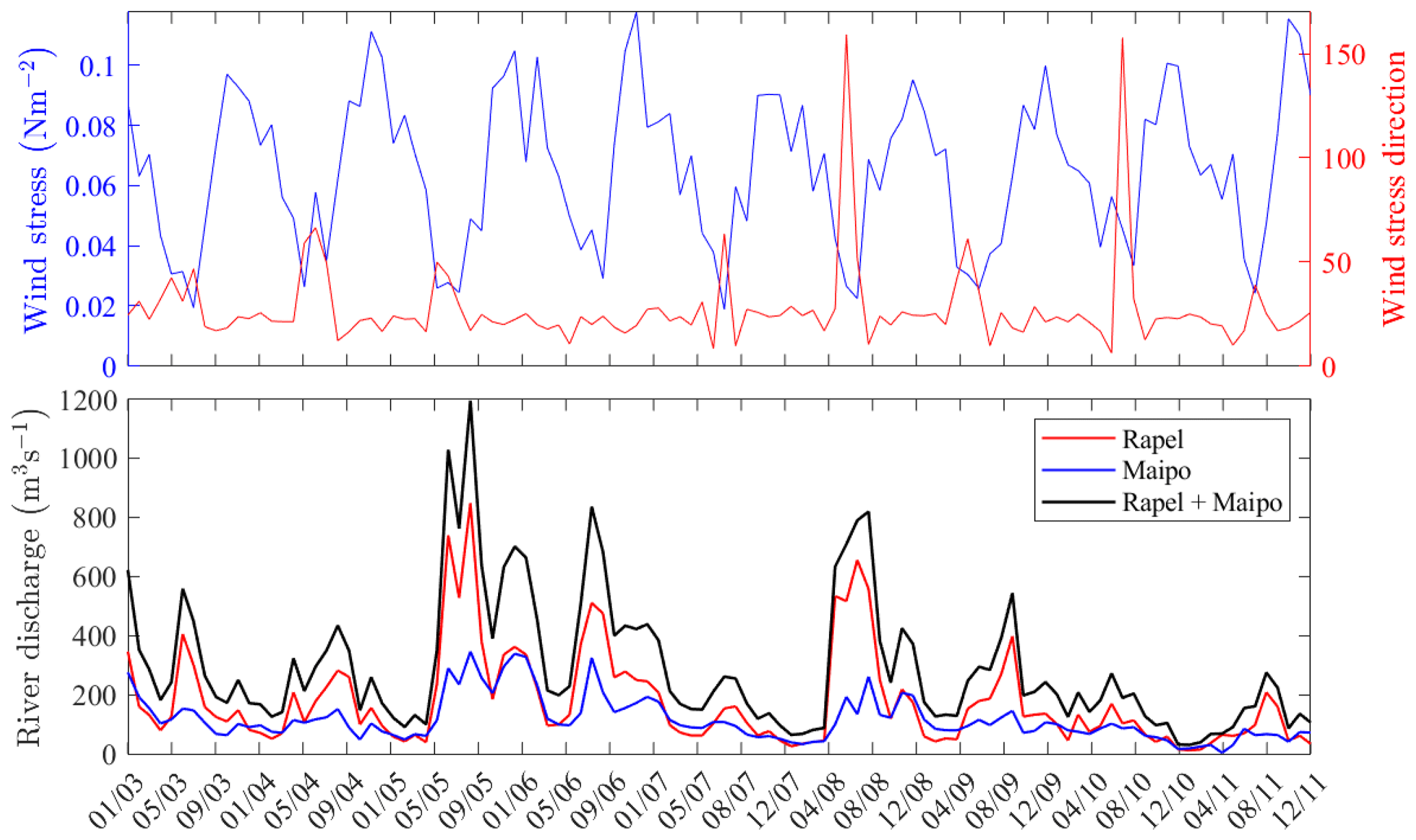
Figure 2 Monthly mean wind stress (OFES NCEP) and river discharges (monthly averages) used to force the model in the study area.

2.2 Numerical model

We used the Coastal and Regional Ocean Community (CROCO) model and CROCO_TOOLS package (http://www.croco-ocean.org, last access: 29 February 2021). This version solves the primitive hydrostatic equations of ocean dynamics; uses the terrain-following coordinate; and is an adaptation of ROMS_AGRIF (Penven et al., 2006; Debreu et al., 2012), which is based on a new nonhydrostatic and a non-Boussinesq solver developed within the former ROMS kernel (Shchepetkin and McWilliams, 2005), for optimal accuracy and cost efficiency (Hilt et al., 2020). The model was configured with a 1 km horizontal resolution (Arakawa C grid) and 20 vertical levels, with higher resolution toward the surface and bottom levels. This configuration allows us to resolve sub-mesoscale features of the river plumes and their interaction with mesoscale processes. The model momentum and buoyancy fluxes were forced with the Scatterometer Climatology of Ocean Winds (SCOW; https://chapman.ceoas.oregonstate.edu/scow/, last access: 29 February 2022) and the Comprehensive Ocean-Atmosphere Data Set (COADS; https://iridl.ldeo.columbia.edu/SOURCES/.COADS/, last access: 29 February 2022), which have a 25 km resolution. Boundary conditions were obtained from the 10 km resolution Ocean General Circulation Model for the Earth Simulator (OFES), which was forced with fluxes from the National Centers for Environmental Prediction (NCEP). Daily river discharges from the Maipo and Rapel rivers were obtained from the General Water Department (Dirección General de Aguas, Chile) and complemented with the CAMELS-CL dataset (Alvarez-Garreton et al., 2018). The Rapel River gauge is located 25 km downstream of the dam and 16.5 km from the river mouth. The Maipo River gauge (Cabimbao Station) is 21 km upstream of the river mouth. The monthly mean wind forcing and river discharges in the study area are shown in Fig. 2. The modeled period was 2003–2011, which is probably not quite enough to reflect the effect of long-term climatic events like the Pacific Decadal Oscillation (PDO); however, our simulations encompassed contrasting years with El Niño and La Niña affecting the river discharges and the plumes in the coastal ocean.

The horizontal distribution of salinity was described to study the spatial–temporal variability in the plumes. A salinity value of 33.8 was used to delimit the plumes from ambient waters after computing monthly averages; this value is consistent with the reference value described by Rojas et al. (2023). To estimate the plume's area, a finer grid was generated by linear interpolation and then exported as GeoTIFF images. These images were processed on ArcGIS Pro to measure the plume area and mean plume sea surface salinity (SSS).

Along with the description of salinity distribution, we also estimated the horizontal gradient of salinity (Yu, 2015; Freeman and Lovenduski, 2016; Saldías and Lara, 2020; Bao et al., 2021) as an indication of the strength of the plume's frontal characteristics. We computed the meridional (Sgrad_(x)) and zonal (Sgrad_(y)) gradients according to Eqs. (1) and (2), respectively, which were combined to obtain the gradient magnitude at the center of each 1 km² grid cell (Sgrad) (Eq. 3).

$$\begin{array}{}\text{(1)}& {\displaystyle }\begin{array}{rl}& {\mathrm{Sgrad}}_{\left(x\right)}=\\ & {\displaystyle \frac{\mathrm{1}}{\mathrm{2}}}\left({\displaystyle \frac{S_{(i+\mathrm{1},j)}-S_{(i,j)}}{{\mathrm{Long}}_{(i+\mathrm{1},j)}-{\mathrm{Long}}_{(i,j)}}}+{\displaystyle \frac{S_{(i+\mathrm{1},j+\mathrm{1})}-S_{(i,j+\mathrm{1})}}{{\mathrm{Long}}_{(i+\mathrm{1},j+\mathrm{1})}-{\mathrm{Long}}_{(i,j+\mathrm{1})}}}\right)\end{array}\text{(2)}& {\displaystyle }\begin{array}{rl}& {\mathrm{Sgrad}}_{\left(y\right)}=\\ & {\displaystyle \frac{\mathrm{1}}{\mathrm{2}}}\left({\displaystyle \frac{S_{(i,j+\mathrm{1})}-S_{(i,j)}}{{\mathrm{Lat}}_{(i,j+\mathrm{1})}-{\mathrm{Lat}}_{(i,j)}}}+{\displaystyle \frac{S_{(i+\mathrm{1},j+\mathrm{1})}-S_{(i+\mathrm{1},j)}}{{\mathrm{Lat}}_{(i+\mathrm{1},j+\mathrm{1})}-{\mathrm{Lat}}_{(i,j)}}}\right)\end{array}\text{(3)}& {\displaystyle }\mathrm{Sgrad}=\sqrt{{\mathrm{Sgrad}}_{\left(x\right)}^{\mathrm{2}}+{\mathrm{Sgrad}}_{\left(y\right)}^{\mathrm{2}}}\end{array}$$

We used Eq. (4) to compute the area-averaged salinity gradient (AASG) in the whole domain (Salcedo-Castro et al., 2015), where “area” is the surface of each 1 km² grid cell and “total area” is the model's total domain surface.

$$\begin{array}{}\text{(4)}& \mathrm{AASG}={\displaystyle \frac{\mathrm{1}}{\mathrm{total}\mathrm{area}}}\sum _{i=\mathrm{1},j=\mathrm{1}}^{i=m,j=n}{\mathrm{Sgrad}}_{i,j}\times {\mathrm{area}}_{i,j}\end{array}$$

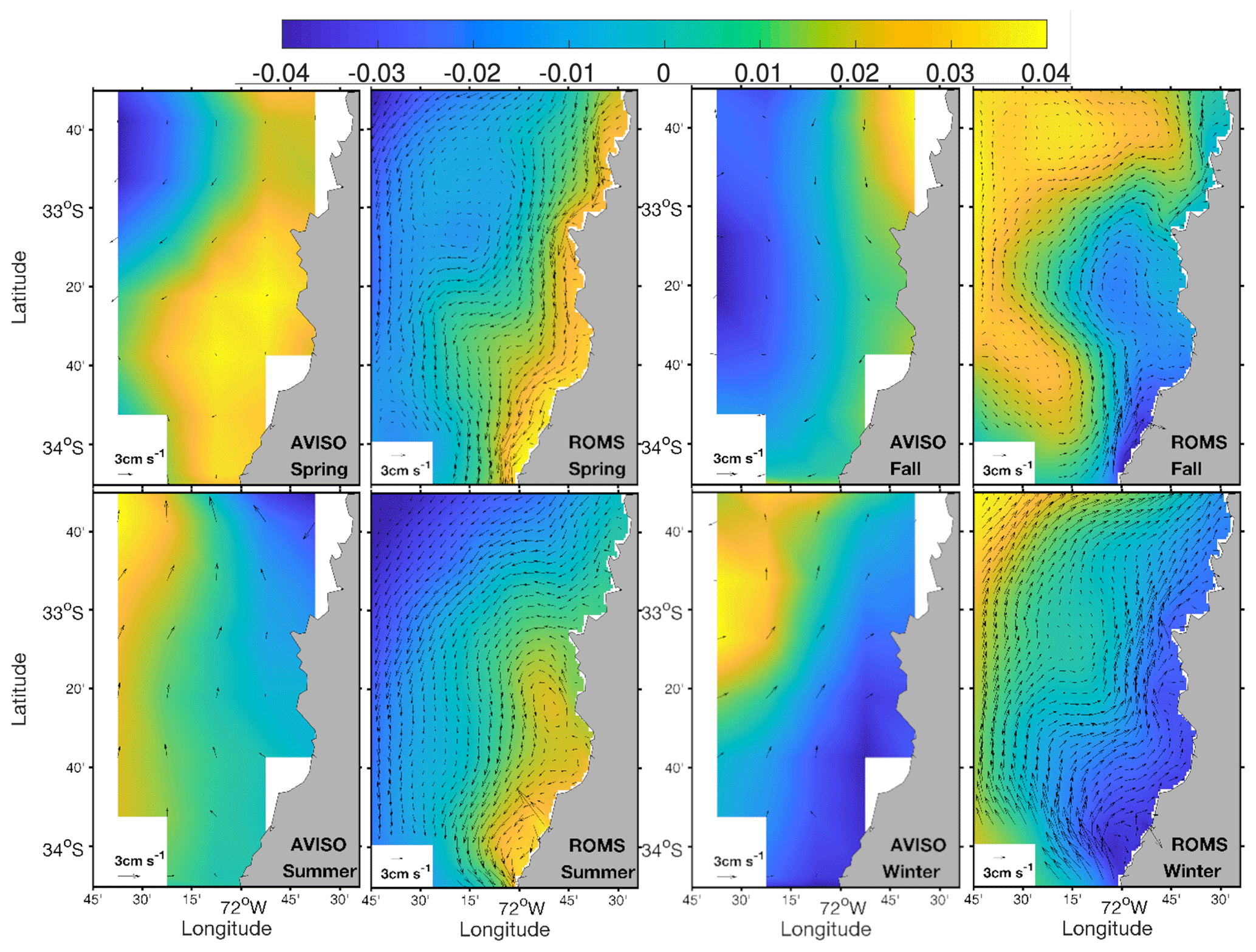
Figure 3 Comparison of mean seasonal sea surface height anomaly (SSHA) (m) and geostrophic currents from AVISO and the CROCO model.

The stratification in terms of the contribution by river discharges was assessed through the potential energy anomaly (PEA, J m⁻³) (Simpson et al., 1978; O'Donnell, 2010; Rojas et al., 2023) (Eq. 5):

$$\begin{array}{}\text{(5)}& \mathit{\varphi }={\int }_{-H}^{\mathit{\eta }}g(\mathit{\rho }-\stackrel{\mathrm{‾}}{\mathit{\rho }})z\mathrm{d}z.\end{array}$$

Here ϕ is the potential energy anomaly, g is the gravity acceleration, ρ is the local density at depth z, and the term $\stackrel{\mathrm{‾}}{\mathit{\rho }}$ corresponds to the depth-averaged density (Eq. 6):

$$\begin{array}{}\text{(6)}& \stackrel{\mathrm{‾}}{\mathit{\rho }}={\displaystyle \frac{\mathrm{1}}{H}}{\int }_{-H}^{\mathit{\eta }}\mathit{\rho }\left(z\right)\mathrm{d}z,\end{array}$$

where H is the total depth and η is the free surface.

We evaluated the PEA between 1 and 20 m along the transect depicted in Fig. 1 to represent the strength of stratification, as this represents the equivalent work to homogenize the water column (Simpson, 1981).

2.3 Empirical orthogonal functions (EOFs) and wavelet analysis

We performed an empirical orthogonal function (EOF) analysis (Emery and Thomson, 2004) of the daily model outputs to evaluate the interannual variability in the plumes, reducing the dimensions of large datasets to a few significant orthogonal (uncorrelated) modes of variability and their associated time series (represented by the principal components, PCs). Considering that geophysical time series can be hard to interpret because of the presence, even in the first modes, of complex non-periodic signals (e.g., Olita et al., 2011a), we analyzed the spectrum of the PCs by means of the continuous wavelet transform (CWT). The CWT allows the localization of a signal in the time domain while neglecting some localization in frequency (Torrence and Compo, 1998). The rectification of the wavelet power spectra was calculated following Liu et al. (1998). We used the Morlet wavelet after removing the trends. Thus, spurious low-frequency signals are not considered in the analysis. The trend identification was performed by least-squares linear fit. The main variable for this analysis was the sea surface salinity, considering our focus on river plumes that incidentally have a strong signal in salinity. We also analyzed surface currents, in order to investigate where these currents could be influenced by surface plumes, or vice versa. This was done by considering separately meridional and zonal components of the flow.

3 Results

3.1 Horizontal plume pattern

Prior to analyzing the horizontal plume pattern, a qualitative validation of the model was carried out. Considering the unavailability of direct observations (mooring), we used altimetry data from AVISO (Archiving, Validation and Interpretation of Satellite Oceanographic data, http://www.aviso.altimetry.fr, last access: 6 October 2023) to estimate geostrophic currents and compare them with those computed from the model, following Aguirre et al. (2012). As shown in Fig. 3, the mean seasonal geostrophic currents compare well between the model and AVISO, considering the differences in the spatial resolution and the problems normally associated with the satellite sensor close to the coast and the smoothing caused by gridding fields from multiple altimeters (Aguirre et al., 2012). The strong contrast observed in summer is probably associated with the coastal upwelling and varying interannual forcing during the study period (Aguirre et al., 2012). Moreover, this difference is not relevant as the plume dynamics mostly occur during winter–spring. Additionally, we evaluated the model's performance by means of the reflectance associated with suspended sediment, given that the sea surface salinity (SSS) is tightly correlated with this variable in river plume regions. According to previous studies (Saldías et al., 2012, 2016; Masotti et al., 2018), total suspended solids are better sensed in the 645 nm band; therefore, we worked with the same band. We computed the 99th percentile (P99) of the 645 nm reflectance in the model domain to compare it with the total river plume area and SSS. Firstly, we tested the validity and consistency of MODIS imagery by comparing the 99th percentile of the 645 nm reflectance in the model domain against the river's discharge, obtaining r² = 0.76. Similarly, when comparing the monthly plume area and mean SSS within the plumes versus MODIS (P99), the correlation was r² = 0.56 and r² = 0.46, respectively.

The sea surface salinity (SSS), averaged over the 9-year period, and its standard deviation (SD) are shown in Fig. 4. The plumes are restricted to a relatively small area next to the river mouths and mostly oriented in the NW–NNW direction. This also reflects the mean direction of surface currents driven by northeastward winds. The SD field reflects the largest variability associated with the lowest mean salinity near the river mouths – the plume's signal responds to the pulses of river discharges.

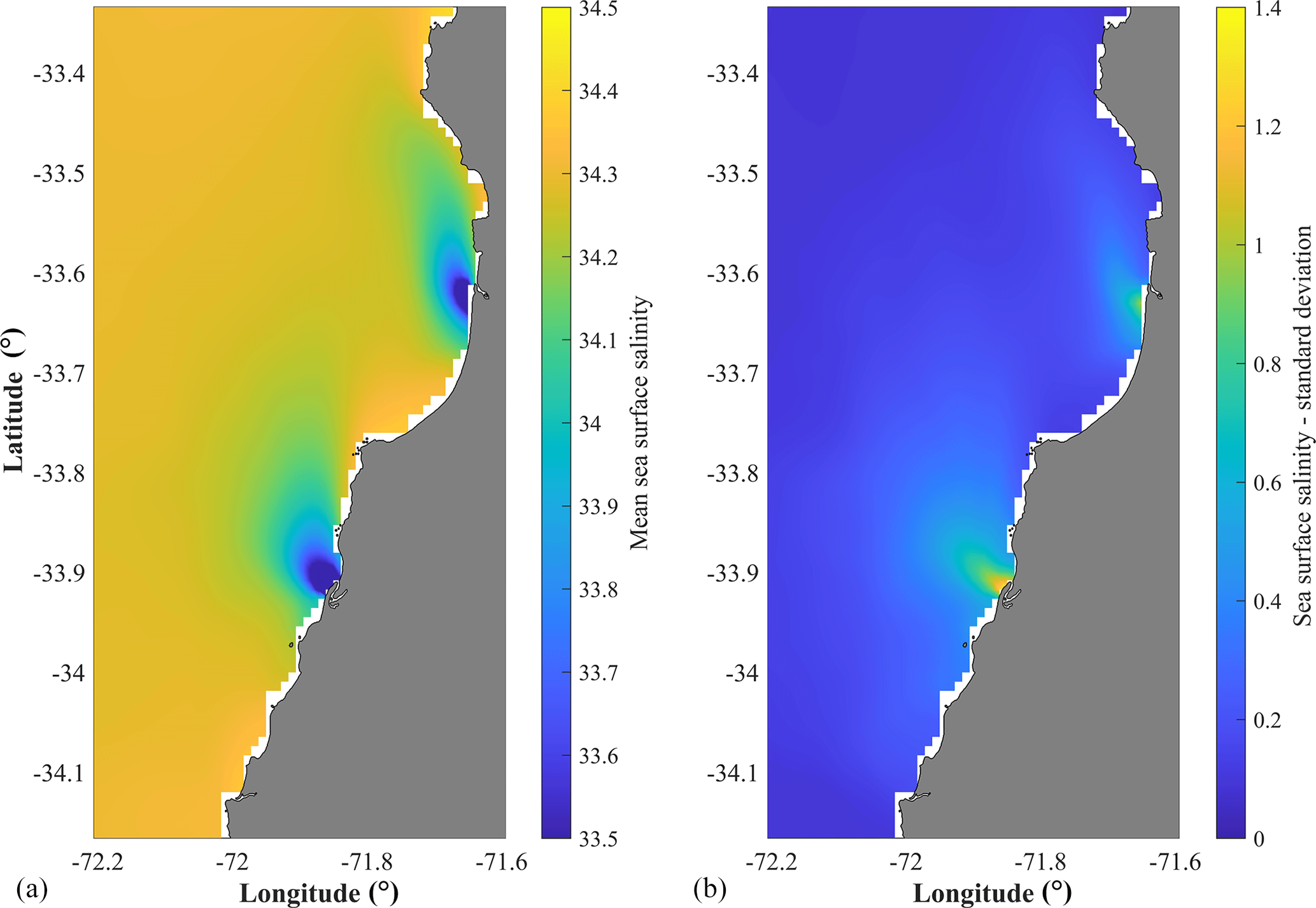
Figure 4 Maps of (a) averaged sea surface salinity and (b) sea surface salinity standard deviation over the 9-year period.

The strong dependence of the plume horizontal pattern on the wind direction is especially evidenced during some winter months (Fig. 5), when wind is able to reverse the plume's northwestward direction. This is the situation observed in June 2008 and July 2010, corresponding to the two largest peaks observed in the wind stress direction shown in Fig. 2. The plumes presented contrasting spreading in the coastal ocean in response to the wind forcing; in winter 2008, the mean wind stress was 0.05 N m⁻², whereas the wind stress was predominantly 0.07 N m⁻² in July 2010.

We defined the limit of the plume's area with a salinity value of 33.8 in order to separate the plumes from ambient waters. A practical reason for choosing 33.8 as a limit was that the plumes kept a maximum regular shape within the domain when using this value. However, the main reason to define the 33.8 threshold is that this is a typical value to identify the Subantarctic Water (salinity: 33.8–33.9), the characteristic surface water mass in this region. Consequently, the rationale is that all waters fresher than that salinity must be from the plumes and not from a regional water mass. In a similar approach, this limit coincided with the values defined by other authors that have studied river plumes in Chile (Saldías et al., 2012; Flores et al., 2022). Other authors have applied other criteria, depending on the objectives of the study and the dynamic characteristics of the area under study (Falcieri et al., 2014). The variation in the plume area (< 33.8), total river discharge (Maipo + Rapel) and mean plume surface salinity is shown in Fig. 6. It is possible to see a direct correlation between the total river discharge and the plume area (Fig. 7a) and an inverse correlation between the total river discharge and the mean plume surface salinity (Fig. 7b).

The minimum and maximum salinity in the domain shows a clear increasing salinity trend over the entire period (Fig. 8), which is related to a gradual decrease in river discharge. The interannual variability revealed major plume events with reduced salinity during the winters of 2005 and 2008.

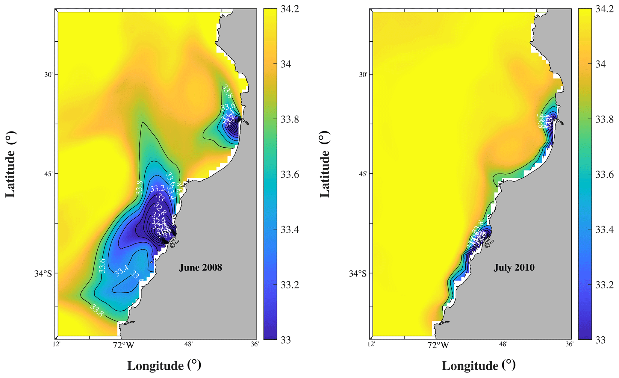
Figure 5 Salinity distribution in June 2008 and July 2010, corresponding to the changes in the wind stress direction to SSE – see Fig. 2.

The variation in the strength of the area-averaged salinity gradient (AASG) (Fig. 9) is consistent with the extension of the plumes and correlates with the total river discharges (Fig. 6), which involve stronger gradients and fronts during fall–winter.

Besides the variation in the total area, the alongshore extension was also evaluated in order to identify interannual variability in plume influence along the coast (Fig. 1). Episodes of high river discharges are normally accompanied by an extension of up to 30 km southward along the coast and coalescence of the plumes (Fig. 10), which is consistent with changes in the wind direction (Figs. 2 and 5). The years 2005, 2006 and 2008 presented a marked plume extension during austral winter, whereas the summers of the years 2005, 2007 and 2010 were characterized by a minimum or absence of the plumes along the entire coast.

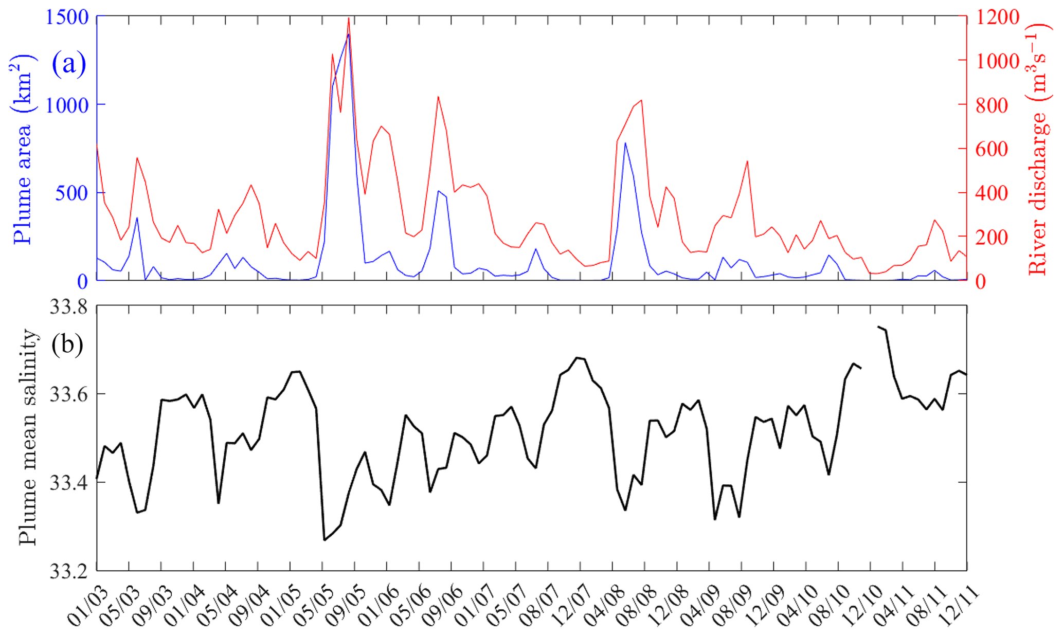
Figure 6 Variation in (a) river plume area and total river discharge and (b) mean plume salinity for the period 2003–2011. The time format is month/year.

3.2 Vertical plume pattern

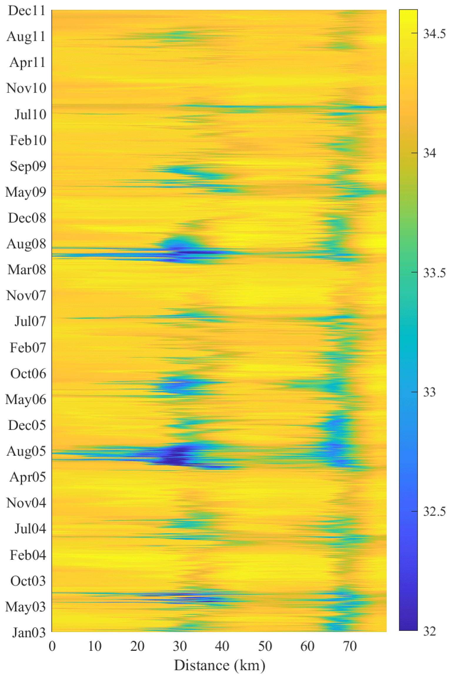
The effect of river discharges on the vertical distribution of salinity along the longitudinal transect (Fig. 1) is shown in Fig. 11. We can observe that both plumes can distribute salinity individually and there are episodes of coalescence, especially during high river discharges. Also, during some summer–fall months, the plumes are so reduced that they are not detected along this transect. If we use a salinity of 34.2 as a vertical boundary value, the plume thickness increased up to 15 m during high-river-discharge events. These events also involve a stronger stratification. The time variation along the longitudinal transect of stratification strength (Fig. 12), represented by the potential energy anomaly (PEA, J m⁻³), agrees with variations in sea surface salinity (Fig. 10) and river discharges (Fig. 6).

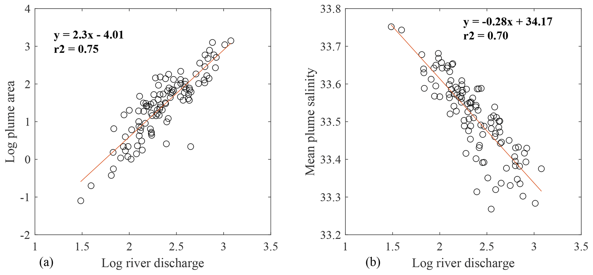
Figure 7 Scatterplot of (a) river plume area and (b) mean plume salinity as a function of total river discharge.

3.3 EOFs and wavelet

The first three modes of variability (Figs. 13 to 15) of the surface salinity are presented as follows: a map representing the EOF mode and thus, to the right, the EOF expansion coefficient (PC time series) with the related wavelet power spectrum and, further right, the cumulative wavelet spectrum. The first four modes of variability explain 66.7 %, 9.1 %, 5.5 % and 4.9 % of variability, respectively. The first mode explains the seasonal variability, as it can clearly be deduced by observing the related PC and its wavelet decomposition. The whole domain is in phase in this mode of variability; i.e., the whole system varies in the same direction (Fig. 13).

In the second mode we can observe an interesting feature, probably related to meteorological events. Here, the time series shows a high-frequency signature, with two distinct and relevant events having a period of a few months and centered in 2005 and 2010 that are probably related to particular drought events. This feature is also of interest looking at the spatial counter-phase character, as the southernmost area of the domain shows a different sign with respect to the estuaries' area. The shape of the southern plume forms a front with a southern area having a positive sign. This is linked to a low-precipitation mode that reduces the area of influence of the estuaries with their plume, with special reference to the southern one (Fig. 14). Also the direction of the plumes for this mode of variability seems to be more northward than the usual climatological NW direction, which is related to changes in the wind direction and intensity for these two particular events.

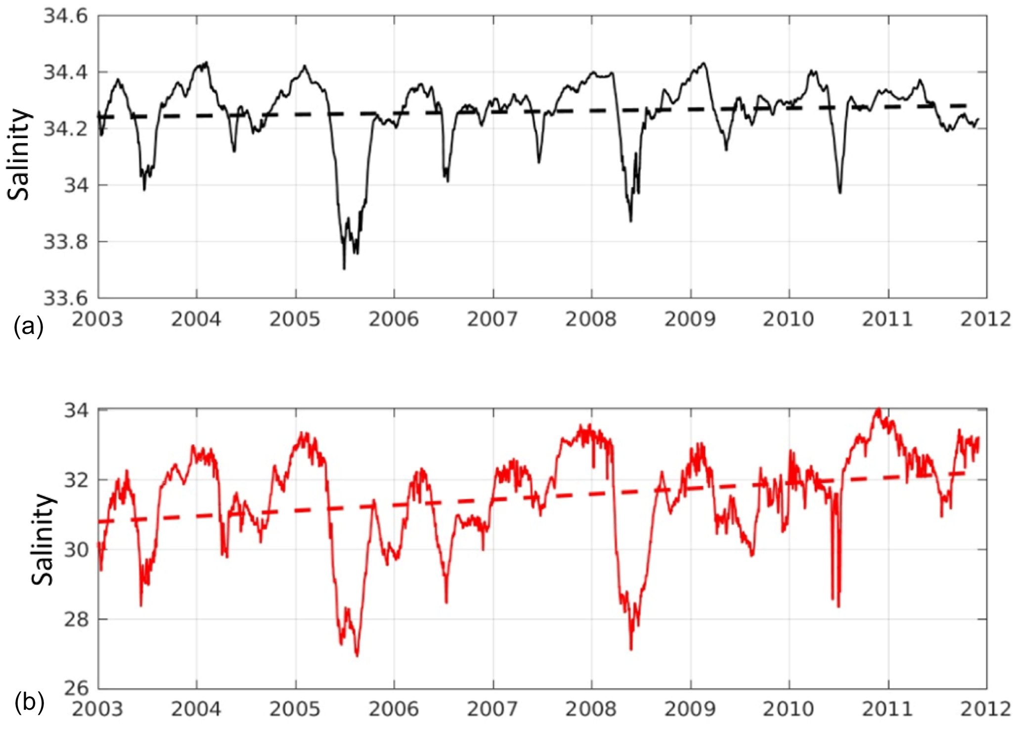
Figure 8 Time series and trends of the (a) maximum and (b) minimum surface salinity over the domain.

The third mode is related again to a high-frequency signal superimposed on a longer signal at the end of the series. This corresponds to a reduction in this signature of the plumes, where a high-frequency signature characterizes a longer-period signal most likely related to the beginning of the 2010–2015 mega-drought (Fig. 15). The most noticeable events are those shown in the second mode of variability. This feature in the spatial mode corresponds to two distinct minima of surface salinity related especially to the Rapel River plume.

For what concerns zonal and meridional velocities, we just show the first three modes of variability in the meridional component, i.e., the north–south part of the flow. The zonal component analysis does not show significant results and/or is not easy to interpret probably because the geography and morphology of the central Chile coast are dominated by the meridional component of the flow.

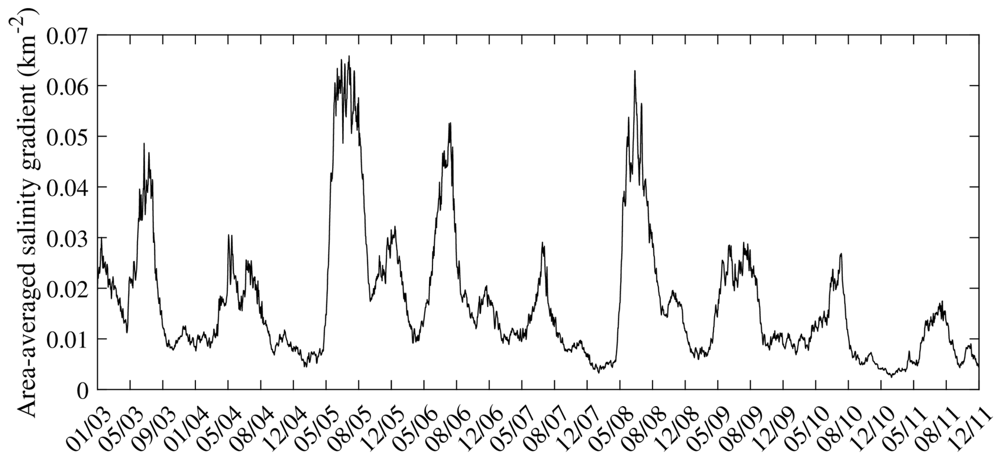
Figure 9 Variation in the area-averaged salinity gradient (AASG) in the Maipo–Rapel plume area. The time format is month/year.

The three modes, shown in Figs. 16–18, explain 42 %, 15 % and 12 % of variability, respectively, linked to the annual cycle, the semiannual cycle, and some mesoscale variability (high frequency) linked in its turn to partly semiannual and annual frequencies (i.e., the analysis put in relation to such scales that actually are interlinked by means of energy cascades). What is evident is, for all the three modes, a clear influence of the river runoff area on the spatial variability in the meridional transport.

On the other hand, at first sight, there is not a clear similarity between PCs of the salinity and the meridional-flow PCs. Considering the wavelet analysis, above all in terms of the power spectrum and cumulative spectrum, the first mode of the meridional transport (Fig. 16) shows some similarity with the spectra shown by the third EOF surface salinity variability (Fig. 15). So, a good part of the meridional transport variability, especially in the “blue” area of this first mode, could be influenced by processes linked to the third mode of the salinity, which seems related to interannual events because it is observable by frequencies of the cumulative power spectrum. It also seems that the other part of such interannual variability is also enclosed in the second mode of salinity variability, in particular for the mid-2005 event, that in salinity is evident in the second mode (Fig. 14), while in terms of meridional velocity it is separated in the third variability mode. Also in this case, the event, with a semiannual signal in terms of the cumulative spectrum, seems to have a correspondence in terms of meridional transport variations.

Figure 10 Hovmöller diagram for sea surface salinity (SSS) along a longitudinal transect (see Fig. 1) extending across the Maipo and Rapel river plumes.

4 Discussion

During the 9-year period of study, the river plumes were normally restricted to a short distance from the river mouths, where they also exhibited larger horizontal variability but a more homogeneous vertical structure close to the river mouth. In an analytical study, Hetland (2005) stated that mixing is more intense near the river mouth while wind efficiency is higher farther away, which is consistent with the plume shape and orientation in our results. Similarly, other authors have pointed out that, in the near field, the plume behaves as a buoyant jet with a stronger effect at the bottom, while in the far field, the horizontal density gradient is weaker and strongly affected by the wind and Coriolis force (Chao, 1988; Chen et al., 2009; Horner-Devine et al., 2015). In our study, we observed a strongly stratified plume even in the far field during winter months. This contrast is explained by the combination of larger river discharge and weaker wind efficiency.

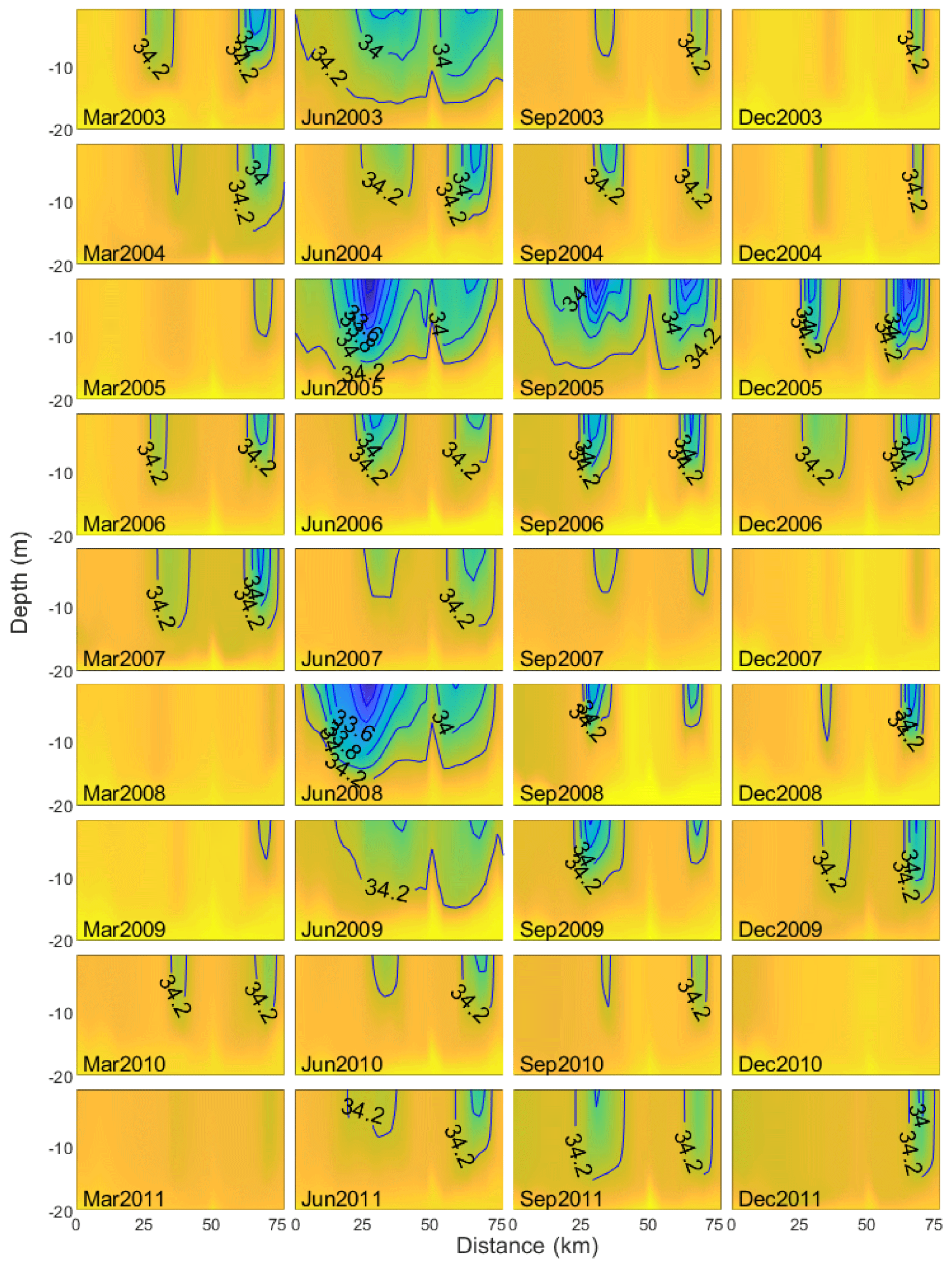
Figure 11 Vertical distribution of salinity along the longitudinal transect (Fig. 1) in the Maipo–Rapel river plume area.

Considering their relatively steep slopes and small watersheds, compared to larger rivers, the Maipo and Rapel rivers are similar to systems of small mountainous rivers that exhibit a rapid response to episodes of increase in freshwater, generating river plumes with strong stratification near the river mouth (Warrick et al., 2004). An interesting feature observed in river plumes is the occurrence of “rooted” plumes in shallow areas (Zhi et al., 2022). It is possible that this process can also occur off central Chile in winter when there is a predominance of northwesterly winds.

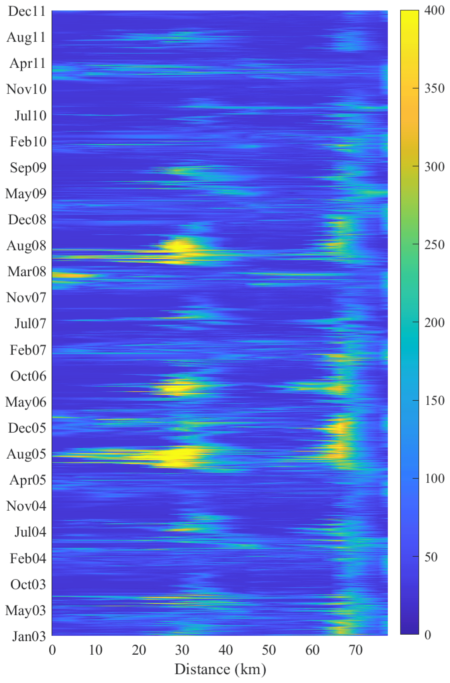
Figure 12 Hovmöller diagram for potential energy anomaly (PEA, J m⁻³) along the longitudinal transect (see Fig. 1) extending across the Maipo and Rapel river plumes.

The plume extension and mean surface salinity are strongly correlated with the river discharge, with wind playing a secondary role and mostly influencing the plume shape and orientation, as observed during two winter episodes with northwesterly winds also described elsewhere by Rojas et al. (2023). Comparing different forcing, Hickey et al. (2005) state that the extension and shape of the river plumes mostly depend on river runoff, wind and surface currents over the continental shelf, although there are other factors that influence the spread of river discharge, like tides, characteristics of the discharge, bathymetry and Coriolis acceleration (Archetti and Mancini, 2012). For instance, Chen et al. (2017a) state that, outside the micro-tidal estuary, wind is the main forcing contributing energy for mixing the Pearl River plume over the shelf. This explains the vertical pattern observed in the Maipo–Rapel river area, in agreement with Rojas et al. (2023), where the higher PEA and stratification are observed in winter, when wind is weaker and river discharge is the most important driver of the plume dynamics, except during the northwesterly wind events.

Fernández-Nóvoa et al. (2015) showed that the river discharge had a higher variability during the period of higher discharge and when landward, downwelling-favorable winds pushed the plume to the coast, making it flow along the coast. Something similar is observed during episodes of strong NNW winds off the Maipo–Rapel rivers occurring in winter. This seasonal change in the plume extension and direction has already been described by other authors (Fiedler and Laurs, 1990; García Berdeal et al., 2002).

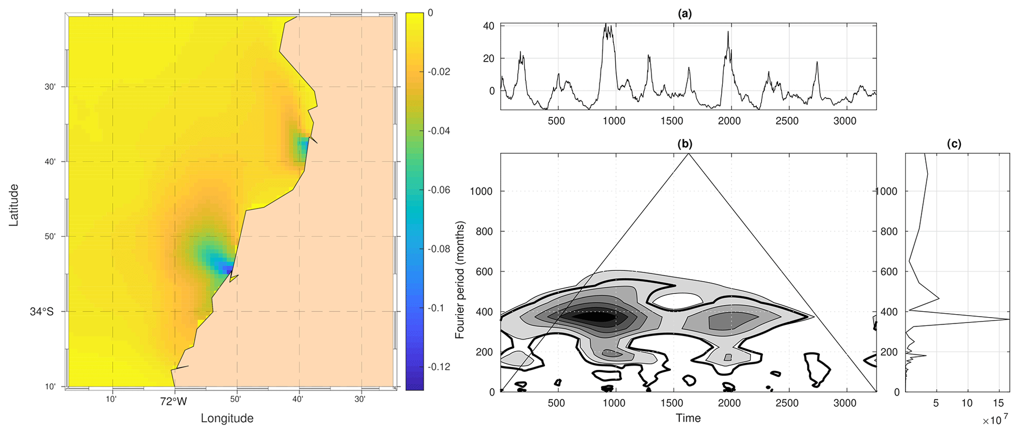
Figure 13 (Left panel) EOF Mode-1 map. (a) EOF PC-1 time series. (b) Wavelet spectrum of the PC series (time in days). (c) Cumulative global wavelet spectrum.

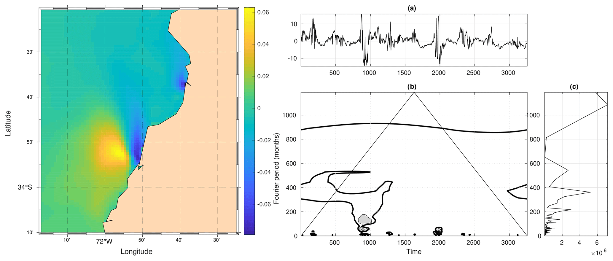
Figure 14 (Left panel) EOF Mode-2 map. (a) EOF PC-2 time series. (b) Wavelet spectrum of the PC series (time in days). (c) Cumulative global wavelet spectrum.

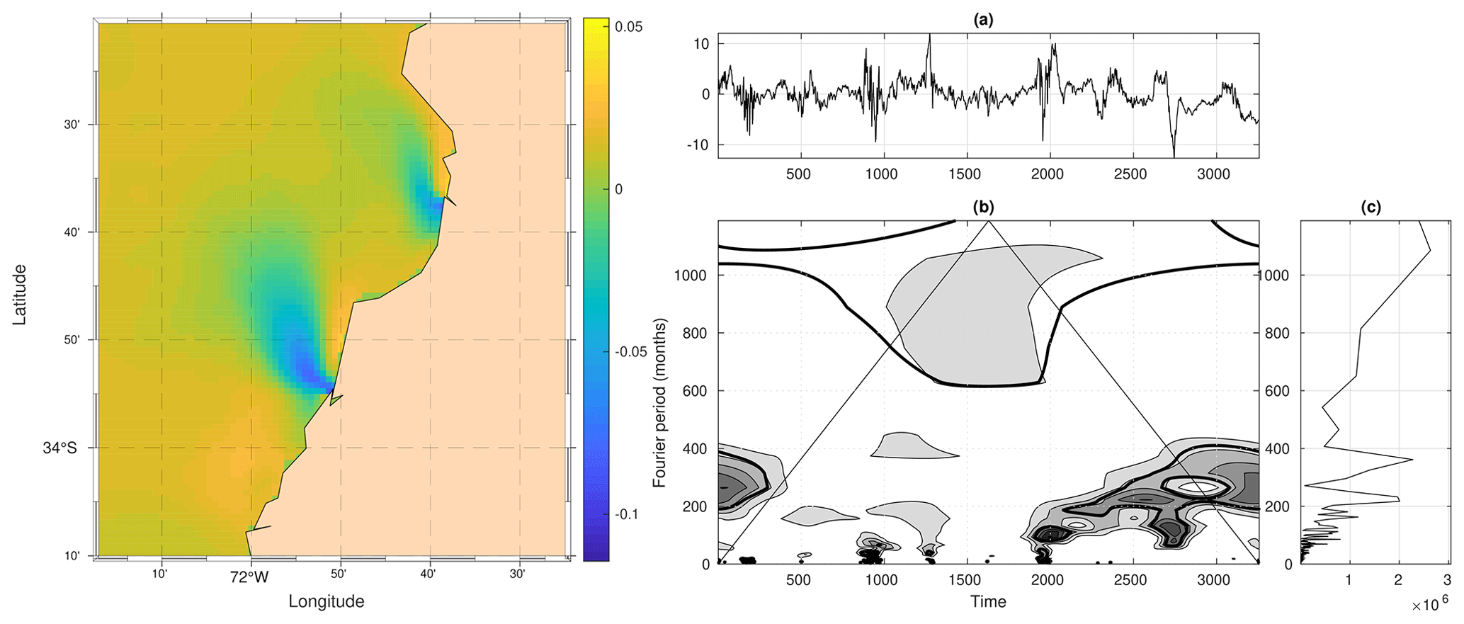
Figure 15 (Left panel) EOF Mode-3 map. (a) EOF PC-3 time series. (b) Wavelet spectrum of the PC series (time in days). (c) Cumulative global wavelet spectrum.

Subtidal currents associated with wind-influenced currents and mesoscale eddies are also an important forcing linked to the transport of river plume sediments over long distances and long timescales (Blaas et al., 2007). However, the intra-annual variability and seasonal variability remain driven by wind and river discharges, respectively, as has also been observed in other systems where river discharge controls the plume dynamics in the long term and wind is more relevant in the short term (Falcieri et al., 2014). In this sense, consistent with our results, Piñones et al. (2005) assert that the Maipo River plume is mostly driven by the river discharge in winter but the influence of wind is more important during spring–summer. Normally, the predominant wind in this region is from the southwest, decreasing its intensity in fall–winter (Strub et al., 1998) and with episodic strong storms during winter (Hernández-Miranda et al., 2003) and periods of upwelling and relaxation and intrusion of oceanic waters during summer (Letelier et al., 2009; Aguirre et al., 2012).

It is worth mentioning that 9 years is a short period to capture any significant impact by the PDO in the study area (although it shows a clear interannual variability which correlates with the El Niño–Southern Oscillation, ENSO). However, the impact of El Niño and La Niña showed marked contrasting effects on turbid river plumes off central-southern Chile during the period of study (e.g., Saldías et al., 2016). In fact, the years of 2005 and 2006 were very wet periods with anomalously high rainfall and peaks in river discharges. The river plumes were anomalously big during those years in response to the freshwater availability. In fact, these conditions promoted flooding events in central Chile. In contrast, periods such as 2007 and 2011 were characterized by anomalously low signatures of freshwater plumes from the satellite observations, which coincided with the influence of La Niña and a lack of rainfall in central-southern Chile (Saldías et al., 2016). In this sense, Hernandez et al. (2022) pointed out that, even though some catchments are strongly correlated to ENSO with related hydro-climatic anomalies, mixed regimes do not exhibit a clear connection. On the other hand, Alvarez-Garreton et al. (2021) stated that snow-dominated catchments are especially vulnerable to long-term droughts, showing the accumulated effect from previous years; this could be reflected especially in a reduction in the plumes' extension during spring–summer, as observed after 2008 (Fig. 6). This long-term drought has been described by other authors (Winckler et al., 2020) and is attributed to anthropogenic climate change, with an evident decrease in river discharges in central Chile since 2010.

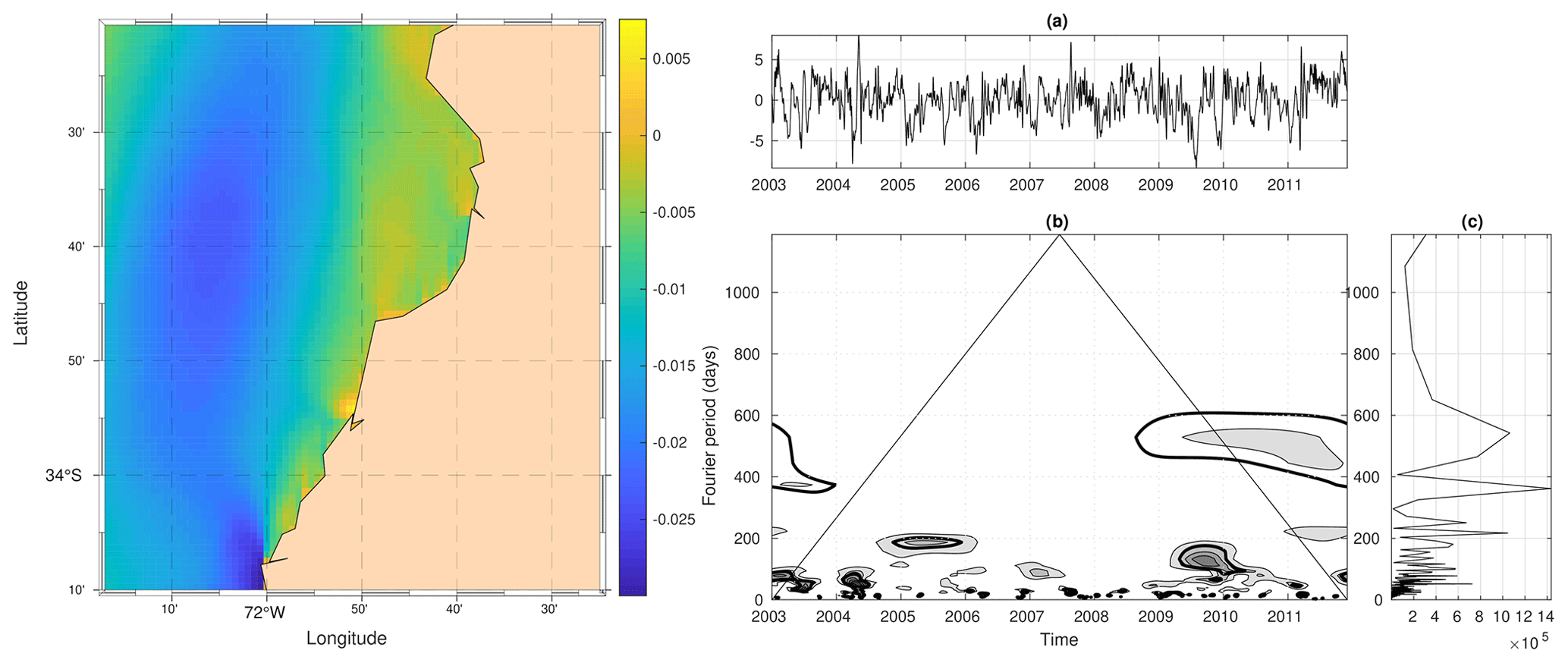
Figure 16 (Left panel) Meridional-velocity EOF Mode-1 map. (a) EOF PC-1 time series. (b) Wavelet spectrum of the PC series (time in days). (c) Cumulative global wavelet spectrum.

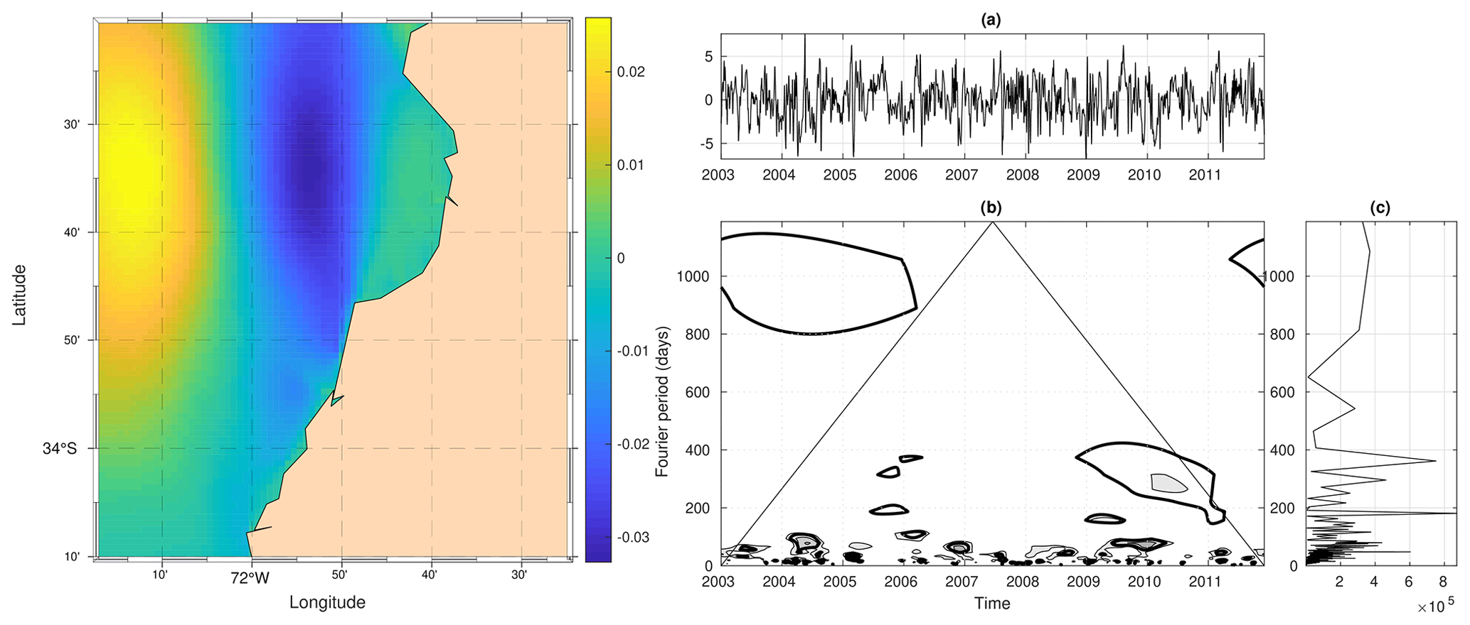
Figure 17 (Left panel) Meridional-velocity EOF Mode-2 map. (a) EOF PC-2 time series. (b) Wavelet spectrum of the PC series (time in days). (c) Cumulative global wavelet spectrum.

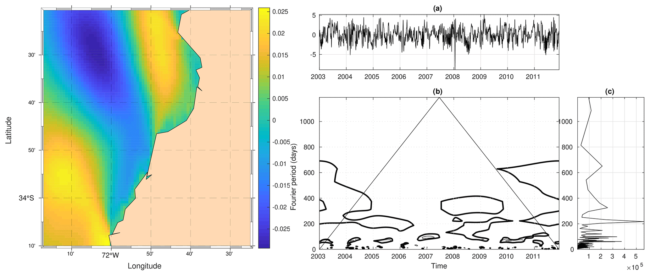
Figure 18 (Left panel) Meridional-velocity EOF Mode-3 map. (a) EOF PC-3 time series. (b) Wavelet spectrum of the PC series (time in days). (c) Cumulative global wavelet spectrum.

The pattern here described is opposite to the interannual and seasonal variability in the Columbia River. Here, Burla et al. (2010) and Chen et al. (2017a) described a northward plume attached to the coast in winter and a detached plume in summer, detaching that is normally observed during events of wind relaxation or wind reversal. Moreover, Chen et al. (2017b) asserted that upwelling jets are able to transport river plumes long distances along the coast. However, whereas the Columbia River has a snow-dominated regime where a maximum river discharge coincides with a period of intense upwelling-favorable winds, river plumes in central Chile are characterized by a phase difference between higher freshwater discharge and stronger upwelling-favorable winds. The detachment of the plumes (northwestward direction) observed during summer in this study is in agreement with Ekman theory, as described by Rojas et al. (2023) and Saldías et al. (2012), where upwelling-favorable wind forces the detachment and direction of the buoyancy-driven plume.

An interesting point to consider is the conclusion by Berghuijs et al. (2014), who stated that a shift from snow- to rain-dominated regimes in some catchments would lead to a decrease in the mean streamflow. In pluvio-nival regimes like that of the Rapel and Maipo rivers, this would mean that plumes extending over coastal areas would mostly depend on the river discharges occurring in winter. In this sense, Döll and Schmied (2012) modeled climate change projections and asserted that low flows could decrease up to 50 % and some systems could even change their regime from perennial to intermittent.

As described by Garreaud and Falvey (2009), it is expected that future conditions in this region will be characterized by stronger southerly winds, which would involve the Rapel and Maipo rivers being able to extend further north and closer to the coast. On the other hand, projections also predict a southward extension of the semi-arid climate (Winckler et al., 2020), which means that the river discharges in this region would tend to decrease over time. Thus, we expect that smaller river plumes would extend closer to the coast and probably have an impact on the distribution of benthic communities and larval stages (Grimes and Kingsford, 1996), besides a possible impact on the sand supply to beaches that strongly depend on these rivers and that already show progressive erosion and shoreline retreat (Martínez et al., 2018, 2022). Although not explored in this study, it is evident that ENSO hydro-climatic anomalies have a strong influence on the hydrological regime (Hernandez et al., 2022) and the river plume structure along the continental shelf off central-southern Chile (Saldías et al., 2016). Consequently, it is expected that changes in the pattern described here during the coming decades will be observed.

Although the model does not include the wave effect, further studies should consider this variable as most of the plume remains attached to the coasts, especially during high-energy wave events in winter. In this sense, Delpey et al. (2014) describe the strong effect that waves can have on the river plume dynamics, including alongshore currents and flushing time. A recent study on the Maipo River plume also demonstrates the strong influence that waves can have on plume dynamics in shallow areas (Flores et al., 2022).

5 Conclusions

The hydrography of the area influenced by the Maipo and Rapel river plumes was modeled for the period 2003–2011, where a strong dependence of the plumes' features on freshwater discharge and wind forcing could be evidenced. Unlike other systems like the Columbia River, a larger extent, lower mean salinity and stronger stratification are observed in wintertime, when wind is weaker and sometimes downwelling-favorable; in spring–summer, when upwelling-favorable wind is stronger, these river plumes are smaller and their stratification is weaker, which is consistent with previous studies. Strong, downwelling-favorable events are able to reverse the river plume direction and push it southward to form a narrow band attached to the coast. The EOF analysis confirmed the strong seasonality of the Maipo–Rapel river plume system. A second mode showed an intra-annual signal, likely associated with meteorological events, which also exhibited a contrasting north–south spatial sign.

An increasing trend of mean salinity was observed in the study domain, associated with a decreasing trend in river discharges. This trend corresponds to the beginning of the 2010–2015 mega-drought exhibited by this region. No correlation was found between the plumes characteristics and El Niño–Southern Oscillation (ENSO) and Pacific Decadal Oscillation (PDO) indices, which can be explained by the complexity of mixed regimes and the fact that snow-melting regimes show a lag from and cumulative response to previous years. It is possible to speculate that a shift from snow- to rain-dominated regimes, along with changes in wind and precipitation patterns, will be reflected in smaller river plumes and will be more attached to the coast, along with an increase in local mean surface salinity, which would affect planktonic and benthic communities.