Relative dispersion and kinematic properties of the coastal submesoscale circulation in the southeastern Ligurian Sea

An array of Lagrangian instruments (more than 100 drifters and a profiling float) were deployed for several days in the coastal waters of the southeastern Ligurian Sea to characterize the near-surface circulation at the submesoscale (< 10 km). The drifters were trapped in an offshore-flowing filament and a cyclonic eddy that developed at the southwestern extremity of the filament. Drifter velocities are used to estimate differential kinematic properties (DKPs) and the relative dispersion of the near-surface currents on scales as small as 100 m. The maximum drifter speed is ∼ 50 cm s⁻¹. The DKPs within the cluster exhibit considerable spatial and temporal variability, with absolute values reaching the order of magnitude of the local inertial frequency. Vorticity prevails in the core of the cyclonic eddy, while strain is dominant at the outer edge of the eddy. Significant convergence was also found in the southwestern flow of the filament. The initial relative dispersion on small scales (100–200 m) is directly related to some of the DKPs (e.g., divergence, strain and instantaneous rate of separation). The mean squared separation distance (MSSD) grows exponentially with time, and the finite-size Lyapunov exponent (FSLE) is independent of scale. After 5–10 h of drift or for initial separations greater than 500 m, the MSSD and FSLE show smaller relative dispersion that decreases slightly with scale.

1 Introduction

Coastal filaments and eddies play an important role in the transport between coastal and deep open-sea waters and are therefore critical to the local ecosystem dynamics and fisheries. They can be quite small (< 10 km, hereafter referred to as submesoscale) and evolve rapidly at daily or smaller timescales. They can be seen in satellite imagery of coastal areas, especially where rivers discharge water with different physical (e.g., temperature) or biological (e.g., chlorophyll or dissolved organic matter) properties into the sea. Examples of coastal filaments and eddies detected by satellite imagery of sea surface temperature or chlorophyll concentration and observed by in situ measurements in the oceans and semi-enclosed seas can be found in numerous publications (e.g., Flament et al., 1985; Wong et al., 1988; Zatsepin et al., 2003; Poulain et al., 2004, 2020; Schroeder et al., 2011, 2012; Schaeffer et al., 2017).

In situ observations of coastal dynamics using traditional methods based on surveys with research vessels and moored instruments are not ideal for sampling high-frequency and small-scale dynamics, especially when there are hazards or limitations due to local fisheries and other coastal maritime activities. An alternative approach is to use numerous, low-cost, freely drifting (Lagrangian) instruments deployed rapidly in a specific area and tracked over time (e.g., Mahadevan et al., 2020; D'Asaro et al., 2018). Such a sampling strategy was adopted off Livorno (Italy) in the southeastern Ligurian Sea (SLS; Fig. 1) in October 2020 to provide three-dimensional (3D) spatial characterization and rapid temporal monitoring of the coastal environment at scales as small as ∼ 100 m (Poulain, 2020).

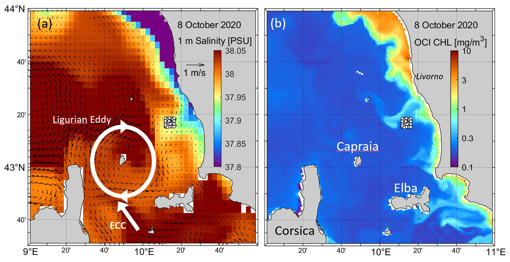
Figure 1 (a) CMEMS near-surface currents (arrows) and salinity (colors) and (b) MODIS chlorophyll concentration (OCI algorithm) on 8 October 2020 at 12:00 UTC in the SLS. The Italian mainland is to the east. The drifter deployment locations are indicated with white dots (6 × 6 km² array). The ECC and Ligurian Eddy are schematized in white.

Circulation in the SLS is dominated by the East Corsica Current (ECC), which flows northward between the islands of Corsica and Elba (Fig. 1). The ECC varies seasonally (Astraldi and Gasparini, 1992) and is also characterized by velocity fluctuations with periods of 2–15 d with intermittent reversals (Astraldi et al., 1990). The ECC generally rotates clockwise around the island of Capraia, forming an anticyclonic eddy centered on the island (Poulain et al., 2012; Ciuffardi et al., 2016; Iacono and Napolitano, 2020). This Ligurian Eddy or Capraia Eddy is dominant in summer when the ECC is weak (Iacono and Napolitano, 2020). Coastal circulation and dispersion in the SLS region have been described using ocean color satellite imagery and drifter data (Schroeder et al., 2012; Poulain et al., 2020). Coastal currents were shown to vary strongly with local winds, including intermittent complete reversals in direction. Coastal dispersion was found to be 1 order of magnitude larger than in the offshore Ligurian Sea and was significantly underestimated by numerical ocean circulation simulations (Schroeder et al., 2012).

The objective of this work is to describe the spatial structure and temporal evolution of a particular submesoscale offshore-flowing filament and a small cyclonic eddy sampled by Lagrangian drifters in the coastal SLS, focusing on the local surface dispersion and the kinematic properties of the surface currents. The circulation and dispersion measured by the drifters during a short period of 2 d are described using a mix of Lagrangian and Eulerian metrics. First, relative dispersion is evaluated by calculating the mean squared separation distance (MSSD) of drifter pairs and by estimating the scale-dependent finite-size Lyapunov exponent (FSLE). The MSSD and FSLE results are compared qualitatively with the theoretical dispersion regimes of two-dimensional geophysical turbulence. Second, Eulerian maps of surface currents are produced using an optimum interpolation technique, and differential kinematic properties (DKPs) of the flow are computed.

The experimental site was chosen to be east of the ECC and Ligurian Eddy, about 15 km from the Italian coast (Fig. 1), south of the major industrial port of Livorno and south of a floating regasification terminal. Monitoring and predicting currents and dispersion in this area are important due to the higher probability of accidental releases of pollutants in the coastal waters. A cloud-free Moderate Resolution Imaging Spectro-radiometer (MODIS) chlorophyll concentration image taken on 8 October 2020 reveals several coastal filaments and eddies transporting nutrient-rich water offshore from the Italian coast. In particular, a filament extending tens of kilometers in the southwest direction prevails near the northwestern edge of the drifter deployment array. On the same day, operational numerical simulations provided by the Copernicus Marine Environment Monitoring Service (CMEMS) show a well-defined coastal area with fresher water to the east and north of our experimental site, mainly due to the outflow of the Arno River near Livorno. CMEMS currents are rather weak (< 10 cm s⁻¹) in this coastal area. In contrast, a noteworthy meandering ECC and Ligurian Eddy dominate the near-surface circulation offshore (Fig. 1).

More than 100 drifting instruments deployed quickly in a small array on the morning of 8 October 2020 were used to study the near-surface relative dispersion and kinematic properties of an offshore-flowing filament and cyclonic eddy. Additional drifters and a float were deployed to provide ancillary data on surface waves and vertical profiles of temperature, salinity and currents. All the drifting instruments deployed during the experiment are briefly described in Sect. 2, including information on their deployments and the processing of their data. Data analysis methods are also described. Results are presented and discussed in Sect. 3, focusing on the kinematic properties of the near-surface circulation and lateral relative dispersion. The results are discussed and conclusions are drawn in Sect. 4.

2 Data and methods

2.1 Lagrangian instruments

The drifters and profiling float used in the coastal SLS are described in detail in Poulain (2020). Only a summary is provided below. Most drifters were Coastal Ocean Dynamics Experiment (CODE; Davis, 1985), Consortium for Advanced Research on Transport of Hydrocarbon in the Environment (CARTHE; Novelli et al., 2017) and Palo Alto Research Centre (PARC; Waterston et al., 2019; Cocker et al., 2022) drifters using GlobalStar or Iridium satellite telemetry systems. Global Positioning System (GPS) positions were measured every 5 to 20 min. They measured surface currents within 1 m of the sea surface. The effects of wind and waves on the motion of CODE and CARTHE drifters are comparable (Poulain et al., 2022). The main error is a wind-induced slip of about 0.1 % of the wind speed (Poulain and Gerin, 2019). The wind- and wave-induced slip of the PARC drifters has not yet been studied. A total of 50 CODE, 20 CARTHE (Berta et al., 2021) and 30 PARC drifters were deployed.

Additional Lagrangian instruments included (1) the RIVER drifter, a CODE-like drifter equipped with a down-looking acoustic Doppler current profiler (ADCP) to measure relative current profiles between 2 and 20 m depth with a vertical resolution of 1 m; (2) the Surface Velocity Program (SVP) drifter (Niiler, 2001) with a drogue centered at 15 m nominal depth; (3) the directional wave spectra (DWS) drifter (Centurioni et al., 2017) to measure the directional statistical properties of the surface wave; and (4) the Arvor-C float (André et al., 2010) to measure temperature and salinity profiles with a pumped conductivity, temperature and depth (CTD) sensor between the surface and ∼ 120 m depth with 1 m vertical resolution. Five SVP, two RIVER and three DWS drifters were operated.

The GPS position data of the drifters were quality controlled and interpolated at 0.5 h intervals using a kriging technique (Menna et al., 2017, and references therein). Velocities were calculated by finite differencing the interpolated positions (central difference with hourly interval).

2.2 Remotely sensed data and operational products

MODIS satellite images of the chlorophyll concentration of the study area were used to describe the spatial structure and temporal evolution of the surface circulation assuming that chlorophyll is a passive tracer advected by the surface horizontal currents. As previously shown in Poulain et al. (2020), chlorophyll concentration images were preferred over sea surface temperature images as they better represent circulation features. Since we are in a coastal area where a river drains nutrient-rich water, there is a sharp contrast between coastal and offshore water, with the former being richer (higher chlorophyll) and more turbid. Daily images have a horizontal resolution of 1 km.

Atmospheric data (wind speed and direction 10 m a.s.l.) and surface wave data (significant wave height, main wave period and direction, Stokes drift) of the fifth-generation European Centre for Medium-Range Weather Forecasts (ECMWF) reanalysis (ERA5) for the global climate and weather were downloaded from the Copernicus Climate Data Store for October 2020 in the SLS. They are provided with a horizontal resolution of 0.25^∘ (wind) and 0.5^∘ (waves). CMEMS reanalysis products at $\mathrm{1}/\mathrm{24}$th degree (∼ 4 km) horizontal resolution were also downloaded. Simulated hourly mean currents at the sea surface were used.

2.3 Deployment strategy

In situ data were collected as part of the Drifter Demonstration and Research 2020 (DDR20) experiment (Poulain, 2020), which took place off the coast of Italy on 8–10 October 2020. DDR20 was a rapid environment assessment (REA) exercise whose general objective was the 3D characterization of the oceanographic and acoustic environment using a network of compact and low-cost, freely drifting instruments over a few days. A total of 110 drifters and 1 float were quickly deployed in a 6 × 6 km² array in the coastal LSL (Fig. 1) using two ships between 08:09 and 12:28 UTC on 8 October 2020. The minimum distance between drifters at release was 0.5 km if drifters deployed at the same time and position are not considered (Poulain, 2020). One-third of these drifters and the float were successfully recovered after about 2 d, starting at 09:22 UTC on 10 October 2020.

The experiment took place after a storm with westerly winds and waves up to 15 m s⁻¹ and 2.5 m, respectively, on 7 October (Fig. 2). During the 2 d of drifter operations mentioned above, calm meteorological conditions prevailed with winds less than 5 m s⁻¹ and waves less than 0.5 m significant wave height. The surface Stokes drift estimated by ERA5 was as large as 20 cm s⁻¹ on 7 October but decreased (to a few cm s⁻¹) on subsequent days. Note that ERA5 underestimates the significant wave height by up to 0.5 m compared to the DWS drifter measurements (Fig. 2).

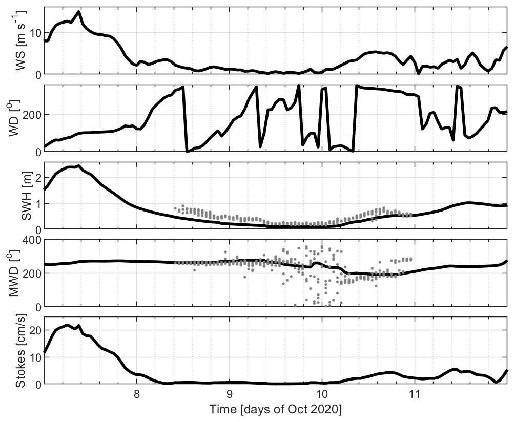
Figure 2 ECMWF ERA5 atmospheric and surface wave products at 43^∘ N, 10^∘ E (black curves): 10 m wind speed (WS) and direction (WD), significant wave height (SWH), mean wave direction (MWD), and surface Stokes drift. The surface properties measured by the DWS drifters are superimposed with gray dots. Wind and wave direction are clockwise from true north (from).

Unfortunately, 28 CODE drifters experienced transmission problems and did not transmit on 8 October between 14:00 and 22:00 UTC (∼ 8 h data gap) and between 9 October 10:00 UTC and 10 October 03:00 UTC (∼ 17 h data gap). Since the winds, waves and Stokes drift were relatively weak during the experiment, all CODE, CARTHE and PARC drifters were merged to investigate the kinematics and dispersion of the near-surface currents.

2.4 Analysis methods

The relative dispersion of a drifter cluster can be quantified using both the MSSD as a function of time after deployment, D²(t), and the FSLE versus scale (Lacorata et al., 2001; Schroeder et al., 2011, 2012; Corrado et al., 2017; Boffetta et al., 2020). Unlike the MSSD, for which pair separation is averaged at a given time, the FSLE computes the averages of separation times at a given separation distance. Thus, it has the advantage of isolating different rates of dispersion due to velocity fluctuations at a given scale. The MSSD of drifter pairs is defined as

$$\begin{array}{}\text{(1)}& D^{\mathrm{2}}\left(t\right)=<\left|{\mathit{x}}^{\left(\mathrm{1}\right)}\right(t)-{\mathit{x}}^{\left(\mathrm{2}\right)}(t){|}^{\mathrm{2}}>,\end{array}$$

where the superscripts denote the two drifters of the pair that are located at vector position x(t) at time t, and the brackets denote the average over all pairs with the same initial spacing. The time derivative of the MSSD is referred to as the relative diffusivity. The FSLE, λ, is inversely proportional to the average time, < τ >, for two drifters initially separated by δ_o to reach a prescribed separation, δ_f :

$$\begin{array}{}\text{(2)}& \mathit{\lambda }\left(\mathit{\delta }o,\mathit{\delta }f\right)={\displaystyle \frac{\mathrm{1}}{〈\mathit{\tau }〉}}\ln (\mathit{\delta }f/\mathit{\delta }o).\end{array}$$

Following Schroeder et al. (2011), we chose an amplification factor δ_f/δ_o= 1.2. The average time < τ > is often called the doubling time even though the amplification factor is not necessarily equal to 2.

The FSLE can be sensitive to the temporal resolution of the drifter positions, especially at a small separation distance for which the doubling time approaches the sampling time interval. Several methods have been proposed to reduce this problem (Boffetta et al., 2000; Lumpkin and Elipot, 2010; Haza et al., 2014). In this study, we have adopted two methods. For the first one, the drifter data were linearly interpolated using small time steps of 0.01 h before estimating the doubling times and averaging them. The second one was proposed by Boffetta et al. (2000). The following equation (see Eq. A4 in the Appendix of their paper) was used with the original drifter positions sampled at 0.5 h intervals:

$$\begin{array}{}\text{(3)}& \mathit{\lambda }\left(\mathit{\delta }o,\mathit{\delta }f\right)={\displaystyle \frac{\mathrm{1}}{〈\mathit{\tau }〉}}<\ln \left(\mathit{\delta }f\right(\mathit{\tau })/\mathit{\delta }o)>.\end{array}$$

Relative dispersion by two-dimensional geophysical turbulence has the following dispersion regimes: exponential (D² ∼ e^αt, λ= constant), Richardson (D² ∼ t³, λ ∼ ${\mathit{\delta }}^{-\mathrm{2}/\mathrm{3}}$), ballistic (D² ∼ t², λ ∼ δ⁻¹) and diffusive (D² ∼ t, λ ∼ δ⁻²) (Schroeder et al., 2012; Corrado et al., 2017).

To describe the small-scale surface circulation following the cluster of drifters, their motions with respect to the center of mass of the cluster were considered, and the DKPs of the surface currents were calculated. The DKPs of a flow describe how the surface water can decrease or increase in area, how it can rotate, and how it can be stretched or sheared (Okubo, 1970; Okubo and Ebbesmeyer, 1976; Molinari and Kirwan, 1975). They are defined by a first-order Taylor expansion of the velocity field:

$$\begin{array}{}\text{(4)}& {\displaystyle }u=(\mathit{\delta }+{\mathit{\sigma }}_n)/\mathrm{2}x+({\mathit{\sigma }}_{\mathrm{s}}-\mathit{\zeta })/\mathrm{2}y,\text{(5)}& {\displaystyle }v=({\mathit{\sigma }}_{\mathrm{s}}+\mathit{\zeta })/\mathrm{2}x+(\mathit{\delta }-{\mathit{\sigma }}_n)/\mathrm{2}y,\end{array}$$

with the following DKPs: divergence ($\mathit{\delta }=\partial u/\partial x+\partial v/\partial y$), vorticity ($\mathit{\zeta }=\partial v/\partial x-\partial u/\partial y$), shearing deformation rate (${\mathit{\sigma }}_{\mathrm{s}}=\partial v/\partial x+\partial u/\partial y$) and stretching deformation rate (${\mathit{\sigma }}_n=\partial u/\partial x-\partial v/\partial y$), where u and v are the zonal and meridional velocity components; x and y are the zonal and meridional coordinates, respectively, in the system of reference moving with the center of mass of the cluster.

Other metrics like the strain (ρ= [${\mathit{\sigma }}_{\mathrm{s}}^{\mathrm{2}}+{\mathit{\sigma }}_n^{\mathrm{2}}$]${}^{\mathrm{1}/\mathrm{2}}$), Okubo–Weiss parameter (OW $={\mathit{\rho }}^{\mathrm{2}}-{\mathit{\zeta }}^{\mathrm{2}}$) and instantaneous rate of separation (IROS $=\mathit{\delta }+\mathit{\rho }$) were also estimated. The OW measures the relative importance of strain and vorticity: elliptic regions (OW < 0) are dominated by rotation, whereas hyperbolic regions (OW > 0) are dominated by strain and deformation (Provenzale, 1999; D'Ovidio et al., 2009). The IROS is the zero-order Lagrangian rate of separation at the initial time (Schaeffer et al., 2017; Lorente et al., 2021) and is therefore related to the dispersion statistics defined above, particularly the initial exponential spreading.

There are two approaches to estimating the DKPs of horizontal currents. In the first method, small clusters of n drifters (with n > = 3) are used to solve Eqs. (4) and (5) using least squares (Molinari and Kirwan, 1975; Essink et al., 2019; Tarry et al., 2021). In the second method, the drifter velocities are interpolated on a uniform regular grid to directly calculate the horizontal derivatives of velocities and the DKPs (Lodise et al., 2020). In this work, we chose the second method and used the Data Interpolating Variational Analysis (DIVA, Troupin et al., 2012) to interpolate drifter velocities on a regular horizontal grid with a cell size of 0.1 km and zonal and meridional correlation scales of 1 km. This particular interpolation method was preferred because it provides a better estimate of the error field. In practice, interpolated values were not considered if the relative error exceeded 50 %. Gradients were estimated by central finite differences of the interpolated velocity field.

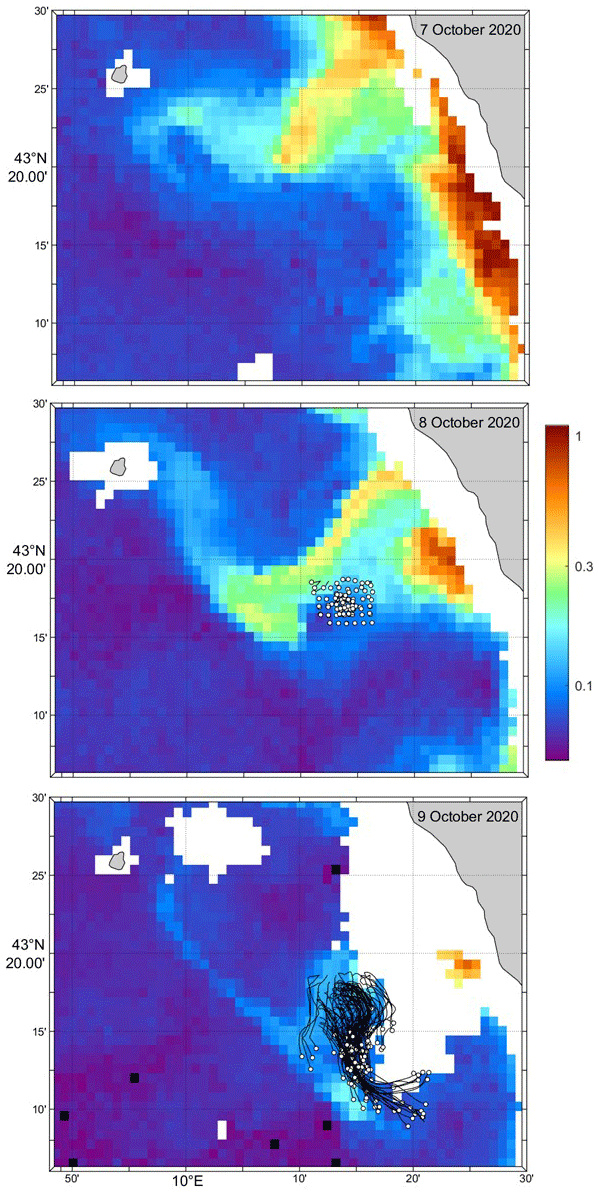
Figure 3 MODIS chlorophyll images on 7, 8 and 9 October 2020 and tracks of the drifters from deployment until 12:00 UTC on the respective days (white circles). Chlorophyll concentration is in milligrams per cubic meter (mg m⁻³).

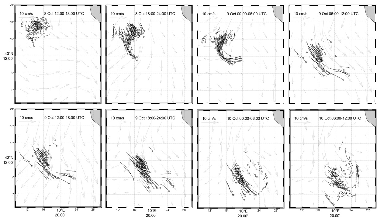
Figure 4 Track segments of all the drifters. Segments are 6 h long and end with an open circle for each drifter on the date and time posted in the panels. CMEMS surface currents are overlaid in gray for the central hour.

Uncertainties in the abovementioned statistics are due to the drifter position error, the drifter slippage and the finite number of samples. The drifter GPS positioning error can be approximated as white-noise variability with an isotropic standard deviation σ_x=σ_y ∼ 5 m (Rypina et al., 2021), uncorrelated from one drifter to another. Using a simple back-of-the-envelope calculation, the corresponding standard deviation of the squared separation distance is equal to 4${\mathit{\sigma }}_x^{\mathrm{2}}$ ∼ 100 m²= 10⁻⁴ km². Velocities estimated by finite central differencing the GPS positions interpolated or measured at dt= 0.5 h intervals have an error of σ_u= σ_v= 2${}^{\mathrm{1}/\mathrm{2}}{\mathit{\sigma }}_x/\mathrm{2}\mathrm{d}t$ ∼ 0.2 cm s⁻¹. As mentioned above, under low-wind conditions (wind speed less than 5 m s⁻¹), the drifter velocity error due to wind and waves is less than 0.5 cm s⁻¹. Hence the instrumental error of the drifter velocity is roughly 1 cm s⁻¹. The standard error of the statistics due to the finite numbers of observations can be estimated by the bootstrapping method. The 95 % confidence intervals of the MSSD and FSLE were estimated using the bootstrapping estimates of the means included in their definition (squared brackets in Eqs. 1 and 2).

Since the order of magnitude of the drifter velocities is 10 cm s⁻¹ with an error of ∼ 1 cm s⁻¹, we used a signal-to-noise ratio of 10 in the DIVA spatial interpolation. The estimation of the DKP errors estimated from the DIVA-interpolated maps is beyond the scope of this study.

3 Results

3.1 Drifter trajectories and qualitative description of the circulation

The surface drifters were released near the southern edge of a filament of coastal water extending tens of kilometers offshore. Satellite imagery (Fig. 3) shows the development and morphology of the filament whose extremities form a mushroom-like feature with anticyclonic and cyclonic eddies expanding to the north and south, respectively. The bulk of the drifters ended up in the southern cyclonic eddy. After an initial mean southward-converging drift until 9 October 00:00 UTC, they turned eastward and then northward as they diverged (Fig. 4). There is only a very qualitative agreement between the drifter velocities and the surface currents simulated by CMEMS (Fig. 4). The modeled coastal currents are essentially southeastward. At the drifter locations, they can turn toward the southwest and west, with significant differences with respect to the drifter motion. Hence, the southeast motion of the drifter cluster is more or less simulated well, but there is no signature of a cyclonic circulation in the model. In particular, on 10 October at 12:00 UTC, several drifters moved to the north, on the eastern edge of the eddy, while collocated CMEMS currents remained southeastward.

If we focus on the initial motion of the drifters, numerous surface instruments (i.e., the CODE, CARTHE and PARC drifters deployed in the central and northeastern portions of the array) moved anticyclonically with the inertial (17.55 h) or diurnal (24 h) period (Fig. 5). In contrast, SVP drifters deployed at the same locations moved directly southward, with no anticyclonic rotation. Considering the short record duration, it is not easy to separate inertial and diurnal currents. It is doubted that diurnal tidal currents are dominant in the SLS (Poulain et al., 2018). Therefore, we can speculate that the anticyclonic rotation in the tracks is the remnant of near-inertial surface currents, which were likely generated by the storm a day earlier.

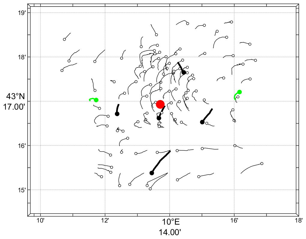
Figure 5 Tracks between 12:00 and 15:00 UTC on 8 October for all CODE, CARTHE and PARC drifters (thin curves and open circles), for the five SVP drifters (thick curves and black dots), and for the two RIVER drifters (green). Symbols are at the end of the trajectory segments. The position of the Arvor-C float during the same period is shown with a red dot. Coherent anticyclonic motions of the surface drifters contrast with the mean southward motion of the SVP drifters.

The vertical structure of thermohaline properties and currents in the area sampled by the drifters was measured by an Arvor-C profiling float and two RIVER drifters (see their initial tracks in Fig. 5). Significant shear of horizontal currents between the surface and 20 m depth was measured by the ADCP on the two RIVER drifters. The difference between the speeds at the surface and at 15 m can be up to 10 cm s⁻¹ (Poulain, 2020) and is compatible with the different motions of the CODE and SVP drifters discussed above. Temperature and salinity values measured by the Arvor-C float near the drifters (not shown) indicate a well-mixed surface layer with a temperature of about 21 ^∘C and a salinity between 37.94 and 38.00 PSU, extending down to a depth of about 40 m. At this depth, there is a sharp thermocline and a minimum salinity (Poulain, 2020). Large vertical and temporal variations of salinity associated with the offshore-flowing filament were not observed, probably because the float deployed in the center of the drifter array (Fig. 5) remained outside of the filament (see satellite image in Fig. 3).

A quick look at a velocity scatter diagram (not shown) reveals that individual drifter speeds vary in the range of 0–50 cm s⁻¹. The center of mass of the drifter cluster moved southeastward, with speeds in the range of 10–20 cm s⁻¹, and relative drifter speeds with respect to this motion had a standard deviation between 3 and 8 cm s⁻¹.

3.2 Relative surface dispersion

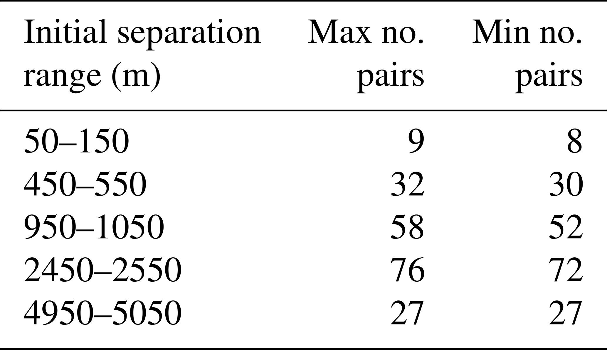
All CODE, CARTHE and PARC drifters were considered together to search for pairs near the time of deployment (8 October, 12:00 UTC) with selected separation distances of 100, 500, 1000, 2500 and 5000 m. Since the data set is limited to 10 October at 07:00 UTC and since some drifters stopped transmitting before that time, the number of pairs may decrease with time. The initial (maximum) number of pairs and the minimum number of pairs (at 07:00 UTC on 10 October) are listed in Table 1. They vary between 8 and 76.

Table 1 Maximum and minimum number of drifter pairs used to compute the relative dispersion statistics between 8 October 2020 at 12:00 UTC and 10 October 2020 at 07:00 UTC for selected separation ranges.

The surface MSSD versus time, starting at 12:00 UTC on 8 October, is shown in a log–log diagram in Fig. 6. Despite the relatively small number of pairs, the rate of change of the MSSD with time (also called relative diffusivity) during the first 10 h of drift appears to be significantly larger with the short initial spacing of 100 m than with the other larger initial distances. It can possibly be approximated by exponential growth. For longer times, the MSSD can be approximated by a power law, with the slope decreasing with increasing initial distance. However, comparison with theoretical dispersion regimes of geophysical turbulence is not straightforward. After ∼ 10 h, the MSSD values starting with separations of 100 and 500 m reach similar values near 0.8 km². Between 10 and 20 h of drift, there is a local minimum in MSSD. This decrease in relative dispersion is related to the convergence of many drifters into the small cyclonic eddy (see top panels of Fig. 4). After about a day, the MSSDs with initial separations of 100, 500 and 1000 m are all near 4 km².

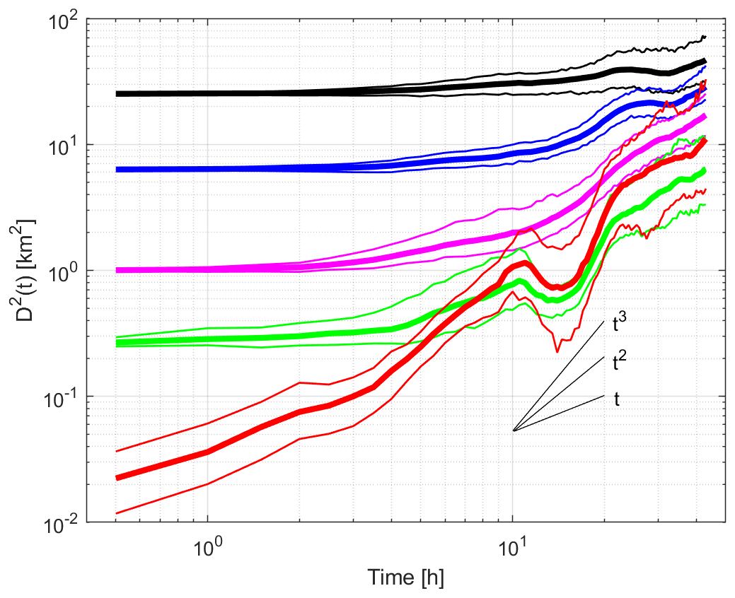
Figure 6 MSSD versus time for selected initial distances of 100, 500, 1000, 2500 and 5000 m in a log–log plot. Initial time is 8 October at 12:00 UTC. Thin curves are the bootstrapped 95 % confidence intervals. Slopes corresponding to theoretical dispersion regimes are also shown.

The FSLE for initial pair spacing between 100 m and 7 km was estimated in a similar manner, i.e., for pairs starting on 8 October at 12:00 UTC and tracked until 10 October at 07:00 UTC. The FSLE was calculated for scales divided into non-overlapping 100 m intervals using Eq. (2). The results are shown in Fig. 7 in a log–log plot, along with the number of pairs in the scale intervals. Because pairs are tracked over a limited period of 43 h, some of them do not have time to separate by the prescribed amplification factor (1.2) and do not contribute to the estimate of the average separation time, < τ >, of Eq. (1). The number of pairs whose separation increases by 120 % in less than 43 h is also shown in Fig. 7. It is generally smaller than the initial number of pairs considered, especially for large scales. The doubling time increases if the separation distance varies from 0.7 h (for small scales) to 27 h (for large scales). In general, the FSLE decreases with scale. At small scales (100–200 m), it is large (∼ 6 d⁻¹) and fairly constant. As scales increase (200–400 m), there is a strong negative slope. At larger separation distances (1–6 km), the FSLE decreases weakly with scale, with values near 0.3–0.5 d⁻¹. Again, comparison with theoretical relative dispersion slopes is not obvious. Note that the FSLE estimated using Eq. (3) (Boffetta et al. (2000) method, red curve in Fig. 7) does not differ significantly from that obtained with Eq. (2).

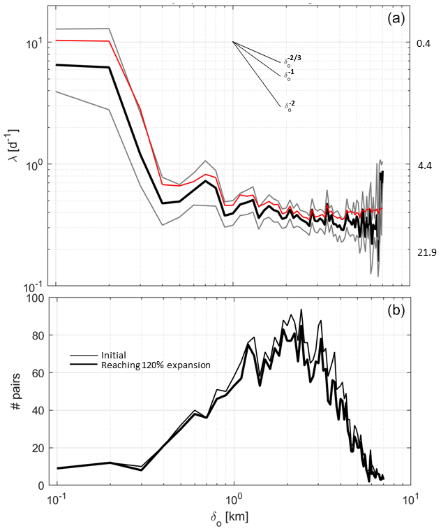
Figure 7 (a) Scale-dependent FSLE λ(δ_o) as a function of scale δ_o in a log–log plot using pairs tracked from 8 October at 12:00 UTC. The diffusive (${\mathit{\delta }}_o^{-\mathrm{2}}$), ballistic (${\mathit{\delta }}_o^{-\mathrm{1}}$) and Richardson (${\mathit{\delta }}_o^{-\mathrm{2}/\mathrm{3}}$) regimes are indicated by straight lines. Thin gray curves indicate the bootstrapped 95 % confidence intervals. Estimate using Boffetta et al. (2000)'s method (red curve). Doubling times are posted to the right in hours. (b) Number of initial pairs considered in 100 m scale bins versus the scale (thin) and the number of pairs whose separation distance was amplified by 120 % or more during the 43 h drift period (thick).

For several reasons, the confidence intervals for MSSD and FSLE displayed in Figs. 6 and 9 can be quite large. First, the number of pairs is small for small separation. Second, the distributions of squared separation distances and separation times are generally not Gaussian, and their mean values may be meaningless. Third, the drift period of 43 h is short, and the FSLE may be overestimated because a substantial fraction of pairs does not reach the 120 % amplification factor during the limited tracking period (see bottom panel of Fig. 7), and long doubling times are not considered. Nonetheless, our relative dispersion results provide some useful information, as discussed later.

3.3 Surface DKPs

We now examine the DKP maps at selected times to characterize the flow within the cluster and to monitor the shape (extent and deformation) of the area covered by the drifters. Figures 8 to 15 show the interpolated currents and the DKPs at 6 h intervals between 12:00 UTC on 8 October and 06:00 UTC on 10 October, excluding the values with more than 50 % relative error. The order of magnitude of the DKPs is equal to the local inertial frequency.

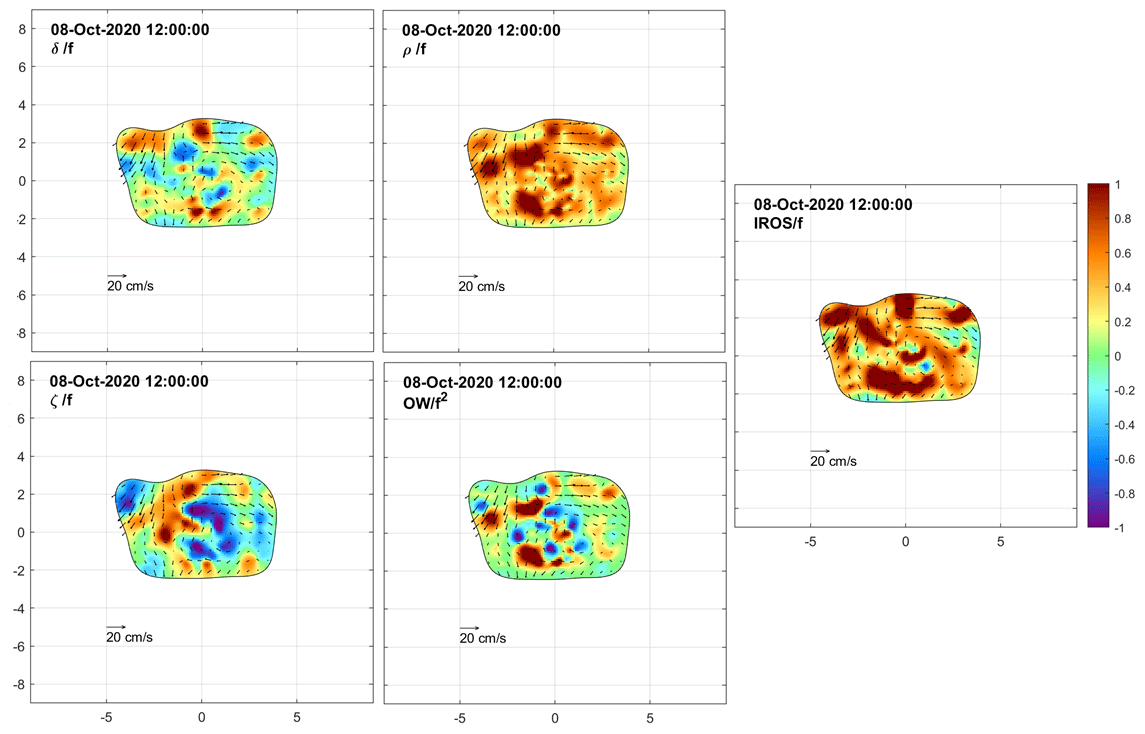
Figure 8 Maps of relative interpolated currents superimposed with color-coded DKPs on 8 October 2020 at 12:00 UTC. See text for DKP definitions. DKPs are scaled by the local inertial frequency, f. Abscissa and ordinate are in kilometers. Results with relative errors larger than 50 % are excluded.

On 8 October at 12:00 UTC, almost all the drifters were deployed, but the planned square geometry of the deployment was already modified due to the prevailing southward motion of the drifters released earlier and more to the north. As a result, the initial cluster (Fig. 8) became quasi-rectangular with sides of ∼ 6 and ∼ 8 km. Inside the sampled area, the DKPs were rather patchy. Approximately 6 h after the last deployments (at 18:00 UTC, Fig. 9), the cluster had mainly expanded in the meridional direction, mainly due to the drifters near the southern edge moving rapidly southward and showing significant convergence and strain. The size of the cluster reached 10 km, in both zonal and meridional directions.

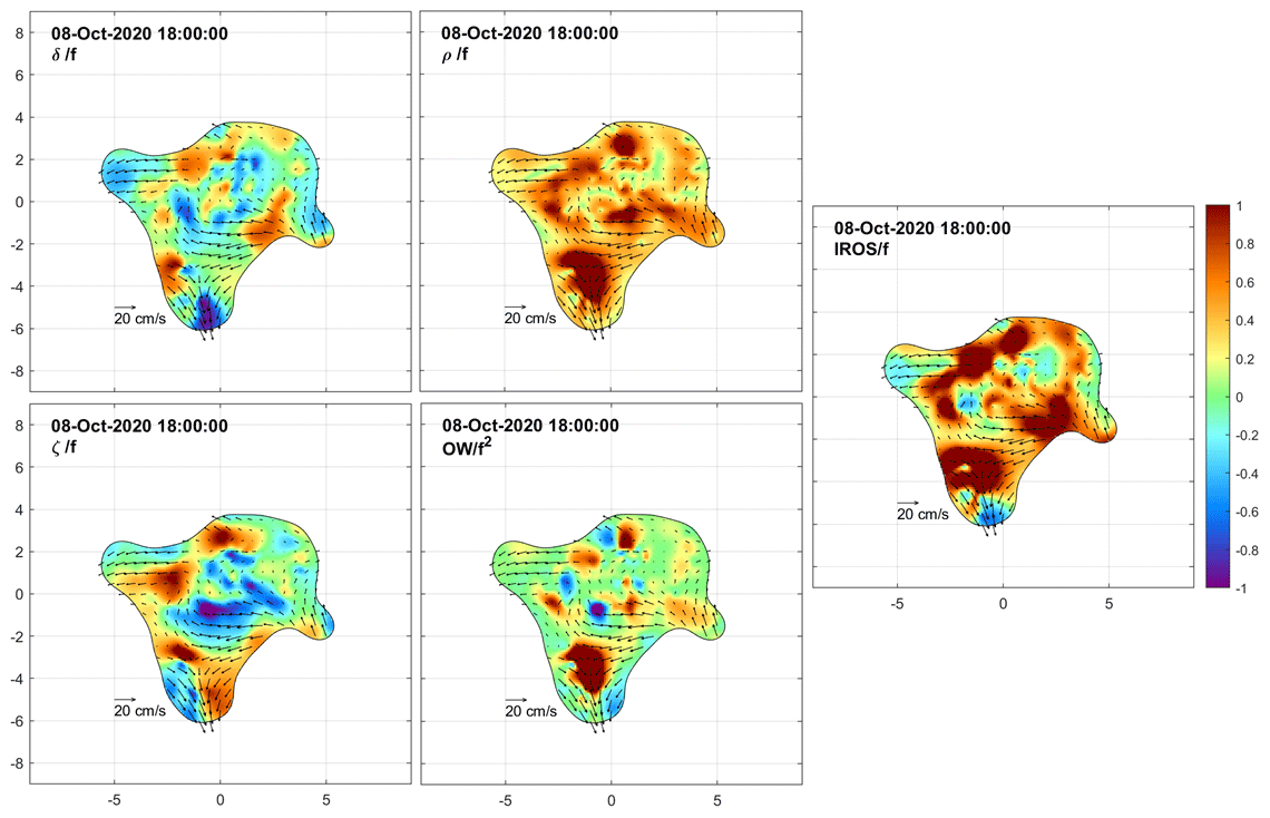
Figure 9 Same as Fig. 8 but for 8 October 2020 at 18:00 UTC.

After 6 h (Fig. 10), the northern portion of the cluster had further extended zonally, and its southern edge formed a thin branch extending southward and turning cyclonically. The divergence was generally weak. Positive vorticity prevailed east of the southward-flowing limb, while strain dominated on the opposite west side. The size of the cluster increased to ∼ 12 km in the meridional direction.

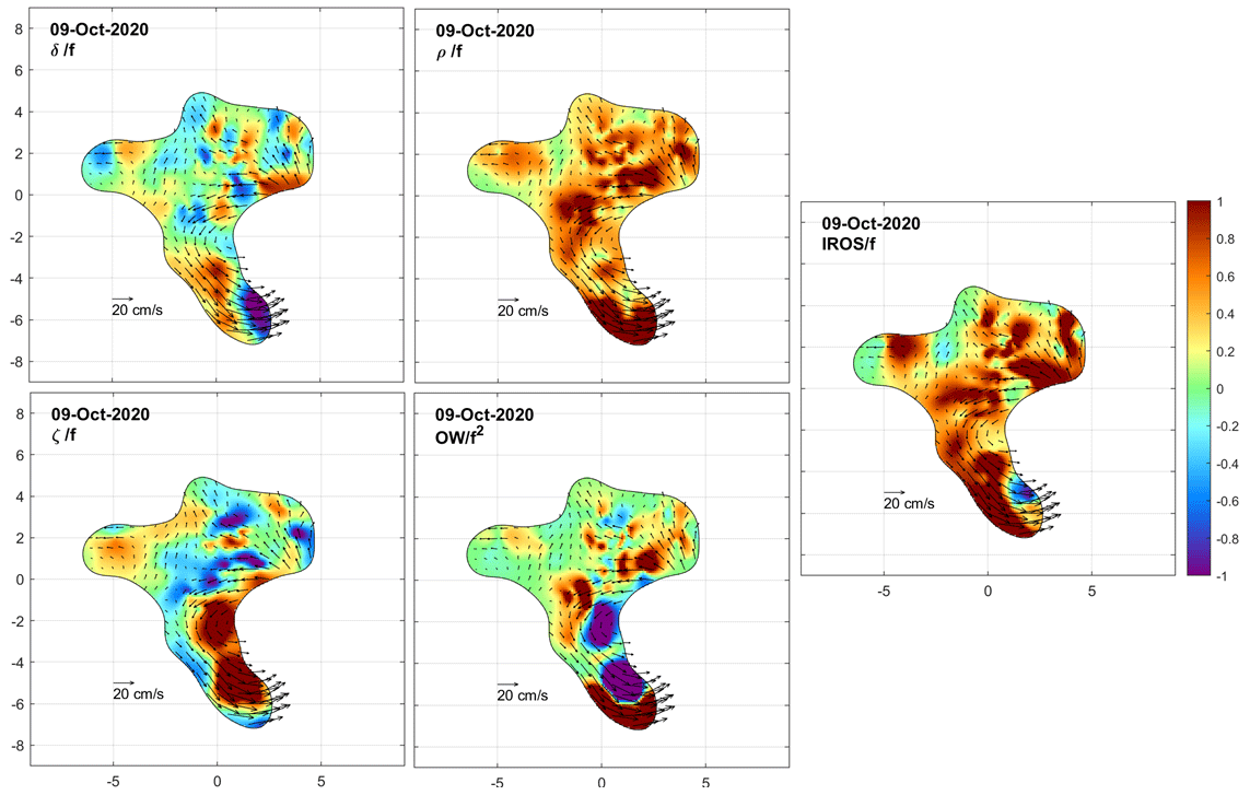
Figure 10 Same as Fig. 8 but for 9 October 2020 at 00:00 UTC.

By the morning of the next day (9 October at 06:00 UTC; Fig. 11), the southern limb had extended further in a cyclonic eddy. The divergence was patchy. A large positive vorticity exceeding f occurred in the inner part of the eddy. Outside the eddy, a hint of negative vorticity was evident. Strain was significant, especially just outside the eddy. The cluster had reached a typical size of 15 km.

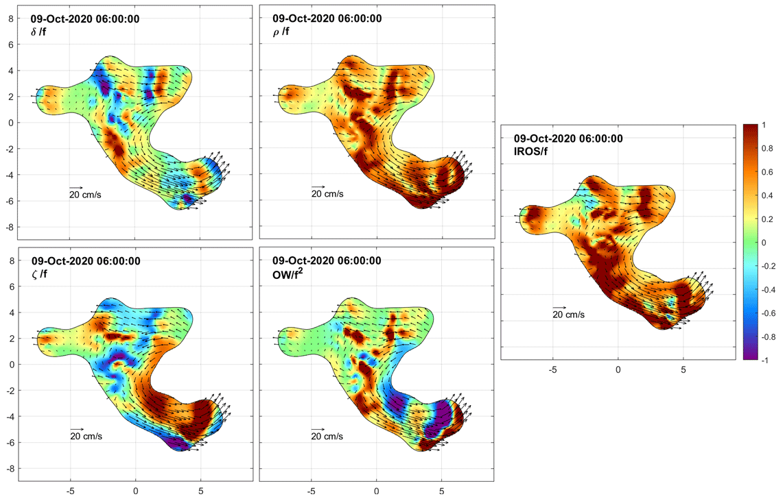
Figure 11 Same as Fig. 8 but for 9 October 2020 at 06:00 UTC.

On 9 October at 12:00 and 18:00 UTC (Figs. 12 and 13) and on 10 October at 00:00 UTC (Fig. 14), the cluster size reached a saturation value near 17 km. Some drifters moved northward and nearly closed the loop of the cyclonic eddy in its northern sector. There was still a strong signature of positive vorticity in the eddy core and significant dispersion (strain and IROS) near its external edge.

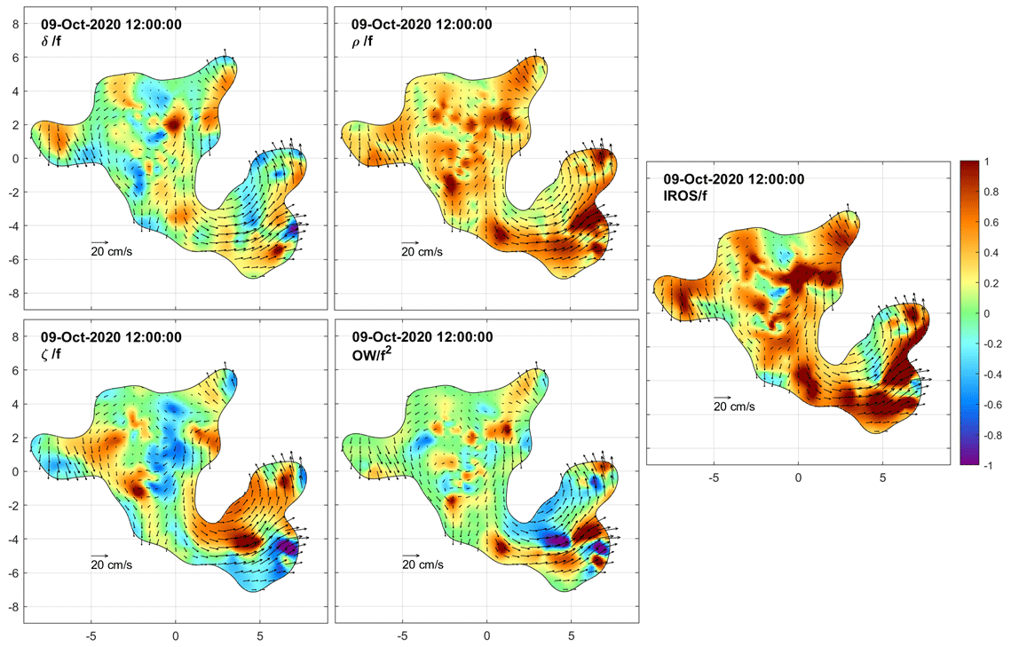
Figure 12 Same as Fig. 8 but for 9 October 2020 at 12:00 UTC.

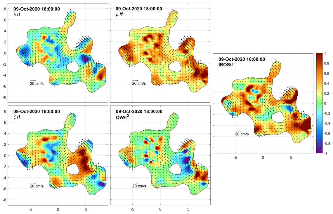
Figure 13 Same as Fig. 8 but for 9 October 2020 at 18:00 UTC.

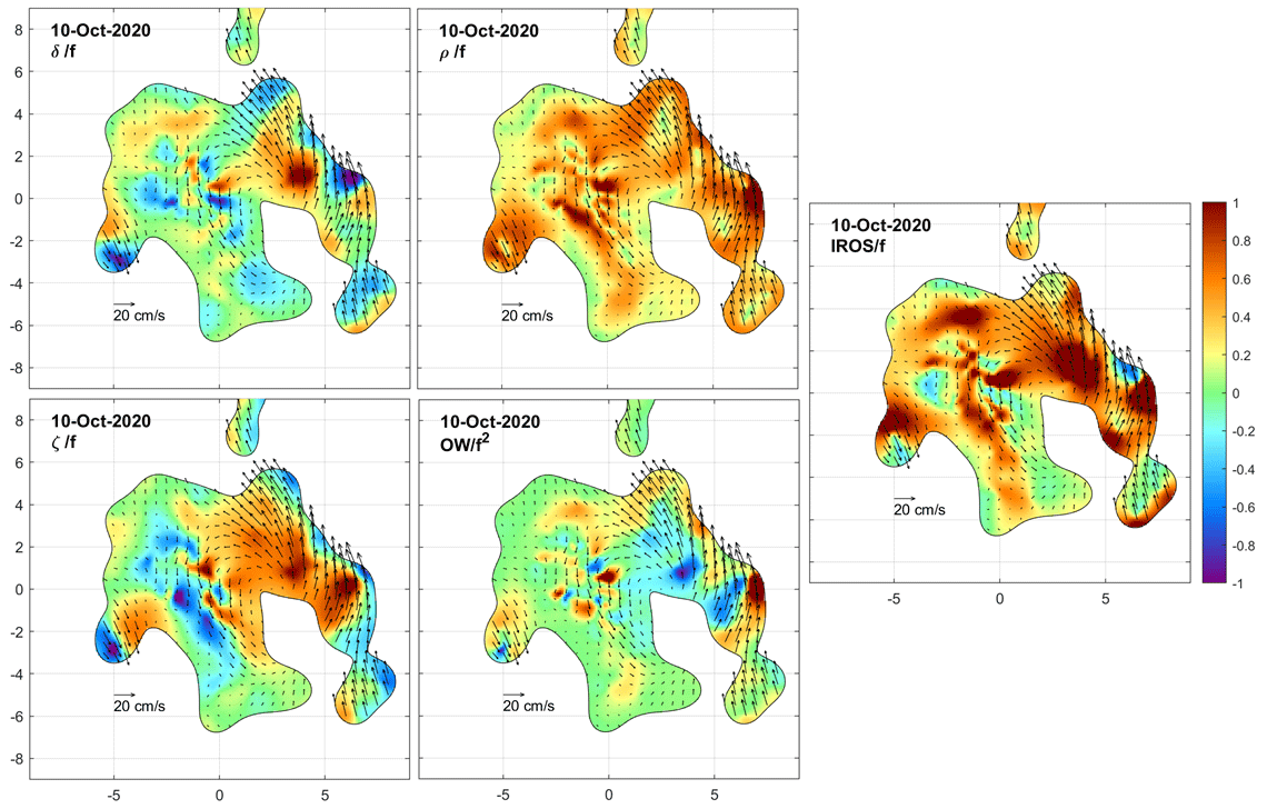
Figure 14 Same as Fig. 8 but for 10 October 2020 at 00:00 UTC.

On 10 October at 06:00 UTC, a few hours before the recovery operations (Fig. 15), a few drifters completed a full cyclonic loop in the eddy, now sampled more uniformly in all sectors.

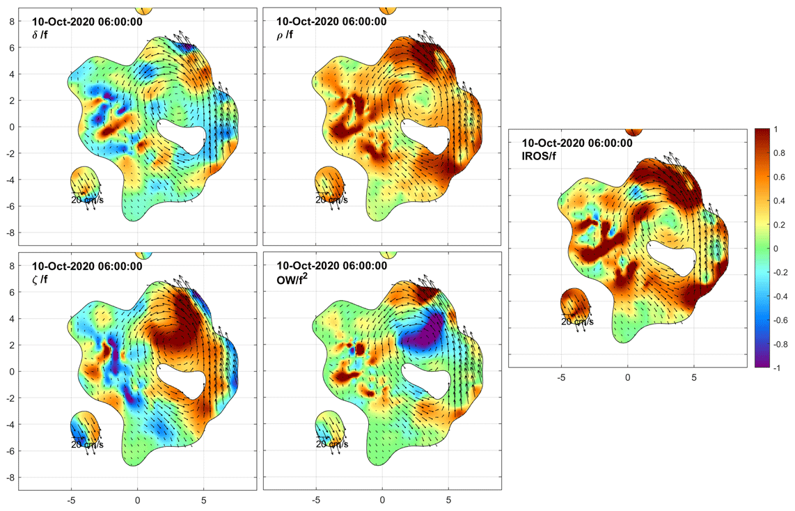
Figure 15 Same as Fig. 8 but for 10 October 2020 at 06:00 UTC.

As expected, the OW in the maps of Figs. 11–15 is always negative in the eddy core, corresponding to elliptic flow, while outside the eddy, the flow is hyperbolic and dominated by strain and deformation (positive OW). The horizontal divergence is essentially zero near the center of the eddy.

4 Discussion and conclusions

A small cluster (scale ∼ 6 km) of numerous Lagrangian instruments (more than 100 drifters and 1 profiling float) were deployed in the SLS coastal area on 8 October 2020 to characterize the near-surface submesoscale circulation and relative lateral dispersion. The instruments were tracked for about 2 d, and some of them were recovered on 10 October. During this period, the drifters were trapped in an offshore-flowing filament and a small cyclonic eddy. Satellite imagery of ocean color (near-surface chlorophyll concentration) revealed the shape of the filament extending tens of kilometers offshore in the southwestward direction and its evolution over time into a mushroom-like feature with small eddies developing at its southern and northern ends (Figs. 1 and 3). The speed of the near-surface currents measured by the drifters varied between 0 and 50 cm s⁻¹. The cluster moved toward the southeast at a mean speed of 10–20 cm s⁻¹ (Fig. 8). In 1 d, the cluster almost tripled in size (from ∼ 6 to ∼ 17 km).

Drifter velocities were used to estimate the DKPs and the relative dispersion of the near-surface currents on scales as small as 100 m. The DKPs within the cluster exhibit significant spatial and temporal variability, with absolute values reaching the order of magnitude of the local inertial frequency. Significant convergence was observed in the southwestward flow of the filament. A divergence of the order of f may correspond to significant vertical velocities in the upper mixed layer (Essink et al., 2019; Lodise et al., 2020; Tarry et al., 2021), leading to significant 3D dispersion of near-surface tracers (contaminants, biological organisms, etc.). Unfortunately, due the small number of SVP drifters drogued at 15 m, it is not possible to estimate vertical velocity in the study area. However, an approximate estimate of divergence at 15 m depth, based on the area rate of change method (Molinari and Kirwan, 1975) applied to the sparse coverage of independent SVP drifter triplets within the size range 2–7 km and with an aspect ratio larger than 0.2 (Esposito et al., 2021), shows an average value of 0.2 f, which is weaker than the magnitude found at the sea surface. Vorticity dominates in the core of the cyclonic eddy, where horizontal divergence is negligible. Strain prevails at the outer edge of the eddy. The Okubo–Weiss parameter shows areas of elliptic flow (OW < 0) in the eddy and hyperbolic flow (OW > 0) outside.

The relative dispersion on small scales (∼ 100–300 m) is initially exponential and related to some of the DKPs (e.g., instantaneous separation rate, strain and divergence; Figs. 6 and 7). After 5–10 h, or for initial separations greater than 500 m, the MSSD and FSLE show smaller relative dispersion rates with a slight decrease as a function of scale. The slope of the FSLE appears to be less than Richardson's $-\mathrm{2}/\mathrm{3}$ power law. This is expected since this theoretical law generally applies to scales larger than 10 km (Corrado et al., 2017; Lumpkin and Elipot, 2010; Bouzaiene et al., 2020), and in our study, the maximum separation scale is 7 km. Similarly to Schroeder et al. (2012), maximum FSLE values between 1 and 10 d⁻¹ for scales smaller than 300 m confirm that submesoscale dispersion is much larger in the coastal zone than in the open Mediterranean Sea (Lacorata et al., 2001; D'Ovidio et al., 2009) and open ocean (Corrado et al., 2017; Essink et al., 2019; Lumpkin and Elipot, 2010). In general, direct comparison of our dispersion results with the slopes predicted by two-dimensional geophysical turbulence theory is not satisfactory. This is not surprising since dispersion is due to advection by deterministic velocity fields that are highly variable in time and space, and the integration time of ∼ 2 d is not sufficient to consider dispersion as a random process. Deploying more drifters with smaller separation distances (tens of meters) and tracking them over a longer period (weeks) should provide more robust results that may be more comparable to the theoretical laws. However, the vicinity of the coastline might reduce dispersion rates.

In general, offshore transport and dispersion of coastal waters are shown to be significant at the submesoscale (< 10 km), including fast currents (up to 50 cm s⁻¹) that change rapidly (hours). Current operational numerical models for diagnosing or predicting coastal circulation (e.g., CMEMS; see Figs. 1 and 4) are not capable of simulating this variability and therefore are not yet suitable for investigating or predicting the complex coastal dynamics, particularly the advection and dispersion of tracers, such as biological constituents (e.g., chlorophyll) and contaminants. To achieve this goal, numerical models with higher spatial and temporal resolutions are needed, possibly nested in CMEMS simulations and driven by atmospheric models with similar resolution.