the Creative Commons Attribution 4.0 License.
the Creative Commons Attribution 4.0 License.
 | 25 Oct 2023
The Mediterranean Forecasting System – Part 1: Evolution and performance
Giovanni Coppini
Emanuela Clementi
Gianpiero Cossarini
Stefano Salon
Gerasimos Korres
Michalis Ravdas
Rita Lecci
Jenny Pistoia
Anna Chiara Goglio
Massimiliano Drudi
Alessandro Grandi
Ali Aydogdu
Romain Escudier
Andrea Cipollone
Vladyslav Lyubartsev
Antonio Mariani
Sergio Cretì
Francesco Palermo
Matteo Scuro
Simona Masina
Nadia Pinardi
Antonio Navarra
Damiano Delrosso
Anna Teruzzi
Valeria Di Biagio
Giorgio Bolzon
Laura Feudale
Gianluca Coidessa
Carolina Amadio
Alberto Brosich
Arnau Miró
Eva Alvarez
Paolo Lazzari
Cosimo Solidoro
Charikleia Oikonomou
Anna Zacharioudaki
The Mediterranean Forecasting System produces operational analyses and reanalyses and 10 d forecasts for many essential ocean variables (EOVs), from currents, temperature, salinity, and sea level to wind waves and pelagic biogeochemistry. The products are available at a horizontal resolution of ∘ (approximately 4 km) and with 141 unevenly spaced vertical levels.
The core of the Mediterranean Forecasting System is constituted by the physical (PHY), the biogeochemical (BIO), and the wave (WAV) components, consisting of both numerical models and data assimilation modules. The three components together constitute the so-called Mediterranean Monitoring and Forecasting Center (Med-MFC) of the Copernicus Marine Service.
Daily 10 d forecasts and analyses are produced by the PHY, BIO, and WAV operational systems, while reanalyses are produced every ∼ 3 years for the past 30 years and are extended (yearly). The modelling systems, their coupling strategy, and their evolutions are illustrated in detail. For the first time, the quality of the products is documented in terms of skill metrics evaluated over a common 3-year period (2018–2020), giving the first complete assessment of uncertainties for all the Mediterranean environmental variable analyses.
- Article
(9835 KB) - Full-text XML
-
Supplement
(365 KB) - BibTeX
- EndNote


Ocean analysis and forecasting systems are now available for the global ocean and regional seas at different spatial scales and with different numbers of essential ocean variables (EOVs) considered (Tonani et al., 2015). The societal drivers for the operational products that stem from the ocean analysis and forecasting products are the safety of maritime transport, multiple coastal hazards, and climate anomalies. Moreover, the operational products are at the basis of a new understanding of the dynamics of the ocean circulation (Pinardi et al., 2015); its linked biogeochemical cycles, namely carbon uptake and eutrophication, among others (Canu et al., 2015; von Schuckmann et al., 2020); and extreme storm surge events (Giesen et al., 2021).
The ocean analysis and forecasting system for the entire Mediterranean Sea was set up over the past 15 years (Pinardi and Coppini, 2010; Pinardi et al., 2017; Lazzari et al., 2010; Salon et al., 2019; Ravdas et al., 2018; Katsafados et al., 2016), and in 2015, it became operational in the framework of the Copernicus Marine Service, which is the marine component of the Copernicus Programme European Union service for sustainable use of the ocean, providing free, regular, and systematic information on the state of the blue (physical), white (sea ice), and green (biogeochemical) ocean on the global and regional scales. The Copernicus Marine Service in Europe has shown the strength of a state-of-the-art operational service implemented by hundreds of experts and teams who are distributed throughout Europe and come from public and private sectors, from operational and research organizations, from different countries, and from diverse cultures and relations to the ocean (Le Traon et al., 2017; Alvarez Fanjul et al., 2022). In this paper, we give an overview of the core components of the system, i.e. the numerical models and the data assimilation modules that represent the eddy-resolving ocean general circulation, the biogeochemical tracers, and the wind waves. Furthermore, we will document the quality of EOV products using goodness indices (Brassington, 2017). The core components constitute the so-called Mediterranean Monitoring and Forecasting Center (Med-MFC) of the Copernicus Marine Service (Le Traon et al., 2019). The integrated approach of the Med-MFC system represents a unique opportunity for the users to access state-of-the-art information provided in a uniform manner (e.g. same grid, unique format, and unique point of access). This ocean analysis and forecasting system, hereafter Med-MFC, produces analyses, 10 d forecasts, and reanalyses (Adani et al., 2011; Pinardi et al., 2015; von Schuckmann et al., 2016, 2018, 2019; Terzic et al., 2021; Simoncelli et al., 2016, 2019; Ravdas et al., 2018; Escudier et al., 2020, 2021; Cossarini et al., 2021).
An essential task of the production activities concerns the continuous assessment of the quality of the products (Sotillo et al., 2021; Alvarez Fanjul et al., 2022), which is achieved at two levels: (i) the pre-qualification of the systems before delivering a new release, including an extensive scientific validation of the products, published in the QUality Information Documents (QUIDs) available on the Copernicus Marine Product Catalogue; (ii) the operational evaluation of the skill metrics during operations, made available through the Copernicus Marine Product Quality Dashboard website (https://pqd.mercator-ocean.fr, last access: 30 June 2023), as well as through the Mediterranean regional validation websites implemented at the level of the Med-MFC production units (PHY: https://medfs.cmcc.it/, last access: 30 June 2023; WAV: http://Med-MFC-wav.hcmr.gr/, last access: 30 June 2023; BIO: https://medeaf.ogs.it/nrt-validation, last access: 30 June 2023). All the delivered variables are thus validated with respect to satellite and in situ observations using Copernicus Marine observational datasets, as well as additional datasets, climatologies, or literature information when needed.
The Mediterranean Sea is a semi-enclosed basin with an anti-estuarine circulation corresponding to a 0.9 and 0.8 ± 0.06 Sv baroclinic inflow and outflow at the Strait of Gibraltar, positive energy inputs by the winds, and net buoyancy losses inducing a vigorous overturning circulation (Cessi et al., 2014; Pinardi et al., 2019). The basin-scale circulation is dominated by mesoscale and sub-mesoscale variability (Pinardi et al., 2015; Bergamasco and Malanotte-Rizzoli, 2010; Pinardi et al., 2006; Robinson et al., 2001; Ayoub et al., 1998), with the former being subdivided into semi-permanent and synoptic mesoscales with spatial scales larger than 4–6 times the local Rossby radius of deformation. The stratification is large during summer in the first 50 m, and during winter the water column is practically unstratified. The Mediterranean Sea is an oligotrophic basin (Siokou-Frangou et al., 2010) with a west-to-east decreasing productivity gradient (Lazzari et al., 2012) and relatively high primary productivity in open-ocean areas where winter mixing increases surface nutrients (Cossarini et al., 2019). The wave conditions are driven by the winter storminess, while summer is characterized by low significant wave height values and higher value scatter (Ravdas et al., 2018). The yearly mean wave period, as estimated from available wave buoys over the Mediterranean Sea, amounts to 3.82 s with typical deviations of 0.92 s, while the mean significant wave height is 0.82 m (1.28 m as estimated by satellite observations) with typical deviations of 0.67 m (0.77 m for satellite data).
In this paper, we describe the final setup of the Med-MFC core components for the period 2017–2020. The Med-MFC modelling systems share the same grid resolution (∘) and bathymetry and use the same atmospheric and river forcing fields. Moreover, daily mean fields evaluated by the physical model are used to force the wave component (surface currents) and the transport–biogeochemical model (temperature, salinity, horizontal and vertical velocities, sea level, and diffusivity). This allows several model parameterizations to be calibrated to obtain the best result in terms of the specific environmental variable considered by each component. In the Copernicus Marine Service, the approach of forcing waves and biogeochemistry models with information from the hydrodynamic models is used and represents a standard which is also applied for the other MFCs. Several MFCs also use the online coupling between physics and wave models and between physics and biogeochemical models. Furthermore, this weakly coupled system ensures an efficient development of the data assimilation modules connected to each numerical model module and specific input datasets. It is a distributed system that shares information with efficiency and effectiveness when and how it is required by relevant processes. Due to its rather unique structure and the quality of its products, the system described could be used as a basic standard for new systems to be developed.
The paper is organized as follows. Section 2 provides an overview of the technical specifications of the Med-MFC components, Sect. 3 describes the quality of the system for a reference period from 2018 to 2020 and the quality of the forcing, and Sect. 4 concludes the paper and presents future perspectives.
The structure of the Med-MFC core components is shown in Fig. 1: the physical component (PHY) is composed of the NEMO general circulation model (Madec and the NEMO system Team, 2019) coupled to the WaveWatch-III (WW3) wave model (Clementi et al., 2017a) and the ocean data assimilation OceanVar 3DVAR (Dobricic and Pinardi, 2008 and Storto et al., 2015); the biogeochemical component (BIO) is composed of the Biogeochemical Flux Model (BFM), the tracer transport OGS Transport Model (OGSTM), and a data assimilation scheme (Lazzari et al., 2012, 2016; Cossarini et al., 2015; Vichi et al., 2020), forced daily by the daily mean of the PHY component fields; the wave component (WAV) is composed of the wave model WAM (WAMDI Group, 1988) and its assimilation scheme, forced daily by the daily mean of the PHY component fields. Daily 10 d forecasts, as well as analyses and reanalyses, are produced with all PHY, BIO, and WAVE components, as described below.
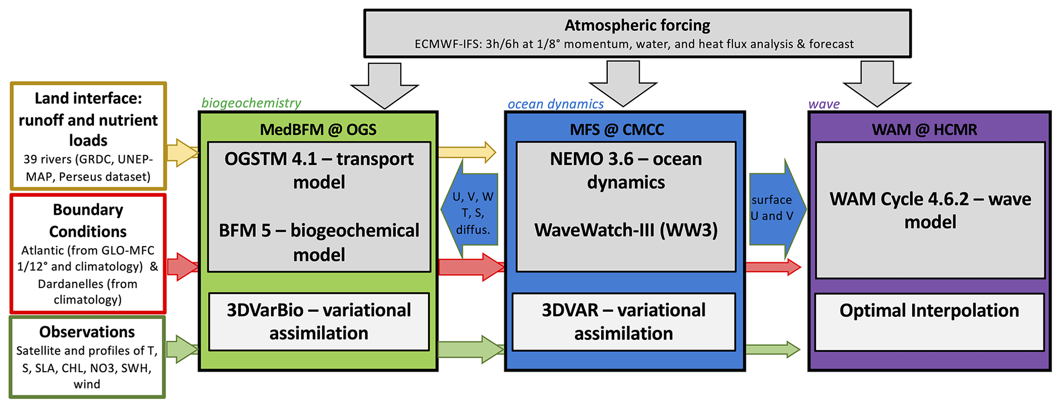
Figure 1The Med-MFC core components and the offline coupling scheme. The blue arrows are the exchanged fields at daily frequency between the three components.
Each component of the Med-MFC has its own data assimilation system; as such, an important effort was made to extract the most relevant information from satellite and in situ observations to produce the analysis and correct initial conditions for the forecast in order to benefit the forecasting skills. The main goal of the paper is to present the current quality of the operational system components by comparing the analysis and – for specific variables, such as significant wave height – the background (simulation) with in situ and/or satellite observations. The skill of the wave and biogeochemical models is assessed by considering intercomparisons of the model solution during the 24 h analysis phase with in situ and remotely sensed observations. As the latter are ingested into the model through data assimilation, the first-guess model fields (i.e. model background) are used instead of analyses.
2.1 The general circulation model component
2.1.1 Numerical model description
The PHY numerical model component comprises a two-way coupled current–wave model based on NEMO and WW3 implemented over the whole Mediterranean basin and extended into the Atlantic Sea in order to better resolve the exchanges with the Atlantic Ocean (Fig. 2). The model horizontal grid resolution is ∘ (ca. 4 km) and is resolved along 141 unevenly spaced vertical levels (Clementi et al., 2017b, 2019). The topography is an interpolation of the GEBCO (General Bathymetric Chart of the Oceans) 30 arcsec grid (Weatherall et al., 2015) that is filtered and specifically modified in critical areas such as the eastern Adriatic coastal areas (to avoid instabilities in circulation due to the presence of a large number of small islands), the Gibraltar and Messina straits (to better represent the transports), and the Atlantic edges external border (to avoid large bathymetric inconsistencies with respect to the Copernicus Global Analysis and Forecast product in which the model is nested). All the numerical model choices are documented in Table A1 in the Appendix.
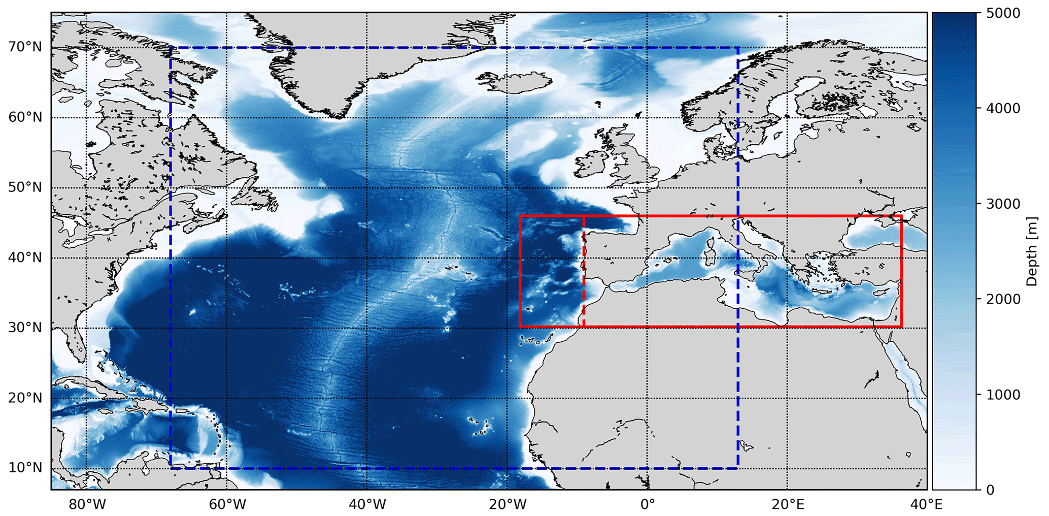
Figure 2The solid red box presents the domain of the PHY and WAV Mediterranean components. For BIO, the domain extends into the Atlantic as far as the dashed red line. The blue box presents one of the WAM domains, producing boundary conditions for the Mediterranean WAV component which extends only into the solid red box.
The general circulation model considers the nonlinear free-surface formulation and vertical z-star coordinates. The numerical scheme uses the time-splitting formulation to solve the free-surface and the barotropic equations with a (100 times) smaller time step with respect to the one used to evaluate the prognostic 3D variables (240 s). The active-tracer (temperature and salinity) advection scheme is a mixed upstream–MUSCL (monotonic upwind scheme for conservation laws; Levy et al., 2001) scheme, as modified in Oddo et al. (2009). The vertical diffusion and viscosity terms are defined as a function of the Richardson number following Pacanowski and Philander (1981). The air–sea surface fluxes of momentum, mass, and heat are computed using bulk formulae described in Pettenuzzo et al. (2010), and the Copernicus satellite gridded sea surface temperature (SST) data (Buongiorno Nardelli et al., 2013) are used to correct the non-solar heat flux using a relaxation constant of 110 W m−2 K−1 centred at midnight. A detailed description of other specific features of the model implementations can be found in Tonani et al. (2008) and Oddo et al. (2009, 2014).
The wave model WW3 is discretized by means of 24 directional bins (15∘ resolution) and 30 frequency bins (ranging between 0.05 and 0.7931 Hz) to represent the wave spectral distribution. The wave model is implemented using the same bathymetry and grid of the hydrodynamic model and uses the surface currents to evaluate the wave refraction but assumes no interactions with the ocean bottom. The Mediterranean implementation of WW3 follows WAM Cycle 4 model physics (Guenther et al., 1992); the wind input and dissipation terms are based on Janssen's quasi-linear theory for wind wave generation (Janssen, 1989, 1991), the wave dissipation term is based on Hasselmann's (1974) whitecapping theory according to Komen et al. (1984), and the nonlinear wave–wave interaction is modelled using the Discrete Interaction Approximation (DIA, Hasselmann et al., 1985). The exchanges between the circulation and wave models are performed using an online two-way coupling between NEMO and WW3. The models are forced by the same atmospheric fields (high-resolution ECMWF analysis and forecast winds) and are two-way coupled at hourly intervals, exchanging the following fields: NEMO sends to WW3 the sea surface currents and temperature, which are then used to evaluate the wave refraction and the wind speed stability parameter, respectively. The neutral drag coefficient computed by WW3 is passed to NEMO to compute the surface wind stress.
The NEMO–WW3 coupled system is intended to provide the representation of current–wave interaction processes in the ocean general circulation. At the moment, the feedback is considered only for the surface wind stress drag coefficient, and more details on this wave–current model coupling can be found in Clementi et al. (2017a).
2.1.2 Model initialization, external forcing, and boundary conditions
The PHY component was initialized in January 2015 using temperature and salinity winter climatological fields from WOA13 V2 (World Ocean Atlas 2013 V2, https://www.nodc.noaa.gov/OC5/woa13/woa13data.html, last access: 30 June 2023). The atmospheric forcing fields for both NEMO and WW3 models are from the ∘ horizontal resolution and 6 h temporal frequency (a 3 h frequency is used to force the first 3 d of forecasting) operational analysis fields from the European Centre for Medium-Range Weather Forecast (ECMWF) Integrated Forecasting System (IFS), and a higher spatial resolution of ∘ (with a higher forecast temporal frequency of 1–3–6 h according to the forecast leading time) is used starting from year 2020.
The circulation model's lateral open boundary conditions (LOBCs) in the Atlantic Ocean are provided by the Copernicus Global Analysis and Forecast product (Lellouche et al., 2018) at ∘ horizontal resolution and 50 vertical levels. Daily mean fields are used, and the numerical schemes applied at the open boundaries are the Flather (1976) radiation scheme for the barotropic velocity and the Orlanski (1976) radiation condition (normal projection of oblique radiation case) with adaptive nudging (Marchesiello et al., 2001) for the baroclinic velocity and the tracers. The nesting technique is detailed in Oddo et al. (2009), who also show a marked improvement in the salinity characteristics of the Modified Atlantic Water and in the Mediterranean sea level seasonal variability. The Dardanelles Strait boundary conditions (Delrosso, 2020) consist of a merge between the Copernicus global ocean products and daily climatology derived from a Marmara Sea box model (Maderich et al., 2015). The WW3 model implementation considers closed boundaries in both the Atlantic Ocean and the Dardanelles Strait.
The river runoff inputs consist of monthly climatological data for 39 major rivers (characterized by an average discharge larger than 50 m3 s−1) with a prescribed constant salinity at the river mouth (Delrosso, 2020) that is evaluated by means of sensitivity experiments and is listed in Table A4. More realistic and time-varying river salinity values (at least for major rivers) will be evaluated in future modelling evolutions using an estuary box model, such as the one presented in Verri et al. (2020), coupled to the hydrodynamic model.
2.1.3 The data assimilation component
A 3D variational data assimilation scheme, called OceanVar, initially developed by Dobricic and Pinardi (2008) and further improved for a wide range of ocean data assimilation applications (Storto et al., 2015), is coupled to NEMO.
The OceanVar scheme aims to minimize the cost function, as described in the following equation:
where ; x is the unknown ocean state, equal to the analysis xa at the minimum of J; xb is the background state; and is the misfit between an observation y and its modelled correspondent mapped onto the observation space to the observation location by the observation operator, H.
In OceanVar, the background error covariance matrix is considered to be B=VVT, where V is a sequence of linear operators: V=VηVHVV. Multivariate EOFs (empirical orthogonal functions, described in Dobricic et al., 2008 and Pistoia et al., 2017) compose the vertical component operator, VV. EOFs are computed in every grid point for the sea surface height, temperature, and salinity using a 3-year simulation in order to capture the mesoscale eddy variability that is assumed to represent the unbalanced component of the background error covariance. The horizontal covariances, VH, are modelled by an iterative recursive filter (Dobric and Pinardi, 2008; Storto et al., 2014). In order to assimilate altimeter observations, the dynamic height operator, Vη, developed in Storto et al. (2011), is used. A reference level of 1000 m is used for this operator so sea level anomaly (SLA) along-track observations over water shallower than this depth are not assimilated.
The observational error covariance matrix, R, is estimated following the relationship of Desroziers et al. (2005). The assimilated observations include along-track altimeter sea level anomaly from six satellites and in situ vertical temperature and salinity profiles from Argo floats. The SLA tracks provided by nadir altimeters are assimilated by subsampling every second observation to reduce the spatial correlation between consecutive measurements. A special quality control procedure is applied to real-time Argo data before they are assimilated. It consists of removing real-time profiles with negative temperature and/or salinity, temperatures higher than 45 ∘C, and salinities higher than 45 PSU; profiles with gaps in the observations of more than 40 m in the first 300 m depth (to avoid possible inconsistencies in the thermocline); and profiles with observations provided only below 35 m depth and observations in the first model layer (0–2 m). Moreover, a background quality check is implemented to reject observations whose square departure exceeds the sum of the observational and background error variances 64 times in the case of SLA and 25 times in the case of in situ temperature and salinity. The quality checks are applied to each individual observation of each Argo vertical profile and for each altimeter track. The misfits are computed at the observation time by applying the FGAT (First Guess at the Appropriate Time) procedure, and the corrections to the background are applied once a day to the restart file using observations within a 1 d time window.
2.2 The wind wave component
2.2.1 Numerical model description
The WAV component consists of two nested wave model implementations: the first grid covers the whole Mediterranean Sea at ∘ horizontal resolution, and it is nested within a coarser resolution wave model grid at ∘ horizontal resolution implemented over the Atlantic Ocean (Fig. 2).
The wave model is based on the state-of-the-art third-generation WAM Cycle 4.6.2, which is a modernized and improved version of the well-known and extensively used WAM Cycle 4 wave model (WAMDI Group, 1988; Komen et al., 1994). WAM solves the wave transport equation explicitly without any presumption regarding the shape of the wave spectrum. Its source terms include the wind input, whitecapping dissipation, nonlinear transfer, and bottom friction. The wind input term is adopted from Snyder et al. (1981). The whitecapping dissipation term is based on Hasselman's (1974) whitecapping theory. The wind input and whitecapping-dissipation source terms of the present cycle of the wave model are a further development based on Janssen's quasi-linear theory of wind wave generation (Janssen, 1989, 1991). The nonlinear transfer term is a parameterization of the exact nonlinear interactions (Komen et al., 1984; Hasselman et al., 1985). Lastly, the bottom-friction term is based on the empirical JONSWAP model of Hasselman et al. (1973).
The bathymetric map has been constructed using the GEBCO 30 arcsec bathymetric dataset for the Mediterranean Sea model and the ETOPO 2 dataset (US Department of Commerce, National Oceanic and Atmospheric Administration, NOAA National Centers for Environmental Information, 2022) 2 min gridded global relief data for the North Atlantic model. In both cases, mapping on the model grid was done using bi-linear interpolation accompanied by some degree of isotropic Laplacian smoothing. This bathymetry is different from the one used for the PHY component, optimized for the specific quality of the wave products.
The wave spectrum is discretized using 32 frequencies, which cover a logarithmically scaled frequency band from 0.04177 to 0.8018 Hz (covering wave periods ranging from approximately 1 to 24 s) at intervals of = 0.1 and 24 equally spaced directions (15∘ bin). The WAV model component runs in shallow-water mode considering wave refraction due to depth and currents in addition to depth-induced wave breaking. Modifications from default values of WAM 4.6.2 have been performed in the input source functions as a result of a tuning procedure. Specifically, the value of the wave age shift parameter (ZALP1 in the wind input source function was set to 0.011 (0.008 is the default) for the Mediterranean model, and the tunable whitecapping-dissipation coefficients CDS and δ were altered from their default values to become CDS=1.33 (2.1 default) and δ=0.5 (default value was 0.6). Finally, a limitation to the high-frequency part of the wave spectrum corresponding to the Cy43r1 ECMWF wave-forecasting system (ECMWF, 2016) was also implemented and tested in order to reduce the wave steepness at very high wind speeds.
2.2.2 Model initialization, external forcing, and boundary conditions
The WAV component is forced with 10 m above sea surface analysis and forecasted ECMWF winds at ∘ dissemination resolution. The temporal resolution is 6 h for the analysis, 3 h for the first 3 d of the forecast, and 6 h for the rest of the forecast cycle. From year 2021, a higher spatial (∘ for both analysis and forecast) and temporal (hourly for forecast days 1–3, 3-hourly for days 4–6, and 6-hourly for days 7–10) resolution dataset is used to force the WAV component. The wind is bi-linearly interpolated onto the model grids. Sea ice coverage fields used by the North Atlantic wave model are also obtained from ECMWF. With respect to current forcing, the WAV model is forced by daily averaged surface currents obtained from Copernicus Marine Service Med-MFC at ∘ resolution, and the North Atlantic model is forced by daily averaged surface currents obtained from the Copernicus global physical model at ∘ resolution. The WAV component runs one cycle per day, operating in analysis (for 24 h in the past (previous day)) and forecast (for 10 d in the future) modes. During the analysis phase, the model background is blended through data assimilation with available significant wave height (SWH) satellite observations at 3-hourly intervals and forced with ECMWF analysis 6-hourly winds and daily averaged surface currents.
The Mediterranean Sea model receives a full wave spectrum at 5 min intervals at its Atlantic Ocean open boundary from the WAM implementation in the North Atlantic. The latter model is considered to have all four of its boundaries closed, assuming no wave energy propagation from the adjacent seas. This assumption is readily justified for the north and west boundaries of the North Atlantic model considering the adjacent topography which restricts the development and propagation of swell into the model domain.
2.2.3 The wave data assimilation component
The assimilation module of the WAV component is based on the data assimilation scheme of WAM Cycle 4.6.2, which consists of an optimal interpolation (OI) of the along-track significant wave height (SWH) observations retrieved by altimetry and then a re-adjustment of the wave spectrum at each grid point accordingly. This assimilation approach was initially developed by Lionello et al. (1992) and consists of two steps. First, a best-guess (analysed) field of significant wave height is determined by OI with appropriate assumptions regarding the error covariance matrix. One of the key issues is the specification of the background error covariance matrix for the waves called P and the observation error covariance matrix, R. The first is defined as in the following equation:
while the second is defined according to Eq. (3) as follows:
where i and j are the model grid points in the longitudinal and latitudinal directions respectively, d is the distance of the observation location to the grid point, lc is the field correlation length, and and stand for the observation and model errors respectively. In the above expressions, the error is considered to be homogeneous and isotropic. We use R=1 and the correlation length lc equal to 3∘ (∼ 300 km).
Finally, the weights assigned to the observations are the elements of the gain matrix K, as presented in Eq. (4):
where H is the observation operator that projects the model solution to the observation location. For the current version of Med-waves, the OI analysis procedure is applied only to altimeter along-track SWH measurements, although wind at 10 m measurements can be assimilated as well. Prior to the OI procedure, quality-checked SWH observations which are available in a ±1.5 h time window are collocated with the closest model grid point and are averaged.
During the second step, the analysed significant wave height field is used to retrieve the full dimensional wave spectrum from a first-guess spectrum provided by the model itself, introducing additional assumptions to transform the information of a single wave height spectrum into separate corrections for the wind sea and swell components of the spectrum. Two-dimensional wave spectra are regarded either as wind sea spectra if the wind sea energy is larger than 3–4 times the total energy, or, if this condition is not satisfied, as swell. If the first-guess spectrum is mainly wind–sea, the spectrum is updated using empirical energy growth curves from the model. In the case of swell, the spectrum is updated assuming the average wave steepness provided by the first-guess spectrum is correct, but the wind is not updated.
Prior to assimilation, all altimeter SWH observations are subject to a quality control procedure. Every day, the system is scheduled to simulate 264 h: 24 h in the past (analysis) blending through data assimilation model results with all satellite SWH observations available followed by a 240 h forecast. The assimilation step adopted for the current version of the Med-waves system is equal to 3 h.
2.3 Mediterranean biogeochemical component
2.3.1 Numerical model description
The BIO component consists of the Biogeochemical Flux Model (BFM, Vichi et al., 2007) coupled with the transport (OGSTM) module (Salon et al., 2019). Advection, vertical and horizontal diffusion, and the sinking term for the biogeochemical tracers (Foujols et al., 2000) are solved by the OGSTM module that uses daily 3D velocity, diffusivities, and 2D atmospheric fields provided by the PHY component through the offline coupling scheme (Fig. 1). A source-splitting numerical time integration is used to couple advection and diffusion to the biochemical tracer rates.
BFM describes the biogeochemical cycles of carbon, nitrogen, phosphorus, silicon, and oxygen through the dissolved inorganic compartment and the particulate living and non-living organic compartments (Lazzari et al., 2012, 2016). The model includes four phytoplankton functional groups (i.e. diatoms, flagellates, picophytoplankton, and dinoflagellates), four zooplankton groups (i.e. carnivorous and omnivorous mesozooplankton, heterotrophic nanoflagellates, and microzooplankton) and heterotrophic bacteria. Among the nutrients, dissolved inorganic nitrogen is simulated in terms of nitrate and ammonia. The non-living dissolved organic compartment includes labile, semi-labile, and refractory organic matter. A carbonate system component (Cossarini et al., 2015) includes alkalinity (ALK), dissolved inorganic carbon (DIC), and particulate inorganic carbon (PIC) as prognostic variables; computes CO2 air–sea gas exchange according to Wanninkhof (2014); and provides diagnostics variables such as pH, CO2 concentration, and calcite saturation horizon.
2.3.2 Model initialization, external forcing, and boundary conditions
Initial conditions of nutrients (nitrate, ammonia, silicate, and phosphate), oxygen, and carbonate variables (DIC and alkalinity) consist of 16 climatological profiles homogeneously applied in each of the subregions represented in Fig. 3. Climatological profiles are computed from the European Marine Observation and Data Network (EMODnet) dataset (Buga et at., 2018). The other biogeochemical state variables (phytoplankton, zooplankton, and bacteria biomasses) are initialized in the photic layer (0–200 m) according to the standard BFM values. A 5-year hindcast is run using the first year (i.e. 2017) in perpetual mode. The model has two open lateral conditions: in the Atlantic Ocean and in the Dardanelles Strait. Nutrients, oxygen, DIC, and alkalinity in the Atlantic (i.e. boundary at long = 9∘ W) are provided through seasonally varying climatological profiles derived from the World Ocean Atlas (Boyer et al., 2018) and the literature (Alvarez et al., 2014), and a Newtonian dumping is applied. The Newtonian dumping is set between the longitudes 9∘ and 6.5∘ W with a timescale relaxation term linearly varying from 1/24 per day at 9∘ W to 90 per day at 6.5∘ W. A Dirichlet-type scheme with constant concentration values of nutrients, DIC, and alkalinity derived from the literature (Yalcin et al., 2017; Tugrul et al., 2002; Souvermezoglou et al., 2014; Copin-Montegut, 1993; Schneider et al., 2007; Krasakopoulou et al., 2017) is applied at the Dardanelles Strait. The concentrations are also tuned to provide input fluxes from the Black Sea to the Mediterranean Sea that are consistent with published estimates (Deliverable of Perseus, 2012; Yalcin et al., 2017; Tugrul et al., 2002; Copin-Montegut, 1993). A radiative condition is set for the other BFM tracers.
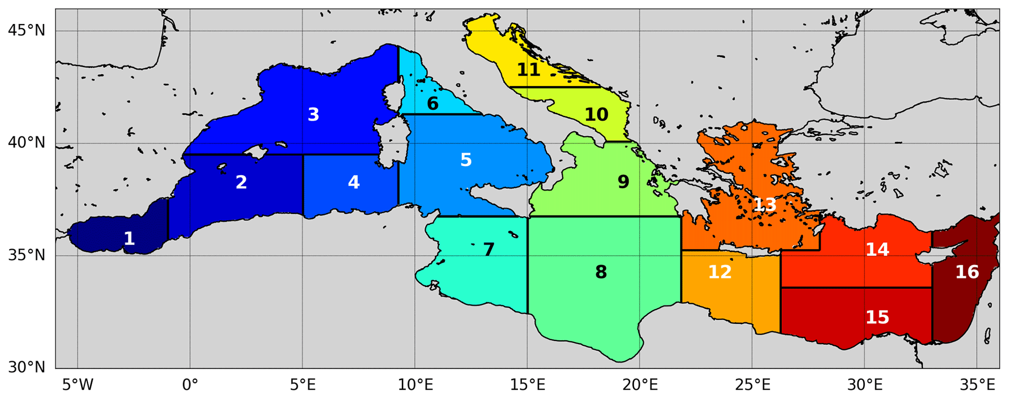
Figure 3The Mediterranean Sea domain and subregion subdivisions for analysis of the skill scores: Alboran (1), southwest Mediterranean-1 (2), northwest Mediterranean (3), southwest Mediterranean-2 (4), south Tyrrenian (5), north Tyrrenian (6), west Ionian (7), east Ionian (8), northeast Ionian (9), south Adriatic (10), north Adriatic (11), west Levantine (12), Aegean (13), north central Levantine (14), south central Levantine (15), east Levantine (16).
Terrestrial inputs include 39 rivers, consistent with the PHY component. Annual nutrients input are about 46 500 × 106 molN yr−1 and 881 × 106 molP yr−1 (Salon et al., 2019). Carbon and alkalinity inputs are 9300 × 109 gC yr−1 and 800 × 109 mol yr−1 respectively. Estimates are derived considering typical concentrations per freshwater mass in macro-coastal areas of the Mediterranean Sea (Copin-Montegut, 1993; Meybeck and Ragu, 1995; Kempe et al., 1991) and the river water discharges from the Perseus dataset (Deliverable of Perseus, 2012, as before). Annual atmospheric nutrient depositions are 81 300 × 106 molN yr−1 and 1194 × 106 molP yr−1 for nitrogen and phosphorus respectively (Ribera d'Alcalà et al., 2003). Spatially constant values of atmospheric pCO2 are derived from the 1992–2018 time series of the ENEA Lampedusa station (Trisolino et al., 2021), with the 2019 and 2020 values extrapolated by linear trend.
2.3.3 The biogeochemical data assimilation component
The BIO component features a variational data assimilation scheme (3DVarBio) which is based on the minimization of the cost function (Eq. 1) (Teruzzi et al., 2014). Minimization is computed iteratively in a reduced space using an efficient parallel PETSc/TAO (Portable, Extensible Toolkit for Scientific Computation and the Toolkit for Advanced Observation) solver (Teruzzi et al., 2019), and the background error covariance matrix, B, is factored as B=VVT, where V is a sequence of linear operators: V=VBVHVV. The horizontal error covariance operator (VH) is a Gaussian filter and includes a non-uniform and direction-dependent length-scale correlation radius to account for anisotropic coastal assimilation (Terruzzi et al., 2018) and vertical profile assimilation (Cossarini et al., 2019). The vertical error covariance operator (VV) is based on a set of 0–200 m vertical error profiles obtained using an empirical orthogonal function (EOF) decomposition of a 20-year-long pre-existing biogeochemical simulation. EOFs are computed monthly for the 16 subregions with the actual vertical resolution and are rescaled at each grid point considering the ratio between observation and model variances (Teruzzi et al., 2018). The biogeochemical error covariance operator (VB) is designed to preserve the ratios among phytoplankton functional types and their internal carbon-to-nutrient quotas (Teruzzi et al., 2014) and supports monthly and spatially varying covariances between dissolved inorganic nutrients (Teruzzi et al., 2021). In the most recent BIO model configuration (Teruzzi et al., 2021; Cossarini et al., 2019), the assimilated biogeochemical observations are satellite multi-sensor (MODIS, VIIRS (Visible Infrared Imaging Radiometer Suite), and OLCI – Ocean and Land Colour Imager) surface chlorophyll data (Volpe et al., 2019) and quality-controlled BGC-Argo nitrate and chlorophyll profiles (Schmechtig et al., 2018; Johnson et al., 2018). Ocean colour data are interpolated from original 1 km resolution to the ∘ model resolution.
2.4 System evolutions
The Mediterranean has been the site of major forecasting research activities since the late nineties (Pinardi et al., 2003; Pinardi and Coppini, 2010). The changes and evolution of the MED-MFS components are presented in Table 1. Before 2008, only the PHY and BIO components were present. The PHY component was based on the Ocean Parallelise (OPA) code (Madec et al., 1998) with the highest available horizontal and vertical resolutions of ∘ (approx. 6.5 km) in the horizontal and 72 vertical levels, with closed lateral boundaries; only seven major rivers; and the implementation of a weekly 3D-VAR assimilation scheme (Dobricic et al., 2007), assimilating temperature and salinity vertical profiles, sea level anomaly (SLA), and track altimeter data. Moreover, a non-solar heat flux correction was imposed through a nudging for the whole day with sea surface temperature (SST) satellite gridded data.
A major upgrade of the PHY component was achieved in 2009 by implementing a version of the numerical model NEMOv3.1 that included LOBCs in the Atlantic Ocean (Oddo et al., 2009) and by moving to a daily assimilation cycle. The first exchanges with a wave model were implemented in 2010 when the PHY component was coupled hourly with WAM, receiving the surface drag coefficient to better represent the wind stress. In 2013, the whole operational modelling system was updated by implementing an upgraded two-way online coupled system based on NEMOv3.4 and WW3 (Clementi et al., 2017a), allowing for a more consistent exchange between the two models. The following year, the PHY general circulation module was improved by accounting for the effect of atmospheric pressure (in addition to wind and buoyancy fluxes) and an explicit linear free-surface formulation using a time-splitting scheme (Oddo et al., 2014), while the assimilation scheme was enhanced thanks to the assimilation of Tailored Altimetry Products for Assimilation Systems (TAPAS) SLA data, allowing for the application of specific corrections of the altimetric original signal (Dobricic et al., 2012).
The PHY component delivered in 2015 included the nesting in the Atlantic Ocean through daily analysis and forecast fields from the global system, while 1 year later, the assimilation scheme was enhanced by including the computation of monthly and grid point EOFs and vertical observational errors varying with depth.
Another major PHY component evolution was achieved in 2017 when the resolution of the operational system was increased to ∘ (approx. 4 km) horizontal resolution and 141 vertical levels using the z-star vertical coordinate system, a nonlinear free-surface formulation, and when the NEMOv3.6 version and 39 rivers were introduced. From the year 2019, the Dardanelles Strait inflow was set as a lateral open boundary condition (instead of as a river runoff climatological input), allowing for a daily update of the fluxes, and an improved nudging with the satellite sea surface temperature was included by correcting the heat fluxes only close to midnight.
The WAV component was developed and released for the first time in 2017 based on WAM Cycle 4.5.4, providing on a daily basis 5 d wave forecasts and simulations for the Mediterranean Sea at ∘ horizontal resolution (Ravdas et al., 2018) nested within a North Atlantic model at ∘ resolution and forced with ECMWF 10 m winds and PHY component surface currents. In March 2018, the system was upgraded by incorporating the data assimilation component to utilize available track SWH satellite observations from Sentinel-3A and Jason-3. In 2019, the wave model was upgraded to Cycle 4.6.2, and the durations of the forecasts were extended to 10 d. Additionally, a limitation to the high-frequency part of the wave spectrum was applied, while modifications from default values were introduced in the input source and dissipation functions: ZALP was set to 0.011, and CDS and δ became 1.33 and 0.5 respectively.
In 2009, the first pre-operational version of the BIO component featured early versions of the OGSTM transport model and the BFM model (Lazzari et al., 2010). The spatial resolution was ∘, which required a subsampling of the PHY component fields from the ∘ resolution. The Atlantic boundary was closed with a nudging term for nutrients, and the land nutrients input included the three major Mediterranean rivers (i.e. Po, Rhone, and Nile), and the Dardanelles was treated as a river. BFM used constant daily averaged irradiance to force photosynthesis (Lazzari et al., 2010).
Horizontal resolution aligned with the physical model in 2013 and was refined to ∘ in 2017. Full alignment between the PHY and BIO components in terms of the same horizontal and vertical resolutions, bathymetry, and boundaries (number and position of rivers) was introduced in 2018 and remained a standard that mitigated possible approximation errors related to the use of daily outputs of the eddy-resolving ocean general circulation model to force the transport of tracers (Salon et al., 2019). Additionally, nutrient and carbon land inputs from 39 rivers were introduced in 2017, and open boundary conditions were introduced in Dardanelles Strait in 2019 and in the Atlantic Ocean in 2020 (Salon et al., 2019).
Since 2008, three major improvements of the BFM model have been integrated: (i) the addition of the carbonate system to predict alkalinity, ocean acidity, and CO2 air–sea exchanges in 2016 (Cossarini et al., 2015); (ii) the revision of nutrient formulation of phytoplankton in 2018 (Lazzari et al., 2016); and (iii) in 2020, the introduction of the day–night cycle in the light-dependent formulation of phytoplankton (Salon et al., 2019) and of the novel light extinction coefficient (Terzic et al., 2021).
A major system evolution and quality improvement was achieved in 2013 with the inclusion of the assimilation of satellite chlorophyll through a variational scheme with prescribed background error covariance (Teruzzi et al., 2014). The assimilation method was improved in 2018 to include coastal components (i.e. non-uniform and direction-dependent horizontal covariance; Teruzzi et al., 2018) and in 2019 to integrate new observations (i.e. BGC-Argo float profiles), including a new parameterization for the vertical and biogeochemical background error covariance (Cossarini et al., 2019).
In terms of operational product delivery, the BIO component has produced daily 10 d forecasts and weekly 7 d analyses since 2020, fully aligned with the PHY component (Salon et al., 2019). Before that, the system produced 7 d analyses and a 7 d forecast once per week since 2013, while a second cycle of 7 d forecasts was added each week in 2015.
The evaluation of the quality of the Med-MFC is given here only for the analysis products, leaving the assessment of the forecast skill for future work. One overarching driver for the Med-MFC evolution is the continuous improvement of the numerical model and data assimilation modules with respect to a well-defined set of goodness indices established for all the European regional seas (Hernandez et al., 2009). Ocean model uncertainties emerge from sources of error relevant to the ocean state, including physics, biogeochemistry, and sea ice, as well as errors in the initial state and boundary conditions (i.e. atmospheric forcing and lateral open boundary conditions). Model uncertainties in ocean physics have a significant impact on all other system components, as in, for example, biogeochemistry and sea ice (Alvarez Fanjul et al., 2022). Our results describe the quality of the Med-MFC products, presenting the statistics and accuracy numbers based on a reference simulation produced to calibrate and validate the operational forecasting systems, whereas the analysis of model uncertainty sources is outlined in the discussion part with reference to previous specific publications.
3.1 PHY component skill
The skill of the physical component is assessed over a 3-year period from 2018 to 2020 (Clementi et al., 2019). The evaluation is done by means of estimated accuracy numbers (EANs), which consist of the root mean square difference (RMSD) and bias (model minus observations) of the daily mean of model outputs against satellite and in situ observations. EANs are evaluated using the daily mean of model estimates interpolated on the available observations for that day; this goodness score is somewhat approximated, especially at the surface where daily variability is large, but this is a score used by many forecasting systems (Ciliberti et al., 2022; Toledano et al., 2022; Sotillo et al., 2021; Nagy et al., 2020), and we will show it for reference purposes. We also use misfits, which are the differences between the model solutions and the observations at the observational time during the forward model integration, for this assessment. The misfits provide quasi-independent and more accurate skill assessment since they are calculated before the variational analysis and at the observational time.
Table 1Changes in the Mediterranean forecasting components since 2008.
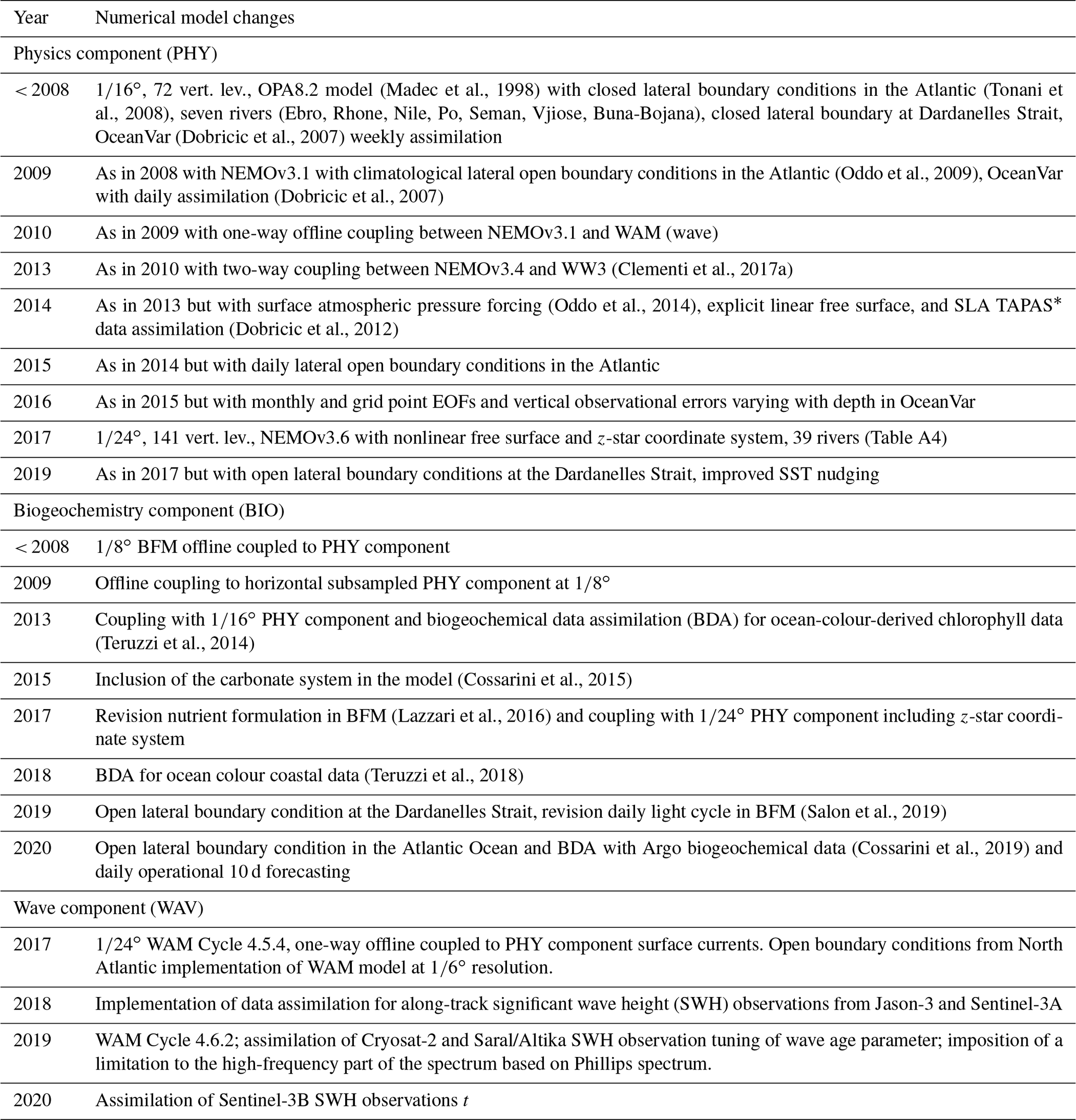
* The sea level anomaly (SLA) TAPAS product is produced to give information about the different corrections of the altimetric original signal.
Table 2EAN estimates with in situ observations. The differences (bias) and their squared values (RMSD) are then averaged over the whole Mediterranean Sea region and over nine vertical layers for the years 2018–2020.
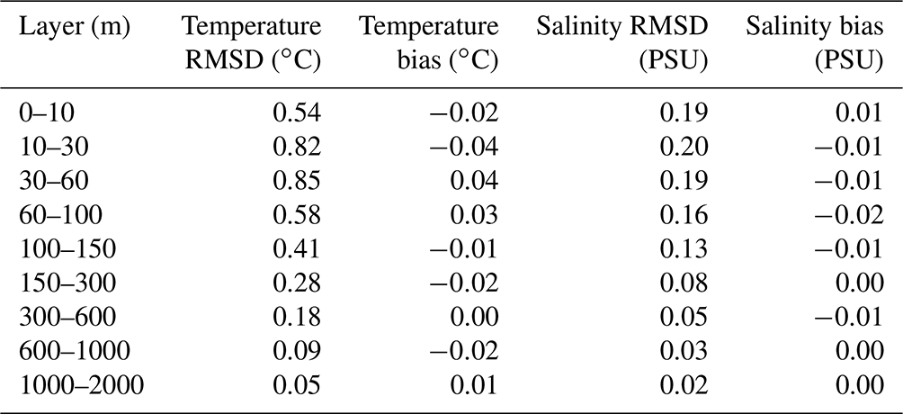
Table 2 summarizes the EAN of 3D model temperature and salinity daily mean values compared to in situ observations, in particular Argo floats and CTD profiles averaged over the 3 reference years. Model temperature shows small positive and negative biases depending on the depth, with the largest error (maximum value of the period is 0.85 ∘C) in the sub-surface layers between 10 and 60 m, decreasing with depth. Salinity is characterized by an almost generally negative small bias, meaning generally lower salinities than measured, along the whole water column except for the first layer. The salinity RMSD mean value is generally lower than 0.2 PSU, and the error is larger in the first layers and decreases significantly below 150 m. The comparison with other Copernicus Marine Service forecasting-system EAN values presented in the Quality Information Document (QUID), considering the fact that the validation periods are different, shows that the Mediterranean temperature and salinity qualities in terms of RMSD are aligned with all the other Copernicus forecasting systems. In particular, the average sea surface temperature RMSD with respect to satellite data ranges from 0.48 ∘C in the Northwest Shelf (derived from the QUID of the product NORTHWESTSHELF_ANALYSIS_FORECAST_PHY_004_013 https://doi.org/10.48670/moi-00054) to 0.8 ∘C in the Baltic Sea (derived from the QUID of the product BALTICSEA_ANALYSISFORECAST_PHY_003_006 https://doi.org/10.48670/moi-00010), while the 3D mean temperature RMSD with respect to in situ data ranges from 0.4 ∘C in the Mediterranean and Northwest Shelf to 0.7 ∘C in the Black Sea (derived from the QUID of the product BLKSEA ANALYSISFORECAST_PHY_007_001 https://doi.org/10.25423/cmcc/blksea_analysisforecast_phy_007_001_eas4), and the salinity mean RMSD varies from 0.1 PSU in the Mediterranean and Northwest Shelf to 0.3 PSU in the Iberia–Biscay–Ireland area (derived from the QUID of the product IBI_ANALYSISFORECAST_PHY_005_001 https://doi.org/10.48670/moi-00027). The sea level anomaly skill is also aligned with those of other operational systems within the Copernicus Marine Service when compared with satellite altimeter observations (from 2.2 cm in the Black Sea to 9 cm in the Northwest Shelf area).
The other goodness index is computed as weekly mean root mean square error and bias using temperature and salinity misfits that are computed at FGAT. The misfits are more precise in accounting for surface errors since the observations are compared with the model at the exact time of the day when observations are taken. This index is represented as a depth–time Hovmöller diagram in Fig. 4. The temperature error is seasonal (Fig. 4a), with maximum values of ∼ 1.8 ∘C in the range of 30–60 m depth, corresponding to the depth of the mixed layer and the seasonal thermocline during the stratified season from June to November. The error is reduced to an average value of around 0.4 ∘C during the vertically mixed season from December to May. The temperature misfits (Fig. 4c) indicate an overall overestimation of the temperature, except for in the subsurface layers, during winter and spring.
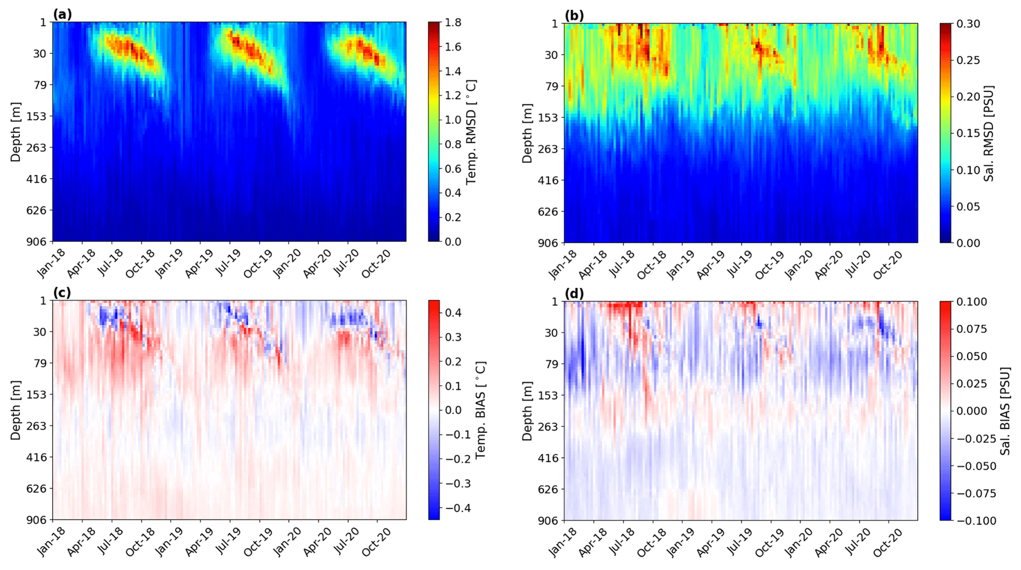
Figure 4Hovmöller (depth–time) diagrams: (a) weekly root mean square (rms) of temperature misfits, (b) weekly rms salinity misfits, (c) weekly bias of temperature, and (d) weekly bias of salinity evaluated along the water column and averaged over the whole Mediterranean Sea.
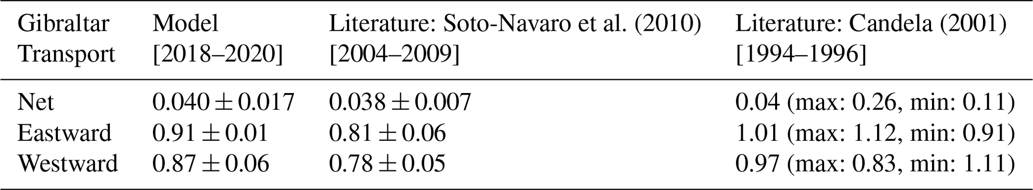
The salinity error (Fig. 4b) is defined by two main structures: one that is constant throughout the year down to about 150 m and the seasonal amplification during summer, as for the temperature errors. The maximum errors reach values of 0.35 PSU in the summer period and decrease to 0.025 PSU below ∼ 150 m. We argue that the background error, uniform throughout the year, could be due to inaccurate advection of salinity in different sub-areas of the Mediterranean Sea. Moreover, the model salinity bias is generally negative; i.e. the model salinity is lower than the observations (Fig. 4d). This could be related to the larger Atlantic water inflow with respect to the literature (Soto-Navaro et al., 2010) at Gibraltar, as reported in Table 3, and to inaccurate mixing at Gibraltar due to the lack of tides.
Table 3Gibraltar mean and standard deviation volume transports [Sv] from the Med-PHY numerical system averaged over the period 2018–2020 compared to literature values (current metre observations from October 2004 to January 2009).
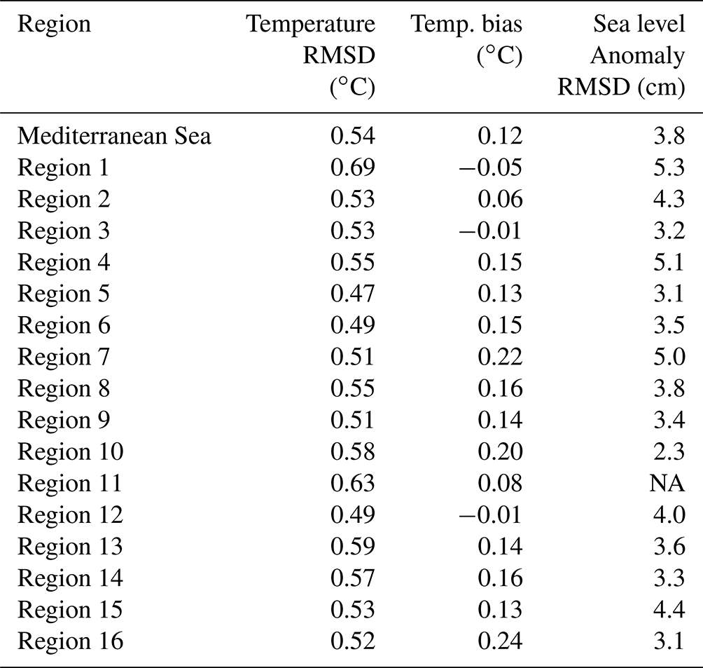
Sea surface temperature (SST) and sea level anomaly (SLA) skills are evaluated by comparing them with satellite observations: model daily mean SST is compared to SST satellite L4 gridded data at ∘ resolution (Buongiorno Nardelli et al., 2013), while SLA is compared to along-track satellite altimeter observations (Taburet et al., 2019) in terms of model misfits. Table 4 presents the RMSD and bias values computed for SST, as well as SLA RMSD averaged in the Mediterranean Sea and over the 16 subregions (see Fig. 3). Considering SST, the RMSD values range between 0.47 and 0.69 ∘C (mean Mediterranean Sea error is 0.54 ∘C), and the bias is generally positive, possibly caused by an overestimation of the downward shortwave radiation flux, which is estimated according to Reed's (1977) formula, as already discussed in Byun and Pinardi (2007) and Pettenuzzo et al. (2010). The SLA error ranges between 2.3 and 5.3 cm (mean error is 3.8 cm). The SLA skill scores vary in different regions; this could be related to the spatial coverage of the observations (not homogeneous in the basin) and to the limit of the 1000 m assimilation depth (due to the dynamic height operator, which assumes a level of no motion to compute the sea level increments from temperature and salinity increments; see Sect. 2.1.3).
Table 4EAN RMSD and bias of SST and SLA RMSD averaged over the whole of the Mediterranean Sea and the 16 subregions (see Fig. 3) for the period 2018–2020.
The time variability of the model SLA accuracy is also provided by means of weekly model misfits evaluated for each available satellite altimeter and averaged over the whole Mediterranean Sea, as shown in Fig. 5. The error ranges between 2.5 and 5.5 cm (maximum error with respect to CryoSat) with a large variability among the different satellites and with a generalized increase of error during autumn and winter seasons.
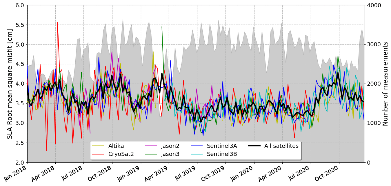
Figure 5Time Series of weekly mean rms misfit error for SLA evaluated with respect to available satellite altimeters and averaged over the whole Mediterranean Sea. The bold black line represents the mean error with respect to the whole set of satellites, which are separately shown with different colours. The grey area indicates the number of observations used for the validation.
3.2 WAV component skill
The quality of the wave analysis and forecast product is assessed over a 3-year period from January 2018 to December 2020. The skill of the Mediterranean wave model is assessed by considering intercomparisons of the model solution during the 24 h analysis phase with available in situ (SWH and mean wave period from wave buoys) and remotely sensed (SWH) observations. As the latter are ingested into the model through data assimilation, the model first-guess SWH (i.e. model background) is used instead of model analysis.
Significant wave height (SWH) and mean wave period (MWP) measurements are used for data validation from 28 wave buoys in the Mediterranean Sea (lower panel of Fig. 7). Data quality control procedures have been applied to the in situ observations (Copernicus Marine In Situ Team and Copernicus In Situ TAC, 2020), and measurements associated with a bad quality flag are not taken into consideration.
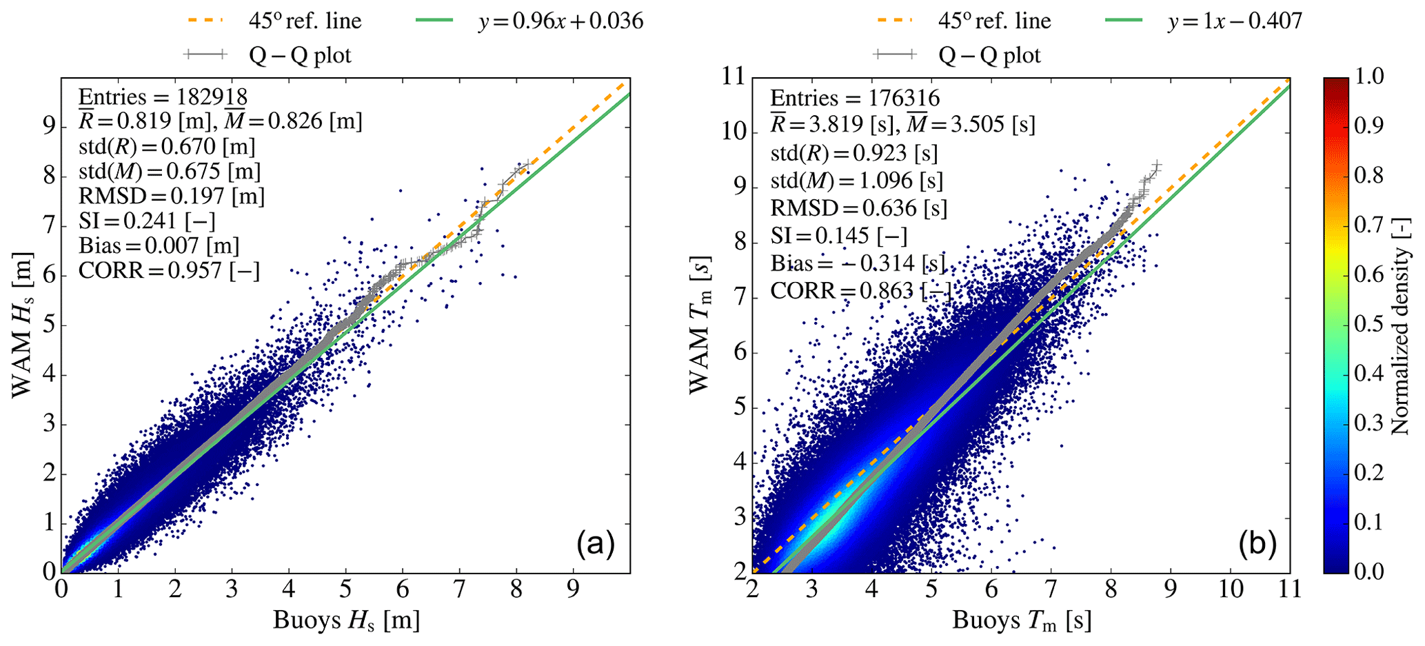
Figure 6Scatter plots of (a) significant wave height (Hs) and (b) mean wave period (Tm) versus wave buoy observations for the 28 stations of the Mediterranean Sea (Fig. 7c) for a 3-year period (2018–2020). The graphs also include quantile–quantile plots (grey crosses), 45∘ reference lines (dashed orange line), and least-squares best-fit lines (green line). At the top left of each picture, statistical scores are given: entries refer to the amount of data available for computing the statistics, R and M refer to the observed and modelled values respectively, SI is the scatter index (defined as the standard deviation of model–observation differences relative to the observed mean), and CORR is the Pearson correlation coefficient.
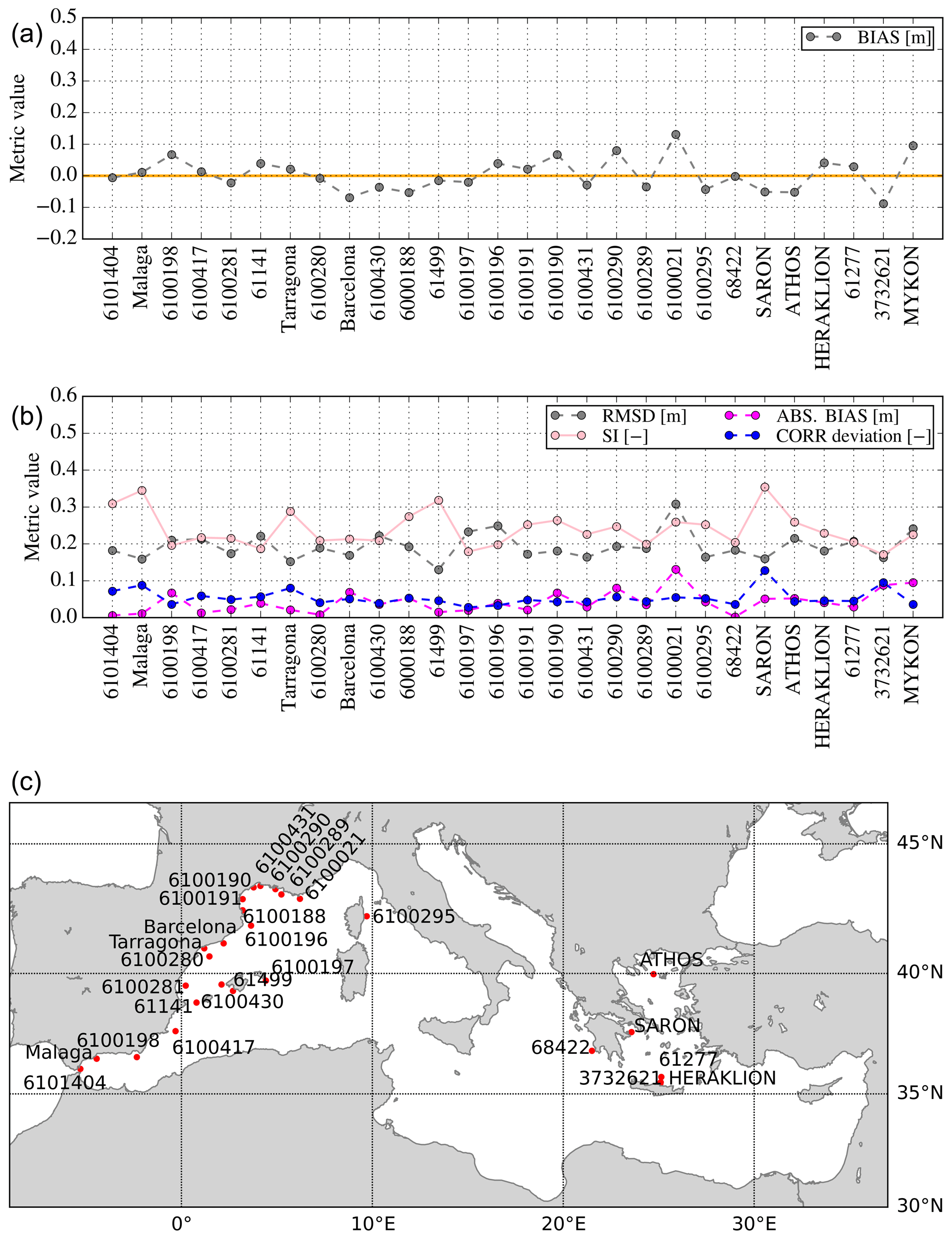
Figure 7Significant wave height difference between model and observations (a, b) at the 28 buoy locations (c) for a 3-year period (2018–2020). For all locations, the performance of the model is evaluated against buoy data by means of bias, root mean square difference (RMSD), scatter index (SI), and deviations of the Pearson correlation coefficient from unity (CORR deviation).
Figure 6 depicts scatter plots of the evaluation of the observed SWH and MWP against measurements obtained from the 28 buoys. For the immense amount of match-up data (within the range 0–1.25 m), the model overestimates SWH with respect to the buoy measurements (left side panel). Additionally, the model underestimates SWH during more energetic events (>1.25 m), except in the range 5.5–6.2 m. For large wave heights, model results underestimate SWH compared to the buoys, which agrees with past findings for the Mediterranean Sea (Ardhuin et al., 2007; Korres et al., 2011). Negative SWH bias can be attributed to errors in the forcing or inaccurate wave growth and dissipation at high wind speeds (Pineau-Guillou et al., 2018). The dashed orange line (i.e. the 45∘ reference line) in the quantile–quantile (Q–Q) plot stands for the unit gradient line. We observe that model results follow the dashed orange line very closely, meaning the model produces well the distribution of SWH observations. Although for higher waves (>1.25 m) the model tends to underestimate SWH (except in the range 5.5–6.2 m), it overproduces very large wave heights (100th, 99.97th, 99.96th, and 99.95th percentiles); hence, a deviation from the dashed orange reference line in the Q–Q plot becomes prominent for very high waves. Concerning MWP, the model systematically underestimates it (right side panel). Despite the overall modelled MWP underestimation (bias = −0.314 s), the system tends to overestimate MWP for high percentiles and/or very long waves (hence, we observe the deviation of the Q–Q plot from the unit gradient line for very high periods). Seasonal results (not shown) for both variables SWH and MWP indicated that the model adequately captures the seasonal variability. For SWH, RMSD values vary from 0.154 m in summer to 0.231 m in winter. Nevertheless, the scatter index (SI) is higher in summer (0.26) than during the other seasons. Additionally, the highest Pearson correlation coefficient (CORR) is observed in winter (0.963), while the lower one is equal to 0.932 and is observed in summer. The metrics reveal that the model better follows the observations in winter than during the other months since the former is associated with more well-defined weather patterns and higher waves. A similar conclusion has also been reached in other studies (e.g. Ardhuin et al., 2007) for the Mediterranean Sea. Summer and autumn are characterized by higher SI values (0.244 and 0.260 respectively), while lower values are obtained for winter and spring (0.231 and 0.227 respectively). Finally, small positive bias values are met for all seasons, with the highest values found in summer (0.012 m). Regarding mean wave period, RMSD varies from 0.610 s in summer to 0.66 s in winter, and bias is negative for all seasons. SI does not present significant seasonal variability, with the highest value encountered in summer. Finally, CORR for MWP is higher than 0.8 in all seasons (values are within the range 0.859–0.878, while during summer, CORR equals 0.792). These metrics demonstrate that the model wave period (similarly to the wave height) correctly follows the observations in well-defined weather conditions characterized by higher waves and longer periods, agreeing with past studies (Cavaleri and Sclavo, 2006; Ravdas et al., 2018).
The qualification metrics for the different buoy locations in Fig. 6 are plotted in Fig. 7 (upper panel). RMSD at the different buoy locations varies from 0.13 to 0.31 m. SI varies from 0.17 at buoy 3732621 to 0.35 at the buoys of Malaga and SARON (Aegean Sea). In general, SI values above the mean value for the whole Mediterranean Sea (0.24) are obtained at wave buoys located near the coast, particularly if these are sheltered by land masses to the north–northwest (e.g. western French coastline) and/or within enclosed basins characterized by a complex topography such as the Aegean Sea. As explained in several studies (Ravdas et al., 2018), in these cases, the spatial resolution of the wave model is often not adequate to resolve the fine bathymetric features, whilst the spatial resolution of the wind forcing is incapable of reproducing the fine orographic effects, introducing errors to the wave analysis. The Pearson correlation coefficient (CORR) mostly follows the pattern of variation of SI (in this figure, we present the CORR deviation from unity). CORR ranges from 0.87 at SARON in the Aegean Sea to 0.97 at the deep-water buoy 6100196 offshore Spain, which is well exposed to the prevailing northwesterly winds in the region. The bias varies from −0.13 m at buoy 3732621 (located north of Crete) to 0.13 m at buoy 6100021 located near the French coast. Its sign varies, with positive and negative values computed at almost the same number of locations respectively. Figure 8 (right) shows the scatter plot between the first-guess SWH and satellite observations. Here, the initial-guess SWH refers to the model SWH before data assimilation, thus meaning semi-independent model data. In addition, a scatter plot resulting from the comparison of the ECMWF forcing wind speeds (U10) and satellite measurements of U10 is shown in Fig. 8 (left). It is seen that ECMWF forcing overestimates U10 with respect to observations throughout most of U10 range, while some underestimation is observed for high wind speeds (14–19 m s−1). An overall ECMWF overestimation of 3 % is computed. On the other hand, the SWH model underestimation is about 6 %. Compared to the equivalent results obtained from the model–buoy comparison, a smaller scatter (by about 7 %) with a larger overall bias is associated with the model–satellite comparison, i.e. open-ocean waves. SI values compare well at the more exposed wave buoys in the Mediterranean Sea.
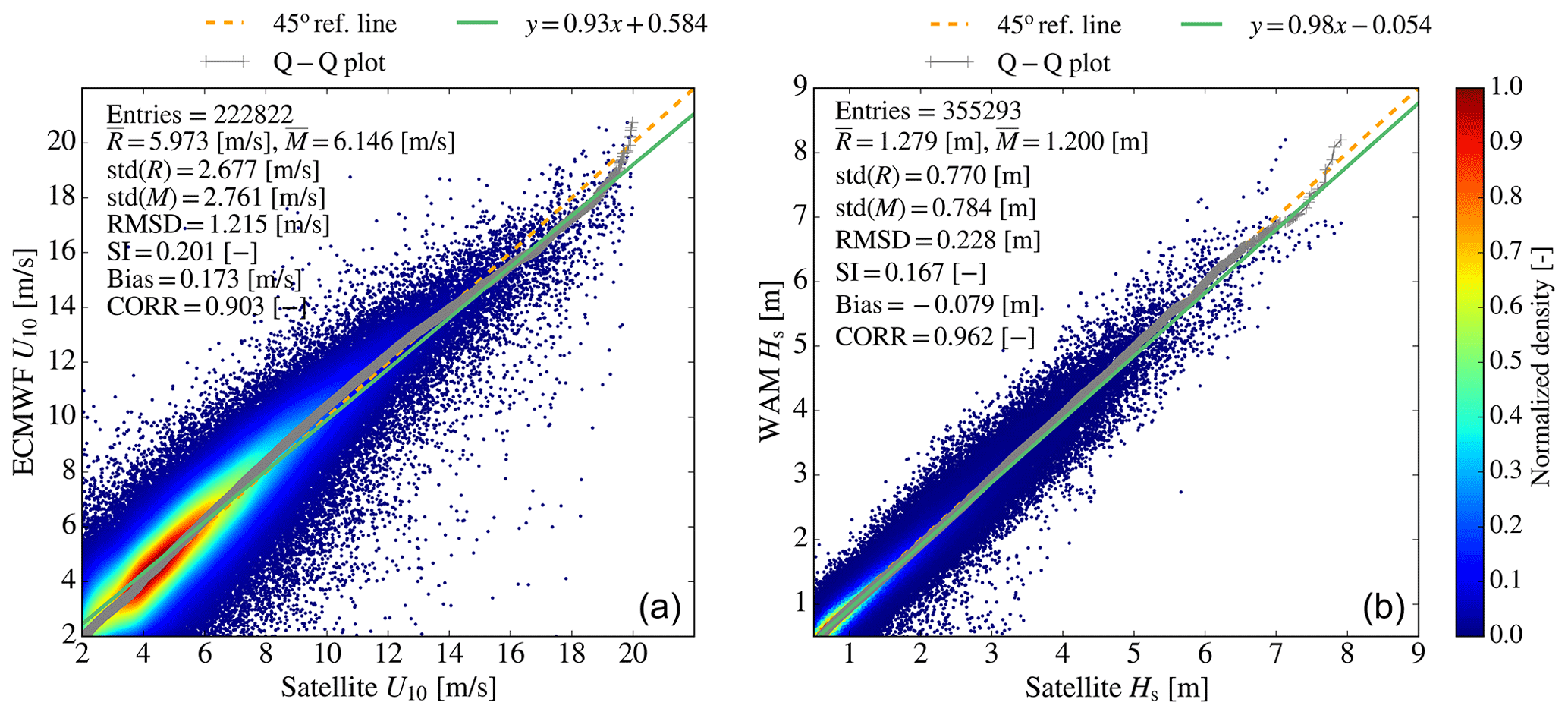
Figure 8Scatter plots of ECMWF forcing wind speed U10 versus satellite U10 observations (a) and model significant wave height (Hs) versus satellite observations (b) over the entire Mediterranean basin for the 3-year period (2018–2020).
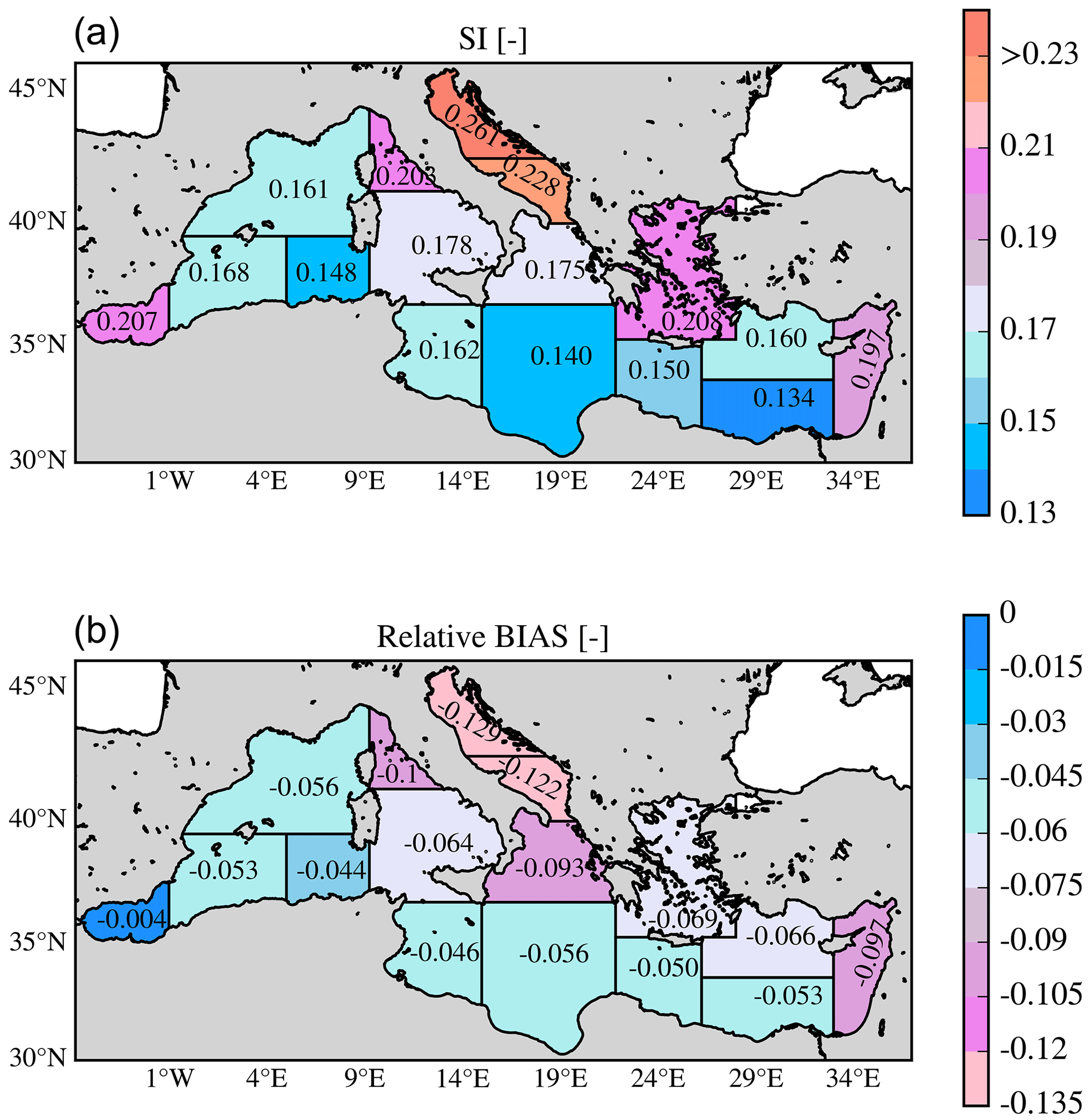
Figure 9SWH evaluation against satellite data: maps of scatter index (SI) (a) and relative bias (b) over the Mediterranean Sea subregions (shown in Fig. 3) for the 3-year period (2018–2020).
Figure 9 maps statistics of the comparison of model first guesses and satellite observations of SWH for the different subregions of the Mediterranean Sea. The Aegean and Alboran seas have relatively high SI values (0.21). The highest value of SI is obtained for the north Adriatic Sea (0.26) followed by the south Adriatic (0.23). The lowest values (0.13–0.15) are found in the Levantine Basin, the Ionian Sea, and the southwest Mediterranean Sea. Relatively low values (0.16) are also found west of the islands of Sardinia and Corsica. As discussed above, the error is due to inaccuracies associated with orographic winds and/or local sea breezes and the missing representation of the complicated bathymetry in the fetch-limited, enclosed regions. SWH negative bias is present in all subregions.
Finally, intercompared to ECMWF, UK Met Office, and DMI (Danish Meteorological Institute) wave forecasting systems for a different year (2014), Med-waves shows a better skill in terms of SWH, with RMSEs for the western Med buoys equal to 0.227 m (0.234 m for ECMWF and 0.281 m for UK Met Office) and 0.201 m for the central and eastern Mediterranean (0.227 m for ECMWF and 0.268 m for DMI).
3.3 BIO component skill
The BIO component state variables can be validated at three different uncertainty levels, providing degrees of confirmation (Oreskes et al., 1994) of different scales of variability based on the availability of reference data.
Near-real-time satellite and BGC-Argo float data provide a rigorous skill performance validation dataset down to the scales of the week and mesoscale dynamics for a limited set of variables: chlorophyll, nitrate, and oxygen. Datasets of historical oceanographic data (SOCAT dataset, Baker et al., 2016; EMODnet data collection, Buga et al., 2018; Cossarini et al., 2017; Lazzari et al., 2016) are used to build a reference framework of subregions and annual and seasonal climatological profiles to validate model performance to simulate the basin-wide gradients, the mean vertical profiles, and the seasonal cycle. For these datasets, it is possible to have nutrients such as nitrate, phosphate, ammonia, and silicate, as well as dissolved oxygen, dissolved inorganic carbon, alkalinity, and surface pCO2.
Lastly, a third level of validation regards those variables whose observability level is very scarce (e.g. phytoplankton biomass) or based on indirect estimations (e.g. primary production, air–sea CO2 fluxes). Only a confirmation of the range of variability and a general uncertainty estimation can be provided for those variables (see, for example, the validation of model primary production in von Schuckmann et al., 2020; Cossarini et al., 2020).
Considering the 2018–2020 reference period, the chlorophyll is very well reproduced by the BIO component, both in terms of seasonal cycle and spatial gradient at the surface (Fig. 10) and in terms of vertical profiles at the BGC-Argo float positions (Table 5). The uncertainty of the surface chlorophyll is lower than 0.03 mg m−3 with larger values registered in winter and western subregions where the variability and the chlorophyll values are higher (Fig. 10a and b). Regarding profiles, chlorophyll values and vertical shapes driven by mesoscale dynamics are simulated with a high level of accuracy by the model (Salon et al., 2019; Cossarini et al., 2019, 2021). Daily values of RMSD and of Pearson correlation are computed between satellite and model output maps and are then averaged over the two periods (Fig. 10c and d). The plot of RMDS (Fig. 10c) shows that higher errors are registered in the western subregions and in winter when chlorophyll levels and variability are higher. On the other hand, spatial correlation values are moderate and high in all subregions (i.e. values always above 0.5, except for a few subregions), with summer values being better than winter values. Considering the number of grid points in each subregion, all values in Fig. 10d should be considered to be significantly non-zero at the 0.05 level. Indeed, Salon et al. (2019) show how, using novel metrics, the BIO component reproduces with a high level of accuracy not only the concentrations in the euphotic layer but also the seasonal evolution of the shape of the profiles. The depth of the deep chlorophyll maximum during summer and of the surface bloom during winter, as well as the depth of the nitracline and the depth of the maximum oxygen layer, which result from the interaction of physical and biogeochemical processes, are reproduced with an uncertainty of O(101) m (Table 5). However, the conclusions about the mesoscale accuracy of the BIO component should be taken with caution since the BGC-Argo observations are still relatively few in number (about one-eighth of the Argo floats have biochemical sensors and are unevenly spaced (e.g. the southern Mediterranean Sea is less observed than northern areas).
Table 5The rms of the difference between MedBFM and Argo-BGC profiles for ecosystem metrics. RMSDs of the metrics are computed for each profile, then averaged over time and space considering the 2017–2020 period. Subregions: swm (reg2 + reg4), nwm (reg3), tyr (reg5 + reg6), adr (reg10 + reg11), ion (reg7 + reg8 + reg9), and lev (reg13 + reg14 + reg15 + reg16).
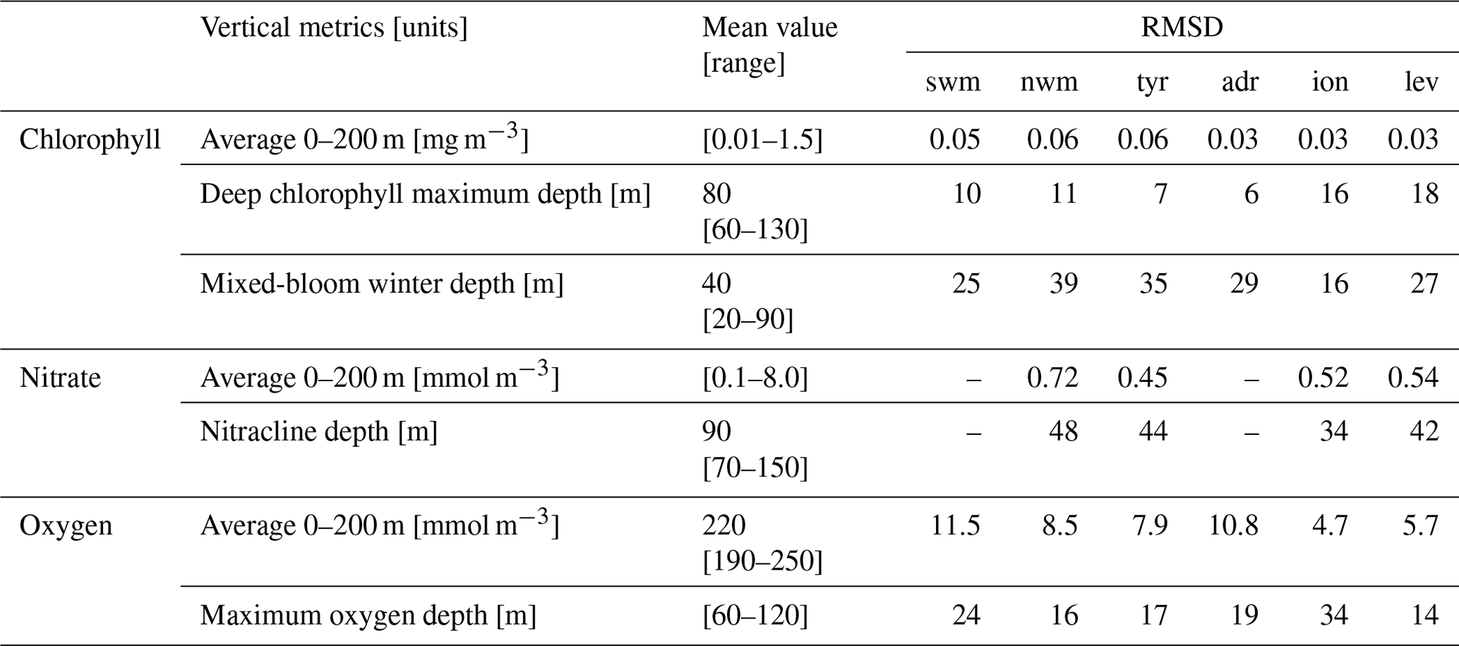
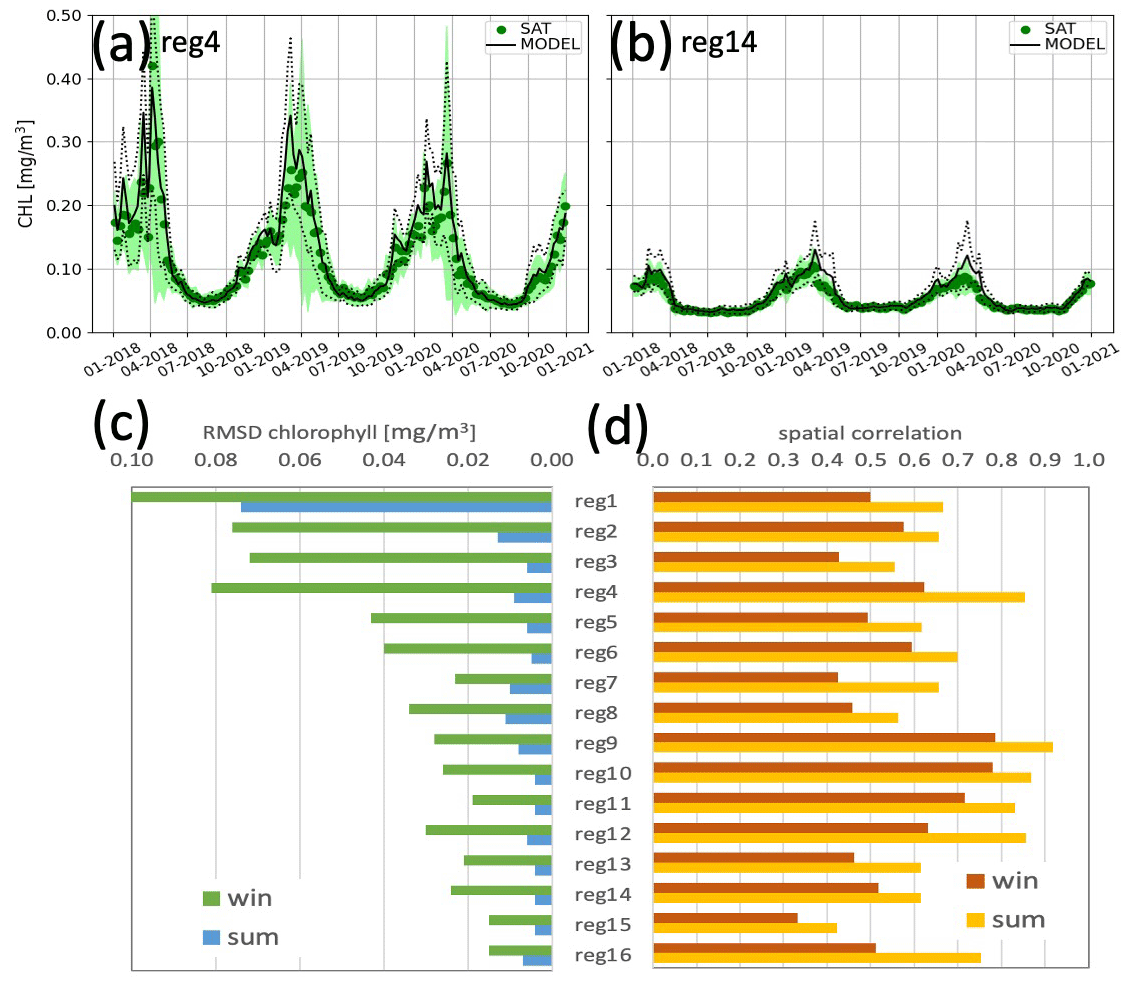
Figure 10Time series of surface chlorophyll for centred composite 7 d satellite analysis (green) and the model analysis (black) in two selected subregions (a, b). The rms of differences (c) and Pearson correlation (d) between maps of satellite and model forecast for the day before the assimilation in the 16 subregions of Fig. 5c. Metrics are averaged over the winter (from October to April) and summer (from May to September) periods.
As explained above, an additional verification of biogeochemical variables can be achieved for an additional seven variables (not considering chlorophyll) and two other derived variables with climatological data. An example of such a comparison is shown in Fig. 11 for the carbonate system variables. Average maps and profiles of alkalinity and DIC in selected subregions in the zonal directions (coloured lines) are superimposed well onto the range of variability in terms of the historical in situ data (grey-shaded areas), demonstrating the capability of the BIO component to reproduce both horizontal basin-wide gradients and vertical profiles in the different areas. A slight overestimation of DIC and alkalinity (underestimation of alkalinity) is simulated in the Alboran subregion in the upper 0–100 m layer.
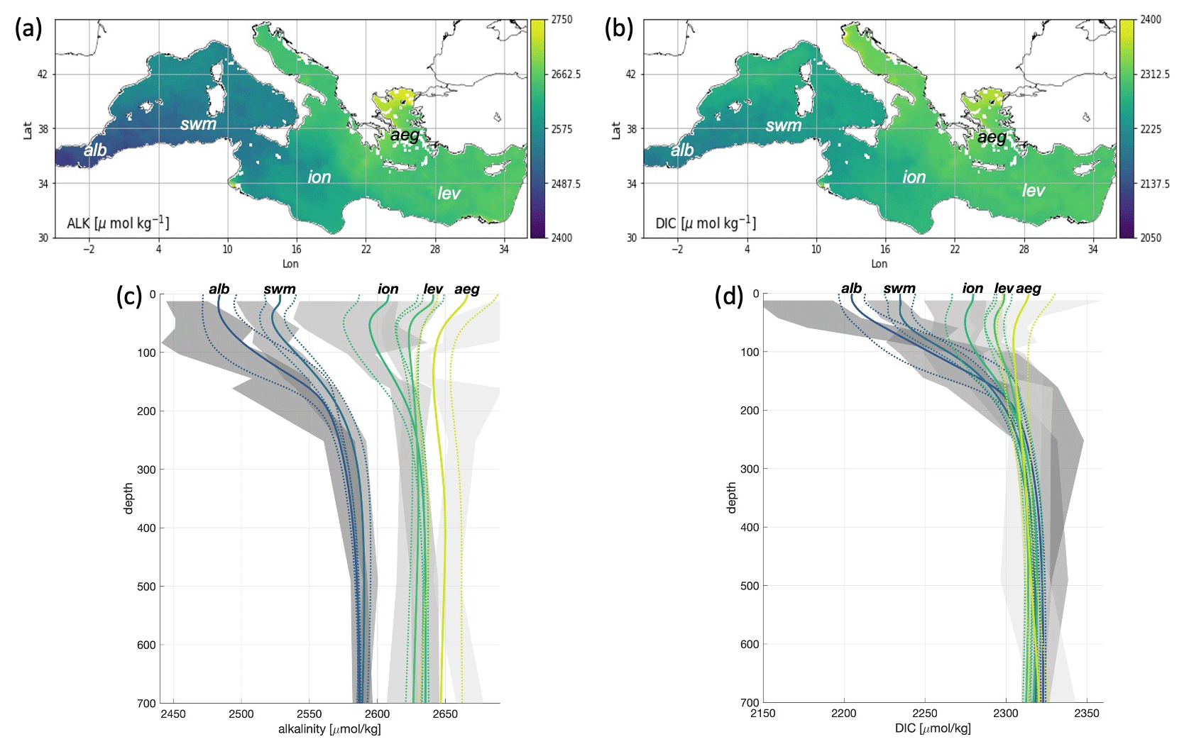
Figure 11Spatial distribution of modelled alkalinity (a) and DIC (b) and comparison of vertical profiles of alkalinity (c) and DIC (d) for model (average and range of variability represented by solid and dashed coloured lines respectively) and EMODnet climatology (average and range of variability represented black dots and lines and grey-shaded areas, respectively) for selected macro areas. Climatological data are computed using historical data (Buga et al., 2018; Bakker et al., 2014). The range of variability is the average ± standard deviation.
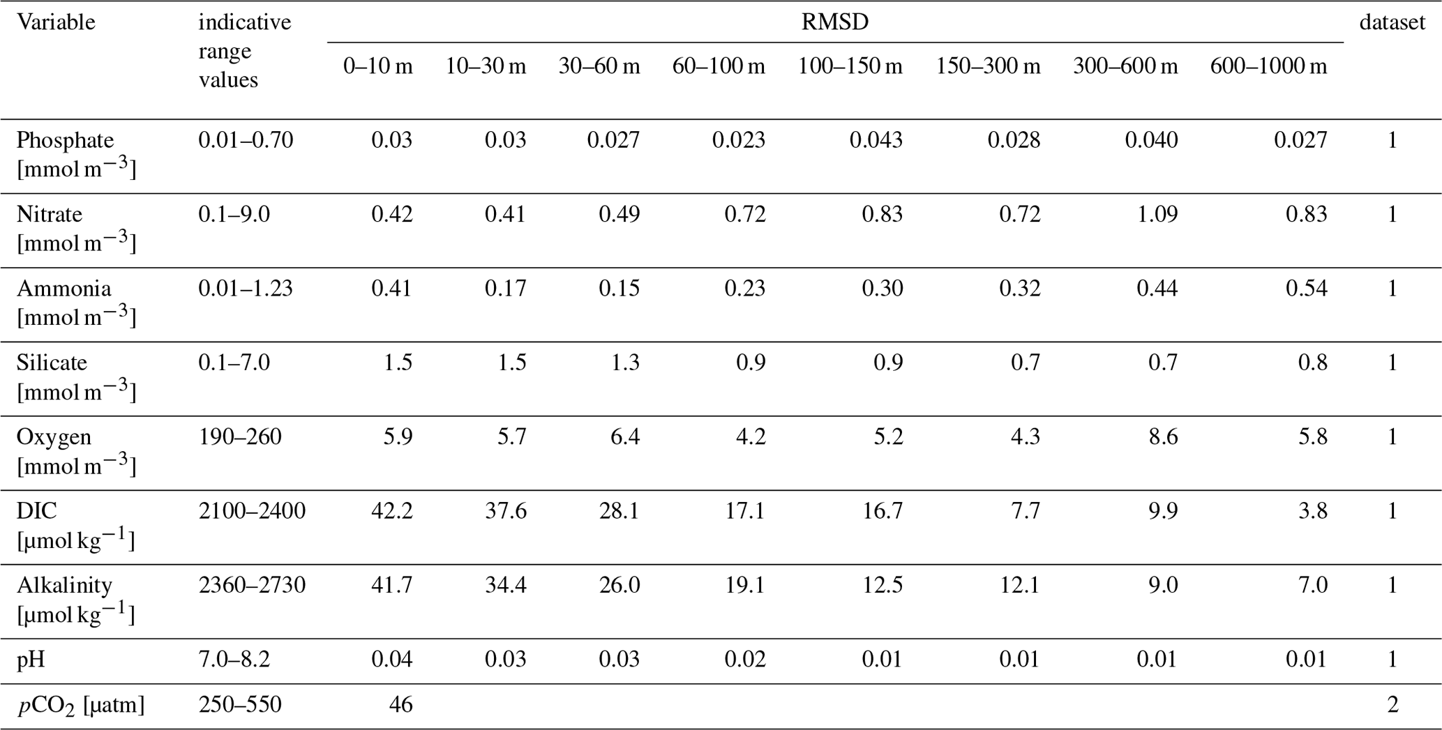
As a summary of the skill performance analysis, statistics based on RMSD for all the considered model variables (Table 6) report the model uncertainty in reproducing the basin-wide values and gradients for the selected layers. Generally, larger errors are computed for the upper layers where the variability (both spatial and temporal) is higher. Ammonia also indicates high errors in subsurface layers, which is due to a possible incorrect initialization of deep layers as a result of the lack of data in 9 out of 16 subregions. These numbers, which were found in response to the request for a synthetic measurement of the Copernicus Marine Service product accuracy (Hernandez et al., 2018), are consolidated by means of deep skill performance analysis of the BFM model in terms of reproducing chlorophyll (Lazzari et al., 2012; Teruzzi et al., 2018), nutrients (Lazzari et al., 2016; Salon et al., 2019), and carbonate system variables (Cossarini et al., 2015).
Table 6RMSD of the difference between model and climatological profiles at different depths evaluated in the 2017–2020 reference period. Statistics are computed using the 16 subregions in Fig. 3. Reference datasets for validation are: (1) EMODnet data collections (Buga et al., 2018) integrated with additional oceanographic cruises (Cossarini et al., 2015), and (2) Socat dataset (Bakker et al., 2014).
Chlorophyll from ocean colour is the most common variable used for validation and near-real-time assessment of operational biogeochemical models and allows for a comparison of the forecast skill performance among the Marine Copernicus systems. Results of surface chlorophyll skill scores show that the quality of the first day of the forecast of the BIO component is in line with that of other Copernicus models2 (Spruch et al., 2020; Vandenbulcke et al., 2021; McEwan et al., 2021; McGovern et al., 2020). In particular, the two proposed accuracy indexes (i.e. one minus scatter index and one minus the root mean square error normalized on variability) of the MED model equal to 34 % and 47 %, which are within the ranges of the other Copernicus systems: 11 %–38 % and 13 %–73 % for the two skill scores respectively (Spruch et al., 2020; Vandenbulcke et al., 2021; McEwan et al., 2021; McGovern et al., 2020).
For other biogeochemical variables, a direct comparison of the accuracy among Copernicus models is not straightforward, given the different protocols for metrics computation, the representativeness of the available observations, and the large range of variability of observed values of biogeochemical variables among the European seas. Nevertheless, a rough comparative assessment of the quality of Marine Copernicus biogeochemical models can be provided using published estimated EANs normalized by the typical values of the variables (McEwan et al., 2021; Feudale et al., 2021; Spruch et al., 2020; Melsom and Yumruktepe, 2021; McGovern et al., 2020; Vandenbulcke et al., 2021) to derive a common index of relative uncertainty. As for examples, the relative uncertainty of oxygen of the MED system is on the order of 2 %, which is in line with the other Copernicus systems, except for the Baltic and Black Sea systems, which show slightly higher relative errors. For nutrients, nitrate and phosphate uncertainties of the MED are about 50 % and 35 %, which are similar to or slightly better than most of the other Copernicus marine biogeochemical systems (i.e. ranges of 30 %–75 % and 30 %–50 % for nitrate and phosphate respectively). Finally, the relative uncertainty of pH simulated by the MED system is less than 0.5 %, while other Copernicus systems report relative errors on the order of 1 %–2 %.
Beside the aforementioned comparison, the MED biogeochemical system exhibits some distinguishable features: the continuous monitoring of the forecast skill of surface chlorophyll since the beginning of the operational biogeochemical system dating back to 2010 (Salon et al., 2019), a large number of validated variables with in situ data (i.e. up to 10 variables, Table 6), and the thorough use of BGC-Argo observations for near-real-time forecast validation (Salon et al., 2019; Cossarini et al., 2021; https://medeaf.ogs.it/nrt-validation, last access: August 2022).
3.4 ECMWF forcing skill
A calibration and validation system of the ECMWF forcing fields used by the Med-MFC operational systems has been developed using in situ ground meteorological observations from METeorological Aerodrome Report (METAR) stations and numerical model data from ECMWF (see Fig. 12). Four well-established statistical indices for validating 2 m temperature, dew point temperature, air pressure, and wind speed have been defined: (a) bias, (b) RMSE, (c) Nash–Sutcliffe model efficiency coefficient, and (d) correlation coefficient.
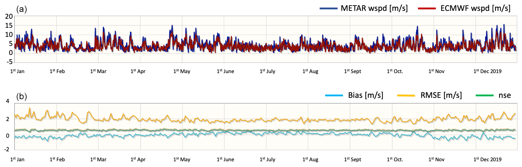
Figure 12Example of ECMWF wind speed validation with respect to METAR ground observations in 2019 in the area of the Gulf of Lion. (a) Time series of daily mean wind speed time series from METAR station (blue line) and from ECMWF (red line). (b) Time series of main skill metrics (bias, root mean square error (RMSE), and Nash–Sutcliffe model efficiency coefficient (nse)).
The atmospheric forcing calibration and validation system will become publicly available, and an example of this validation is provided in Fig. 12, showing daily mean wind speed time series from a METAR station (blue line) and ECMWF (red line) in the area of the Gulf of Lion during the year 2019, as well as time series of the main skill metrics.
In this paper, the Med-MFC components (PHY, BIO, and WAV) have been described, providing an overview of their technical specifications. The PHY component provides 3D currents, temperature, and salinity with the BIO and WAV components daily, with daily mean values. This model system is flexible enough that improvements can be carried out separately on the three components, considering the different levels of maturity of the numerical modelling parameterizations, the data assimilation components, and the validation datasets. A different data assimilation system is run for each component, making the best use of all available data from satellite and in situ observations; the effort is to assimilate as much data as possible and use background or model uncertainties to account for the missing couplings. The three components' accuracy has been evaluated for a common 3-year period, from January 2018 to December 2020.
The PHY component has been validated by comparing model data to in situ and satellite observations, showing good accuracy in representing the spatial pattern and the temporal variability of the temperature, salinity, and sea level in the Mediterranean Sea. In particular, the model has a warm surface temperature bias of +0.12 ∘C when compared to satellite SST. The water column temperature error has a clear seasonal signal with the largest errors at the depth of the surface mixed layer and the seasonal thermocline. The model error in salinity is higher in the first layers and decreases significantly below 150 m. The SLA presents a mean average error of 3.8 cm over the 3-year-averaged period for the whole basin.
The WAV component was extensively validated for the 3-year period using all available in situ and satellite observations in the Mediterranean Sea. All statistical values calculated and presented here showed a very good system performance. It is concluded that the Mediterranean SWH is accurately simulated by the WAV component. The typical SWH difference with observations (RMSE) over the whole basin is 0.21 m (0.197 m for in situ and 0.228 m for satellite observations) with a bias ranging from −0.137 to −0.005 m when the comparison is against the in situ observations and from to −0.088 to 0.131 m when the comparison is with satellites. The scatter index (SI) exhibits low values (0.13–0.17) over the majority of the basin and relatively higher values (0.18–0.21) over the Aegean, Alboran, Ligurian, and east Levantine seas, with the highest SI value encountered in the north Adriatic Sea (0.26). As explained, the occurrence of higher SI values is mainly related to the quality of ECMWF winds in fetch-limited areas of the basin where the orographic effects play an important role and to the difficulties of wave models in appropriately resolving complicated bathymetry and coastline.
Overall, the quality of the WAV component stems from the ECMWF wind forcing that drives the wave dynamics, data assimilation, forcing from Med-PHY surface currents, and improved parameterization of the wave wind source and dissipation terms of the WAM model. In particular, the WAV component assimilates satellite altimetry data with a well-calibrated stand-alone OI scheme and implements regular updates and improved parameterization independently from the other components. Given that wind-forcing quality has a substantial influence on the model response, a considerable part of the wave product uncertainty, especially under high winds or extreme conditions, is related to the wind-forcing uncertainty and can be substantially improved by undertaking the ensemble approach in wave forecasting. The lower accuracy of the wave product in semi-enclosed regions of the Mediterranean Sea (e.g. Adriatic and Aegean seas) can be related to the current spatiotemporal resolution of the wind forcing. Near the coast, unresolved topography by the wind and wave models and fetch limitations causes the wave model performance to deteriorate. In particular, the WAV component assimilates satellite altimetry data with a well-calibrated stand-alone OI scheme and implements regular updates and improved parameterization independently from the other components. Given that wind-forcing quality has a substantial influence on the model response, a considerable part of the wave product uncertainty, especially under high winds or extreme conditions, is related to the wind-forcing uncertainty and can be substantially improved by undertaking the ensemble approach in wave forecasting. The lower accuracy of the wave product in semi-enclosed regions of the Mediterranean Sea (e.g. Adriatic and Aegean seas) can be related to the current spatiotemporal resolution of the wind forcing. Near the coast, unresolved topography by the wind and wave models and fetch limitations cause the wave model performance to deteriorate.
The BIO system has defined a validation framework (Salon et al., 2019) based on multivariate (e.g. more than 10 variables) and multilevel metrics that include Global Ocean Data Assimilation Experiment (GODAE) class-1 and class-4 statistics and process-oriented metrics. Of particular interest is that the present validation framework also includes near-real-time observations (i.e. satellite and BGC-Argo) that show average errors in the 0–200 m layer of 0.04 mg m−3, 0.4 mmol m−3, and 16.8 mmol m−3 for chlorophyll, nitrate, and oxygen respectively. Thus, the validation framework represents a robust benchmark for the future improvements of the Mediterranean BIO model. Indeed, as detailed in Salon et al. (2019) and Cossarini et al. (2021), critical sources of the BIO model errors include unresolved Atlantic boundary conditions, as well as land–sea and atmosphere–sea forcing uncertainty in model parameterization and the inconsistency of coupled physical–biogeochemical processes.
The value and reliability of the Med-MFC systems are demonstrated by the several downscaling coastal model systems and downstream applications that use its outputs operationally. The CYCOFOS (Cyprus Coastal Ocean Forecasting and Observing System) (Zodiatis et al., 2003), which is a subregional forecasting and observing system in the eastern Mediterranean Levantine Basin, uses the Med-MFC outputs to set its boundary conditions. The Med-MFC outputs are used as initial and lateral boundary conditions by the physical and wave ocean system MIT Operational (MITO), which provides 5 d forecasts at a resolution up to ∘ (Napolitano et al., 2022). The Southern Adriatic Northern Ionian coastal Forecasting System (SANIFS) is a coastal–ocean operational system providing short-term forecasts since September 2014 (Federico et al., 2017). It is built on the unstructured-grid, finite-element, three-dimensional, hydrodynamic Shallow water HYdrodynamic Finite Element Model (SHYFEM) model and is based on a downscaling approach starting from the large-scale system Med-MFC, which provides the open-sea fields.
The CADEAU (Assimilation of national water quality data in Coastal Areas for a marine Directives oriEnted downstreAm prodUct) physical–biogeochemical forecasting system of the northern Adriatic Sea (Bruschi et al., 2021) is based on a high-resolution (up to 700 m) application of the MITgcm-BFM model (Cossarini et al., 2017), targeting water quality and eutrophication and using the daily Med-MFC products for initialization and to constrain the southern boundary.
In addition, the Gutta savinG fUel and emissions from mariTime Transport in the Adriatic region (GUTTA-VISIR) system, which can be defined as a tactical, global-optimization, single-objective, deterministic model system for ship route planning (Mannarini et al., 2016a, b; Mannarini and Carelli, 2019), uses the analysis and forecast wave and current fields from the Med-MFC in conjunction with wind fields from ECMWF.
Since 2008, the Med-MFC components have been continuously upgraded and substantially improved. The system evolution will also continue in the future following the main drivers of the three components: the Copernicus Marine Service users. Considering the PHY system, the users need finer spatial scales and higher time frequencies of the products, especially for improving the representation of the coastal scale and limited area processes in nested models, thus providing a unique opportunity to model the coastal areas at a resolution of a few hundred metres using nesting schemes as demonstrated in Federico et al. (2017), Trotta et al. (2021), and others. Users also require higher accuracy in storm surge forecasting, which can be achieved by including the explicit representation of the tidal forcing to resolve nonlinear interactions between astronomical and internal tides with the baroclinic circulation. An upgrade of lateral open boundary conditions in the Atlantic and the Black Sea would provide a better evaluation of the transport at Gibraltar and improved dynamics in the north Aegean Sea. Higher-frequency river runoff data from hydrological models, as well as more accurate salinity values at river mouths, would provide better salinity skill not only along the coastal areas but in the whole basin. Another important goal for the future is to assimilate Argo and drifter trajectory (Nilsson et al., 2010) and glider (Dobricic et al., 2010) data, as well as sea level anomalies in coastal areas. Finally, future efforts should consider ensemble forecasting to recast the deterministic forecast within a probabilistic framework, assessing the modelling uncertainties (Pinardi et al., 2011; Millif et al., 2011; Thoppil et al., 2021; Barton et al., 2021).
User needs for the future evolution of the WAV component indicate the necessity of increasing the frequency of the wave analyses, making available larger datasets, such as of the wave spectra and dedicated products (like the directional spread at peak frequency and different parts of the wave spectrum). The required increased accuracy in wave height and mean period predictions can be mainly achieved by improving the quality of the wind forcing, which is the main driving force of wave models. Bias correction of ECMWF winds and further downscaling of ECMWF forecasts are expected to improve winds and consequently wave product quality, especially in semi-enclosed areas (e.g. the Adriatic and Aegean seas) and near the coast. Assimilation upgrades with the ingestion of multi-mission significant wave heights at 5 Hz and in situ wave height measurements from high-frequency (HF) radars will improve accuracy in coastal areas of the Mediterranean Sea, while the inclusion of spectral information in the near future (e.g. Chinese-French Oceanography Satellite – CFOSAT – wave spectrum) will further improve the prediction of the sea state. Finally, the development of a WAV ensemble prediction based on ECMWF operational ensemble winds is expected to improve the existing accuracy of the deterministic forecast at lead times beyond 48 h, providing, in parallel, uncertainty estimates of wave parameters.
User requirements for the BIO component developments include improved quality and products tailored to ecosystem and coastal applications. The validation results have contributed to identifying ameliorable model process representations and model parameter estimates that can be improved. These include a better representation of vertical nutrient and plankton dynamics and a greater number of phytoplankton functional types and zooplankton compartments to describe the diversity of the plankton community and the different energy and matter pathways in the ecosystem. In addition, the integration of optics and biogeochemistry, including novel hyperspectral and high-resolution radiometric data, can be used to better represent photosynthesis and light-related processes and to calibrate parameters of important ecosystem processes (Lazzari et al., 2021). Assimilation of new in situ profile sensors and variables (e.g. BGC-Argo float and glider) will help increase the reliability of BIO products, especially along the water column (Cossarini et al., 2019). Higher-quality vertical dynamics can be achieved through a better representation of vertical model error covariances by means of ensemble (Carrassi et al., 2018) or joint physical–biogeochemical data assimilation techniques. Finally, revising nutrient and carbon inputs from rivers (e.g. from monthly climatologies to daily observations or model predictions) will allow better resolution of coastal dynamics and coastal–offshore patterns in critical areas.
A companion paper (Part 2), which is currently being prepared, will demonstrate the capacities of the Med-MFC components in describing the medicane effects on the ocean. In particular, the Med-MFC physics, biogeochemistry, and wave components will be used to describe the effects of Medicane Zorbas (27–30 September 2018) on the ocean variables.
Table A1List of the NEMO and WW3 numerical setups for the PHY component.
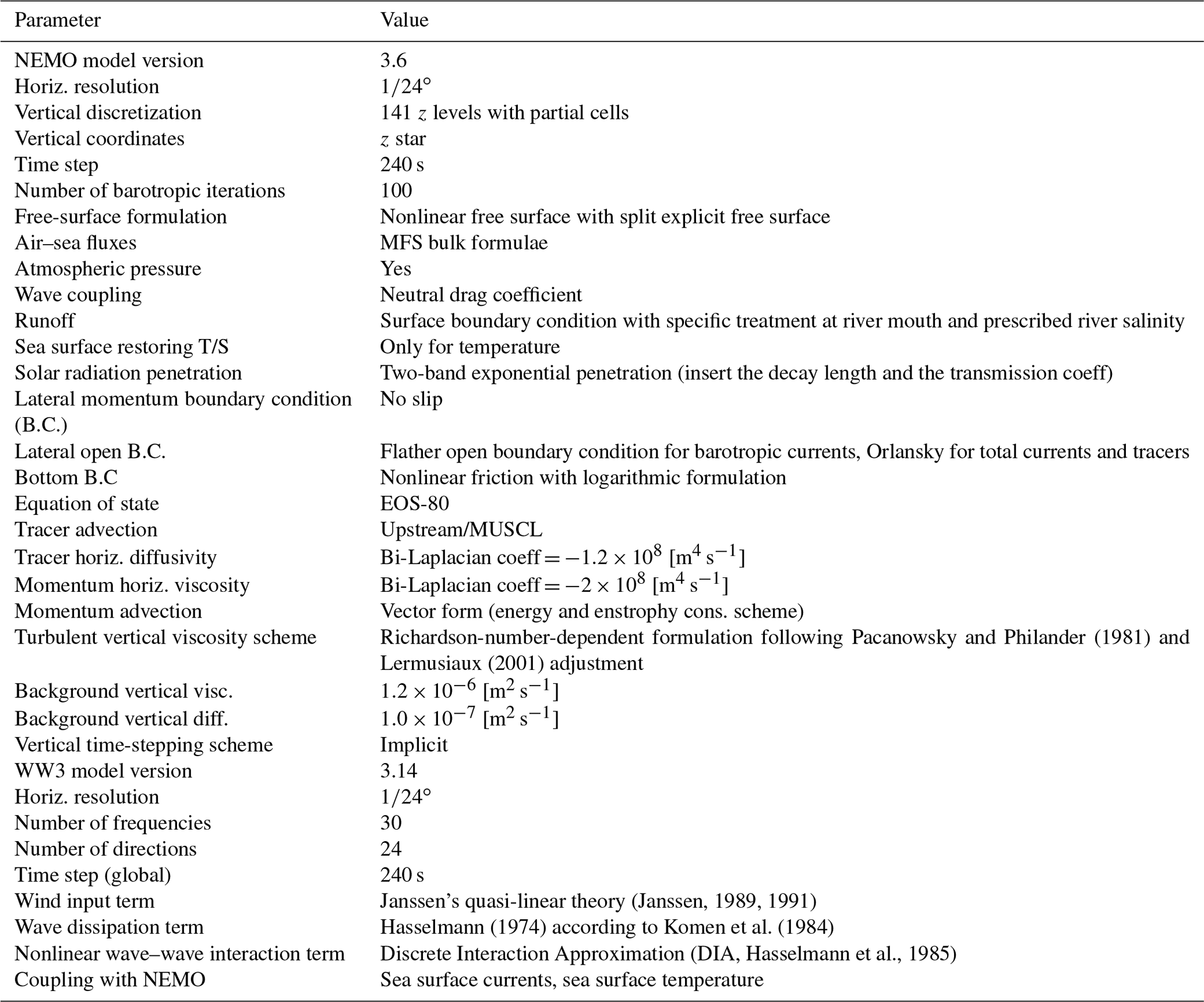
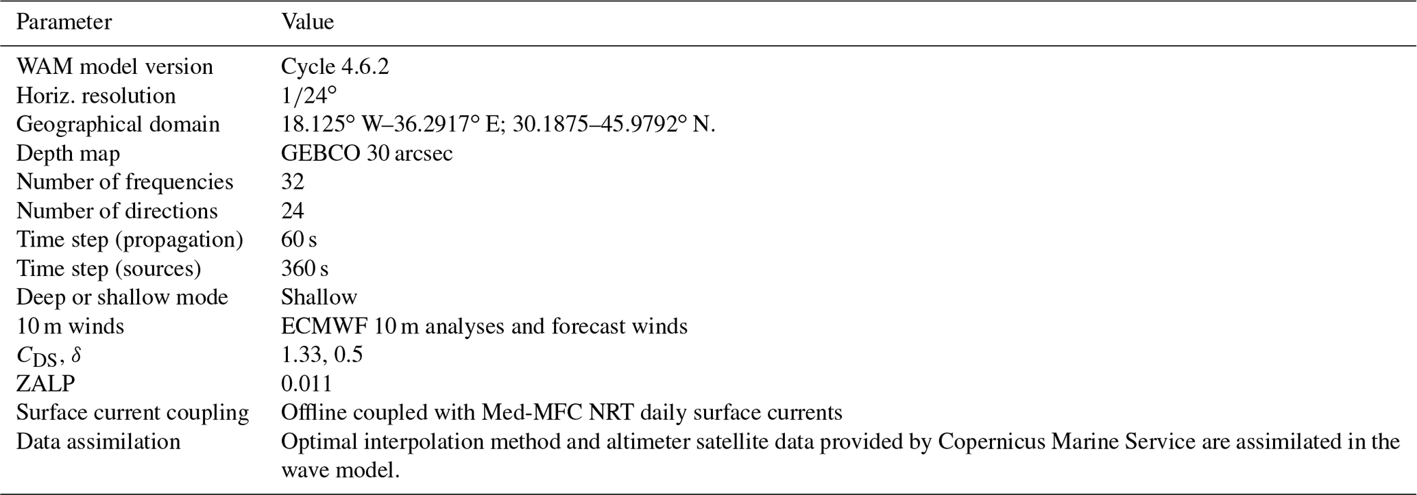
Table A3List of the OGSTM-BFM model setup for the BIO component.

Table A4River sources implemented as freshwater inputs in the physical and biogeochemical models, including river name, the annual mean runoff, and the imposed salinity at the river mouth.
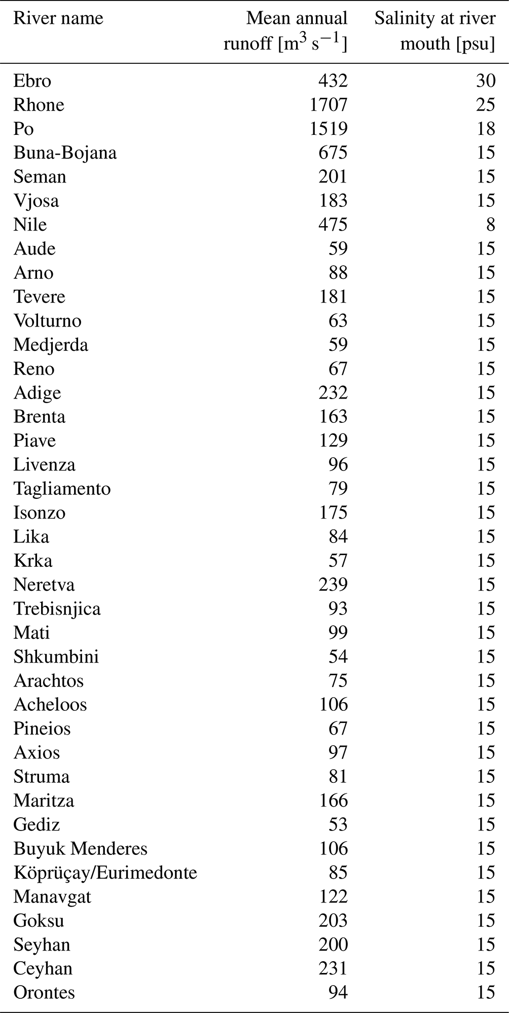
Data sets and codes used in this paper are available in the Supplement.
The supplement related to this article is available online at: https://doi.org/10.5194/os-19-1483-2023-supplement.
GCop and EC coordinated the preparation of the paper in collaboration with GCos and GK.
EC, GCos, GK, PL, AT, GB, JP, ACG, AA, RE, AC, DD, SM, AN, NP, and MR contributed to the system and model development; VL, AG, LF, CA, VDB, AM, ACG, AZ, CO, and EC contributed to the model validation and assessment; RL, MD, AM, AB, and GCoi contributed to the operational activities. All the authors contributed to the final version of the paper.
The contact author has declared that none of the authors has any competing interests.
Publisher’s note: Copernicus Publications remains neutral with regard to jurisdictional claims made in the text, published maps, institutional affiliations, or any other geographical representation in this paper. While Copernicus Publications makes every effort to include appropriate place names, the final responsibility lies with the authors.
This study has been conducted using EU Copernicus Marine Service Information. Within the Copernicus Marine Service of the Med-MFC, CMCC is in charge of the coordination of the service and is responsible for the physics (ocean circulation) production unit, OGS is responsible for the BIO (biogeochemical) production unit, and HCMR is responsible for the wave production unit. The authors thank CINECA (Italian supercomputer centre) for the technical support provided in the biogeochemical component production workflow. The authors thank Giorgia Verri (CMCC), George Zodiatis, and the Orion team for the collaboration in the development of the atmospheric forcing validation tool. The authors thank the anonymous reviewers for their valuable revisions.
This work has been funded through the EU Copernicus Marine Med-MFC Service (contract no. 74).
This paper was edited by Bernadette Sloyan and reviewed by three anonymous referees.
Adani, M., Dobricic, S., and Pinardi, N.: Quality Assessment of a 1985–2007 Mediterranean Sea Reanalysis, J. Atmos. Ocean. Tech., 28, 569–589, https://doi.org/10.1175/2010JTECHO798.1, 2011.
Álvarez, M., Sanleón-Bartolomé, H., Tanhua, T., Mintrop, L., Luchetta, A., Cantoni, C., Schroeder, K., and Civitarese, G.: The CO2 system in the Mediterranean Sea: a basin wide perspective, Ocean Sci., 10, 69–92, https://doi.org/10.5194/os-10-69-2014, 2014.
Alvarez Fanjul, E., Ciliberti, S., and Bahurel, P.: Implementing Operational Ocean Monitoring and Forecasting Systems, IOC-UNESCO, Paris, France, 376 pp., Annexes, GOOS-275, https://doi.org/10.48670/ETOOFS, 2022.
Ardhuin, F., Bertotti, L., Bidlot, J. R., Cavaleri, L., Filipetto, V., Lefevre, J. M., and Wittmann, P.: Comparison of wind and wave measurements and models in the Western Mediterranean Sea, Ocean Eng., 34, 526–541, https://doi.org/10.1016/j.oceaneng.2006.02.008, 2007.
Ayoub, N., Le Traon, P.-Y., and De Mey, P.: A description of the Mediterranean surface variable circulation from combined ERS-1 and Topex/Poseidon altimetric data, J. Marine Syst., 18, 3–40, 1998.
Bakker, D. C. E., Pfeil, B., Smith, K., Hankin, S., Olsen, A., Alin, S. R., Cosca, C., Harasawa, S., Kozyr, A., Nojiri, Y., O'Brien, K. M., Schuster, U., Telszewski, M., Tilbrook, B., Wada, C., Akl, J., Barbero, L., Bates, N. R., Boutin, J., Bozec, Y., Cai, W.-J., Castle, R. D., Chavez, F. P., Chen, L., Chierici, M., Currie, K., de Baar, H. J. W., Evans, W., Feely, R. A., Fransson, A., Gao, Z., Hales, B., Hardman-Mountford, N. J., Hoppema, M., Huang, W.-J., Hunt, C. W., Huss, B., Ichikawa, T., Johannessen, T., Jones, E. M., Jones, S. D., Jutterström, S., Kitidis, V., Körtzinger, A., Landschützer, P., Lauvset, S. K., Lefèvre, N., Manke, A. B., Mathis, J. T., Merlivat, L., Metzl, N., Murata, A., Newberger, T., Omar, A. M., Ono, T., Park, G.-H., Paterson, K., Pierrot, D., Ríos, A. F., Sabine, C. L., Saito, S., Salisbury, J., Sarma, V. V. S. S., Schlitzer, R., Sieger, R., Skjelvan, I., Steinhoff, T., Sullivan, K. F., Sun, H., Sutton, A. J., Suzuki, T., Sweeney, C., Takahashi, T., Tjiputra, J., Tsurushima, N., van Heuven, S. M. A. C., Vandemark, D., Vlahos, P., Wallace, D. W. R., Wanninkhof, R., and Watson, A. J.: An update to the Surface Ocean CO2 Atlas (SOCAT version 2), Earth Syst. Sci. Data, 6, 69–90, https://doi.org/10.5194/essd-6-69-2014, 2014.
Bakker, D. C. E., Pfeil, B. Landa, C. S., Metzl, N., O’Brien, K. M., Olsen, A., Smith, K., Cosca, C., Harasawa, S., Jones, S. D., Nakaoka, S., Nojiri, Y., Schuster, U., Steinhoff, T., Sweeney, C., Takahashi, T., Tilbrook, B., Wada, C., Wanninkhof, R., Alin, S. R., Balestrini, C. F., Barbero, L., Bates, N. R., Bianchi, A. A., Bonou, F., Boutin, J., Bozec, Y., Burger, E. F., Cai, W.-J., Castle, R. D., Chen, L., Chierici, M., Currie, K., Evans, W., Featherstone, C., Feely, R. A., Fransson, A., Goyet, C., Greenwood, N., Gregor, L., Hankin, S., Hardman-Mountford, N. J., Harlay, J., Hauck, J., Hoppema, M., Humphreys, M. P., Hunt, C. W., Huss, B., Ibánhez, J. S. P., Johannessen, T., Keeling, R., Kitidis, V., Körtzinger, A., Kozyr, A., Krasakopoulou, E., Kuwata, A., Landschützer, P., Lauvset, S. K., Lefèvre, N., Lo Monaco, C., Manke, A., Mathis, J. T., Merlivat, L., Millero, F. J., Monteiro, P. M. S., Munro, D. R., Murata, A., Newberger, T., Omar, A. M., Ono, T., Paterson, K., Pearce, D., Pierrot, D., Robbins, L. L., Saito, S., Salisbury, J., Schlitzer, R., Schneider, B., Schweitzer, R., Sieger, R., Skjelvan, I., Sullivan, K. F., Sutherland, S. C., Sutton, A. J., Tadokoro, K., Telszewski, M., Tuma, M., Van Heuven, S. M. A. C., Vandemark, D., Ward, B., Watson, A. J., and Xu, S.: A multi-decade record of high quality fCO2 data in version 3 of the Surface Ocean CO2 Atlas (SOCAT), Earth Syst. Sci. Data, 8, 383–413, https://doi.org/10.5194/essd-8-383-2016, 2016.
Barton, N., Metzger, E. J., Reynolds, C. A., Ruston, B., Rowley, C., Smedstad, O. M., Ridout, J. A., Wallcraft, A., Frolov, S., Hogan, P., Janiga, M. A., Shriver, J. F., McLay, J., Thoppil, P., Huang, A., Crawford, W., Whitcomb, T., Bishop, C. H., Zamudio, L., and Phelps, M.: The Navy's Earth System Prediction Capability: A new global coupled atmosphere-ocean-sea ice prediction system designed for daily to subseasonal forecasting, Earth Space Sci., 8, e2020EA001199, https://doi.org/10.1029/2020EA001199, 2021.
Bergamasco, A. and Malanotte-Rizzoli, P.: The circulation of the Mediterranean Sea: a historical review of experimental investigations, Adv. Oceanogr. Limnol., 1, 11–28, https://doi.org/10.1080/19475721.2010.491656, 2010.
Boyer, T. P., García, H. E., Locarnini, R. A., Zweng, M. M., Mishonov, A. V., Reagan, J. R., Weathers, K. A., Baranova, O. K., Paver, C. R., Seidov, D., and Smolyar, I. V.: World Ocean Atlas, NOAA National Centers for Environmental Information [data set], https://www.ncei.noaa.gov/archive/accession/NCEI-WOA18 (last access: 30 November 2022), 2018.
Brassington, G. B.: Forecast Errors, Goodness, and Verification in Ocean Forecasting, J. Mar. Res., 75, 403–433, https://doi.org/10.1357/002224017821836851, 2017.
Bruschi, A., Lisi, I., De Angelis, R., Querin, S., Cossarini, G., Di Biagio, V., et al.: Indexes for the assessment of bacterial pollution in bathing waters from point sources: The northern Adriatic Sea CADEAU service, J. Environ. Manage., 293, 112878, https://doi.org/10.1016/j.jenvman.2021.112878, 2021.
Buga, L., Sarbu, G., Fryberg, L., Magnus, W., Wesslander, K., Gatti, J., D., Leroy, D., Iona, S., Larsen, M., Østrem A.K., Schlitzer, R., Lipizer, M., Molina, E., and Giorgetti, A.: EMODnet Chemistry Eutrophication and Acidity aggregated datasets v2018, https://doi.org/10.6092/EC8207EF-ED81-4EE5-BF48-E26FF16BF02E, 2018.
Buongiorno Nardelli, B., Tronconi, C., Pisano, A., and Santoleri, R.: High and Ultra-High resolution processing of satellite Sea Surface Temperature data over Southern European Seas in the framework of MyOcean project, Remote Sens. Environ., 129, 1–16, https://doi.org/10.1016/j.rse.2012.10.012, 2013.
Byun, D. S. and Pinardi, N.: Comparison of Marine Insolation Estimating methods in the Adriatic Sea, Ocean Sci. J., 42, 211–222, 2007.
Candela, J.: Mediterranean water and global circulation, in: Ocean Circulation and Climate, edited by: Siedler, G., Church, J., and Gould, J., 419–429, Academic Press, San Diego, Ca, 2001.
Canu, D., Solidoro, C., Bandelj, V., Quattrocchi, G., Sorgente, R., Olita, A, Fazioli, L., and Cucco, A.: Assessment of oil slick hazard and risk at vulnerable coastal sites, Mar. Pollut. Bull., 94, https://doi.org/10.1016/j.marpolbul.2015.03.006, 2015.
Carrassi, A., Bocquet, M., Bertino, L., and Evensen, G.: Data assimilation in the geosciences: An overview of methods, issues, and perspectives, WIRes Clim. Change, 9, e535, https://doi.org/DOI:10.1002/wcc.535, 2018.
Cavaleri, L. and Sclavo, M.: The calibration of wind and wave model data in the Mediterranean Sea, Coast. Eng., 53, 613–627, 2006.
Cessi, P., Pinardi, N., and Lyubartsev, V.: Energetics of Semienclosed Basins with Two-Layer Flows at the Strait, J. Phys. Oceanogr., 44, 967–979, https://doi.org/10.1175/JPO-D-13-0129.1, 2014.
Cliberti, S. A., Jansen, E., Coppini, G., Peneva, E., Azevedo, D., Causio, S., Stefanizzi, L., Cretì, S., Lecci, R., Lima L., Ilicak M., Pinardi, N., and Palazov, A.: The Black Sea Physics Analysis and Forecasting System within the Framework of the Copernicus Marine Service, J. Mar. Sci. Eng., 10, 48, https://doi.org/10.3390/jmse10010048, 2022.
Clementi, E., Oddo, P., Drudi, M., Pinardi, N., Korres, G., and Grandi, A.: Coupling hydrodynamic and wave models: first step and sensitivity experiments in the Mediterranean Sea, Ocean Dynam., 67, 1293–1312, https://doi.org/10.1007/s10236-017-1087-7, 2017a.
Clementi, E., Pistoia, J., Delrosso, D., Mattia, G., Fratianni, C., Storto, A., Ciliberti, S., Lemieux, B., Fenu, E., Simoncelli, S., Drudi, M., Grandi, A., Padeletti, D., Di Pietro, P., and Pinardi, N.: A degree resolution Mediterranean analysis and forecast modelling system for the Copernicus Marine Environment Monitoring Service, Extended abstract to the 8th EuroGOOS Conference, Bergen, http://eurogoos.eu/download/publications/EuroGOOS-2017-Conference-Proceedings.pdf (last access: 30 January 2023), 2017b.
Clementi, E., Pistoia, J., Escudier, R., Delrosso, D., Drudi, M., Grandi, A., Lecci, R., Cretí, S., Ciliberti, S., Coppini, G., Masina, S., and Pinardi, N.: Mediterranean Sea Analysis and Forecast (CMEMS MED-Currents EAS5 system, 2017–2020), Copernicus Monitoring Environment Marine Service (CMEMS) [data set], https://doi.org/10.25423/CMCC/MEDSEA_ANALYSIS_FORECAST_PHY_006_013_EAS5, 2019.
Copernicus Marine In-Situ Team and Copernicus In Situ TAC: Real Time Quality Control for WAVES, CMEMS-INS-WAVES-RTQC, Copernicus [data set], https://doi.org/10.13155/46607, 2020.
Copin-Montegut, C.: Alkalinity and carbon budgets in the Mediterranean Sea, Global Biogeochem. Cy., 7, 915–925, 1993.
Cossarini, G., Lazzari, P., and Solidoro, C.: Spatiotemporal variability of alkalinity in the Mediterranean Sea, Biogeosciences, 12, 1647–1658, https://doi.org/10.5194/bg-12-1647-2015, 2015.
Cossarini, G., Querin, S., Solidoro, C., Sannino, G., Lazzari, P., Di Biagio, V., and Bolzon, G.: Development of BFMCOUPLER (v1.0), the coupling scheme that links the MITgcm and BFM models for ocean biogeochemistry simulations, Geosci. Model Dev., 10, 1423–1445, https://doi.org/10.5194/gmd-10-1423-2017, 2017.
Cossarini, G., Mariotti, L., Feudale, L., Teruzzi, A., D'Ortenzio, F., Tallandier, V., and Mignot A.: Towards operational 3D-Var assimilation of chlorophyll Biogeochemical-Argo float data into a biogeochemical model of the Mediterranean Sea, Ocean Model., 133, 112–128, https://doi.org/10.1016/j.ocemod.2018.11.005, 2019.
Cossarini, G., Bretagnon, M., Di Biagio, V., Fanton d'Andon, O., Garnesson, P., Mangin, A., and Solidoro, C.: Primary production, Copernicus Marine Service Ocean State Report, Issue 4, J. Oper. Oceanogr., 12, s88–s91, https://doi.org/10.1080/1755876X.2020.1785097, 2020.
Cossarini, G., Feudale, L., Teruzzi, A., Bolzon, G., Coidessa, G., Solidoro, C., Di Biagio, V., Amadio, C., Lazzari, P., Brosich, A., and Salon, S.: High-resolution reanalysis of the Mediterranean Sea biogeochemistry (1999–2019), Frontiers in Marine Science, 8, 1537, https://doi.org/10.3389/fmars.2021.741486, 2021.
Deliverable of Perseus: Deliverable D4.6, SES land-based runoff and nutrient load data (1980–2000), edited by: Bouwman, L. and van Apeldoorn, D., 2012 PERSEUS H2020 grant agreement n. 287600, European Commission, http://www.perseus-net.eu/assets/media/PDF/deliverables/3321.6_Final.pdf (last access: 30 July 2023), 2012.
Delrosso, D.: Numerical modelling and analysis of riverine influences in the Mediterranean Sea, PhD Thesis, Alma Mater Studiorum Università di Bologna, https://doi.org/10.6092/unibo/amsdottorato/9392, 2020.
Desroziers, G., Berre, L., Chapnik, B., and Poli, P.: Diagnosis of observation, background and analysis-error statistics in observation space, Q. J. Roy. Meteor. Soc., 131, 3385–3396, https://doi.org/10.1256/qj.05.108, 2005.
Dickson, A. G.: Thermodynamics of the dissociation of boric acid in synthetic seawater from 273.15 to 318.15 K, Deep-Sea Res., 37, 755–766, 1990.
Dickson, A. G., Sabine, C. L., and Christian, J. R.: Guide to best practices for ocean CO2 measurements, North Pacific Marine Science Organization, Sidney, British Columbia, 191, https://doi.org/10.25607/OBP-1342, 2007.
Dobricic, S. and Pinardi, N.: An oceanographic three-dimensional variational data assimilation scheme, Ocean Model., 22, 89–105, https://doi.org/10.1016/j.ocemod.2008.01.004, 2008.
Dobricic, S., Pinardi, N., Adani, M., Tonani, M., Fratianni, C., Bonazzi, A., and Fernandez, V.: Daily oceanographic analyses by Mediterranean Forecasting System at the basin scale, Ocean Sci., 3, 149–157, https://doi.org/10.5194/os-3-149-2007, 2007.
Dobricic, S., Pinardi, N., Testor, P., and Send, U.: Impact of data assimilation of glider observations in the Ionian Sea (Eastern Mediterranean), Dynam. Atmos. Oceans, 50, 78–92, https://doi.org/10.1016/j.dynatmoce.2010.01.001, 2010.
Dobricic, S., Dufau, C., Oddo, P., Pinardi, N., Pujol, I., and Rio, M.-H.: Assimilation of SLA along track observations in the Mediterranean with an oceanographic model forced by atmospheric pressure, Ocean Sci., 8, 787–795, https://doi.org/10.5194/os-8-787-2012, 2012.
ECMWF: IFS Documentation CY43R1, Part VII: ECMWF Wave Model, Book chapter, ECMWF, https://doi.org/10.21957/18mel2ooj, 2016.
Escudier, R., Clementi, E., Omar, M., Cipollone, A., Pistoia, J., Aydogdu, A., Drudi, M., Grandi, A., Lyubartsev, V., Lecci, R., Cretí, S., Masina, S., Coppini, G., and Pinardi, N.: Mediterranean Sea Physical Reanalysis (CMEMS MED-Currents) (Version 1), Copernicus Monitoring Environment Marine Service (CMEMS) [data set], https://doi.org/10.25423/CMCC/MEDSEA_MULTIYEAR_PHY_006_004_E3R1, 2020.
Escudier, R., Clementi, E., Cipollone, A., Pistoia, J., Drudi, 50 M., Grandi, A., Lyubartsev, V., Lecci, R., Aydogdu, A., Delrosso, D., Mohamed O., Masina, S. Coppini, G., and Pinardi, N.: A High Resolution Reanalysis for the Mediterranean Sea, Front. Earth Sci., 9, 702285, https://doi.org/10.3389/feart.2021.702285, 2021.
Federico, I., Pinardi, N., Coppini, G., Oddo, P., Lecci, R., and Mossa, M.: Coastal ocean forecasting with an unstructured grid model in the southern Adriatic and northern Ionian seas, Nat. Hazards Earth Syst. Sci., 17, 45–59, https://doi.org/10.5194/nhess-17-45-2017, 2017.
Feudale, L., Bolzon, G., Lazzari, P., Salon, S., Teruzzi, A., Di Biagio, V., Coidessa, G., and Cossarini, G.: Mediterranean Sea Biogeochemical Analysis and Forecast (CMEMS MED-Biogeochemistry, MedBFM3 system) (Version 1), Copernicus Monitoring Environment Marine Service (CMEMS) [data set], https://doi.org/10.25423/CMCC/MEDSEA_ANALYSISFORECAST_BGC_006_014_MEDBFM3, 2021.
Flather, R. A.: A tidal model of the north–west European continental shelf, Mem. Soc. R. Sci. Liege, 10, 141–164, 1976.
Foujols, M.-A., Lévy, M., Aumont, O., and Madec, G.: OPA 8.1 Tracer Model Reference Manual Institut Pierre Simon Laplace, p. 39, 2000.
García-Lafuente, J. and Sánchez-Romn, A.: Estimation of the Atlantic inflow through the strait of Gibraltar from climatological and in situ data, J. Geophys. Res.-Ocean., 115, https://doi.org/10.1029/2010JC006302, 2010.
Giesen, R., Clementi, E., Bajo, M., Federico, I., Stoffelen, A., and Santoleri, R.: Copernicus Marine Service Ocean State Report, Issue 5, J. Oper. Oceanogr., 14, s140–s148, https://doi.org/10.1080/1755876X.2021.1946240, 2021.
Guenther, H., Hasselmann, S., and Janssen, P. A. E. M.: The WAM model cycle 4 (DKRZ-TR–4(reved)), Germany, 1992.
Hasselmann, K.: On the spectral dissipation of ocean waves due to whitecapping, Bound.-Lay. Meteorol., 126, 107–127, 1974.
Hasselmann, K., Barnett, T. P., Bouws, E., Carlson, H., Cartwright, D. E., Enke, K., Ewing, J. A., Gienapp, H., Hasselmann, D. E., Kruseman, P., Meerburg, A., Müller, P., Olbers, D. J., Richter, K., Sell, W., and Walden, H.: Measurements of wind–wave growth and swell decay during the Joint North Sea Wave Project (JONSWAP), Dtsch. Hydrogr. Z., 8, 1–95, 1973.
Hasselmann, K., Allender, J. H., and Barnett, T. P.: Computations and parameterizations of the nonlinear energy transfer in a gravity wave spectrum. Part II: Parameterizations of the nonlinear energy transfer for application in wave models, J. Phys. Oceanogr.,15, 1378–1391, 1985.
Hernandez, F., Bertino, L., Brassington, G., Chassignet, E., Cummings, J., Davidson, F., Drévillon, M., Garric, G., Kamachi, M. Lellouche, J.-M., Mahdon, R., Martin, M. J., Ratsimandresy, A., and Regnier, C.: Validation and intercomparison studies within GODAE, Oceanography, 22, 128–143, https://doi.org/10.5670/oceanog.2009.71, 2009.
Hernandez, F., Smith, G., Baetens, K., Cossarini, G., Garcia-Hermosa, I., Drevillon, M., Maksymczuk, J., Melet, A., Regnier, C., and von Schuckman, K.: Measuring Performances, Skill and Accuracy in Operational Oceanography: New Challenges and Approaches, in: New Frontiers in Operational Oceanography, edited by: Chassignet, E., Pascual, A., Tintoré, J., and Verron, J., GODAE OceanView, 759–796, https://doi.org/10.17125/gov2018.ch29, 2018.
Janssen, P. A. E. M.: Wave induced stress and the drag of air flow over sea wave, J. Phys. Oceanogr., 19, 745–754, 1989.
Janssen, P. A. E. M.: Quasi-Linear theory of wind wave generation applied to wave forecasting, J. Phys. Oceanogr., 21, 1631–1642, 1991.
Johnson, K., Pasqueron De Fommervault, O., Serr, R., D'Ortenzio, F., Schmechtig, C., Claustre, H., and Poteau, A.: Processing Bio-Argo nitrate concentration at the DAC Level, Version 1.1, IFREMER for Argo Data Management, 22 pp., https://doi.org/10.13155/46121, 2018.
Katsafados, P., Papadopoulos, A., Korres, G., and Varlas, G.: A fully coupled atmosphere–ocean wave modeling system for the Mediterranean Sea: interactions and sensitivity to the resolved scales and mechanisms, Geosci. Model Dev., 9, 161–173, https://doi.org/10.5194/gmd-9-161-2016, 2016.
Kempe, S., Pettine, M., and Cauwet, G.: Biogeochemistry of european rivers, in: Biogeochemistry of Major World Rivers, edited by: Degens, E. T., Kempe, S., and Richey, J. E., SCOPE, John Wiley, 169–211, 1991.
Komen, G. J., Hasselmann, S., and Hasselmann, K.: On the existence of a fully developed windsea spectrum, J. Phys. Oceanogr., 14, 1271–1285, 1984.
Komen G. J., Cavaleri, L., Donelan, M., Hasselmann, K., Hasselmann, S., and Janssen, P. A. E. M.: Dynamics and Modelling of Ocean Waves, 554 pp., ISBN 0521577810, Cambridge, UK, Cambridge University Press, 1996.
Korres, G., Papadopoulos, A., Katsafados, P., Ballas, D., Perivoliotis, L., and Nittis, K.: A 2-year intercomparison of the WAM-Cycle4 and the WAVEWATCH-III wave models implemented within the Mediterranean Sea, Mediterr. Mar. Sci., 12, 129-152, https://doi.org/10.12681/mms.57, 2011.
Krasakopoulou, E., Souvermezoglou, E., Giannoudi, L., and Goyet, C.: Carbonate system parameters ad anthropogenic CO2 in the North Aegean Sea during October 2013, Cont. Shelf Res., 149, 69–81, 2017.
Lazzari, P., Teruzzi, A., Salon, S., Campagna, S., Calonaci, C., Colella, S., Tonani, M., and Crise, A.: Pre-operational short-term forecasts for Mediterranean Sea biogeochemistry, Ocean Sci., 6, 25–39, https://doi.org/10.5194/os-6-25-2010, 2010.
Lazzari, P., Solidoro, C., Ibello, V., Salon, S., Teruzzi, A., Béranger, K., Colella, S., and Crise, A.: Seasonal and inter-annual variability of plankton chlorophyll and primary production in the Mediterranean Sea: a modelling approach, Biogeosciences, 9, 217–233, https://doi.org/10.5194/bg-9-217-2012, 2012.
Lazzari, P., Solidoro, C., Salon, S., and Bolzon, G.: Spatial variability of phosphate and nitrate in the Mediterranean Sea: a modelling approach, Deep-Sea Res. Pt. I, 108, 39–52, https://doi.org/10.1016/j.dsr.2015.12.006, 2016.
Lazzari, P., Álvarez, E., Terzić, E., Cossarini, G., Chernov, I., D'Ortenzio, F., and Organelli, E.: CDOM Spatiotemporal Variability in the Mediterranean Sea: A Modelling Study, J. Mar. Sci. Eng., 9, 176, https://doi.org/10.3390/jmse9020176, 2021.
Lellouche, J.-M., Greiner, E., Le Galloudec, O., Garric, G., Regnier, C., Drevillon, M., Benkiran, M., Testut, C.-E., Bourdalle-Badie, R., Gasparin, F., Hernandez, O., Levier, B., Drillet, Y., Remy, E., and Le Traon, P.-Y.: Recent updates to the Copernicus Marine Service global ocean monitoring and forecasting real-time ∘ high-resolution system, Ocean Sci., 14, 1093–1126, https://doi.org/10.5194/os-14-1093-2018, 2018.
Lermusiaux, O. F. J.: Evolving the subspace of the three-dimensional multiscale ocean variability: Massachusetts Bay, J. Marine Syst., 29, 385–422, https://doi.org/10.1016/S0924-7963(01)00025-2 2001.
Le Traon, P., Ali, A., Alvarez Fanjul, E., Behrens, A., Stanev, E., and Staneva, J.: The Copernicus Marine Environmental Monitoring Service: Main Scientific Achievements and Future Prospects: Special Issue Mercator Océan Journal, Vol. 56, https://doi.org/10.25575/56, 2017.
Le Traon, P. Y., Reppucci, A., Alvarez Fanjul, E., Aouf, L., Behrens, A., Belmonte, M., Bentamy, A., Bertino, L., Brando, V. E., Kreiner, M. B., Benkiran, M., Carval, T., Ciliberti, S. A., Claustre, H., Clementi, E., Coppini, G., Cossarini, G., De Alfonso Alonso-Muñoyerro, M., Delamarche, A., Dibarboure, G., Dinessen, F., Drevillon, M., Drillet, Y., Faugere, Y., Fernández, V., Fleming, A., Garcia-Hermosa, M. I., Sotillo, M. G., Garric, G., Gasparin, F., Giordan, C., Gehlen, M., Gregoire, M. L., Guinehut, S., Hamon, M., Harris, C., Hernandez, F., Hinkler, J. B., Hoyer, J., Karvonen, J., Kay, S., King, R., Lavergne, T., Lemieux-Dudon, B., Lima, L., Mao, C., Martin, M. J., Masina, S., Melet, A., Buongiorno Nardelli, B., Nolan, G., Pascual, A., Pistoia, J., Palazov, A., Piolle, J. F., Pujol, M. I., Pequignet, A. C., Peneva, E., Pérez Gómez, B., Petit de la Villeon, L., Pinardi, N., Pisano, A., Pouliquen, S., Reid, R., Remy, E., Santoleri, R., Siddorn, J., She, J., Staneva, J., Stoffelen, A., Tonani, M., Vandenbulcke, L., von Schuckmann, K., Volpe, G., Wettre, C., and Zacharioudaki, A.: From Observation to Information and Users: The Copernicus Marine Service Perspective, Front. Mar. Sci., 6, 234, https://doi.org/10.3389/fmars.2019.00234, 2019.
Levy, M., Estubier, A., and Madec, G.: Choice of an advection scheme for biogeochemical models, Geophys. Res. Lett., 28, https://doi.org/10.1029/2001GL012947, 2001.
Lionello, P., Gunther, H., and Janssen, P. A. E. M.: Assimilation of altimeter data in a global third generation wave model, J. Geophys. Res., 97C, 14453–14474, 1992.
Lueker, T. J., Dickson, A. G., and Keeling, C. D.: Ocean pCO2 calculated from dissolved inorganic carbon, alkalinity, and equations for K1 and K2: validation based on laboratory measurements of CO2 in gas and seawater at equilibrium, Mar. Chem., 70, 105–119, 2000.
Madec, G. and the NEMO system Team: NEMO Ocean Engine, Scientific Notes of Climate Modelling Center (27), Institut Pierre-Simon Laplace (IPSL), Zenodo , https://doi.org/10.5281/zenodo.1472492, 2019.
Madec, G., Delecluse, P., Imbard, M., and Levy, C.: OPA8.1 Ocean general Circulation Model reference m anual, Note du Pole de modelisazion, Institut Pierre-Simon Laplace (IPSL), France, 11 pp., 1998.
Maderich, V., Ilyin, Y., and Lemeshko, E.: Seasonal and interannual variability of the water exchange in the Turkish Straits System estimated by modelling, Mediterr. Mar. Sci., 16, 444–459, https://doi.org/10.12681/mms.1103, 2015.
Mannarini, G., Turrisi, G., D'Anca, A., Scalas, M., Pinardi, N., Coppini, G., Palermo, F., Carluccio, I., Scuro, M., Cretì, S., Lecci, R., Nassisi, P., and Tedesco, L.: VISIR: technological infrastructure of an operational service for safe and efficient navigation in the Mediterranean Sea, Nat. Hazard. Earth Syst. Sci., 16, 1791–1806, https://doi.org/10.5194/nhess-16-1791-2016, 2016a.
Mannarini, G., Pinardi, N., Coppini, G., Oddo, P., and Iafrati, A.: VISIR-I: small vessels – least-time nautical routes using wave forecasts, Geosci. Model Dev., 9, 1597–1625, https://doi.org/10.5194/gmd-9-1597-2016, 2016b.
Mannarini, G. and Carelli, L.: VISIR-1.b: ocean surface gravity waves and currents for energy-efficient navigation, Geosci. Model Dev., 12, 3449–3480, https://doi.org/10.5194/gmd-12-3449-2019, 2019.
Marchesiello, P., McWilliams, J. C., and Shchepetkin, A.: Open boundary conditions for long-term integration of regional oceanic models, Ocean Model., 3, 1–20, 2001.
McEwan, R., Kay, S., and Ford, D.: Quality Information Document of NWSHELF_ANALYSISFORECAST_BGC_004_002, Marine Copernicus Service, https://catalogue.marine.copernicus.eu/documents/QUID/CMEMS-NWS-QUID-004-002.pdf (last access: 15 July 2022), 2021.
McGovern, J. V., Dabrowski, T., Pereiro, D., Gutknecht, E., Lorente, P., Reffray, G., Aznar, R., and Sotillo, M. G.: Quality Information Document of IBI_ANALYSISFORECAST_BGC_005_004, Marine Copernicus Service, https://catalogue.marine.copernicus.eu/documents/QUID/CMEMS-IBI-QUID-005-004.pdf (last access: 15 July 2022), 2020.
Melsom, A. and Yumruktepe, Ç.: Quality Information Document of ARTIC_ANALYSIS_FORECAST_BIO_002_004, Marine Copernicus Service, https://catalogue.marine.copernicus.eu/documents/QUID/CMEMS-ARC-QUID-002-004.pdf (last access: 15 July 2022), 2021.
Meybeck, M. and Ragu, A.: River Discarges to the Oceans: An Assessment of suspended solids, major ions and nutrients UNEP STUDY, 1995.
Millero, F. J.: Thermodynamics of the carbon dioxide system in the oceans, Geochim. Cosmochim. Ac., 59, 661–677, 1995.
Millero, F., Schrager, S., and Hansen, L.: Thermometric titration analysis of seawater for chlorinity, sulfate, and alkalinity, Limnol. Oceanogr., 19, 711–715, https://doi.org/10.4319/lo.1974.19.4.0711, 1974.
Milliff, R. F., Bonazzi, A., Wikle, C. K., Pinardi, N., and Berliner, L. M.: Ocean ensemble forecasting, Part I: EnsembleMediterranean winds from a Bayesian hierarchical model, Q. J. R. Meteorol. Soc, 137, 858–878, https://doi.org/10.1002/qj.767, 2011.
Munhoven, G.: Mathematics of the total alkalinity-pH equation-Pathway to robust and universal solution algorithms: The SolveSAPHE package v1.0.1, Geosci. Model Dev., 6, 1367–1388, https://doi.org/10.5194/gmd-6-1367-2013, 2013.
Nagy, H., Lyons, K., Nolan, G., Cure, M., and Dabrowski, T.: A Regional Operational Model for the North East Atlantic: Model Configuration and Validation, J. Mar. Sci. Eng., 8, 673, https://doi.org/10.3390/jmse8090673, 2020.
Napolitano, E., Iacono, R., Palma, M., Sannino, G., Carillo, A., Lombardi, E., Pisacane, G., and Struglia, M. V.: MITO: A new operational model for the forecasting of the Mediterranean sea circulation, Front. Energy Res., 10, 941606, https://doi.org/10.3389/fenrg.2022.941606, 2022.
Nilsson, J., Dobricic, S., Taillandier, V., Poulain, P.-M., and Pinardi, N.: On the Assimilation of Argo Float Trajectories into the Mediterranean Forecasting System, 12, 7002, https://doi.org/10.1007/s10236-011-0437-0, 2010.
NOAA National Centers for Environmental Information: ETOPO 2022 15 Arc-Second Global Relief Model, NOAA National Centers for Environmental Information, https://doi.org/10.25921/fd45-gt74, 2022.
Oddo, P., Adani, M., Pinardi, N., Fratianni, C., Tonani, M., and Pettenuzzo, D.: A nested Atlantic-Mediterranean Sea general circulation model for operational forecasting, Ocean Sci., 5, 461–473, https://doi.org/10.5194/os-5-461-2009, 2009.
Oddo, P., Bonaduce, A., Pinardi, N., and Guarnieri, A.: Sensitivity of the Mediterranean sea level to atmospheric pressure and free surface elevation numerical formulation in NEMO, Geosci. Model Dev., 7, 3001–3015, https://doi.org/10.5194/gmd-7-3001-2014, 2014.
Oreskes, N., Shrader-Frechette, K., and Belitz, K.: Verification, validation, and confirmation of numerical models in the Earth sciences, Science, 263, 641–646, https://doi.org/10.1126/science.263.5147.641, 1994.
Orlanski, I.: A simple boundary condition for unbounded hyperbolic flows, J. Comput. Phys., 21, 251–269, 1976.
Pacanowski, R. C. and Philander, S. G. H.: Parameterization of vertical mixing in numerical models of tropical oceans, J. Phys. Oceanogr., 11, 1443–1451, https://doi.org/10.1175/1520-0485(1981)011<1443:POVMIN>2.0.CO;2, 1981.
Perez, F. F. and Fraga, F.: Association constant of fluoride and hydrogen ions in seawater, Mar. Chem., 21, 161–168, 1987.
Pettenuzzo, D., Large, W. G., and Pinardi, N.: On the corrections of ERA-40 surface flux products consistent with the Mediterranean heat and water budgets and the connection between basin surface total heat flux and NAO, J. Geophys. Res., 115, C06022, https://doi.org/10.1029/2009JC005631, 2010.
Pinardi, N., Allen, I., Demirov, E., De Mey, P., Korres, G., Lascaratos, A., Le Traon, P.-Y., Maillard, C., Manzella, G., and Tziavos, C.: The Mediterranean ocean Forecasting System: first phase of implementation (1998–2001), Ann. Geophys., 21, 3–20, https://doi.org/10.5194/angeo-21-3-2003, 2003.
Pinardi, N. and Coppini, G.: Preface “Operational oceanography in the Mediterranean Sea: the second stage of development”, Ocean Sci., 6, 263–267, https://doi.org/10.5194/os-6-263-2010, 2010.
Pinardi, N., Arneri, E., Crise, A., Ravaioli, M., and Zavatarelli, M.: The physical, sedimentary and ecological structure and variability of shelf areas in the Mediterranean Sea, in: The Sea, edited by: Robinson, A. R. and Brink, K., Vol. 14, Harvard University Press, Cambridge, USA, 1243–1330, 2006.
Pinardi, N., Bonazzi, A., Dobricic, S., Milliff, R. F., Wikle, C. K., and Berliner, L. M.: Ocean ensemble forecasting, Part II: Mediterranean Forecast System response, Q. J. R. Meteorol. Soc., 137, 879–893, https://doi.org/10.1002/qj.816, 2011.
Pinardi, N., Zavatarelli, M., Adani, M., Coppini, G., Fratianni, C., Oddo, P., Simoncelli, S., Tonani, M., Lyubartsev, V., Dobricic, S., and Bonaduce, A.: Mediterranean Sea large-scale low-frequency ocean variability and water mass formation rates from 1987 to 2007: A retrospective analysis, Prog. Oceanogr., 132, 318–332, https://doi.org/10.1016/j.pocean.2013.11.003, 2015.
Pinardi, N., Lermusiaux, P. F. J., Brink, K. H., and Preller, R. H.: The Sea: The science of ocean predictions, J. Marine Res., 75, 101–102, https://doi.org/10.1357/002224017821836833, 2017.
Pinardi, N., Cessi, P., Borile, F., and Wolfe, C. L.: The Mediterranean Sea Overturning Circulation, J. Phys. Oceanogr., 49, 1699–1721, https://doi.org/10.1175/JPO-D-18-0254.1, 2019.
Pineau-Guillou, L., Ardhuin, F., Bouin, M.-N., Redelsperger, J.-L., Chapron, B., Bidlot, J.-R., and Quilfen Y.: Strong winds in a coupled wave-atmosphere model during a North Atlantic storm event: evaluation against observations, Q. J. Roy. Meteor. Soc., 144, 317–332, https://doi.org/10.1002/qj.3205, 2018.
Pistoia, J., Clementi, E., Delrosso, D., Mattia, G., Fratianni, C., Drudi, M., Grandi, A., Paleletti, D., Di Pietro, P., Storto, A., and Pinardi, N.: Last improvements in the data assimilation scheme for the Mediterranean Analysis and Forecast system of the Copernicus Marine Service, Extended abstract to the 8th EuroGOOS Conference 2017, Bergen, http://eurogoos.eu/download/publications/EuroGOOS-2017-Conference-Proceedings.pdf (last access: 1 June 2023), 2017.
Ravdas, M., Zacharioudaki, A., and Korres, G.: Implementation and validation of a new operational wave forecasting system of the Mediterranean Monitoring and Forecasting Centre in the framework of the Copernicus Marine Environment Monitoring Service, Nat. Hazards Earth Syst. Sci., 18, 2675–2695, https://doi.org/10.5194/nhess-18-2675-2018, 2018.
Reed, R. K.: On estimating insolation over the ocean, J. Phys. Oceanogr., 7, 482–485, 1977.
Ribera d'Alcalà, M., Civitarese, G., Conversano, F., and Lavezza, R.: Nutrient ratios and fluxes hint at overlooked processes in the Mediterranean Sea, J. Geophys. Res., 108, 8106, https://doi.org/10.1029/2002JC001650, 2003.
Robinson, A. R., Leslie, W. G., Theocharis, A., and Lascartos, A.: Mediterranean Sea Circulation, Encyclopedia of Ocean Sciences, 2001, 1689–1705, https://doi.org/10.1006/rwos.2001.0376, 2001.
Salon, S., Cossarini, G., Bolzon, G., Feudale, L., Lazzari, P., Teruzzi, A., Solidoro, C., and Crise, A.: Novel metrics based on Biogeochemical Argo data to improve the model uncertainty evaluation of the CMEMS Mediterranean marine ecosystem forecasts, Ocean Sci., 15, 997–1022, https://doi.org/10.5194/os-15-997-2019, 2019.
Schneider, A., Wallace, D. W. R., and Kortzinger, A.: Alkalinity of the Mediterranean Sea, Geophys. Res. Lett., 34, L15608, https://doi.org/10.1029/2006GL028842, 2007.
Schmechtig, C., Poteau, A., Claustre, H., D'Ortenzio, F., Dall'Olmo, G., and Boss, E.: Processing Bio-Argo particle backscattering at the DAC level, Argo, https://doi.org/10.13155/39468, 2018.
Simoncelli, S., Fratianni, C., Pinardi, N., Grandi, A., Drudi, M., Oddo, P., and Dobricic, S.: Mediterranean Sea Physical Reanalysis (CMEMS MED-Physics) (Version 1), Copernicus Monitoring Environment Marine Service (CMEMS) [data set], https://doi.org/10.25423/MEDSEA_REANALYSIS_PHYS_006_004, 2019.
Siokou-Frangou, I., Christaki, U., Mazzocchi, M. G., Montresor, M., Ribera d'Alcalá, M., Vaqué, D., and Zingone, A.: Plankton in the open Mediterranean Sea: a review, Biogeosciences, 7, 1543–1586, https://doi.org/10.5194/bg-7-1543-2010, 2010.
Snyder, R. L., Dobson, F. W., Elliot, J. A., and Long, R. B.: Array measurements of atmospheric pressure fluctuations above surface gravity waves, J. Fluid Mech., 102, 1–59, 1981.
Sotillo, M. G., Garcia-Hermosa, I., Drévillon, M., Régnier, C., Szczypta, C., Hernandez, F., Melet, A., and Le Traon, P. Y.: Communicating CMEMS Product Quality: evolution & achievements along Copernicus-1 (2015–2021), Mercator Ocean J., no. 57, https://marine.copernicus.eu/it/node/19306 (last access: 1 July 2023), 2021.
Soto-Navarro, J., Criado-Aldeanueva F.,, García-Lafuente, J., and Sánchez-Romn, A.: Estimation of the Atlantic inflow through the strait of Gibraltar from climatological and in situ data, J. Geophys. Res.-Ocean., 115, https://doi.org/10.1029/2010JC006302, 2010.
Souvermezoglou, E., Krasakopoulou, E., and Pavlidou, A.: Temporal and spatial variability of nutrients and oxygen in the North Aegean Sea during the last thirty years, Mediterr. Mar. Sci., 15, 805–822, 2014.
Spruch L., Verjovkina, S., Jandt, S., Schwichtenberg, F., Huess, V., Lorkowski, I., and Lagemaa, P.: Quality Information Document of BALTICSEA_ANALYSIS_FORECAST_BIO_003_007, Marine Copernicus Service, https://catalogue.marine.copernicus.eu/documents/QUID/CMEMS-BAL-QUID-003-007.pdf (last access: 15 July 2022), 2020.
Storto, A., Dobricic, S., Masina, S., and Di Pietro,P.: Assimilating Along-track Altimetric Observations through Local Hydrostatic Adjustment in a Global Ocean Variational Assimilation System, Mon. Weather Rev., 3, 139, 2011.
Storto, A., Masina, S., and Dobricic, S.: Estimation and impact of nonuniform horizontal correlation length scales for global ocean physical analyses, J. Atmos. Ocean Technol. 31, 2330–2349, https://doi.org/10.1175/JTECH-D-14-00042.1, 2014.
Storto, A., Masina, S., and Navarra, A.: Evaluation of the CMCC eddy-permitting global ocean physical reanalysis system (C-GLORS, 1982–2012) and its assimilation components, Q. J. Roy. Meteor. Soc., 142, 738–758, https://doi.org/10.1002/qj.2673, 2015.
Taburet, G., Sanchez-Roman, A., Ballarotta, M., Pujol, M.-I., Legeais, J.-F., Fournier, F., Faugere, Y., and Dibarboure, G.: DUACS DT2018: 25 years of reprocessed sea level altimetry products, Ocean Sci., 15, 1207–1224, https://doi.org/10.5194/os-15-1207-2019, 2019.
Terzic, E., Salon, S., Solidoro, C., Cossarini, G., Teruzzi, A., Miro, A., and Lazzari, P.: Impact of interannually variable diffuse attenuation coefficients for downwelling irradiance on biogeochemical modelling, Ocean Model., OCEMOD-D-20-00012R2, https://doi.org/10.1016/j.ocemod.2021.101793, 2021.
Teruzzi, A., Dobricic, S., Solidoro, C., and Cossarini, G.: A 3D variational assimilation scheme in coupled transport biogeochemical models: Forecast of Mediterranean biogeochemical properties, J. Geophys. Res.-Oceans, 119, 200–217, https://doi.org/10.1002/2013JC009277, 2014.
Teruzzi, A., Bolzon, G., Salon, S., Lazzari, P., Solidoro, C., and Cossarini, G.: Assimilation of coastal and open sea biogeochemical data to improve phytoplankton modelling in the Mediterranean Sea, Ocean Model., 132, 46–60, https://doi.org/10.1016/j.ocemod.2018.09.007, 2018.
Teruzzi, A., Di Cerbo, P., Cossarini, G., Pascolo, E., and Salon, S.: Parallel implementation of a data assimilation scheme for operational oceanography: the case of the OGSTM-BFM model system, Comput. Geosci., 124, 103–114, https://doi.org/10.1016/j.cageo.2019.01.003, 2019.
Teruzzi, A., Bolzon, G., Feudale, L., and Cossarini, G.: Deep chlorophyll maximum and nutricline in the Mediterranean Sea: emerging properties from a multi-platform assimilated biogeochemical model experiment, Biogeosciences, 18, 6147–6166, https://doi.org/10.5194/bg-18-6147-2021, 2021.
Thoppil, P., G., Frolov, S., Rowley, C. D., Reynolds, C. A., Jacobs, G. A., Metzger, E. J., Hogan, P. J., Barton, N., Wallcraft, A. J., Smedstad, O. M., and Shriver, J. F.: Ensemble forecasting greatly expands the prediction horizon for ocean mesoscale variability, Commun. Earth Environ., 2, 89, https://doi.org/10.1038/s43247-021-00151-5, 2021.
Toledano, C., Ghantous, M., Lorente, P., Dalphinet, A., Aouf, L., and Sotillo, M. G.: Impacts of an Altimetric Wave Data Assimilation Scheme and Currents-Wave Coupling in an Operational Wave System: The New Copernicus Marine IBI Wave Forecast Service, J. Mar. Sci. Eng., 10, 457, https://doi.org/10.3390/jmse10040457, 2022.
Tonani, M., Pinardi, N., Dobricic, S., Pujol, I., and Fratianni, C.: A high-resolution free-surface model of the Mediterranean Sea, Ocean Sci., 4, 1–14, https://doi.org/10.5194/os-4-1-2008, 2008.
Tonani, M., Balmaseda, M., Bertino, L., Blockley, E., Brassington, G., Davidson, F., Drillet, Y., Hogan, P., Kuragano, T., Lee,T., Mehra, A., Paranathara, F., Tanajura, C. A. S., and Wang, H.: Status and future of global and regional ocean prediction systems, J Oper. Oceanogr., 8, 201–220, https://doi.org/10.1080/1755876X.2015.1049892, 2015.
Trisolino, P., di Sarra, A., Sferlazzo, D., Piacentino, S., Monteleone, F., Di Iorio, T., Apadula, F., Heltai, D., Lanza, A., Vocino, A., Caracciolo di Torchiarolo, L., Bonasoni, P., Calzolari, F., Busetto, M., and Cristofanelli, P.: Application of a Common Methodology to Select in Situ CO2 Observations Representative of the Atmospheric Background to an Italian Collaborative Network, Atmosphere, 12, 246, https://doi.org/10.3390/atmos12020246, 2021.
Trotta, F., Federico, I., Pinardi, N., Coppini, G., Causio, S., Jansen, E., Iovino, D. and Masina, S.: A Relocatable Ocean Modeling Platform for Downscaling to Shelf-Coastal Areas to Support Disaster Risk Reduction, Front. Mar. Sci., 8, 642815, https://doi.org/10.3389/fmars.2021.642815, 2021.
Tugrul, S., Besiktepe, T., and Salihoglu, I.: Nutrient exchange fluxes between the Aegean ad tBlack Seas through the Marmara Sea, Mediterr. Mar. Sci., 3, 33–42, 2002.
Vandenbulcke L., Capet A., and Grégoire M.: Quality Information Document of BLKSEA_ANALYSIS_FORECAST_BIO_007_010, Marine Copernicus Service, https://catalogue.marine.copernicus.eu/documents/QUID/CMEMS-BS-QUID-007-010.pdf (last access: 15 July 2022), 2021.
Verri, G., Pinardi, N., Bryan, F., Tseng, Y., Coppini, G., and Clementi, E.: A box model to represent estuarine dynamics in mesoscale resolution ocean models, Ocean Model., 148, 101587, https://doi.org/10.1016/j.ocemod.2020.101587, 2020.
Vichi, M., Lovato, T., Butenschön, M., Tedesco, L., Lazzari, P., Cossarini, G., Masina, S., Pinardi, N., Solidoro, C., and Zavatarelli, M.: The Biogeochemical Flux Model (BFM): Equation Description and User Manual, BFM version 5.2, BFM Report series No. 1, Release 1.2, 104 pp., June 2020, Bologna, Italy, http://bfm-community.eu (last access: 30 June 2023), 2020.
Volpe, G., Colella, S., Brando, V. E., Forneris, V., La Padula, F., Di Cicco, A., Sammartino, M., Bracaglia, M., Artuso, F., and Santoleri, R.: Mediterranean ocean colour Level 3 operational multi-sensor processing, Ocean Sci., 15, 127–146, https://doi.org/10.5194/os-15-127-2019, 2019.
von Schuckmann, K., Le Traon, P.-Y., Alvarez-Fanjul, E., Axell, L., Balmaseda, M., Breivik, L.-A., Brewin, R. J. W., Bricaud, C., Drevillon, M., Drillet, Y., Dubois, C., Embury, O., Etienne, H., García Sotillo, M., Garric, G., Gasparin, F., Gutknecht, E., Guinehut, S., Hernandez, F., Juza, M., Karlson, B., Korres, G., Legeais, J.-F., Levier, B., Lien, V. S., Morrow, R., Notarstefano, G., Parent, L., Pascual, Á., Pérez-Gómez, B., Perruche, C., Pinardi, N., Pisano, A., Poulain, P.-M., Pujol, I. M., Raj, R. P., Raudsepp, U., Roquet, H., Samuelsen, A., Sathyendranath, S., She, J., Simoncelli, S., Solidoro, C., Tinker, J., Tintoré, J., Viktorsson, L., Ablain, M., Almroth-Rosell, E., Bonaduce, A., Clementi, E., Cossarini, G., Dagneaux, Q., Desportes, C., Dye, S., Fratianni, C., Good, S., Greiner, E., Gourrion, J., Hamon, M., Holt, J., Hyder, P., Kennedy, J., Manzano-Muñoz, F., Melet, A., Meyssignac, B., Mulet, S., Buongiorno Nardelli, B., O’Dea, E., Olason, E., Paulmier, A., Pérez-González, I., Reid, R., Racault, M.-F., Raitsos, D. E., Ramos, A., Sykes, P., Szekely, T., and Verbrugge, N.: The Copernicus Marine Environment Monitoring Service Ocean State Report, J. Oper. Oceanogr., 9, s235–s320, https://doi.org/10.1080/1755876X.2016.1273446, 2016.
von Schuckmann K., Le Traon, P.-Y., Smith, N., Pascual, A., Brasseur, P., Fennel, K., Djavidnia, S., Aaboe, S., Alvarez Fanjul, E., Autret, E., Axell, L., Aznar, R., Benincasa, M., Bentamy, A., Boberg, F., Bourdallé-Badie, R., Buongiorno Nardelli, B., Brando, V. E., Bricaud, C., Breivik, L.-A., Brewin, R. J. W., Capet, A., Ceschin, A., Ciliberti, S., Cossarini, G., de Alfonso, M., de Pascual Collar, A., de Kloe, J., Deshayes, J., Desportes, C., Drévillon, M., Drillet, Y., Droghei, R., Dubois, C., Embury, O., Etienne, H., Fratianni, C., García Lafuente, J., Garcia Sotillo, M., Garric, G., Gasparin, F., Gerin, R., Good, S., Gourrion, J., Grégoire, M., Greiner, E., Guinehut, S., Gutknecht, E., Hernandez, F., Hernandez, O., Høyer, J., Jackson, L., Jandt, S., Josey, S., Juza, M., Kennedy, J., Kokkini, Z., Korres, G., Kõuts, M., Lagemaa, P., Lavergne, T., le Cann, B., Legeais, J.-F., Lemieux-Dudon, B., Levier, B., Lien, V., Maljutenko, I., Manzano, F., Marcos, M., Marinova, V., Masina, S., Mauri, E., Mayer, M., Melet, A., Mélin, F., Meyssignac, B., Monier, M., Müller, M., Mulet, S., Naranjo, C., Notarstefano, G., Paulmier, A., Pérez Gomez, B., Pérez Gonzalez, I., Peneva, E., Perruche, C., Peterson, K. A., Pinardi, N., Pisano, A., Pardo, S., Poulain, P.-M., Raj, R. P., Raudsepp, U., Ravdas, M., Reid, R., Rio, M.-H., Salon, S., Samuelsen, A., Sammartino, M., Sammartino, S., Sandø, A. B., Santoleri, R., Sathyendranath, S., She, J., Simoncelli, S., Solidoro, C., Stoffelen, A., Storto, A., Szerkely, T., Tamm, S., Tietsche, S., Tinker, J., Tintore, J., Trindade, A., van Zanten, D., Vandenbulcke, L., Verhoef, A., Verbrugge, N., Viktorsson, L., Wakelin, S. L., Zacharioudaki, A., and Zuo, H.: Copernicus Marine Service Ocean State Report, J. Oper. Oceanogr., 11, S1–S142, https://doi.org/10.1080/1755876X.2018.1489208, 2018.
von Schuckmann K., Le Traon, P.-Y., Smith, N., Pascual, A., Djavidnia, S., Gattuso, J.-P., Grégoire, M., Nolan, G., Aaboe, S., Aguiar, E., Álvarez Fanjul, E., Alvera-Azcárate, A., Aouf, L., Barciela, R., Behrens, A., Belmonte Rivas, M., Ben Ismail, S., Bentamy, A., Borgini, M., Brando, V. E., Bensoussan, N., Blauw, A., Bryère, P., Buongiorno Nardelli, B., Caballero, A., Yumruktepe, V. Ç., Cebrian, E., Chiggiato, J., Clementi, E., Corgnati, L., de Alfonso, M., de Pascual Collar, Á., Deshayes, J., Di Lorenzo, E., Dominici, J.-M., Dupouy, C., Drévillon, M., Echevin, V., Eleveld, M., Enserink, L., García Sotillo, M., Garnesson, P., Garrabou, J., Garric, G., Gasparin, F., Gayer, G., Gohin, F., Grandi, A., Griffa, A., Gourrion, J., Hendricks, S., Heuzé, C., Holland, E., Iovino, D., Juza, M., Kersting, D. K., Kipson, S., Kizilkaya, Z., Korres, G., Kõuts, M., Lagemaa, P., Lavergne, T., Lavigne, H., Ledoux, J.-B., Legeais, J.-F., Lehodey, P., Linares, C., Liu, Y., Mader, J., Maljutenko, I., Mangin, A., Manso-Narvarte, I., Mantovani, C., Markager, S., Mason, E., Mignot, A., Menna, M., Monier, M., Mourre, B., Müller, M., Nielsen, J. W., Notarstefano, G., Ocaña, O., Pascual, A., Patti, B., Payne, M. R., Peirache, M., Pardo, S., Pérez Gómez, B., Pisano, A., Perruche, C., Peterson, K. A., Pujol, M.-I., Raudsepp, U., Ravdas, M., Raj, R. P., Renshaw, R., Reyes, E., Ricker, R., Rubio, A., Sammartino, M., Santoleri, R., Sathyendranath, S., Schroeder, K., She, J., Sparnocchia, S., Staneva, J., Stoffelen, A., Szekely, T., Tilstone, G. H., Tinker, J., Tintoré, J., Tranchant, B., Uiboupin, R., Van der Zande, D., von Schuckmann, K., Wood, R., Nielsen, J. W., Zabala, M., Zacharioudaki, A., Zuberer, F., and Zuo, H.: Copernicus Marine Service Ocean State Report, Issue 3, J. Oper. Oceanogr., 12, S1–S123, https://doi.org/10.1080/1755876X.2019.1633075, 2019.
von Schuckmann, K., Le Traon, P.-Y., Smith, N., Pascual, A., Djavidnia, S., Gattuso, J.-P., Grégoire, M., Nolan, G., Aaboe, S., Álvarez Fanjul, E., Aouf, L., Aznar, R., Badewien, T. H., Behrens, A., Berta, M., Bertino, L., Blackford, J., Bolzon, G., Borile, F., Bretagnon, M., Brewin, R. J. W., Canu, D., Cessi, P., Ciavatta, S., Chapron, B., Chau, T. T. T., Chevallier, F., Chtirkova, B., Ciliberti, S., Clark, J. R., Clementi, E., Combot, C., Comerma, E., Conchon, A., Coppini, G., Corgnati, L., Cossarini, G., Cravatte, S., de Alfonso, M., de Boyer Montégut, C., De Lera Fernández, C., de los Santos, F. J., Denvil-Sommer, A., de Pascual Collar, Á., Dias Nunes, P. A. L., Di Biagio, V., Drudi, M., Embury, O., Falco, P., Fanton d’Andon, O., Ferrer, L., Ford, D., Freund, H., García León, M., García Sotillo, M., García-Valdecasas, J. M., Garnesson, P., Garric, G., Gasparin, F., Gehlen, M., Genua-Olmedo, A., Geyer, G., Ghermandi, A., Good, S. A., Gourrion, J., Greiner, E., Griffa, A., González, M., Griffa, A., Hernández-Carrasco, I., Isoard, S., Kennedy, J. J., Kay, S., Korosov, A., Laanemäe, K., Land, P. E., Lavergne, T., Lazzari, P., Legeais, J.-F., Lemieux, B., Levier, B., Llovel, W., Lyubartsev, V., Le Traon, P.-Y., Lien, V. S., Lima, L., Lorente, P., Mader, J., Magaldi, M. G., Maljutenko, I., Mangin, A., Mantovani, C., Marinova, V., Masina, S., Mauri, E., Meyerjürgens, J., Mignot, A., McEwan, R., Mejia, C., Melet, A., Menna, M., Meyssignac, B., Mouche, A., Mourre, B., Müller, M., Notarstefano, G., Orfila, A., Pardo, S., Peneva, E., Pérez-Gómez, B., Perruche, C., Peterlin, M., Poulain, P.-M., Pinardi, N., Quilfen, Y., Raudsepp, U., Renshaw, R., Révelard, A., Reyes-Reyes, E., Ricker, M., Rodríguez-Rubio, P., Rotllán, P., Royo Gelabert, E., Rubio, A., Ruiz-Parrado, I., Sathyendranath, S., She, J., von Schuckmann, K., Solidoro, C., Stanev, E. V., Staneva, J., Storto, A., Su, J., Tajalli Bakhsh, T., Tilstone, G. H., Tintoré, J., Toledano, C., Tournadre, J., Tranchant, B., Uiboupin, R., Valcarcel, A., Valcheva, N., Verbrugge, N., Vrac, M., Wolff, J.-O., Zambianchi, E., Zielinski, O., Zinck, A.-S., and Zunino, S.: Copernicus Marine Service Ocean State Report, Issue 4, J. Oper. Oceanogr., 13, https://doi.org/10.1080/1755876X.2020.1785097, 2020.
WAMDI Group: The WAM model – a third generation ocean wave prediction model, J. Phys. Oceanogr., 18, 1775–1810, https://doi.org/10.1175/1520-0485(1988)018<1775:TWMTGO>2.0.CO;2, 1988.
Wanninkhof, R.: Relationship between wind speed and gas exchange over the ocean revisited, Limnol. Oceanogr. Meth., 12, 351–362, https://doi.org/10.4319/lom.2014.12.351, 2014.
Weatherall, P., Marks, K. M., Jakobsson, M., Schmitt, T., Tani, S., Arndt, J. E., Rovere, M., Chayes, D., Ferrini, V., and Wigley, R.: A new digital bathymetric model of the world's oceans, Earth Space Sci., 2, 331–345, 2015.
Mehrbach, C., Culberson, C. H., Hawley, J. E., and Pytkowicz, R. M.: Measurement of the apparent dissociation constants of carbonic acid in seawater at atmospheric pressure, Limnol. Oceanogr., 18, 897–907, 1973.
Weiss, R. F.: Carbon dioxide in water and seawater: the solubility of a non-ideal gas, Mar. Chem., 2, 203–215, 1974.
Yalcin, B., Artuz, M. L., Pavlidou, A., Cubuk, S., and Dassenakis, M.: Nutrient dynamics and eutrophication in the Sea of Marmara: data from recent oceanographic research, Sci. Total Environ., 601–602, 405–424, 2017.
Zodiatis, G., Lardner, R., Lascaratos, A., Georgiou, G., Korres, G., and Syrimis, M.: High resolution nested model for the Cyprus, NE Levantine Basin, eastern Mediterranean Sea: implementation and climatological runs, Ann. Geophys., 21, 221–236, https://doi.org/10.5194/angeo-21-221-2003, 2003.
WW3 manual https://polar.ncep.noaa.gov/waves/wavewatch/manual.v5.16.pdf (last access: 30 July 2023).
Product Quality Dashboard, Green Ocean section, https://pqd.mercator-ocean.fr/ (last access: 15 July 2022).