Intraseasonal and interannual variability of sea temperature in the Arabian Sea Warm Pool

The Arabian Sea Warm Pool (ASWP) is a part of the Indian Ocean Warm Pool, formed in the Arabian Sea before the onset of the Indian summer monsoon. The ASWP has a significant impact on climate change in the Indian Peninsula and globally. In this study, we examined the intraseasonal and interannual variability of sea temperature in the ASWP using the latest Simple Ocean Data Assimilation (SODA) reanalysis dataset. We quantified the contributions of sea surface heat flux forcing, horizontal advection, and vertical entrainment to the sea temperature using the mixed-layer heat budget analysis method. We also used a lead–lag correlation method to examine the relationship between the interannual variability of the ASWP and various large-scale modes in the Indo-Pacific Ocean. We found that the ASWP formed in April and decayed in June; its formation and decay processes were asymmetrical, with the decay rate being twice as fast as the formation rate. During the ASWP development phase, the sea surface heat flux forcing had the largest impact on the mixed-layer temperature with a contribution of up to 85 %. Its impact was divided into the net surface heat flux (0.41–0.50 ^∘C per 5 d) and the shortwave radiation loss penetrating the mixed layer (from −0.08 ^∘C per 5 d to −0.17 ^∘C per 5 d). During the decay phase, the cooling effect of the vertical entrainment on the temperature variation increased (from −0.05 ^∘C per 5 d to −0.18 ^∘C per 5 d) and dominated the temperature variation jointly with the sea surface heat flux forcing. We also found that the ASWP has strong interannual variability related to the basin warming of the Indian Ocean. The lead–lag correlation indicated that the ASWP had a good synchronous correlation with the Indian Ocean Dipole. The ASWP had the largest correlation coefficient at a lag of 5–7 months of the Niño3.4 index, showing the characteristics of modulation by the El Niño–Southern Oscillation (ENSO). When the El Niño (La Niña) event peaked in the winter of the previous year, the ASWP that occurred before the summer monsoon was more significant (insignificant) in the following year.

1 Introduction

Tropical warm pools greatly affect atmospheric systems and oscillation modes, such as monsoons, cyclones, El Niño (La Niña), and the Indian Ocean Dipole (IOD) (Lau and Chan, 1988; Webster and Lukas, 1992). Therefore, the study of warm pools and their climate effects is important for the understanding of global climate change. The Arabian Sea Warm Pool (ASWP) is part of the Indian Ocean Warm Pool (IOWP). It forms in the Arabian Sea (AS) before the onset of the Indian summer monsoon. Sea surface temperature (SST) in the ASWP reaches its maximum before the summer monsoon onset (Kurian and Vinayachandran, 2007; Nagamani et al., 2016). It has a considerable influence on the monsoon onset eddies and other sea–air interactions, representing a remarkable mechanism for the regulation of the regional climate system (Rao and Sivakumar, 1999). A deeper exploration of the regulating factors of the evolution of the ASWP and its relationship with the large-scale modes can not only enhance the scientific knowledge of the changes of the ASWP but also provide a theoretical basis for the prediction of the ASWP.

In addition to being a component of the IOWP, the ASWP also demonstrates evolutionary traits that are distinct from those of the IOWP. Many studies have reported that high SST in the southeastern AS occurs only before the onset of the summer monsoon. In the MONEX-79 monsoon experiment, Seetaramayya and Master (1984) noted a warm pool (SST > 30.8 ^∘C; 10–13^∘ N, 67–72^∘ E) in the southeastern AS 1week before the summer monsoon onset. Krishnamurti et al. (1988) noted an extreme value in the northern Indian Ocean before and after the monsoon onset in 1979. Joseph (1990) also suggested that before the onset of the summer monsoon, the warmest area of the warm pool of the tropical oceans is centered over southeast AS.

Rao and Sivakumar (1999) used monthly climatology observation and model simulations to examine plausible mechanisms for the gradual build-up of the ASWP. They found that the heat balance of the mixed layer essentially reflects the distribution of the net heat flux, while advection processes play a secondary modulating role. The experiments of Sengupta et al. (2008) in two different phases during the AS Monsoon Experiment determined that, in the warming phase, the temperature rises mainly because of heat absorbed within the mixed layer, while, in the cooling phase, the penetrative fluxes of solar radiation and advective cooling are together responsible for the rapid SST cooling. Kumar et al. (2009) used a three-dimensional circulation model to study the growth and decay characteristics of the ASWP in May 2000. The authors found that when the heat flux is not considered, the AS temperature continues to cool and no warm pools appear. When salinity changes are not considered, the ASWP still exists, but the horizontal extent of the warm pools decreases and the warming rate becomes slower. Sanilkumar et al. (2004) demonstrated that the vertical extent and stratification of low-salinity waters affect the intensity of heating and thickness of the warm pool, while the extent of low salinity waters regulates the warm pool's horizontal coverage. However, Kurian and Vinayachandran (2007) cast doubt on this theory and proposed an alternative explanation for the warming that occurred in the early phases of the warm pool. They found that the orographic impact of the Western Ghats reduces wind speed in the southeastern AS, thereby reducing latent heat loss and leading to positive heat flux entering the ocean.

Using in situ observations and satellite data, Sabu and Revichandran (2011) examined the relative importance and contribution of various processes to the total heat budget of the mixed layer of the ASWP (29.5 ^∘C) during the spring inter-monsoon (March–April 2004). They discovered that the advection has a role in transporting the warm water from the coastal region to the far west, while the surface heat flux is the primary factor in the mixed-layer warming in the northern part of the warm pool. In the southern part of the warm pool, the eddy-induced horizontal mixing provides a substantial amount of heat spreading, which influences the mixed-layer temperature evolution. Shankar and Shetye (1997) suggested that the formation of the ASWP is related to the Kelvin wave and its radiated Rossby wave in the tropical Indian Ocean and that the fluctuations lead to the formation of the Laccadive High over the AS, thus producing the ASWP.

The SST of the ASWP also shows strong interannual variability, which may be linked to the variation of large-scale modes, such as the Indian Ocean basin mode (IOB), IOD, and the El Niño–Southern Oscillation (ENSO). According to Lau and Nath (2000) and Chowdary and Gnanaseelan (2007), zonal movement of the convergence centers linked to the Walker circulation is the main mechanism by which ENSO effects are transmitted to the tropical Indian Ocean (TIO). This leads to subsidence in the eastern TIO, which reduces rainfall and causes abnormal easterly winds. Thereafter, the TIO as a whole warmed as a result of an increase in shortwave radiation and a drop in the latent heat flux, thereby affecting the ASWP. This warming is the dominant mode of interannual variability in TIO temperature. When an El Niño event develops, the size of the Indo-Pacific warm pool increases as it extends eastward in the Pacific Ocean sector and westward in the Indian Ocean sector and vice versa for a La Niña event. The response of the warm-pool intensity to ENSO does not reach its peak until about 5 months after ENSO peaks (Lau and Nath, 2003). The displacement and intensity changes in the Indo-Pacific Warm Pool affect the onset, intensity, and period of ENSO (Picaut et al., 1996).

Webster (1999) and Saji et al. (1999) demonstrated that sea–air coupling processes allow the TIO to create its internal modes of SST variability. It is worth noting that, in recent years, roughly half of the IOD coincide with El Niño, while the other events are caused by internal TIO development (Meyers et al., 2007). ENSO variability is discovered to have an impact on the periodicity, strength, and formation processes of the IOD during the years of co-occurrence (Annamalai et al., 2003; Behera et al., 2006). IOD was more significant and persistent during the years of co-occurrence, and it was characterized by both eastern cooling and western warming (Chowdary and Gnanaseelan, 2007). For the majority of fluctuations in the area between 10^∘ N–10^∘ S, the observed interannual variability in ocean mixed-layer depth – a crucial component that affects the SST variability – is related to the IOD (Thompson et al., 2006; Rao et al., 2015).

Even though some researchers have analyzed the climatological features of the ASWP, their studies are mainly based on monthly datasets or sparse data. The ASWP evolutionary features and their related processes were not well-examined due to low data resolution and high variability within that data. However, a variety of marine data with high spatial and temporal resolution and good quality now provide the possibility for more detailed research. Besides, although the effects between the large-scale modes (such as ENSO and IOD) and the Indo-Pacific warm pool have been studied, few studies have explored the relationship between various large-scale modes and smaller-scale seas (such as the AS). Based on the results of previous studies (Rao and Sivakumar, 1999; Kumar et al., 2009; Rao et al., 2015), this paper defines the threshold of the ASWP as 30 ^∘C. We investigated the characteristics and causes of the intraseasonal variability in the ASWP using heat budget analysis and explored the relationship between the interannual variability of the ASWP and large-scale modes using lead–lag correlation. The overall framework of this paper is as follows: Sect. 2 briefly introduces the data sources used in this paper and the research methods adopted; Sect. 3 explains the intraseasonal characteristics of the ASWP and analyzes its thermodynamic diagnosis using the mixed-layer diagnostic formula; Sect. 4 analyzes the interannual variability characteristics of the ASWP with IOB, IOD, and ENSO; and Sect. 5 summarizes the main research results and provides an outlook for future work.

2 Data and methods

2.1 SODA ocean dataset

The SODA3.7.2 ocean dataset is derived from the Simple Ocean Data Assimilation (SODA), which contains various parameters such as temperature, density, salinity, sea surface height, and current velocity, with a resolution of 0.25^∘ × 0.25^∘ in the latitudinal and longitudinal directions and 50 layers in the vertical direction, up to 5400 m. The period of the data is from 1980 to 2020, with a time interval of 5 d (Carton and Giese, 2005).

2.2 The Japanese 55-year Reanalysis (JRA-55)

JRA-55, the forcing field used in SODA3.7.2 (Carton et al., 2018), is the Japanese second global atmospheric reanalysis project, originating from the Japan Meteorological Agency. Compared with its predecessor, JRA-25, JRA-55 is based on a new data assimilation and prediction system (DA) that improves upon many deficiencies found in the first Japanese reanalysis. These improvements have come about by implementing a higher spatial resolution (TL319L60), a new radiation scheme, four-dimensional variational data assimilation (4D-Var) with variational bias correction (VarBC) for satellite radiances, and the introduction of greenhouse gases with time-varying concentrations. The data period is from 1958 to the present, with a spatial resolution of 0.5625^∘ × 0.5625^∘. This paper uses daily sea–air heat flux data, including longwave radiation, shortwave radiation, sensible heat, and latent heat.

2.3 Methods

To investigate the specific processes affecting the temperature variation, this paper uses the SODA and JRA-55 datasets for the mixed-layer thermodynamic diagnostic analysis in the ASWP (SST > 30 ^∘C). The changes in mixed-layer temperature with time were dominated by sea surface heat flux forcing (SHF), horizontal advection (ADV), and vertical entrainment (ENT). To perform a quantitative and specific analysis of each, we used Eqs. (1)–(4) (Kurian and Vinayachandran, 2007; Li et al., 2016) for mixed-layer diagnosis.

$$\begin{array}{}\text{(1)}& {\displaystyle \frac{\partial T}{\partial t}}=\mathrm{SHF}+\mathrm{ADV}+\mathrm{ENT}+R\text{(2)}& {\displaystyle }\begin{array}{rl}\mathrm{SHF}& =Q_{\mathrm{net}}-Q_{\mathrm{loss}}={\displaystyle \frac{Q_{\mathrm{sw}}-Q_{\mathrm{lw}}\pm Q_{\mathrm{sh}}\pm Q_{\mathrm{lh}}}{{\mathit{\rho }}_{\mathrm{0}}\mathrm{ch}}}\\ & -{\displaystyle \frac{Q_{\mathrm{sw}}[r{e}^{-\frac{h}{{\mathit{\beta }}_{\mathrm{R}}}}+(\mathrm{1}-r\left)e^{-\frac{h}{{\mathit{\beta }}_{\mathrm{B}}}}\right]}{{\mathit{\rho }}_{\mathrm{0}}\mathrm{ch}}}\end{array}\text{(3)}& {\displaystyle }\mathrm{ADV}=-U{\displaystyle \frac{\partial T}{\partial x}}-V{\displaystyle \frac{\partial T}{\partial y}}\text{(4)}& {\displaystyle }\mathrm{ENT}=-\left(W_h+H{\displaystyle \frac{\partial h}{\partial t}}+U{\displaystyle \frac{\partial h}{\partial x}}+V{\displaystyle \frac{\partial h}{\partial y}}\right){\displaystyle \frac{T-T_h}{h}}\text{(5)}& {\displaystyle }\mathrm{ENT}\mathrm{1}=-W_h{\displaystyle \frac{T-T_h}{h}}\text{(6)}& {\displaystyle }\mathrm{ENT}\mathrm{2}=-H{\displaystyle \frac{\partial h}{\partial t}}{\displaystyle \frac{T-T_h}{h}}\text{(7)}& {\displaystyle }\mathrm{ENT}\mathrm{3}=-\left(U{\displaystyle \frac{\partial h}{\partial x}}+V{\displaystyle \frac{\partial h}{\partial y}}\right){\displaystyle \frac{T-{\mathrm{T}}_h}{h}}\end{array}$$

The left side of Eq. (1) represents the local variation term of mixed-layer temperature with time. The SHF, ADV, ENT, and R represent the surface heat flux, horizontal advection, vertical entrainment, and residual term, respectively. T represents the average mixed-layer temperature; $\frac{\partial T}{\partial x}$ and $\frac{\partial T}{\partial y}$ represent the zonal and meridional variation of mixed-layer temperature, respectively. Q_net represents the surface net heat flux, and its value is the sum of shortwave radiation flux (Q_sw), longwave radiation flux (Q_lw), sensible heat (Q_sh), and latent heat (Q_lh) at the sea surface. Q_loss represents the penetrating shortwave radiation at the bottom of the mixed layer. r= 0.62 is the red light fraction, β_R= 0.6 m is the penetration depth scale of red light, and β_B= 10 m is the penetration depth scale of blue light. h is the depth of the mixed layer. In this paper, we select the criterion to be a density difference of 0.03 kg m⁻³ between the reference depth (10 m) and the bottom of the mixed layer (de Boyer Montégut et al., 2004; Jofia et al., 2023). U and V are the average horizontal current velocity of the mixed layer. W_h is the vertical velocity at the base of the mixed layer. T_h is the temperature at a depth of 10 m below the bottom of the mixed layer; H is a dimensionless number that equals 0 when $\frac{\partial h}{\partial t}\le \mathrm{0}$ and 1 when $\frac{\partial h}{\partial t}$ > 0. ENT1, ENT2, and ENT3 in Eqs. (5)–(7) denote the entrainment due to the vertical velocity, the local changes of the mixed-layer depth, and the “advection of the mixed-layer depth”, respectively (Nogueira Neto et al., 2018). The term R is the residual term, representing unresolved processes such as the horizontal and vertical diffusion and errors in the estimation of terms. The units in the heat budget equation are all ^∘C s⁻¹. Since the time interval of the SODA dataset used in this paper is 5 d, in order to ensure the accuracy of calculation, we converted the unit into ^∘C per 5 d when calculating and making plots.

This study also used empirical orthogonal function (EOF) analysis to separate the spatial and temporal characteristics of the ASWP and study the relationship between the ASWP and IOD/ENSO using lead–lag correlation. Previous studies have used the above methods for related studies, such as Li (2017) and Kim et al. (2012). However we focus on analyzing the results every 5 d from April to June in order to gain new insights.

3 Intraseasonal variability of the ASWP

3.1 Intraseasonal variation characteristics of the ASWP

This paper defined a rectangle range of 55.25–77.25^∘ E and 5.25–20.25^∘ N based on the distribution of SST in the AS (As shown in Fig. 1, marked with a dashed rectangle). ASWP was defined as the sea area within the rectangular range with a SST greater than 30 ^∘C. The entire formation and extinction of the ASWP are generally completed in April, May, and June. Therefore, using the climatological SST from April to June, we calculated the area and maximum temperature of the ASWP in Figs. 1 and 2. It can be seen that, on average, the SST at the southern edge of the Indian Peninsula began to exceed 30 ^∘C on 1 April, after which the high-temperature area continued to extend westward and northward. The warm pools then expanded to their maximum extent (1.63×10⁶ km²) on 11 May, when the warm pools were in a matured stage. Thereafter, the warm pools decayed rapidly and disappeared completely in early June (Rao et al., 2015). From Fig. 2, it can be seen that the development and decay processes of ASWP are not symmetrical. From the formation to the mature stage of the ASWP, it takes approximately 1.5 months (6 weeks). While from the mature stage to disappear completely, it only takes 3 weeks. The rate of decline is twice that of the development. The mechanism influencing this asymmetry in development and decay of the ASWP is discussed below.

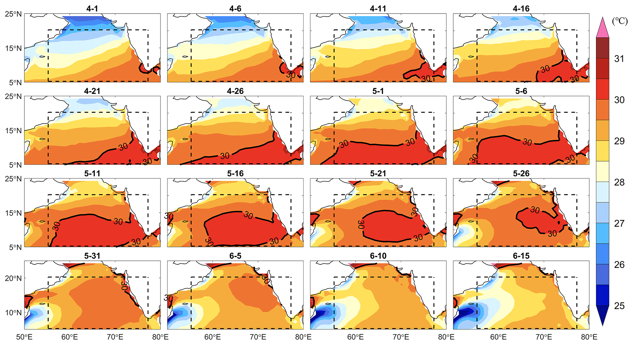
Figure 1 Every 5 d evolution of SST (unit: ^∘C) in April–June, where the black contour is the 30 ^∘C contour. The dashed rectangle represents the selected range of the ASWP (55.25–77.25^∘ E, 5.25–20.25^∘ N). The data are based on a gridded dataset for the period of 1980–2016 from SODA3.7.2 (https://www2.atmos.umd.edu/~ocean/, last access: 5 January 2022).

Figure 2 Time series of the area and maximum temperature of the climatological ASWP, where the blue bars represent the warm-pool area (km²), and the solid line represents the maximum warm-pool temperature (^∘C). The area of the ASWP was the sea area within the rectangular range with a SST greater than 30 ^∘C. The maximum temperature was the highest temperature of the sea area with SST greater than 30 ^∘C within the rectangular sea area.

3.2 ASWP mixed-layer heat budget analysis

To investigate the influence and contribution of different factors during the warm-pool evolution, a mixed-layer heat budget analysis was performed using SODA3.7.2 reanalysis data and JRA-55 heat flux dataset. Throughout the evolution of the ASWP, the sums of SHF, ADV, and ENT were consistent with the trend of mixed-layer temperature. The residual term R was also maintained within 0.1 ^∘C per 5 d, indicating that the heat balance equation was almost closed, and the variation of the ASWP temperature was mainly related to these three terms. Therefore, these three terms can be used to explore the evolutionary mechanism of the ASWP qualitatively and quantitatively (Fig. 3).

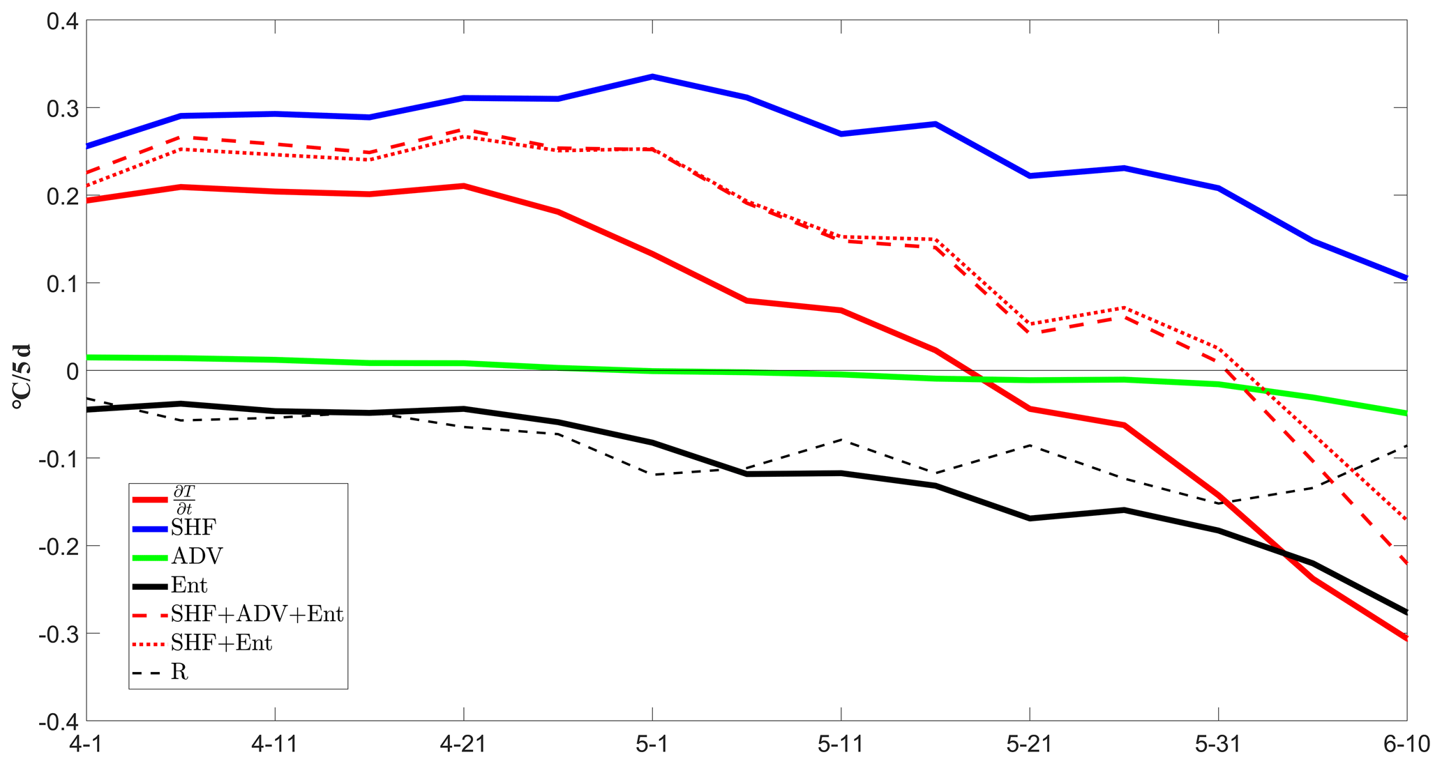
Figure 3 Contribution of different processes to the temperature variation of the warm-pool mixed layer in the AS (^∘C per 5 d), where $\frac{\partial T}{\partial t}$ (solid red line) is the temperature variation of the warm-pool mixed layer with time, SHF (solid blue line) represents the sea surface heat flux forcing, ADV (solid green line) represents the horizontal advection, ENT (solid black line) represents the vertical entrainment, and R (dashed black line) represents the residual. The dashed red line represents the sum of SHF, ADV, and ENT. The dotted red line represents the sum of SHF and ENT.

The variation in the ASWP mixed-layer temperature was asymmetric. From 1 April to 16 May, $\frac{\partial T}{\partial t}$ was greater than zero, and the mixed-layer temperature gradually increased as the ASWP developed. After 21 May, $\frac{\partial T}{\partial t}$ was less than zero, and the mixed-layer temperature rapidly decreased, corresponding to the rapid decay of the warm pool. SHF consistently dominated the warm pool throughout the warming phase, with a contribution of up to 0.34 ^∘C per 5 d. The overall trend of the temperature variation was consistent with SHF. ADV and ENT had less influence on the temperature variation, and the ENT played a weak cooling role. In the cooling phase, the SHF gradually decreased and the ENT strengthened, up to −0.27 ^∘C per 5 d. The effect of ADV was much smaller, not more than 0.1 ^∘C per 5 d. The following is a detailed analysis of the mechanism and effect of each process.

3.2.1 Surface heat flux

The contribution of SHF to $\frac{\partial T}{\partial t}$ ranged from 0.11 ^∘C per 5 d to 0.34 ^∘C per 5 d (Fig. 4), always playing a heating role. From April to early May, the contribution of SHF to temperature was around 0.3 ^∘C per 5 d, indicating that SHF provided substantial thermal support for the increased temperature. By early June, the contribution of SHF to temperature dropped below 0.2 ^∘C per 5 d. The effect of SHF on the warm-pool temperature can be divided into two parts: the net surface heat flux (${\mathrm{SHF}}_{Q_{\mathrm{net}}}$) and the penetrating shortwave radiation at the bottom of the mixed layer (${\mathrm{SHF}}_{Q_{\mathrm{loss}}}$). In the upper layer of the mixed layer, the temperature change is related to the heat exchange between the surface seawater and the atmosphere, so it is related to the net heat flux at the sea surface (${\mathrm{SHF}}_{Q_{\mathrm{net}}}$). In the lower layer of the mixed layer, the heat flux that can penetrate the bottom of the mixed layer is mainly shortwave radiation. Therefore, the heat loss at the bottom of the mixed layer is mainly related to penetrative shortwave radiation (${\mathrm{SHF}}_{Q_{\mathrm{loss}}}$). The contribution of ${\mathrm{SHF}}_{Q_{\mathrm{net}}}$ gradually increased from 0.41 ^∘C per 5 d to 0.50 ^∘C per 5 d in April. It increased slowly but remained at a relatively high level. Then it gradually decreased to less than 0.2 ^∘C per 5 d. Similar to ${\mathrm{SHF}}_{Q_{\mathrm{net}}}$, ${\mathrm{SHF}}_{Q_{\mathrm{loss}}}$ also gradually increased to −0.17 ^∘C per 5 d in April and then decreased.

Figure 4 Contribution of the sea surface heat flux forcing to the mixed-layer temperature (^∘C per 5 d), where blue bars represent the total sea surface heat flux forcing, red bars represent the contribution of the net surface heat flux, and yellow bars represent the contribution of penetrating shortwave radiation at the bottom of the mixed layer.

Figure 5 (a–c) Monthly climatology of shortwave radiation flux (shading; W m⁻²) and mixed-layer temperature (black contours; ^∘C). (d–f) The distribution of total cloud coverage.

${\mathrm{SHF}}_{Q_{\mathrm{net}}}$ is related to sensible heat, latent heat, longwave radiation flux, and shortwave radiation flux (SWR). In climatology, the SWR was the largest contributor (190–283 W m⁻²) and was always positive, indicating that the main source of heat in the warm pool was shortwave radiation from the sun. Therefore, we focused on the variation in SWR in the AS in combination with cloud coverage (Fig. 5). In April, the clear sky and lack of clouds over the AS mean the sea surface can receive more SWR than at other times. The SWR was above 240 W m⁻² throughout the AS, with a clear high value in the center of the AS. In May, when the shortwave radiation flux had decreased (230 W m⁻²), the temperature of the warm pool reached its highest. When the summer monsoon broke out, the atmospheric convective activity was strong and the cloud coverage over the sea was high, leading to a decrease in the shortwave radiation entering the mixed layer. The shortwave radiation dropped to below 220 W m⁻², with a clear low-value center (< 180 W m⁻²) in the southeast of the AS. In addition, although the variation of the mixed-layer temperature was roughly in line with the trend of SWR, the variation of temperature had a lag time of about 1 month compared with SWR. This trend occurred because seawater has a large specific heat capacity, and there is a lag of 1 month in the variation of temperature.

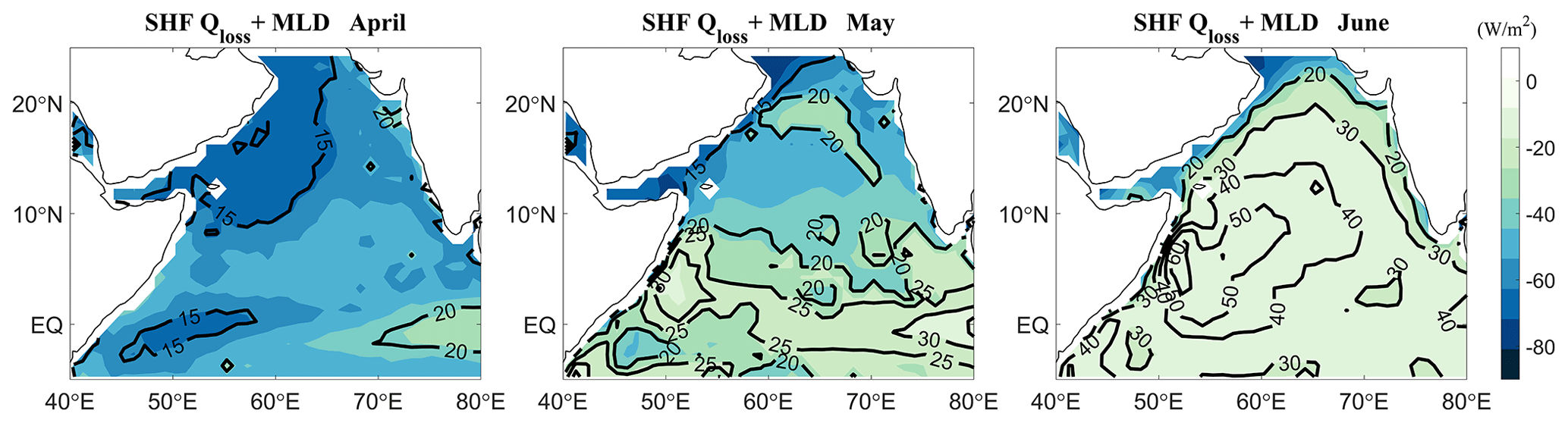
Figure 6 Monthly climatology of shortwave radiation loss penetrating the mixed layer (color shading; W m⁻²) and the depth of the mixed layer (black contours; m).

${\mathrm{SHF}}_{Q_{\mathrm{loss}}}$ was negatively correlated with the mixed-layer depth (Fig. 6). In April, the wind speed over the AS was low, making the mixed-layer depth shallow (< 15 m). Shortwave radiation can penetrate the mixed layer at this time (−55 W m⁻²) and heat the subsurface seawater. In May, when the summer monsoon was about to onset, increased wind strengthened the ocean mixing, leading to a deeper mixed layer (25 m) and a decrease in the shortwave radiation penetrating the mixed layer (−37 W m⁻²). In June, when the summer monsoon was fully formed, the mixed layer was further deepened (> 30 m), and the penetrating shortwave radiation through the mixed layer was further decreased (−9 W m⁻²). In addition, the study by Liu and Chu (2007) found that the mixed layer depth is forced by penetrative shortwave radiation, and the impact of penetrative shortwave radiation on the depth of the mixed layer is controlled by wind speed and net shortwave radiation at the sea surface.

3.2.2 Vertical entrainment

The contribution of ENT to temperature ranged from −0.04 ^∘C per 5 d to −0.28 ^∘C per 5 d (Fig. 7), acting as a cooling effect and intensifying over time. Together with the gradual decrease in SHF, it led to a rapid cooling of the ASWP. During the development phase of the warm pool, the cooling effect of ENT was weak, accounting for only 16 %–20 %. After 1 May, the cooling effect intensified up to 58 %. The effect of ENT on temperature can be divided into three parts: the entrainment due to the vertical velocity (ENT1), the entrainment due to the local tendency of the mixed-layer depth (ENT2), and the entrainment due to “advection of the mixed-layer depth” (ENT3). The cooling effect due to the local variation of the mixed layer was the strongest and almost dominated, ranging from −0.05 ^∘C per 5 d to −0.18 ^∘C per 5 d (Fig. 8).

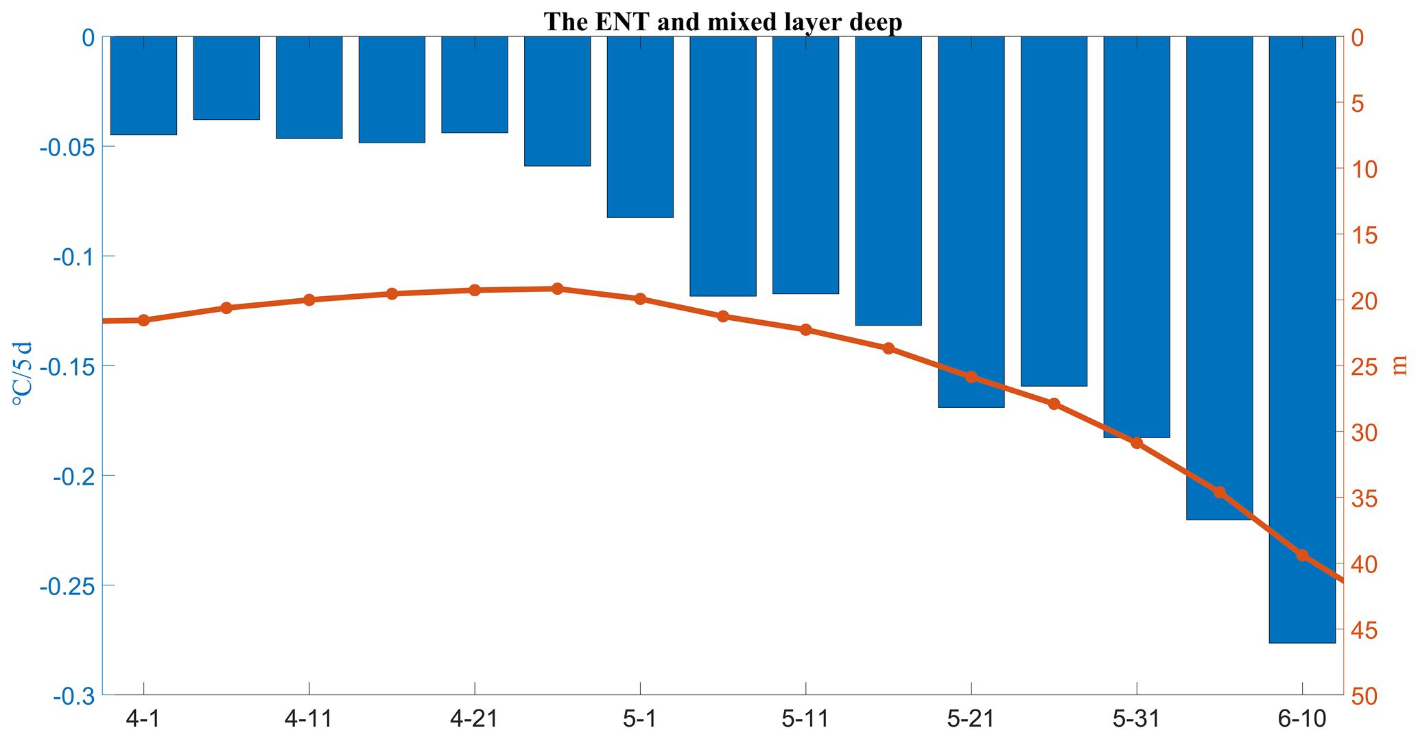
Figure 7 Variation of the vertical entrainment and mixed-layer depth, where the blue bars represent the vertical entrainment (^∘C per 5 d), and the red line represents the mixed-layer depth (m).

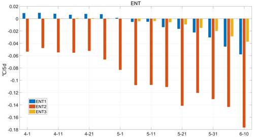
Figure 8 Contribution of each term in the vertical entrainment to the temperature change of the mixed layer.

The vertical entrainment is closely related to the vertical thermohaline structure of seawater and the depth of the mixed layer. When the mixing of the upper seawater in terms of temperature and salinity is inconsistent, the isothermal layer and mixed layer will differ, and a barrier layer will be formed between the bottom of the mixed layer and the top of the thermocline (Sprintall and Tomczak, 1992). The barrier layer has the characteristics of a strong salinity gradient and high gravitational stability, which makes it difficult to transport heat from top to bottom by mixing. On the one hand, a strong and stable salinity stratification can effectively inhibit the transfer of non-shortwave radiation flux to the interior of the ocean, which leads to the warming of the upper mixed layer. On the other hand, the existence of the barrier layer can inhibit the entry of the cold water of the thermocline into the mixed layer, which is not conducive to the exchange of heat, momentum, mass, and nutrients between the mixed layer and the thermocline (Pang et al., 2021). Therefore, In the development stage of the ASWP, the low wind speed made the mixed-layer shallower, which made the seawater within the mixed layer more easily heated and thus more sensitive to heat flux. Then the weak wind speed and the existence of anticyclonic circulation (Shankar et al., 2002) associated with the Lakshadweep High trapped the fresh water, contributing to the formation of the barrier layer, maintaining the ASWP by effectively inhibiting the vertical mixing of the upper ocean and causing the warming of the upper mixed layer. In the late stage of ASWP evolution, with the imminent onset of the summer monsoon, the stirring effect of wind started to strengthen, the mixing layer became deeper rapidly (Fig. 6), and the cooling effect of entrainment was enhanced, which accelerated the decay of the ASWP (Liu et al., 2013).

3.2.3 Horizontal advection

The contribution of ADV to $\frac{\partial T}{\partial t}$ ranges from −0.05 ^∘C per 5 d to 0.01 ^∘C per 5 d, which is much smaller than the contribution of other processes. From 1 April to 1 May, the contribution of ADV was positive, indicating that the advection process played a weak heating role during the development phase. After 1 May, ADV started to become negative and played an increasingly important cooling role in the warm pool. Due to heavy rainfall and river runoff over evaporation, the salinity of the seawater in the Bay of Bengal was very low. During November and December, there is an equatorward-flowing East India Coastal Current (EICC) off the east coast of India. This current flows around Sri Lanka and continues as a poleward-flowing West India Coastal Current off the west coast of India (Shetye et al., 1996; Rao and Sivakumar, 1999; Mukhopadhyay et al., 2020). The EICC carries a large amount of low-salt seawater from the Bay of Bengal into the AS. This coastal current system is further strengthened between December and February by the westward North Equatorial Current (NEC). These low-saline waters create a near-surface halocline, which enhances stratification. Then the stratification prevents the vertical redistribution of the turbulent and radiative heat fluxes, amplifying the change in SST (Rao and Sivakumar, 1999). Due to the low wind speed in the AS from April to May, the sea surface flow field is very weak. Coupled with the anticyclonic circulation (Shankar et al., 2002) associated with the Lakshadweep High (Bruce et al., 1994), the low-salinity water is trapped in the AS and can be maintained until May, promoting the formation of the barrier layer, which is conducive to the development and maintenance of the ASWP. In June, the summer monsoon is about to break out, the sea surface wind field changes, the sea surface flow field also turns, and the salinity stratification weakens, promoting the disappearance of the ASWP.

Therefore, during the development and peak stages of the ASWP, strong shortwave radiation flux causes sea temperature to continuously rise, gradually forming a warm pool. The presence of weak wind and the barrier layer allows for the maintenance of high temperature. During this time, the ASWP is mainly influenced by the sea surface heat flux forcing, with little impact from vertical entrainment and horizontal advection. In the decline stage of the ASWP, the rapid decrease in shortwave radiation flux weakens the heating effect of the sea surface heat flux forcing, while the strengthening of mixing leads to an increase in vertical cooling. The combined effect of these two factors results in a sharp decrease in temperature, leading to the rapid decline of the warm pool.

4 Interannual variability of the ASWP

4.1 Characteristics of the interannual variability of ASWP

The ASWP does not occur every year; its intensity and extent vary from year to year. As shown in Fig. 9, there has been a significant interannual variation in the area of the ASWP. The ASWP was a large area in 1980, 1991, 1998, 2003, 2005, 2010, 2014, 2015, and 2016, exceeding 0.5 standard deviations of the area and reaching a maximum of 3.1×10⁶ km². In other years, the area of the warm pool has been almost negligible (1984, 1989, 1992, 1999, 2000, 2008), indicating that the ASWP is weak in these years. A basin-scale warming/cooling is the leading mode of tropical Indian Ocean SST variability on interannual timescales. It peaks in late winter and persists into the following spring and summer (Klein et al., 1999; Li et al., 2008). The years with a large (small) ASWP area correspond to positive (negative) IOB periods, indicating that the ASWP area is mainly controlled by IOB (Guo et al., 2018).

Figure 9 Time series of ASWP area from April to June 1980–2016 (the area calculated is daily mean every 5 d; red dots indicate the average area of ASWP per year). The horizontal black continuous line represents the seasonal mean, and the dashed lines represent ±0.5 standard deviations.

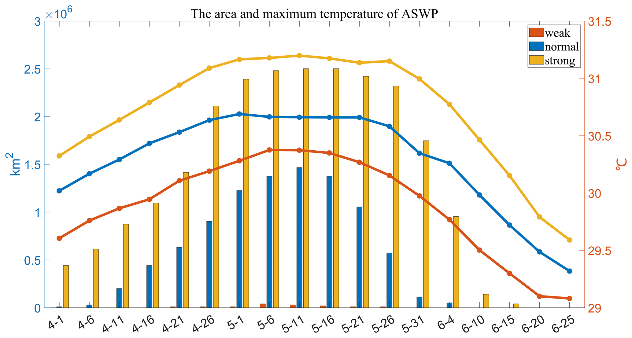
Figure 10 Variation of the area and maximum temperature of different types of ASWP (calculated every 5 d), where the bars represent the area of the warm pool (km²), the solid lines represent the maximum temperature of the warm pool (^∘C), red line represents those during a weak ASWP, blue represents those during a normal ASWP, and yellow represents those during a strong ASWP.

Figure 11 ASWP mixed-layer heat budget diagnosis, with weak ASWP years on the left, normal ASWP years in the middle, and strong ASWP years on the right.

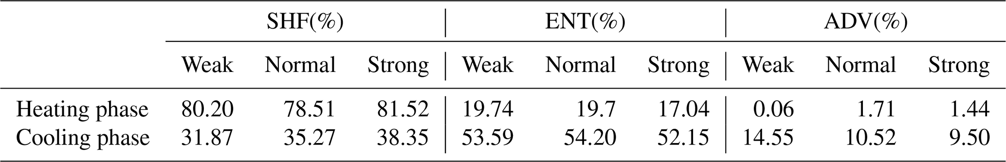
Based on a 0.5σ criterion, we estimated the average area of the ASWP for each year and identified the weak, normal, and strong ASWP years. As shown in Figs. 10 and 11, the warm-pool area and maximum temperature were always the highest in strong ASWP years, with an average area of 1.3×10⁶ km² and a maximum temperature of 30.7 ^∘C. In normal years, the average area was 0.53×10⁶ km², and the maximum temperature was 30.3 ^∘C. In weak ASWP years, the average area was only 7.8×10³ km², and the maximum temperature was only 29.9 ^∘C. The diagnostic results of its mixed layer synthesized separately indicated similarity to the diagnostic results of the climatology (Fig. 3). During the warming phase, the temperature changes were faster in strong ASWP years (> 0.2 ^∘C per 5 d), while the temperature changes were smaller in weak ASWP years (< 0.2 ^∘C per 5 d). This is consistent with the faster expansion and larger area of ASWP in strong years. However, regardless of the year, the contribution of SHF to the temperature change was largest (78.5 % to 81.5 %), and the contributions of ENT and ADV were relatively small (Table 1). Among them, the weaker warm pool in weak ASWP years may be related to the greater cooling effect of ENT at this time (19.7 %). In the cooling phase, the contribution of SHF decreased (31.9 % to 38.3 %), the cooling effect of ENT increased (52.2 % to 54.2 %), and the contribution of ADV increased slightly (9.5 % to 14.6 %). SHF and ENT together dominated the temperature change of the ASWP. The larger (smaller) warm pool in strong (weak) ASWP years may be related to the larger (smaller) heating effect of SHF and the smaller (larger) cooling effect of ENT and ADV.

Table 1 Contribution of each term to temperature variation.

4.2 The relationship between ASWP and IOD/ENSO

The EOF analysis was conducted separately for temperatures in the AS from April to June by using SST anomaly from the SODA3.7.2 dataset, and the first two modes were used for the analysis (Fig. 12). In April, May, and June, the variance contributions of the first mode were all greater than 50 % (60.86 %, 54.80 %, and 51.83 %). The spatial distributions were similar, showing a consistent change of the temperature in the AS. This was mainly related to the Indian Ocean basin model (Guo et al., 2018). The principal component (PC) time series in April and May showed large positive peaks in 1987, 1991, 1998, 2010, and 2016, indicating that the temperature in April and May in the AS was anomalously warm in these 5 years. This corresponds to several years with large ASWP areas, indicating that the large ASWP ranges in these 5 years were mostly due to the consistent warming of the IOB. Similarly, the years with negative peaks in the PC time series (1989, 1992, 1999, 2000, and 2008) coincide with the years with smaller ASWP areas, suggesting that these 5 years with smaller ASWP ranges were controlled by the IOB. The variance contribution of the second mode (10.71 %, 12.51 %, and 11.52 %) was much smaller than the first mode. The spatial distribution pattern varied by months, but there are at least two antiphase extreme centers.

Figure 12 EOF1 (the first column), EOF2 (the second column), and PC1 and PC2 (the third column) of SST anomalies in the AS for April–June.

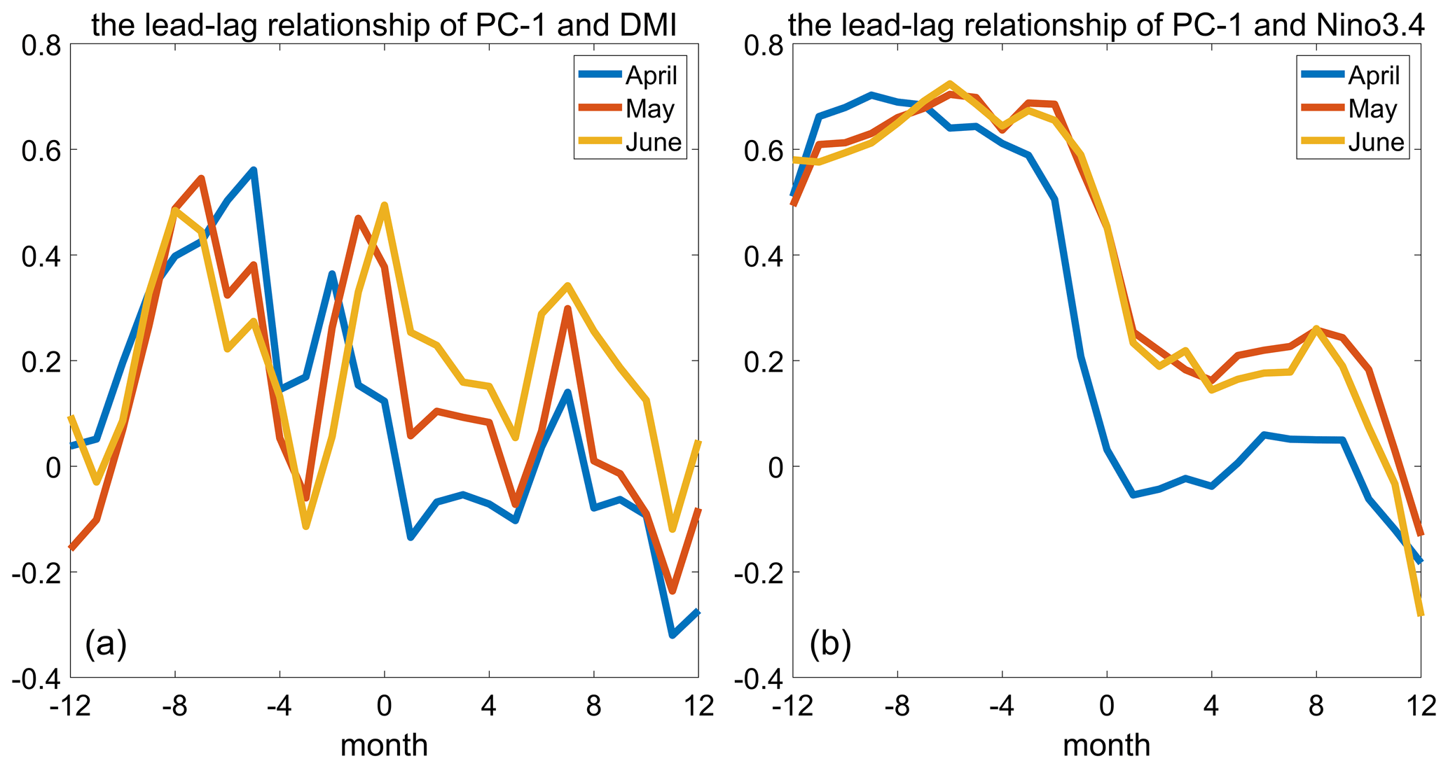
Figure 13 Lead–lag correlation between PC1 and the IOD index DMI (a) and ENSO index Niño3.4 (b) in April, May, and June.

The most dominant interannual climate modes in the TIO are the IOB mode and the IOD mode (Schott et al., 2009). Therefore, we further investigated the effects of IOB and IOD on the interannual variability of the ASWP. When the IOB is in a positive phase, there is consistent warming across the AS with a large range and intensity in the ASWP. This is consistent with ASWP's larger area in 1987, 1991, 1998, 2005, 2010, 2014, 2015, and 2016. The IOD is an inherent interannual climate mode in the TIO. During a positive phase, warm waters are pushed to the western part of the Indian Ocean, while cold deep waters are brought up to the surface in the eastern Indian Ocean. This pattern is reversed during the negative phase of the IOD (Saji et al., 1999; Kumar et al., 2020). The AS is located in the western side of the Indian Ocean, which is part of the western IOD. Its local sea–air interaction and interannual variation are closely related to the IOD. The left panel of Fig. 13 shows that the highest correlation coefficient between the PC1 and IOD reached 0.56 (p < 0.01), indicating that the ASWP had a significant correlation with the IOD. There are three peaks in the lead–lag correlation between PC1 and IOD. The first peak appears at −5, −7, and −8 months (r= 0.48–0.56), indicating that the correlation is highest when the sea temperature lags the IOD 5–8 months; this is consistent with the IOD peaks in winter (Li et al., 2008). The second peak appears at −2, −1, and 0 months (r= 0.36–0.49), indicating that the IOD can also regulate the temperature in near-real time. The third peak appears at 7 months (r= 0.14–0.34), indicating that the temperature is not only regulated by IOD, but can also affect the IOD mode, although the effect is relatively small. This is consistent with the research results of Li et al. (2008). The Indian Ocean is directly and indirectly influenced by global or other regional climate patterns, such as the ENSO. Therefore, we also considered the impact of the ENSO on the interannual variability of the ASWP. Previous research has indicated that the ENSO has an impact on SST over the Indian Ocean (Klein et al., 1999; Thandlam et al., 2020). Both observations and model studies indicate that the Indian Ocean warms (cools) throughout the ocean basin in March–May following an El Niño (La Niña) year (Song et al., 2007; Dommenget and Jansen, 2009; Venugopal et al., 2018; Thandlam et al., 2023). Kim et al. (2012) investigated the warm-pool features in the Indian and Pacific oceans and discovered that the seasonal variations in the Indian Ocean were greater than in the Pacific, which was due mostly to ENSO. The intensity of the warm pool was associated with a 5–6-month delay after the ENSO. The right panel of Fig. 13 shows the lead–lag correlation between the PC1 of ASWP and Niño3.4. The correlation coefficient between PC1 and the Niño3.4 index is highest at a lag of 5–7 months (r= 0.61–0.72) and then sharply decreases after −2 months. This indicates that the temperature is modulated by the ENSO. In other words, after the El Niño (La Niña) peaks in winter, the ASWP before the summer monsoon in the upcoming year was more (less) pronounced, which is consistent with the strength of the IOWP peaking about 5 months after the ENSO peaked. This delay is because that the ENSO-induced teleconnection between oceans takes some time to develop (Lau and Nath, 2003). ENSO can not only directly affect the temperature changes in the AS through atmospheric bridges (Lau and Nath, 2000; Chowdary and Gnanaseelan, 2007), but also indirectly regulate the temperature changes by influencing the IOD (Behera et al., 2006). So, the correlation coefficient between the ENSO index and PC1 is higher than that of IOD, and the impact is stronger.

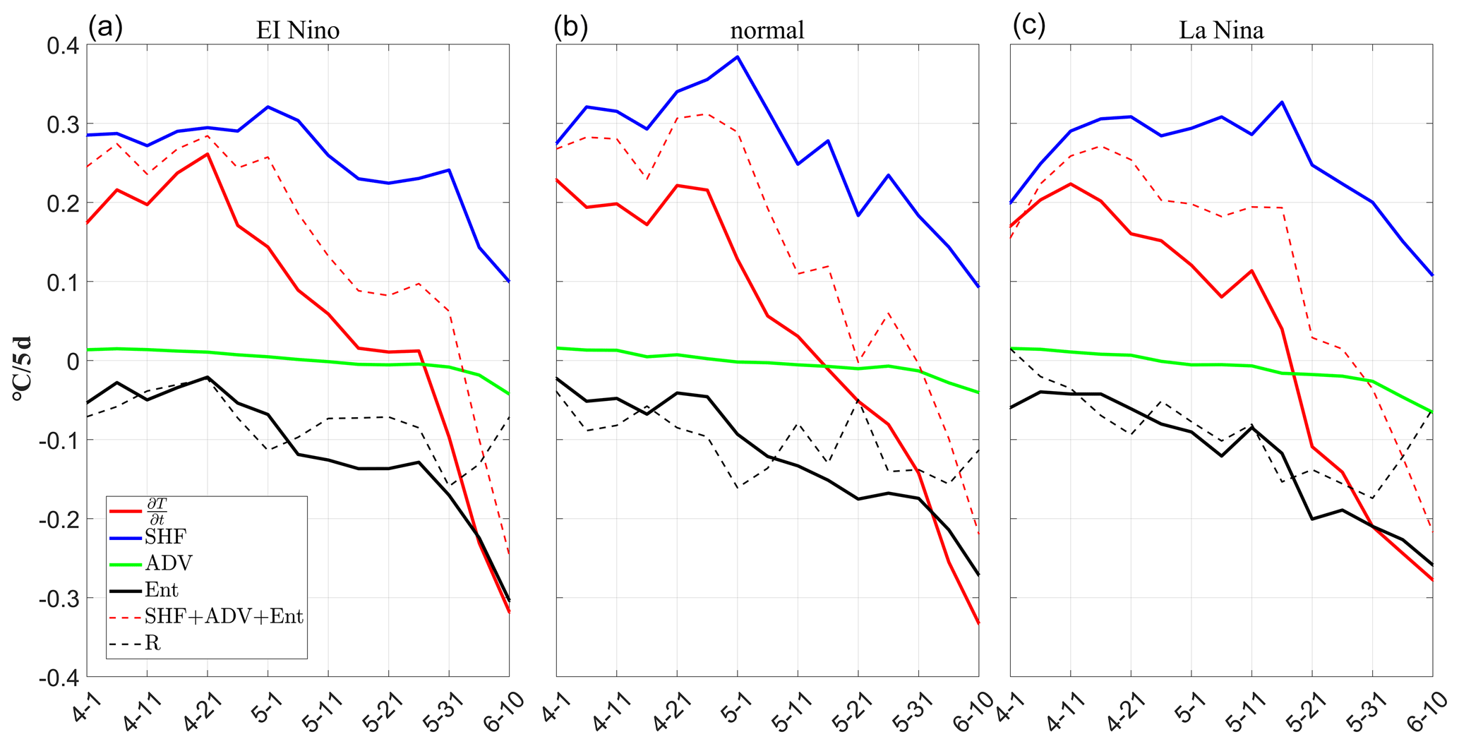
Figure 14 ASWP mixed-layer heat budget with El Niño year (a), normal year (b), and La Niña year (c).

Can changes in the ENSO affect the role of different processes in the evolution of the ASWP? To explore this question, we divided the ASWP into El Niño, La Niña, and normal years and diagnosed them separately. The results are shown in Fig. 14. It can be seen from the overall trend that the change in the ENSO did not change the dominance of SHF and ENT in the evolution of ASWP. However, the surface heat flux forcing still dominated in the warming phase, and the surface heat flux and the vertical entrainment together dominated the temperature change of ASWP in the cooling phase. It is noteworthy that although the temperature warmed up during El Niño, the effect of surface heat flux forcing did not increase significantly. However, the effect of vertical entrainment was enhanced, which may be related to the enhanced convective activity and mixing effect during El Niño (Sullivan et al., 2019).

5 Summary and discussion

In this study, we analyzed the causes of the Intraseasonal variability in the ASWP using heat budget analysis and explored the relationship between the interannual variability of the ASWP and large-scale modes using lead–lag correlation. By using the latest 5 d SODA reanalysis dataset, we found that the formation and extinction of the ASWP were completed in April, May, and June. Its formation and decay rates showed asymmetry, with a decay rate twice as fast as the development rate.

The results of the heat budget analysis show that the sea surface heat flux forcing had the largest effect on the ASWP's mixed-layer temperature. The next most important factor was the vertical entrainment, and then the horizontal advection had the smallest effect, which is consistent with previous results. The effect of SHF on the warm-pool temperature was divided into two parts,${\mathrm{SHF}}_{Q_{\mathrm{net}}}$ and ${\mathrm{SHF}}_{Q_{\mathrm{loss}}}$. ${\mathrm{SHF}}_{Q_{\mathrm{net}}}$ was mainly related to shortwave radiation, which is at a maximum in April due to the lack of clouds and gradually decreases with an increase in cloudiness in May and June. ${\mathrm{SHF}}_{Q_{\mathrm{loss}}}$ was related to the depth of the mixed layer and increases with the onset of the summer monsoon in June. The ENT always played a cooling role. The increasing cooling effect made the ASWP decay rapidly, and the effect due to the local changes in the mixed layer was the strongest.

ASWP, as part of the Indian Ocean, has strong interannual variability. The diagnostic analysis revealed that, during the warming phase, temperature changes were faster in strong ASWP years. While the temperature changes were smaller in weak ASWP years. This is consistent with the faster expansion and larger area of the ASWP in strong years. Then we found that the ASWP had a positive correlation (r= 0.56) between its PC1 and IOD most of the time. Concerning the ENSO, the ASWP had the largest correlation at a lag of 5–7 months for the Niño3.4 index, showing that it was modulated by the ENSO. In other words, after the El Niño (La Niña) peaks in winter, the ASWP before the summer monsoon in the upcoming year was more (less) pronounced.

However, there are many interacting factors affecting the variability of temperature in AS. In this paper, we investigated the effects of only three processes: sea surface heat flux forcing, horizontal advection, and vertical entrainment. We did not consider other factors, such as horizontal and vertical diffusion, which require further optimization of the diagnostic formula and more comprehensive diagnostic methods. In addition, the variation of ASWP is influenced by various global-scale modes. Its development, extinction, and interannual variation should be regarded as a coupled ocean–land–air process. In this way, we can capture its variation characteristics, dynamic mechanisms, and influence on various sea–air interaction processes more comprehensively and accurately.