Spatial and temporal variability in mode-1 and mode-2 internal solitary waves from MODIS-Terra sun glint off the Amazon shelf

The Amazon shelf is a key region for intense internal tides (ITs) and nonlinear internal solitary wave (ISWs) generation associated with them. The region shows well-marked seasonal variability (from March to July, MAMJJ, and from August to December, ASOND) of the circulation and stratification, which can both induce changes in the ISW physical characteristics. The description of the seasonal and neap–spring tidal variability in the ISWs off the Amazon shelf is performed for the first time using a meaningful data set composed of 140 MODIS-Terra imagery from 2005 to 2021, where about 500 ISW signatures were identified in the sun glint region. Previous studies have documented the existence of mode-1 ISWs, but the region appears as a newly described hotspot for mode-2 ISWs. ISW packets separated by typical mode-1 (95–170 km; 2.1–3.8 m s⁻¹) and mode-2 (46–85 km; 1.0–1.9 m s⁻¹) IT wavelengths have been identified and mapped coming from different IT generation sites. For each ISW, a group of waves (3 to 10) is generally follows the largest crest. The intra-packet distance between each wave in the group is about 10 to 20 km. Regions of higher occurrence of ISWs are spaced by a IT mode-1 wavelength. We make the assumption that it might correspond to the IT reflection beams at the surface, which may generate newer ISWs. The mean mode-1 and mode-2 inter-packet distances do not show significant differences according to their IT generation sites. The ISW activity is higher (more than 60 % of signatures) during spring tides than neap tides. In the region under the influence of the North Equatorial Counter Current (NECC), ISWs are separated by a mean mode-1 IT wavelength which is 14.3 % higher during ASOND than during MAMJJ due to a deeper thermocline and the reinforcement of the NECC. These ISWs are also characterized by a wider inter-packet distance distribution (higher standard deviation) that may be related to the stronger eddy kinetic energy (EKE) during ASOND compared to MAMJJ. The mean inter-packet distance of mode-2 ISWs remains almost unchanged during the two seasons, but the inter-packet distance distribution is wider in ASOND than in MAMJJ as for mode 1. Note that these results need to be treated with caution, as only few occurrences of mode-2 waves were found during MAMJJ. In the region of the NECC, the direction of propagation for all modes is very similar in MAMJJ (about 30^∘ clockwise from the north), whereas, for ASOND, the ISWs propagate in a wider pathway (from 0 to 60^∘ clockwise from the north), due to a much larger eddy activity. During ASOND, as the background flux goes further east, the inter-packet distances become larger (4 % for mode 1 and 7.8 % for mode 2). These results show that the reinforcement of the NECC in ASOND appears to play a role in diverting the waves towards the east, increasing their phase velocities and their eastern traveling direction component when compared to MAMJJ. Calculations of the IT velocities using the Taylor–Goldstein equation supported our results regarding the presence of ISWs associated with mode-2 ITs and additionally the IT seasonal variability.

1 Introduction

Nonlinear internal solitary waves (ISWs) are generated in the ocean by various processes, including the interaction of the flow with underwater sills/banks, and the evolution and disintegration of internal tides (ITs) (Jackson et al., 2012; Alford et al., 2015). Their turbulent mixing and strong horizontal and vertical currents have an impact on oceanic physical and biological processes (e.g., redistribution of heat, momentum across oceanic basins, and nutrient supply for photosynthesis) (Sandstrom and Elliott, 1984; Huthnance, 1995; Munk and Wunsch, 1998; Muacho et al., 2013), while ISW can also represent a source of hazards for economic activities (e.g., aquaculture and offshore drilling operations) (Osborne et al., 1978; Hyder et al., 2005).

The Amazon shelf has been reported in the literature as being an important hotspot for intense IT and ISW generation (Brandt et al., 2002; Magalhães et al., 2016; Lentini et al., 2016; Bai et al., 2021; Tchilibou et al., 2022). Different work has already documented the presence of ISWs on the Amazon shelf, with studies illustrating their propagation both offshore (Brandt et al., 2002; Magalhães et al., 2016) and along the continental shelf (Lentini et al., 2016; Bai et al., 2021). The former is associated with IT hotspots over the steep slopes of the Amazon shelf break and disintegration into short-scale waves several hundred kilometers from the shelf break (Magalhães et al., 2016). The shorter-scale ISWs are trapped in the IT troughs, both propagating together (Jackson et al., 2012). Magalhães et al. (2016) identified two regions (called A and B) as being the most energetic generation sites (see their Fig. 1). In Tchilibou et al. (2022), more than six sites of internal-tide generation were identified along with the Amazon shelf break, sites A and B remaining the strongest.

Intra-seasonal to seasonal variability in the circulation and stratification and neap–spring tidal forcing is linked to changes in the IT and ISW propagation direction, intensity, horizontal scales, and, consequently, velocities (Vlasenko et al., 2012; Magalhães et al., 2016; Liu and D’Sa, 2019; Tchilibou et al., 2022). The Amazon shelf is characterized by two seasons with well-marked differences in water stratification, surface currents, and mesoscale circulation. From March to July, hereafter MAMJJ, the currents and mesoscale activities are weaker and the pycnocline is shallower, slightly stronger, and horizontally more homogeneous; from August to December, hereafter ASOND, the currents and mesoscale activity are intensified and the pycnocline is deeper and slightly weaker and has a stronger horizontal gradient along with the North Brazil Current retroflection and North Equatorial Countercurrent (NBCR-NECC) path (Richardson and Walsh, 1986; Richardson et al., 1994; Silva et al., 2005; Aguedjou et al., 2019; Tchilibou et al., 2022). Seasonal variability in the ISWs in the region was linked to the seasonality of the NECC, which was identified as the mechanism responsible for refracting the waves toward the east and enhancing their velocities during the ASOND time period (Magalhães et al., 2016). The seasonality of the pycnocline depth and strength was linked on the Amazon shelf to changes in the IT baroclinic mode and wavelength (Barbot et al., 2021; Tchilibou et al., 2022). Finally, the currents may interact with the IT field creating some refraction, branching, or even dissipation of the tidal baroclinic flux (Dunphy et al., 2017; Tchilibou et al., 2022). During ASOND, Tchilibou et al. (2022), in a realistic regional modeling configuration, showed that the eddy kinetic energy is higher and the mesoscale currents create a more energetic non-coherent baroclinic flux. This study further illustrated that the latter flux has numerous branches and deviations, and the internal-tide field seems more diffuse. The impact of the water stratification and the seasonal variability was also discussed for mode-2 ITs off the Amazon shelf by Barbot et al. (2021) and Tchilibou et al. (2022). Analyzing the vertical modal structure for mode-2 IT, a deeper pycnocline seems to shift the extrema of the modes toward intermediate water layers (i.e., the first extremum is deeper and the second one is shallower), decreasing the IT elevation amplitude and increasing its horizontal surface wavelength (with a lower impact on mode 2 than on mode 1) (Barbot et al., 2021). During MAMJJ, the shallower and slightly stronger pycnocline seems to enhance the generation of higher baroclinic-mode ITs, enhancing the local dissipation (Tchilibou et al., 2022).

In that study area, Magalhães et al. (2016) found ISWs with an average inter-packet distance with typical wavelengths of long (semi-diurnal) ITs of the fundamental mode (i.e., mode-1 ITs). However, the presence of small-scale ISWs with an average inter-packet distance with the typical wavelength of mode-2 ITs was briefly reported in the region by da Silva et al. (2016). The authors called these smaller-scale features as wave tails. Signatures of small-scale ISWs trailing larger ISWs have been documented in the South China Sea, the Mascarene Ridge of the Indian Ocean, and the Andaman Sea (Guo et al., 2012; da Silva et al., 2015; Magalhães and da Silva, 2018). In the South China Sea, simulations showed two different processes leading to short internal waves riding on mode-2 ISWs and following a strong mode-1 ISW. The first one is related to the disintegration of a baroclinic bore, which is generated by the interaction between topography and tidal current. The second process calls for nonlinear interaction between mode-1 and mode-2 ISWs, which takes place when a faster mode-1 wave overtakes a mode-2 ISW generated one tidal cycle earlier (Guo et al., 2012). In the Mascarene Ridge and the Andaman Sea, the impact of the ISW beam with the pycnocline is identified as the mechanism responsible for the generation of mode-2 ISWs subsequently developing shorter-scale waves (wave tails with mode-1 structure) (da Silva et al., 2015; Magalhães and da Silva, 2018). Potential mechanisms for the generation of mode-2 waves have been illustrated and they include the instability of shoaling mode-1 waves (Helfrich and Melville, 1986) and their interaction with localized sills (Lamb and Warn-Varnas, 2015), the propagation of mode-1 waves into a horizontally varying stratification regime (Liang et al., 2018), and shoaling mode-2 semi-diurnal internal tides (Liang and Li, 2019). The mode-2 waves receive less attention in the literature compared to mode 1, although some works document mode-2 waves propagating with a mode-1 tail in Knight Inlet, British Columbia (Farmer and Smith, 1980) and/or illustrate their occurrence following mode-1 waves in the South China Sea (Yang et al., 2009; Liu et al., 2013).

Remote sensing (RS) is a key observation tool for providing new insights into the ISW generation, propagation, and dissipation mechanisms. Research efforts concerning ISWs are often based on synthetic aperture radar (SAR) and on optical images acquired under sun glint conditions (i.e., areas where the sunlight suffers from specular or near-specular reflection directly onto the sensor viewing angle) (Jackson and Alpers, 2010; da Silva et al., 2011; Liu et al., 2014; Magalhães et al., 2016). Signatures of oceanic features on sun glint imagery are produced by variations in short-scale sea surface roughness which cause changes in the image glitter brightness (Jackson and Alpers, 2010; Kudryavtsev et al., 2012). Since ISWs produce leading bands of rough followed by smooth sea surface associated, respectively, with convergent and divergent surface currents, this oceanic feature can be observed in sun glint imagery (Alpers, 1985; Jackson and Alpers, 2010).

Here, we study the ISWs off the Amazon shelf using for the first time a comprehensive data set composed of 140 images acquired by the Moderate Resolution Imaging Spectroradiometer (MODIS) onboard the Terra satellite (January 2005 to December 2021). ISWs with an inter-packet distance with typical wavelengths of mode-1 and mode-2 ITs have been mapped and their propagation velocities and directions are analyzed, considering their seasonal and neap–spring tidal variability. Calculations of the IT phase velocities using the Taylor–Goldstein equation (TGE) supported our results regarding the presence of shorter-scale ISW tails separated by mode-2 IT wavelengths in the study area and additionally the IT seasonal variability. For the first time, the Amazon shelf is described as an important hotspot for shorter-scale ISWs coupled with mode-2 ITs.

2 Data and methods

2.1 Remote-sensing and reanalysis data

The RS data set is composed of 140 images (acquired from 1 January 2005 to 31 December 2021) of Level 1B data from the MODIS sensor onboard the Terra satellite. The images were acquired off the Amazon shelf, where the presence of ISW signatures was identified in the sun glint region using band 6 centered at 1640 nm with a spatial resolution of 500 m. Level 1B MODIS-Terra images were collected from NASA's Earth Science Data System (ESDS) (MODIS-Terra, https://doi.org/10.5067/MODIS/MOD02QKM.NRT.061). The cloud coverage (especially during the months of MAMJJ) and the position of the sun glint area, which changes over the year, are limiting factors for our samples.

The Global Ocean Ensemble Physics Reanalysis (EPR, https://doi.org/10.48670/moi-00024) data provide a 3D-gridded description of the global oceanic physical state at 0.25^∘ resolution, from January 1993 to December 2019. The data are produced by Mercator Ocean International as part of the Copernicus Programme (https://marine.copernicus.eu/, last access: 4 March 2022), using a multi-numerical ocean model (GLORYS2V4 from Mercator Ocean, France; ORAS5 from the ECMWF; GloSea5 from the Met Office, United Kingdom; and C-GLORSv7 from CMCC, Italy) ensemble approach and data assimilation of satellite and in situ observations. The daily mean average of temperature, salinity, and current variables was acquired from 2005 to 2019 for 75 vertical levels.

2.2 Remote-sensing data processing

The ISW signatures were visually identified and manually extracted for each MODIS-Terra scene of our data set. Signatures of nonlinear ISWs can be visualized as leading bands of increased sea surface roughness followed by bands of decreased roughness (Alpers, 1985; Jackson and Alpers, 2010). The leading wave of each ISW packet was mapped for each image of our data set, and the distance between two consecutive leading wave signatures (inter-packet distance) was calculated considering the vector which connects the middle point of each consecutive ISW signature, perpendicular to the ISW crests. The ISW inter-packet distances can be used as a proxy for the IT wavelengths. An image showing a typical view of this study region, in which it can be seen that ISW signatures are often found with typical mode-1 and mode-2 IT wavelengths (hereafter called mode-1 and mode-2 ISWs), can be seen in Fig. 1. The average wave propagation velocity was calculated considering the period of the semi-diurnal IT of 12.42 h. The ISW propagation direction was automatically retrieved from the RS data considering the angle between the north and the direction of the vector which connects the middle point of two consecutive packets (in a clockwise direction); i.e., $pd=\mathrm{0}{}^{\circ }$ means ISWs propagating from the south to the north, and $pd=\mathrm{90}{}^{\circ }$ means ISWs propagating from west to east.

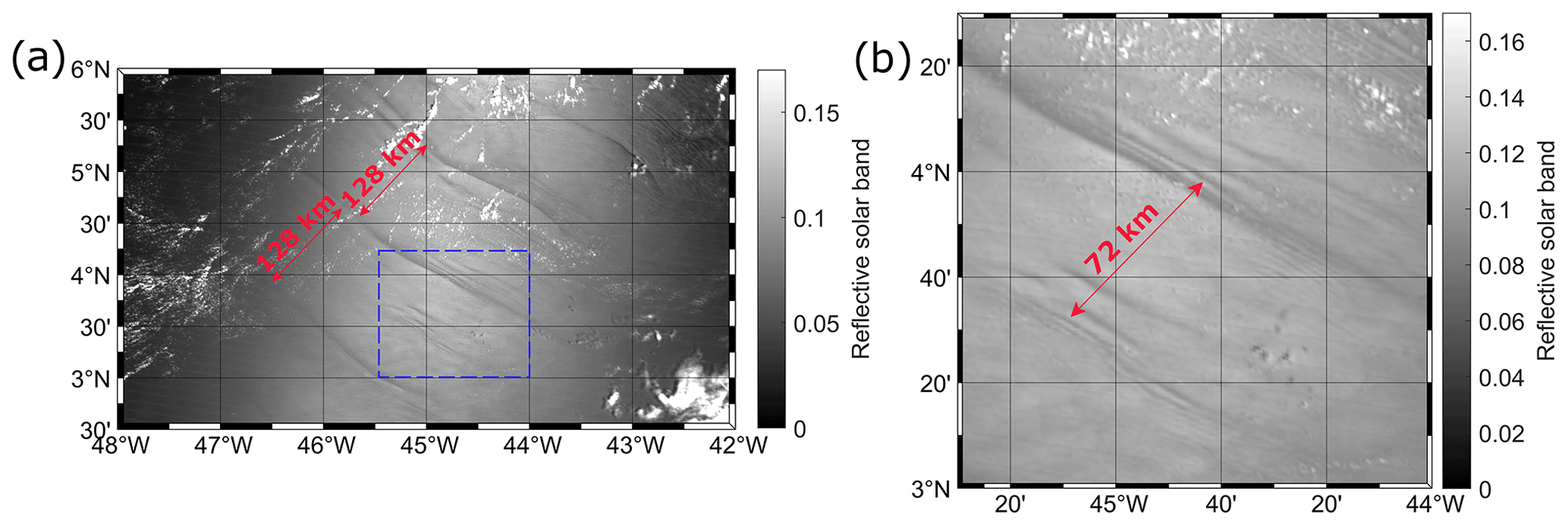
Figure 1 Level 1B MODIS-Terra image, band 6, acquired on 10 October 2014 shows (a) a typical view of this study region, in which it can be seen that ISW signatures are often found with typical mode-1 IT wavelengths. The blue rectangle represents the area where (b) signatures associated with mode-2 ITs are found.

2.3 Theoretical calculation of IT velocities

The wave velocities of all modes are calculated using inviscid solutions of the TGE, following the method proposed by Lian et al. (2020). The Coriolis force due to the Earth's rotation is not taken into account by Lian et al.'s method. However, in our study area, this effect can be neglected due to the proximity to the Equator. The approach is used to support the existence of mode-2 IT waves off the Amazon shelf, including the understanding of the wave's seasonal and near-spring tide variability in terms of shear and water stratification. The local values of stratification and shear were taken from daily and monthly EPR data for each location where ISWs were identified considering the entire period of time (from 2005 to 2019). The current velocities were decomposed in the ISW traveling direction. Here, positive velocity means current flowing in the same direction as the ISWs/IT, while a negative one means current flowing in the opposite direction. The separation between the different wave modes is based on the probability distribution of the velocities predicted by the viscous TGE for mode 1 and mode 2, considering the monthly EPR data. It is important to point out that the underestimation of the ISW phase velocity calculated using the TGE is expected since the equation calculates linear wave phase speed and the nonlinear effects increase the speed of the linear waves (Alford et al., 2010; da Silva et al., 2011).

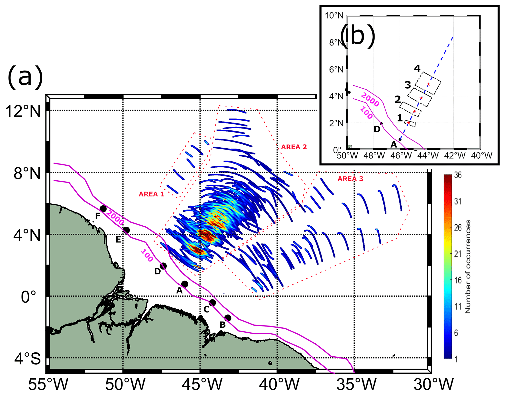
Figure 2 (a) Spatial density map of occurrences of ISW signatures visible in MODIS-Terra images. The points labeled from A to F are IT generation points, which are ordered according to their energy flux amplitudes following Tchilibou et al. (2022). (b) Location of the paths of higher occurrence of ISWs. The blue lines are the transect lines representing the IT's pathway from IT site A.

2.4 Statistical analysis

The normality of the distribution associated with each considered parameter was evaluated using the Shapiro–Wilk test (SWT). The comparison of the mean of the different groups of data considered here was then performed using a parametric test (Student t test) when the distribution of the sample was following a normal distribution, while the non-parametric test (Mann–Whitney–Wilcoxon test, MWWT) was applied when this condition was not valid or for comparison of unbalanced size groups (number of samples in one group more than 3 times the number of samples of the other one). The non-parametric Kruskal–Wallis H test (KWT) was performed to determine if there are statistical differences among more than two independent groups. The non-parametric kernel density (KD) estimation was used for probability density estimation when a parametric distribution could not properly describe our variable.

3 Results

All ISW occurrences identified off the Amazon shelf found by direct examination of images are displayed in Fig. 2. ISWs emanate from several IT generation sites along with the shelf break near the 100 m isobath as previously described by Magalhães et al. (2016) and Tchilibou et al. (2022). By analysis of the semidiurnal (M2) baroclinic flux in the region (Tchilibou et al., 2022), we divided the waves into regions (areas 1, 2, and 3) according to their likely associated IT generation sites. Area 1 may contain waves from generation sites E and/or F, and Area 2 may contain waves from sites A and D. In Area 3, ISWs likely come from sites B and/or C. A higher number of occurrences of waves is found in Area 2 compared to other areas, revealing coherent sub-patches (more than 35 occurrences) along the IT's pathway separated from each other by a typical mode-1 wavelength (see the position of the sub-patches and their middle point in Fig. 2b and the distance between the middle point of the sub-patches in Table 1), the sub-patch further northeast being structured like a tail with fine scales (sub-patch number 4). The sub-patches are organized following a similar pattern to the M2 internal-tide dissipation described by Tchilibou et al. (2022). We make the assumption that the sub-patches might correspond to the IT reflection beams at the surface or subsurface, which may generate newer ISWs when ITs become unstable (Gerkema, 2001). The distance between IT generation site A (isobath of 100 m) and the first ISW sub-patch of a higher occurrence in Area 2 is around 150 km.

The first analysis was done considering the ISWs with intra-packet distances; Fig. 3a gives further insight into the horizontal structure of the northeastward-propagating waves, revealing a largely unimodal distribution of crest lengths that are strongly skewed toward the shorter end. These ISW packets are regularly observed to reach crest lengths ranging up to 372 km, although most of the observations are characterized by crest lengths between 70 and 90 km. Unlike sun-glint-derived wave identification, SAR-derived ISWs are generally unaffected by cloud cover. This could explain the skewed distribution observed here toward lower values due to the intense cloud coverage associated with the Inter Tropical Convergence Zone near the Amazon region. The intra-packet distance distribution, which is the distance between waves of the same packet, shows a unimodal distribution shifted to the smallest distances with most of the observations ranging between 7 and 18 km, with the most frequent value being ∼ 10 km (Fig. 3b). The average intra-packet distance for the entire period is 12 km with a standard deviation of 6 km.

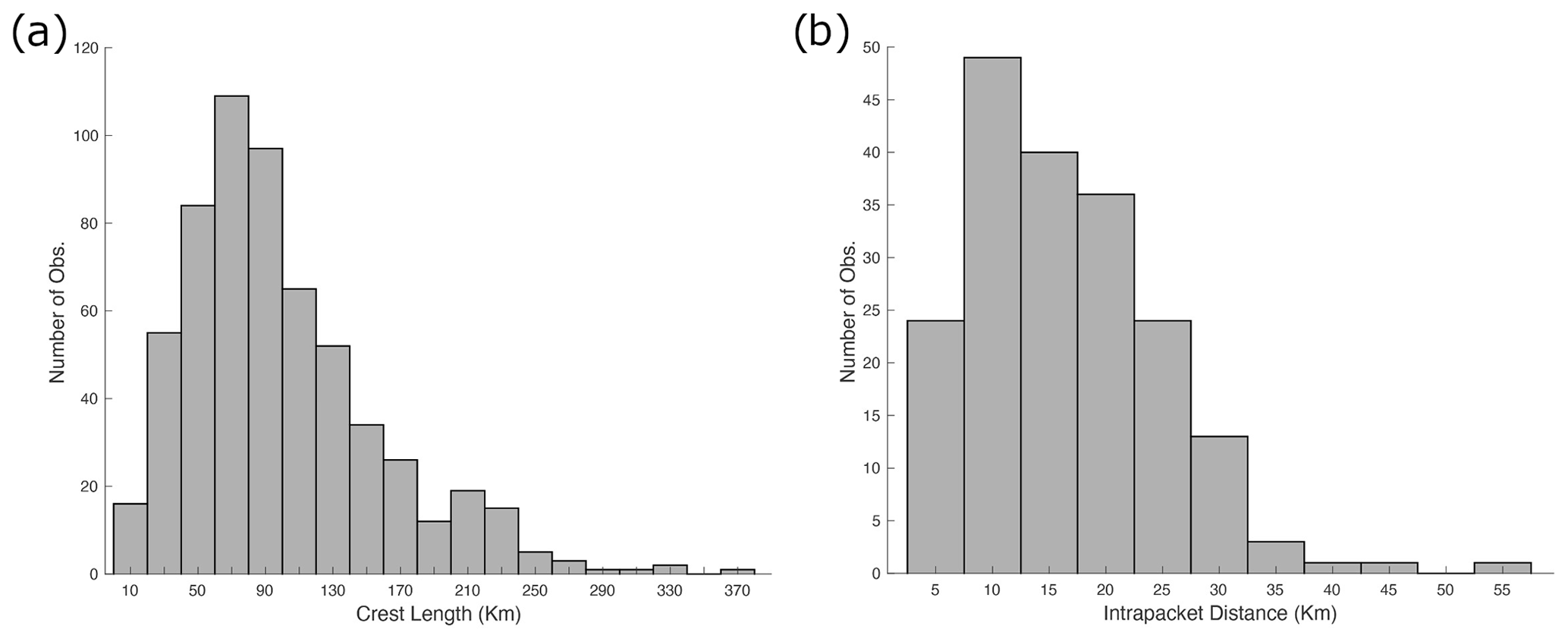
Figure 3 (a) ISW crest lengths. The average length is 99 km, with a standard deviation of 58 km. (b) ISW intra-packet distance distribution.

3.1 ISW temporal distribution of first and second baroclinic modes

The monthly and yearly number of clear images and the number of signatures per clear image (i.e., the number of identified ISW signatures according to their modes divided by the total number of images containing at least one clear signature) are presented, respectively, in Fig. 4a and b. The number of clear RS images is not equally distributed among the months, with most of the images (84 %) being identified during the dry season (less cloudy coverage) from August to October. Because of the lack of acquisitions for some months, no evident seasonal variability is found. The mode-1 waves show a more homogeneous distribution according to the years, while the number of mode-2 waves has a more evident variation. The total number of detected mode-1 waves is about 3 times the number of mode 2.

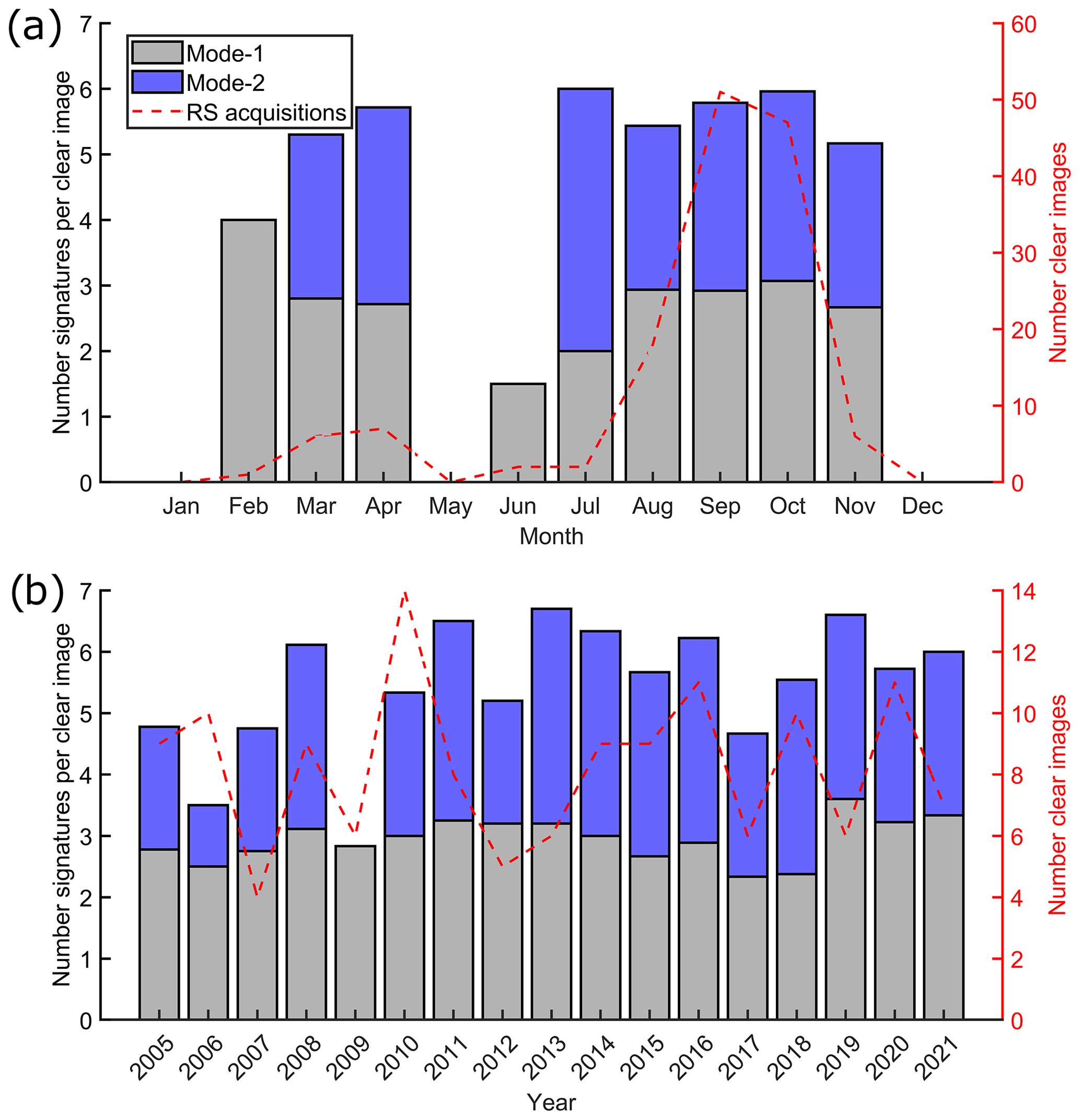
Figure 4 The monthly (a) and yearly (b) distributions of the number of RS images in which at least one ISW signature was identified (clear image; dashed red line) and the corresponding number of normalized mode-1 (gray bars) and mode-2 (blue bars) ISW signatures.

Table 1 Distance between the middle point of the sub-patches of higher occurrence of ISWs in Area 2 (red stars in Fig. 1b).

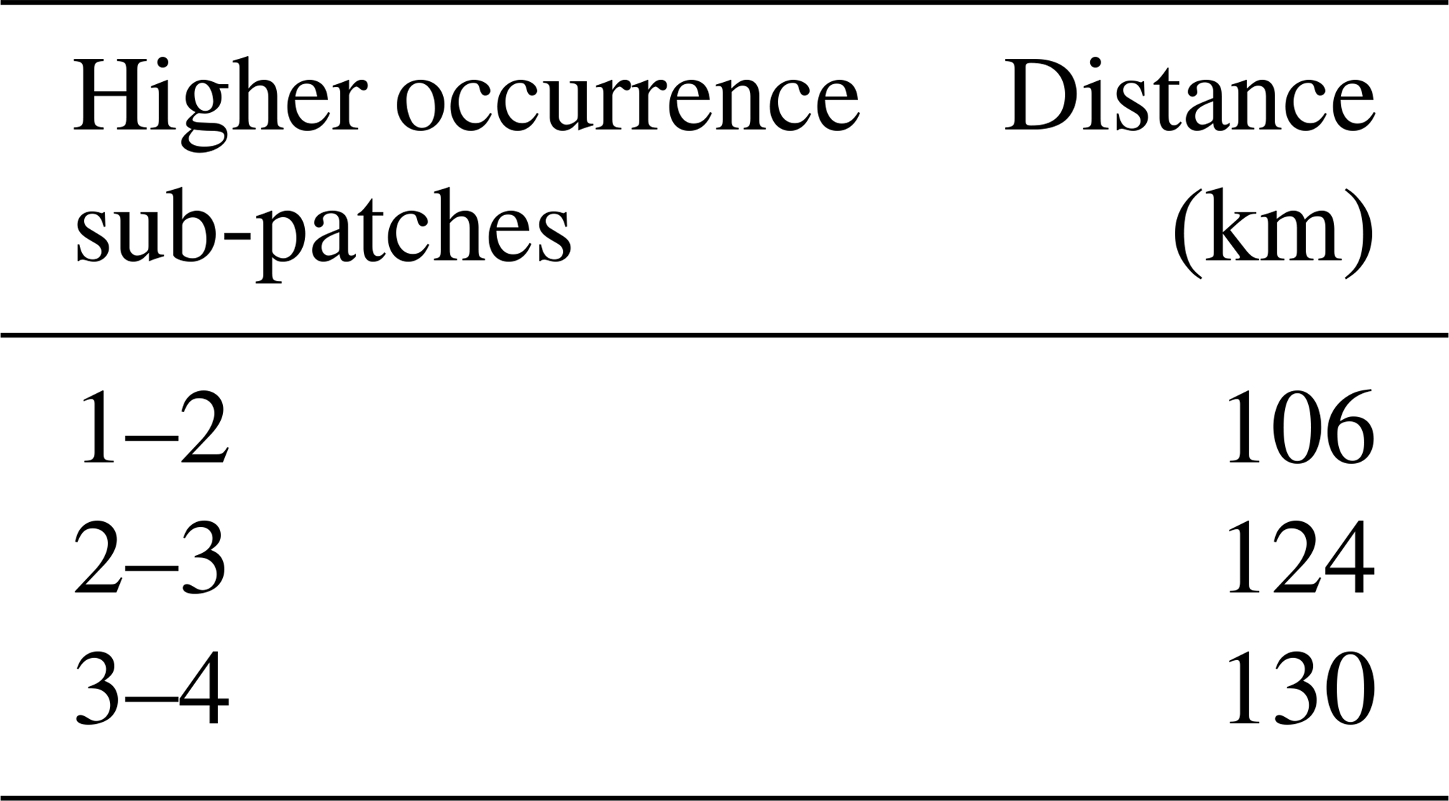
Table 2 Number of ISW signatures and values of the ISW average inter-packet distance measured from RS data and their corresponding velocity and values of IT wavelength or velocity predicted by solving the viscous TGE using monthly reanalysis data in areas 2 and 3 according to the different baroclinic modes of IT waves.

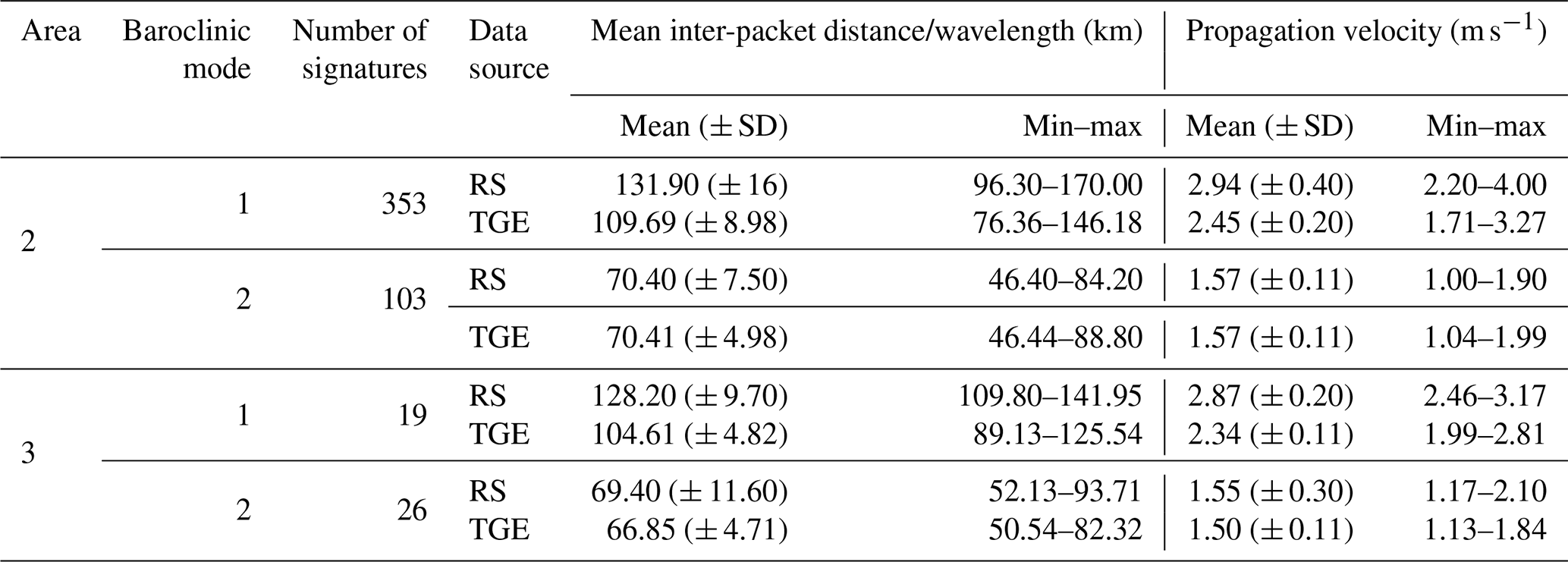
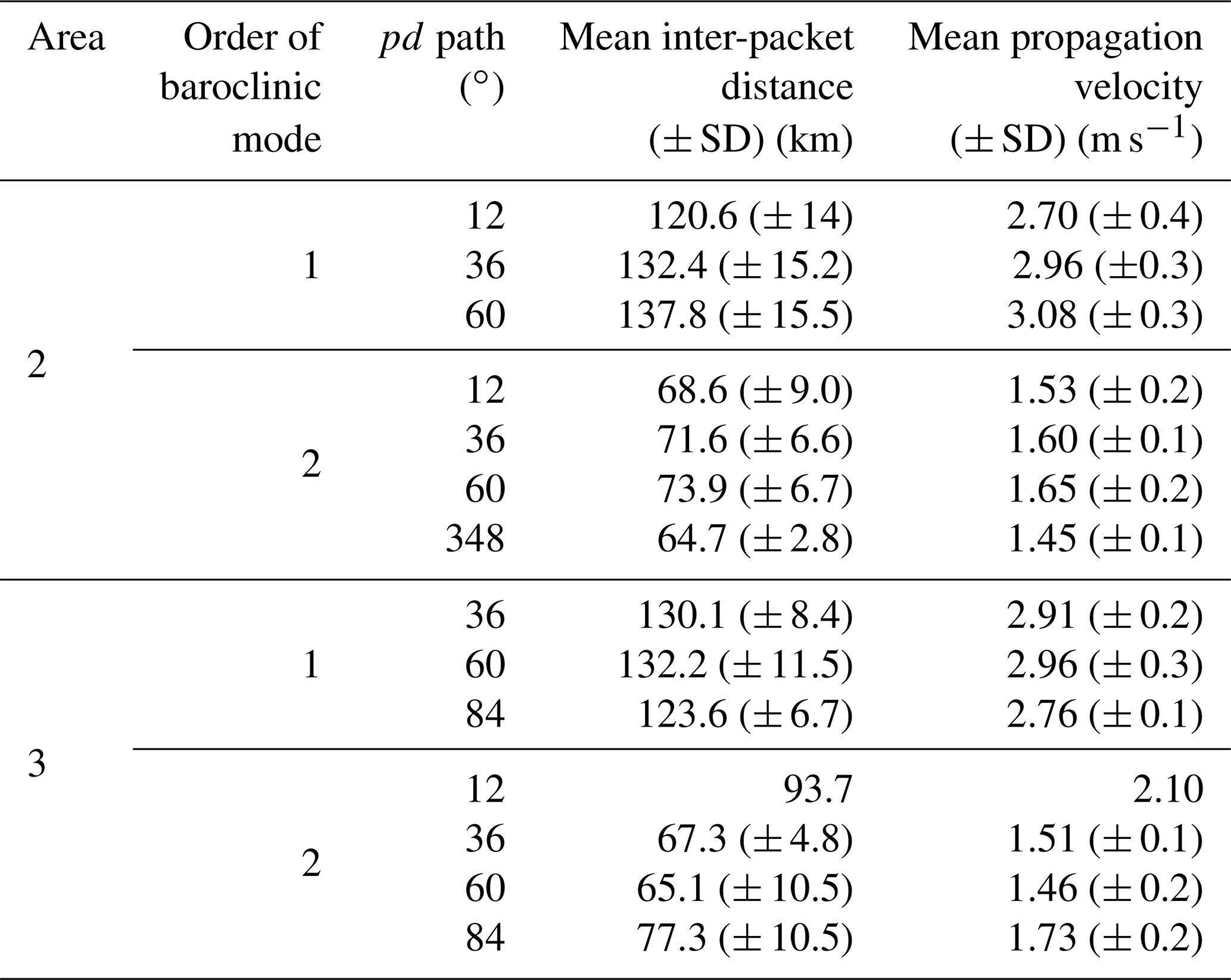
Table 3 Values of ISW average inter-packet distance measured from RS data and its corresponding velocity in areas 2 and 3 according to the different baroclinic modes of the waves and their propagation directions.

In Area 2 (waves coming from IT generation sites A and D), the wave's inter-packet distance has a bi-model normal distribution (SWT, ρ>0.5; see Fig. 5a), each group being likely associated with an ISW separated by typical mode-1 and mode-2 IT wavelengths (the group with higher inter-packet distance associated with mode-1 IT; see Table 2). The mean mode-1 and mode-2 inter-packet distances (and corresponding velocity) deduced from the RS data are, respectively, 131.90 ± 16 km (2.94 ± 0.40 m s⁻¹) and 70.40 ± 7.50 km (1.57 ± 0.20 m s⁻¹). In that area, Magalhães et al. (2016) observed ISWs of the fundamental mode propagating with similar mean velocities (i.e., 3.1 m s⁻¹). IT velocity/wavelength distribution calculated using TGE (Fig. 5b) shows a similar pattern to the RS measurements for mode-1 and mode-2 waves, supporting our decision to separate the ISWs according to the different baroclinic modes. The calculated mode-1 mean propagation velocity is underestimated by ∼ 20 %. An underestimation of the phase speed calculated by the TGE of 12 % was found in the Mascarene Plateau considering the ocean depth between 3 and 3.8 km (da Silva et al., 2011). According to Alford et al. (2010), in the South China Sea, nonlinear waves of M2 frequency travel at a phase speed 1.5 times the linear wave phase speed. The nonlinear phase speed can be corrected using the Korteweg–de Vries (KdV) equation (Hammack and Segur, 1974; Alford et al., 2010); however, this theory applies only to shallow waters with uniform depths, which is not the case in our study area. The KdV equation would increase the mean wave speed by about 16 % for mode-1 waves, considering a maximum wave elevation of 100 m Brandt et al. (2002).

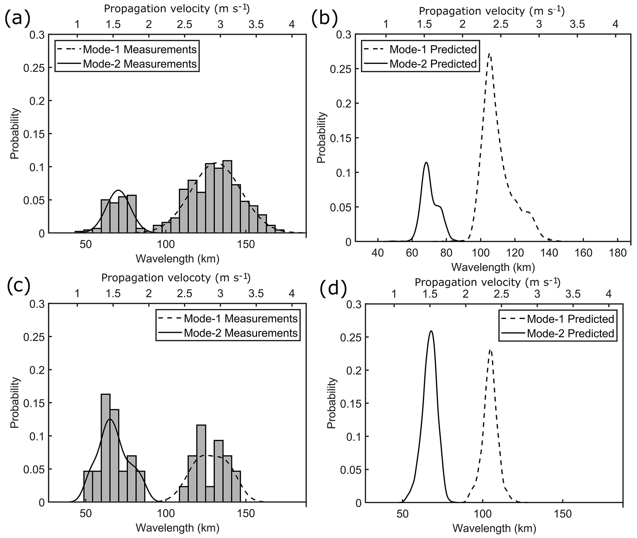
Figure 5 Histogram of ISW inter-packet distance for (a) Area 2 and (c) Area 3 in gray color. The fitted normal distribution of the ISW inter-packet distance calculated from the RS data is shown as black lines. KD of the predicted velocities/wavelength by solving the TGE using monthly reanalysis data for (b) Area 2 and (d) Area 3. Mode-1 and mode-2 waves are shown as dotted and continuous lines, respectively.

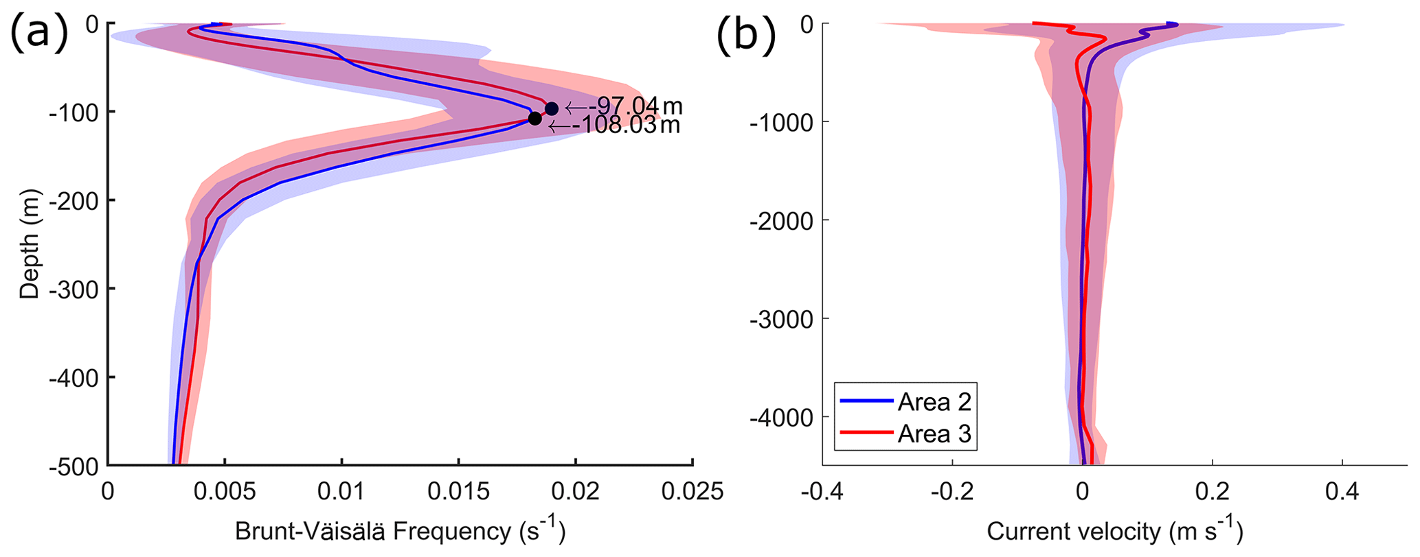
Figure 6 (a) Brunt–Väisälä frequency and (b) mean current velocity decomposed along the ISW traveling direction for areas 2 and 3 derived from the EPR data. The bands represent the standard deviation over the period from 2005 to 2019.

In Area 3 (waves coming from IT generation sites B and/or C), in contrast with Area 2, the number of mode-2 signatures is higher than mode 1 by 1.3 times (see Table 2). The depth of the pycnocline in the study area was defined as the depth corresponding to the maximal value of the Brunt–Väisälä frequency. A slightly shallower pycnocline with higher maximum values of the Brunt–Väisälä frequency is found in Area 3 compared to Area 2 (see Fig. 6a), suggesting that stronger higher-mode internal-tide generation is expected (Barbot et al., 2021; Tchilibou et al., 2022) in good agreement with our findings. The ISW inter-packet distance distribution has a bi-modal normal distribution similar to Area 2 (Fig. 5c). The mean mode-1 and mode-2 inter-packet distances (and corresponding velocity) deduced from the RS data are, respectively, 128.20 ± 9.70 km (2.87 ± 0.20 m s⁻¹) and 69.40 ± 11.60 km (1.55 ± 0.30 m s⁻¹). For the ISW of the fundamental mode, Magalhães et al. (2016) found waves with a similar mean propagation velocity in Area 3 (i.e., 2.7 m s⁻¹). The TGE allows a relevant prediction of the IT propagation velocity/wavelength distribution of mode-1 and mode-2 waves, with mode-1 velocities being underestimated by 22 % and mode 2 by 3.7 % (Fig.  5d). The mode-1 and mode-2 mean propagation velocity/wavelength values do not vary significantly according to the different study areas (ρ>0.5, MWWT).

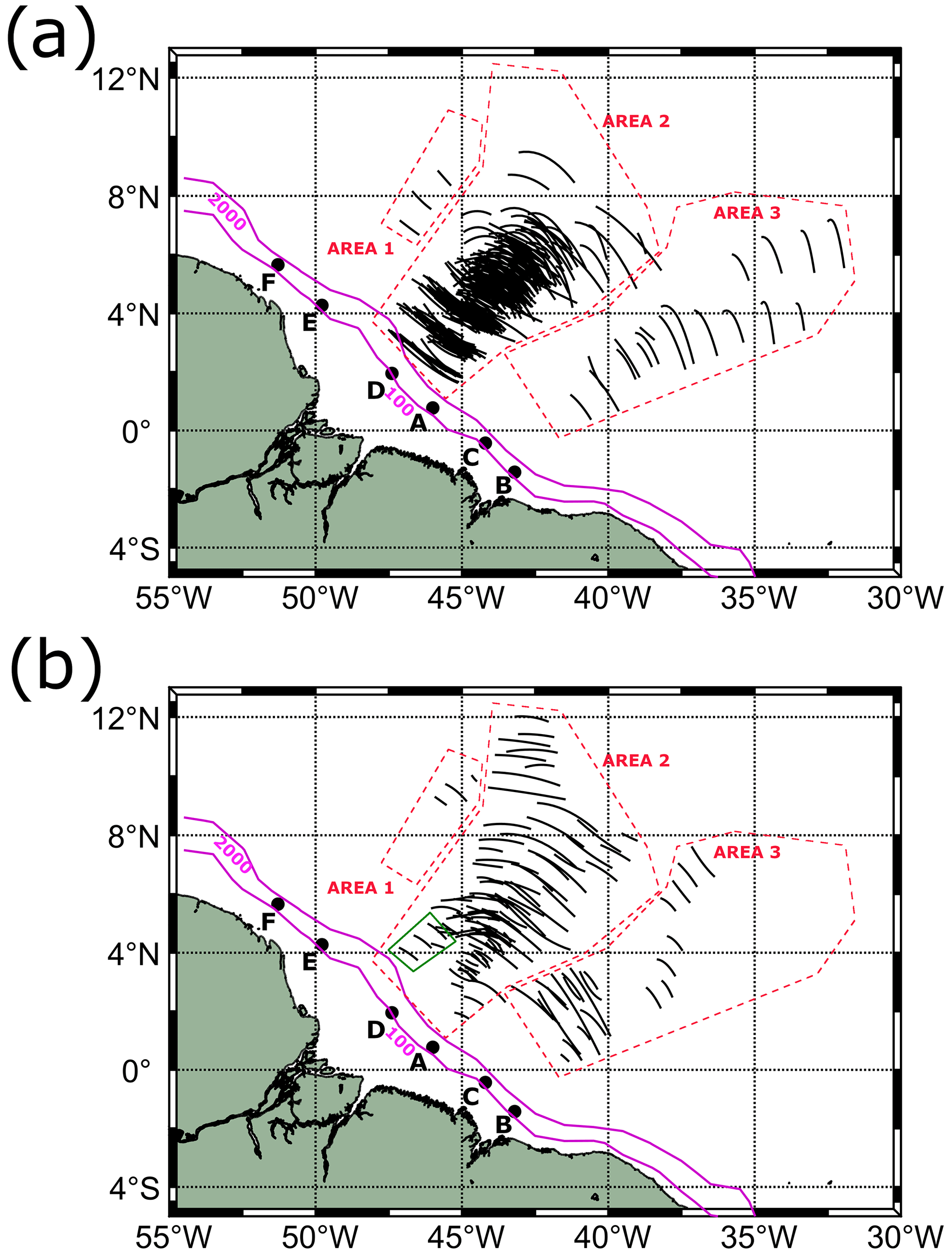
Figure 7 (a) Mode-1 and (b) mode-2 ISW composite map derived from 140 MODIS-Terra data acquired under sun glint conditions from 2005–2021. All identified signatures were considered and depicted on the map, with a total of 507 signatures, of which 375 are associated with mode 1 and 132 correspond to mode-2 internal waves.

Looking now at their horizontal distribution, mode by mode (Fig. 7), the analysis of the mode-2 signatures clearly shows wave signatures emanating from the D site and joining Area 2 (see the green rectangle in Fig. 7b). This example of joining rays of propagation may explain why this region is the strongest as it focuses rays from D as well. Considering the small number of signatures that come from Area 1, the analysis presented in our paper does not consider those signatures. However, combining other satellite sensors might help retrieve a stronger signal from this site (Rosa et al., 2021).

The spatial distribution of the mode-1 and mode-2 waves according to their propagation velocities (respectively, Fig. 8a, b) allows discriminating between two main branches of waves propagating in different directions in Area 2, where the most eastern branch is associated with higher propagation speed. Globally a higher contrast is found for the branches of the mode-2 waves in terms of both velocities and spatial location when compared to mode 1. In Area 2, an offshore acceleration is also further observed for the most eastern branch of both mode-1 and mode-2 waves (see Fig. 8c and d, where a cross-shore profile was done and the corresponding values of propagation velocity along the profile were retrieved). The acceleration is slightly more pronounced for mode-2 waves with an offshore increment in the propagation velocities of ∼ 18 %, while the increment for the mode-1 waves is ∼ 15 %.

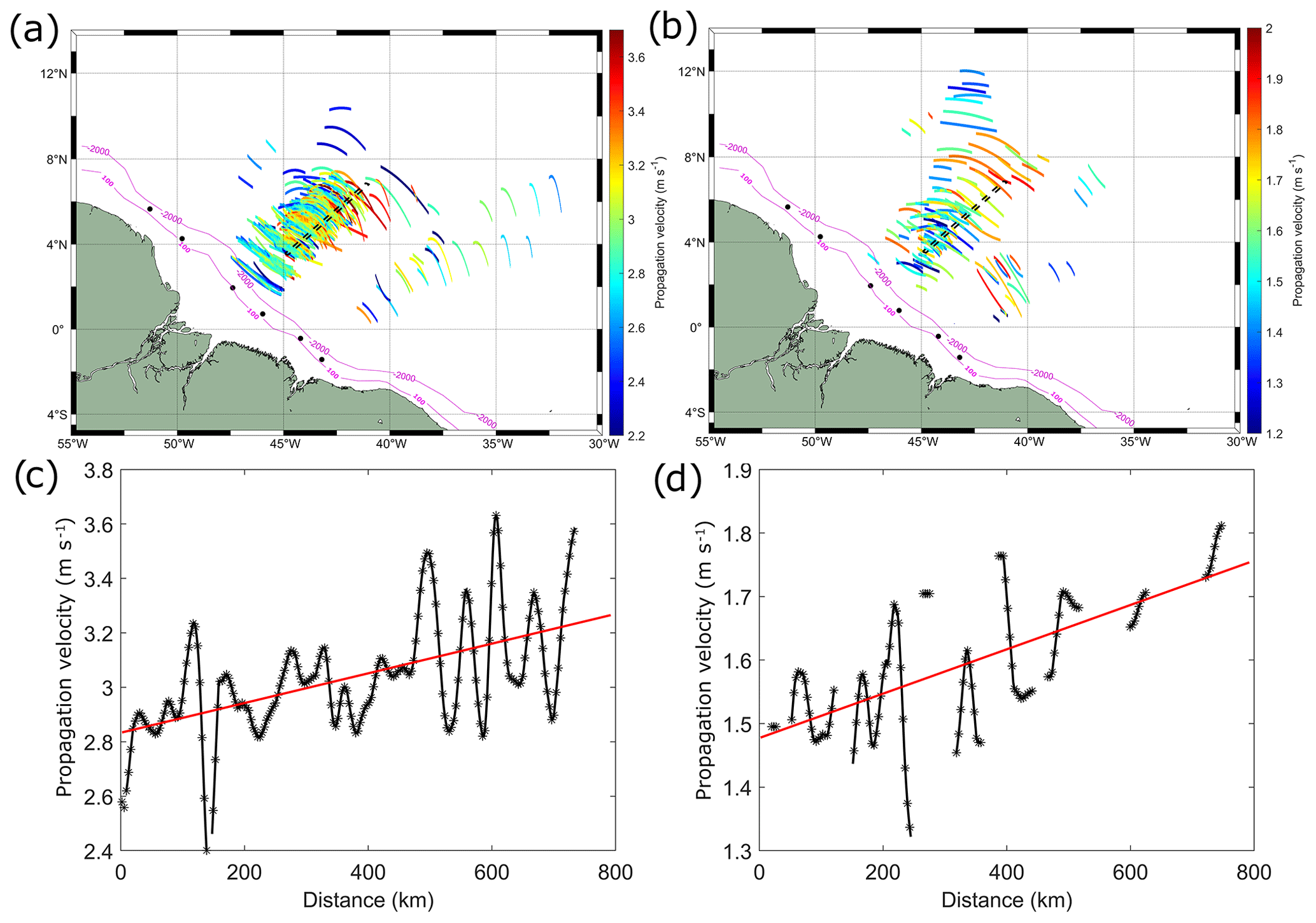
Figure 8 Propagation velocities of the (a) mode-1 and (b) mode-2 internal waves off the Amazon shelf. The dashed black rectangle represents the selected cross-shore profile. Cross-shore profile of the ISW propagation velocities for (c) mode-1 and (d) mode-2 waves derived from the RS data. The red line is the fitted linear regression model for the measurements.

The characterization of the propagation direction of the ISWs (Fig. 9) shows us that, in Area 2, mode-2 waves propagate in a wider range of directions compared to mode-1 ones. The mean inter-packet distance and corresponding velocity tend to increase with the increase in the eastern traveling direction component (for both mode 1 and mode 2, there are significant differences between the ISW propagation direction paths; i.e., ρ<0.01, KWT; Table 3; the paths with a probability lower than 0.2 were excluded from the analysis). This increasing pattern is even more pronounced for the mode-2 waves than for mode 1 (respectively, an increase of 4 % and 7.8 %). This suggests that when deviated to the east, the waves are accelerated by regional eastward currents.

In Area 3, for both mode 1 and mode 2, waves for the different propagation paths do not differ statistically in terms of their inter-packet distance/velocity (ρ>0.5, MWWT and t test). Area 3 is less influenced by the NECC than Area 2. As a matter of fact, current velocities decomposed on the ISW traveling direction are less than half of the respective values found in Area 2, with a higher negative component (i.e., the current flowing in the opposite direction to the waves' traveling direction; Fig. 6b). Compared with the mode-1 waves, the mode-2 ones have a stronger northern component and propagate in a wider pathway in both areas. In Area 3, mode-1 and mode-2 waves travel in a more eastward direction.

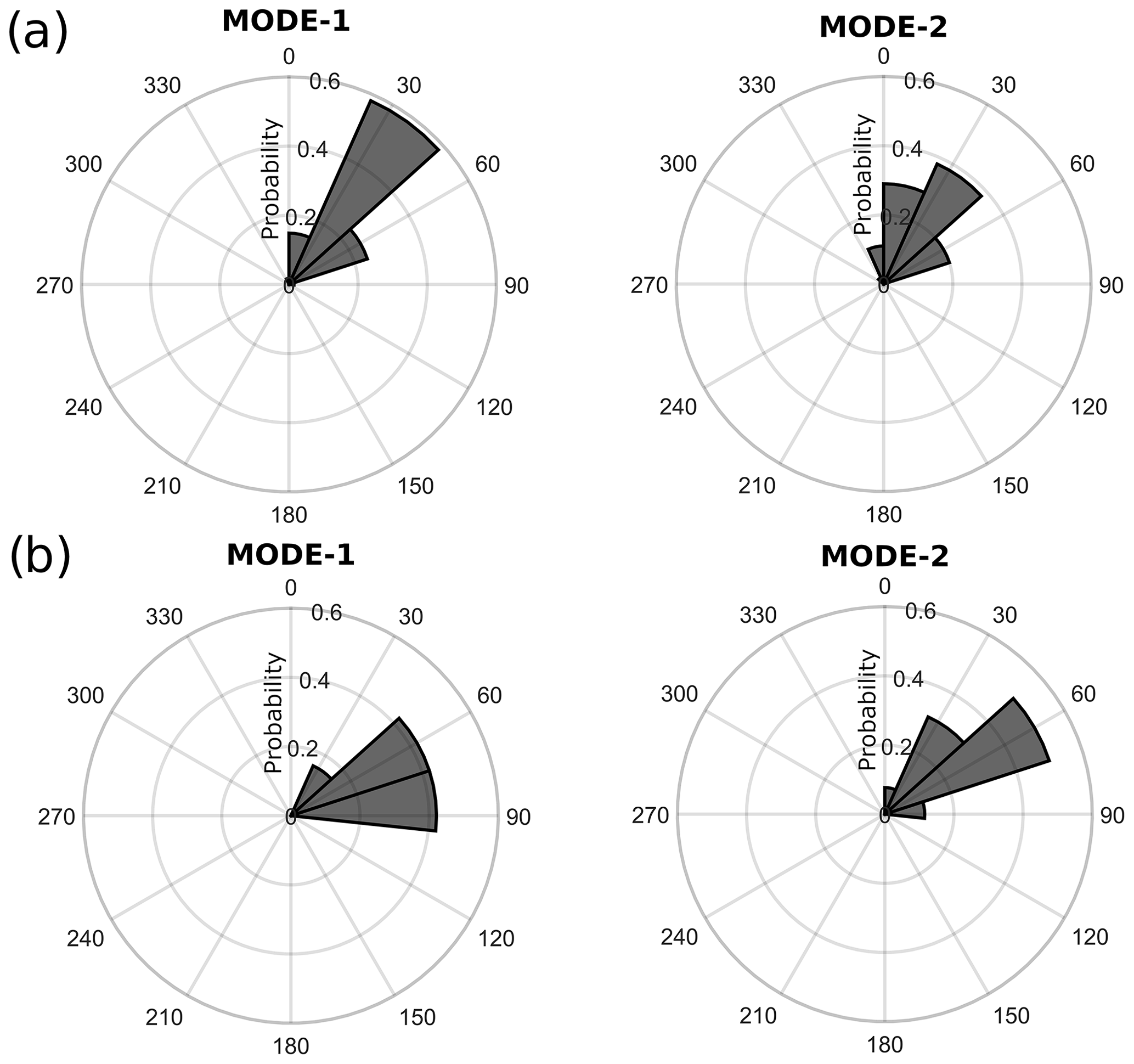
Figure 9 ISW propagation directions for (a) Area 2 and (b) Area 3. ISW propagation angles are given clockwise from the north. A $pd=\mathrm{0}{}^{\circ }$ denotes ISWs propagating from the south to the north, and $pd=\mathrm{90}{}^{\circ }$ denotes ISWs from the west to the east.

3.1.1 Spring–neap tidal variability

The occurrence of ISWs according to the tidal conditions (i.e., near-neap and spring tides) has been investigated for both areas 2 and 3. Near-spring tide is defined as ± 3 d after spring tide peak. A more detailed description of wave propagation velocities and direction variability according to the spring–neap cycle was performed in Area 2 but not in Area 3 because of the lack of measurements in that area.

Analysis of the RS data revealed that the ISW activity is more pronounced in near-spring tide conditions for both areas (71 % of the ISW signatures for Area 2 and 61 % for Area 3). This result is in line with previous studies where higher wave activity in near-spring tide has been reported (New and da Silva, 2002; da Silva et al., 2011; Liu and D’Sa, 2019) compared to near-neap tide. In both areas, there are more mode-2 waves during neap tides than spring tides (near-neap and spring tide, in Area 2, respectively, 28 % and 20 % and, in Area 3, 61 % and 48 %).

For Area 2, the mode-1 mean inter-packet distance varies according to the different tidal conditions (p<0.01, t test; Fig. 10a). Higher inter-packet distances are associated with the wave signatures found in near-neap tide (137.6 ± 15.2 km and 3.1 ± 0.3 m s⁻¹); in contrast, in near-spring tide, the mean ISW inter-packet distance decreases by about 6 % (129.8 ± 16.1 km and 2.9 ± 0.4 m s⁻¹), implying a corresponding decrease in the propagation speed. This analysis may be hampered by our unbalanced data set, as stronger tides would suggest larger ITs being generated with higher propagation velocities. For the mode-2 waves, no significant differences are found according to the tide conditions (p>0.05, t test); see Fig. 10b. The mean inter-packet distances for near-spring and neap tides are, respectively, 70.16 ± 7.59 km (1.57 ± 0.17 m s⁻¹) and 70.67 ± 7.55 km (1.58 ± 0.17 m s⁻¹). No significant differences are found in the propagation direction according to the spring–neap tides, for both mode-1 and mode-2 waves (figure not shown).

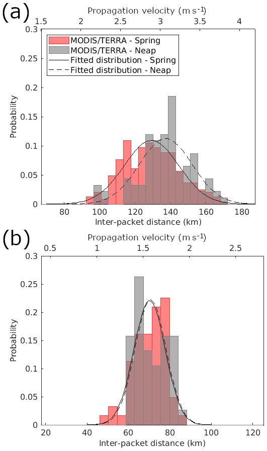
Figure 10 Fitted Gaussian distribution of the (a) mode-1 and (b) mode-2 ISW inter-packet distance and corresponding propagation velocity according to the neap (dotted line) and spring (continuous line) tides.

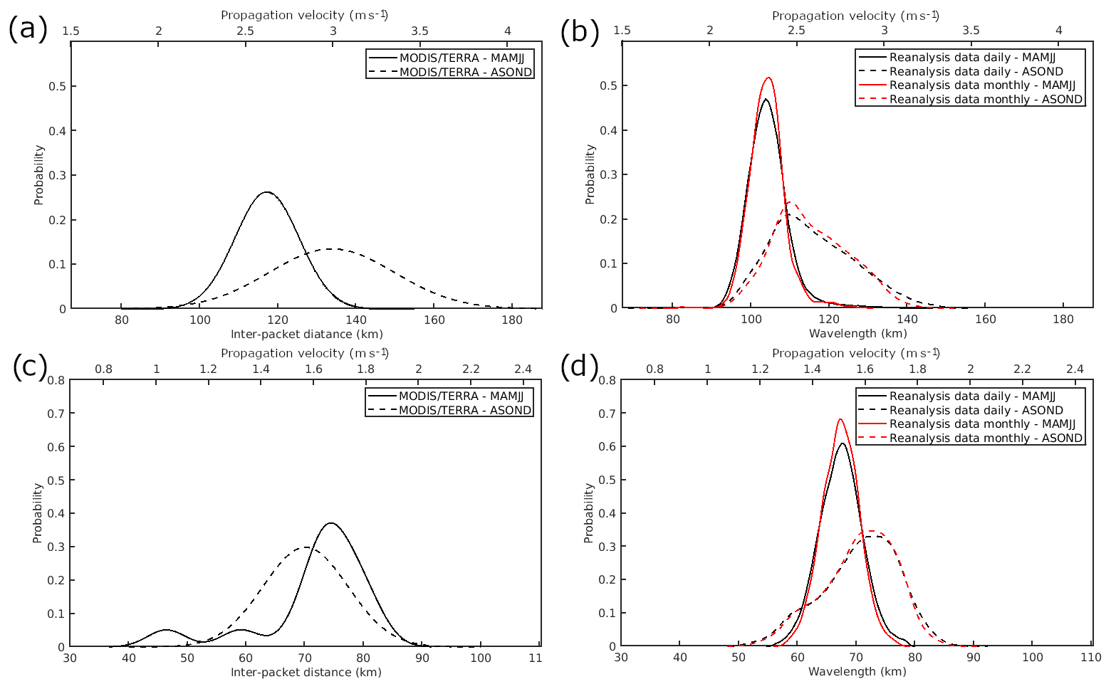
Figure 11 Fitted distribution of the ISW inter-packet distance and corresponding propagation velocity measured from the RS data for (a) mode-1 and (c) mode-2 waves for Area 2. Fitted distribution of the IT's propagation velocity/wavelength predicted by solving the TGE using daily and monthly reanalysis data: respectively, black and red lines for (b) mode-1 and (d) mode-2 waves. MAMJJ and ASOND are shown, respectively, as continuous and dashed lines.

3.1.2 Seasonal variability

The seasonal variability in the ISW in terms of its inter-packet distance and propagation direction has been further characterized considering the two well-marked seasons on the Amazon shelf, i.e., MAMJJ and ASOND following Tchilibou et al. (2022). We only apply this analysis to the waves in Area 2 because of the lack of measurements during MAMJJ in Area 3. The mode-1 waves have a 14.3 % higher mean inter-packet distance during ASOND (p<0.01, MWWT; see Fig. 11a and Table 4) than during MAMJJ, implying a corresponding increase in the propagation speed. The pycnocline during ASOND is slightly deeper when compared to MAMJJ (by 11 m; see Fig. 12a). Larger wavelengths (higher velocities) of mode-1 ITs are expected during ASOND compared to MAMJJ following previous studies (Liu and D’Sa, 2019; Barbot et al., 2021; Tchilibou et al., 2022). Furthermore, the mean current velocity decomposed on the ISW traveling direction has a stronger positive component during ASOND when compared to MAMJJ (Fig. 12b). Hence circulation and stratification probably act constructively to increase the IT wavelength during ASOND, in contrast to MAMJJ. During ASOND, the ISWs are characterized by a higher diversity in terms of their inter-packet distance (higher standard deviation) when compared to MAMJJ, suggesting a higher variability in the local stratification and current shear patterns in the study area during this season. Note that our samples are unbalanced according to the season, i.e., during ASOND, we have about 8 times more samples than for MAMJJ.

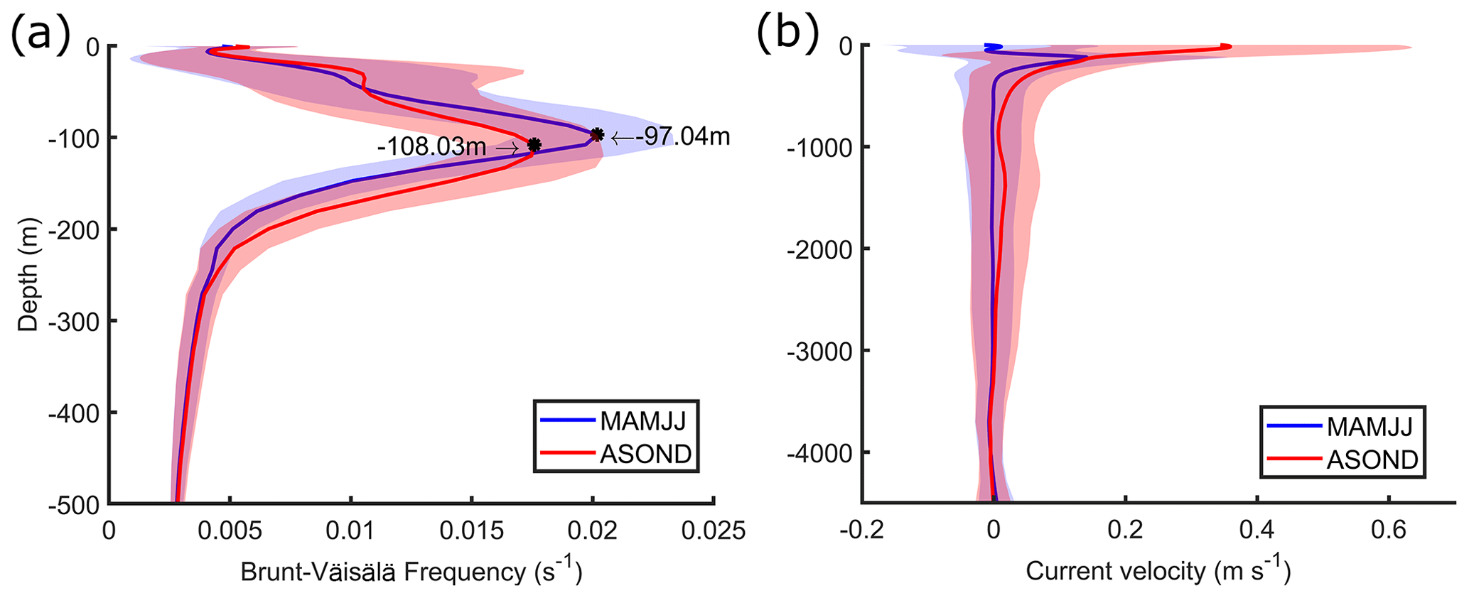
Figure 12 (a) Brunt–Väisälä frequency and (b) mean current velocity decomposed along the ISW traveling direction in Area 2 for MAMJJ and ASOND derived from the EPR data. The bands represent the standard deviation over the period from 2005 to 2019.

Table 4 Values of ISW average inter-packet distance measured from RS data and its corresponding velocity and values of IT wavelength/velocity predicted by solving the viscous TGE using daily and monthly reanalysis data in Area 2 according to the seasons and the different baroclinic modes of the waves.

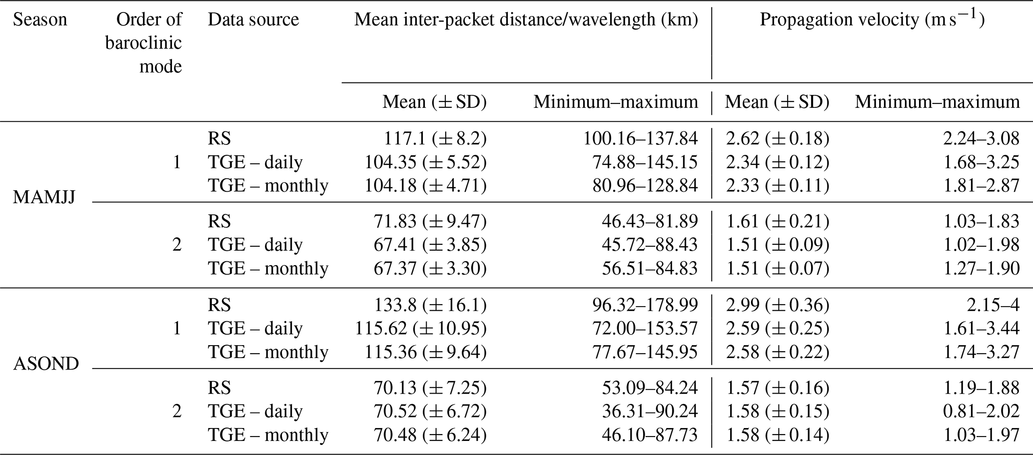
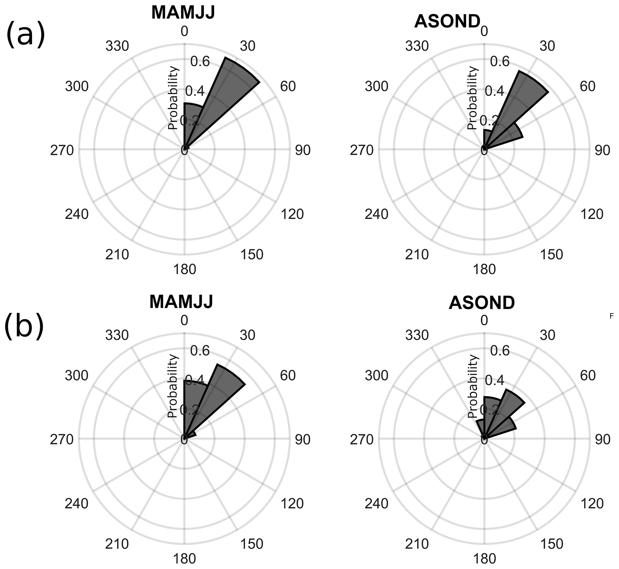
Figure 13 ISW propagation directions for (a) mode-1 and (b) mode-2 waves in Area 2 according to the season. ISW propagation angles are given clockwise from the north. A $pd=\mathrm{0}{}^{\circ }$ denotes ISWs propagating from the south to the north, and $pd=\mathrm{90}{}^{\circ }$ denotes ISWs from the west to the east.

The TGE is able to predict the differences in the mode-1 IT velocities/wavelengths between the two seasons (p<0.01, MWWT) with a distribution pattern similar to the one estimated using the RS data (see Fig. 11b). However, the differences between the two seasons are less evident considering the values predicted by the TGE (mean wavelength value increases by 9.5 % during ASOND when compared to MAMJJ). Compared to the RS data, the mean waves' wavelengths are underestimated by 11 % and 14 %, respectively, for MAMJJ and ASOND (Table 4). The mean velocity/wavelength values predicted using daily and monthly reanalysis data are very similar for both seasons. Differences in their standard deviation (standard deviation slightly higher for daily reanalysis data compared to the monthly ones) indicate that using monthly data probably tends to smooth the variability related to stratification and circulation.

The mode-2 ISW inter-packet distance and corresponding propagation velocity do not vary according to the different seasons (p>0.05, MWWT); see Fig. 11c and Table 4. In contrast, the mean mode-2 IT propagation velocities/wavelength calculated by the TGE is 4.6 % higher during ASOND than MAMJJ, and, during ASOND, the distribution of the predicted velocities fits the RS data quite well. The TGE seems to underestimate the wave propagation velocities by 6.5 % during MAMJJ. It is important to point out that the mode-2 signatures identified from the RS observation are not well balanced between the seasons and the period of MAMJJ counts with only 13 samples, probably impairing our analysis.

During ASOND, the mode-1 and mode-2 ISWs propagate in a wider direction pathway (Fig. 13). The increase in the mode-1 and mode-2 ISW inter-packet distances with an increasing eastern traveling direction component shown before (see Sect. 3.1) is found only during ASOND (no differences in the inter-packet distances of the waves are found during MAMJJ; p>0.05; Mann–Whitney U nonparametric test). In the months of ASOND, the circulation is characterized by the eastward reinforcement of the NECC, which likely plays a role in refracting the waves to the east (as also pointed out by Magalhães et al., 2016) and in increasing their propagation velocities eastward. Furthermore, as a consequence of the more dynamic mesoscale circulation associated with ASOND, the ISWs seem to spread over the study area during this season (Fig. 14), extending the wave penetration further north principally at the end of the boreal summer and early fall (August–October) when maximum values of eddy vorticity are found (Aguedjou et al., 2019). This behavior contrasts with the more straightforward path and lower penetration further north associated with the waves in the months of MAMJJ. Most of the ISW signatures in Area 2 above the latitude 8^∘ N correspond to mode-2 waves from early September 2014 and 2018. However, it is important to point out that this can result from sampling restrictions due to the combination of higher cloudy coverage and the location of the sun glint area during the months of MAMJJ.

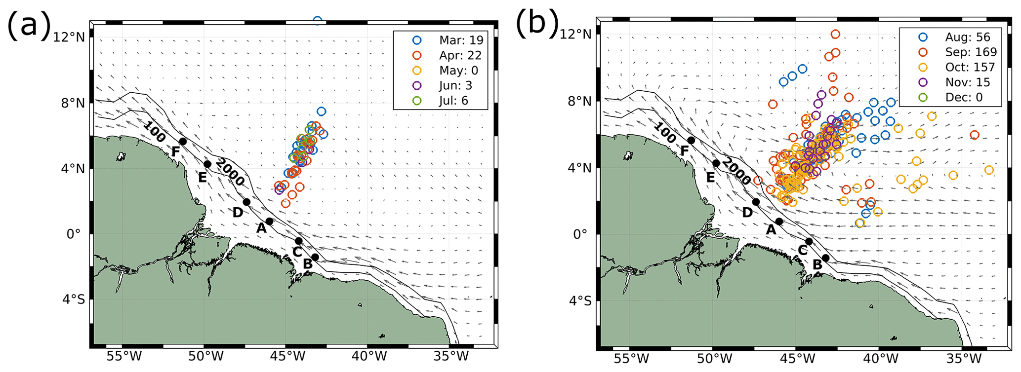
Figure 14 Location of the ISW signatures associated with mode-1 and mode-2 internal tides for (a) MAMJJ and (b) ASOND. The colors represent the months when the signatures were identified. The points represent the middle point of each wave signature, and the arrows depict the mean surface current speed and direction for each season derived from the EPR data. The number of ISW signatures occurring per month can be found in the legend.

The time–space variability in the IT's phase velocity associated with changes in the background current and stratification is exploited as a proxy for the variability in the waves' propagation direction (refraction). Maps of the seasonal coefficient of variation in the mode-1 and mode-2 IT phase velocities calculated by the TGE using the monthly average EPR data are shown in Fig. 15. Changes in the phase velocity are more evident for mode-2 waves than mode-1 ones in both seasons, in good agreement with our results, which show mode-2 waves as probably more sensitive to changes in the circulation patterns in the study area. In Area 2 (waves coming from IT generation point A and D), the variability in the phase velocity is higher during ASOND than during MAMJJ. Furthermore, during ASOND the variability is aligned with the core of the NECC, in good agreement with our results. In Area 3, a different pattern occurs since higher variability is found during MAMJJ than ASOND. However, further analysis in that area is compromised because of the lack of measurements.

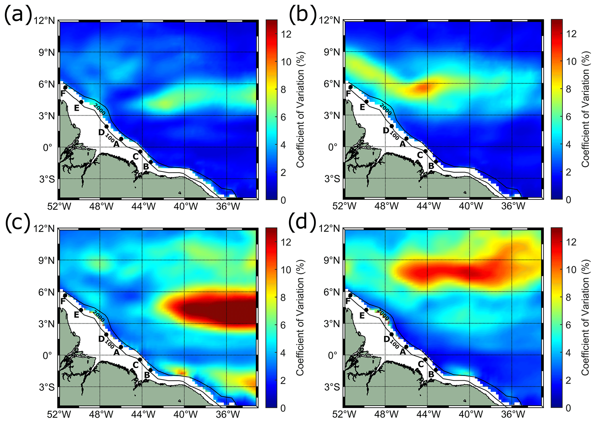
Figure 15 Maps of the seasonal coefficient of variation in the (a, b) mode-1 and (c, d) mode-2 IT phase velocities calculated by the TGE using monthly average EPR data for (a, c) MAMJJ and (b, d) ASOND.

4 Summary and discussion

This study focuses on the Amazon ISW occurrence and parameters, such as position, direction of propagation, wave inter-packet distance and its corresponding velocity, and variability at seasonal and spring–neap tidal cycles. The analysis is based on a data set of 140 MODIS-Terra images, where about 500 ISW signatures were identified in the sun glint area.

Area 2 has been pointed out in our analysis as the one with stronger ISW activity containing about 450 signatures, likely because it focuses rays emanating from both sites A and D. The region where the waves from A and D join the same path corresponds to the third patch of occurrence from the shelf break, with higher occurrences of ISWs (see Fig. 2). Tchilibou et al. (2022) found IT generation sites A and B with quite similar M2 baroclinic flux horizontal divergence, but with site A being more efficient in converting the flux into ITs. In Area 2, the distance between generation point A (isobath of 100 m) and the first patch of high occurrence is around 150 km. Regions of higher occurrence of ISWs are structured into sub-patches separated from each other by a mode-1 typical wavelength (see Table 1), and we suppose the regions might correspond to the IT reflection beams at the surface. Gerkema (2001) discussed the local wave activity in the thermocline in the Bay of Biscay due to the scattering of the internal-tide beam, which scatters strongly at a moderately developed thermocline. The patch further northeast (number 4 in Fig. 2b) is structured as a tail with finer scales, being noisier as the wave gets unstable to higher modes. The waves propagate about 350 km without dissipation and then suffer changes in their wavelength, which could indicate some instability, a transfer to higher modes, or dissipation. Our finds are fit in with the results presented in Tchilibou et al. (2022).

Previous studies have documented the existence of mode-1 ISW (Magalhães et al., 2016), but in fact, the region appears as a newly described hotspot for small-scale ISWs with an average inter-packet distance with a typical wavelength of mode-2 ITs. The coexistence of mode-2 solitary-like waves and mode-1 ISW has been documented in the literature, for example, on the Mascarene Ridge (da Silva et al., 2015) and in the Andaman Sea (Magalhães and da Silva, 2018; Magalhaes et al., 2020). The ISW inter-packet distance deduced from the RS data showed a bi-modal distribution with two well-separated peaks for both areas 2 and 3, allowing us to separate the ISW associated with two IT baroclinic modes: a wavelength (velocity) ranging from 95–170 km (2.1–3.8 m s⁻¹) for mode 1 and a wavelength ranging from 46–85 km (1.0–1.9 m s⁻¹) for mode 2. Using results from ocean modeling, Barbot et al. (2021) found IT horizontal surface wavelengths varying from 110–120 and 70–80 km for mode-1 and mode-2 ITs in that study area. This result is in fair agreement with our results considering that nonlinear effects associated with the ISWs increase the phase speed of the waves and the variability in current and stratification that explain our more dispersive results compared to the model. In contrast, Assene et al. (2023) found wavelengths varying from 140–160 km. Zhang and Li (2022), using a data-driven machine learning model, found a bi-modal distribution of the ISW phase speed in the region, with a wide range of velocities from values lower than 1 m s⁻¹ up to 4 m s⁻¹. Although the underestimation of the mode-1 wavelengths/velocities by the TGE in the study area is of the order of 20 %–22 %, the simulated wavelengths/velocities showed two well-separated distributions for mode-1 and mode-2 waves with a similar pattern to the one deduced from the RS data supporting our decision to split the waves according to their different baroclinic modes.

The range and values of ISW with typical mode-1 and mode-2 IT wavelengths do not show significant differences according to areas 2 and 3. However, Area 3 seems to have a higher proportion of mode-2 by mode-1 waves when compared to Area 2 (i.e., stronger higher-mode internal-tide generation) likely linked to its shallower pycnocline with higher maximum values when compared to Area 2 (see Fig. 6). However, we cannot rule out the fact that ISWs emanating from IT generation site C may be influencing these results since according to Tchilibou et al. (2022) site C is the most favorable to local dissipation (higher-mode generation connected to a higher probability of instability, thus higher local dissipation). In both areas, neap–spring tidal variability is found; i.e., the wave activity is higher during near-spring tides than near-neap tides, which is coherent with the larger tidal currents during this cycle. This result is in line with former studies where higher wave activity in near-spring tide conditions has been also pointed out (da Silva et al., 2011; Liu and D’Sa, 2019). In addition, the proportion of mode-2 by mode-1 waves seems to increase from spring to neap tide conditions.

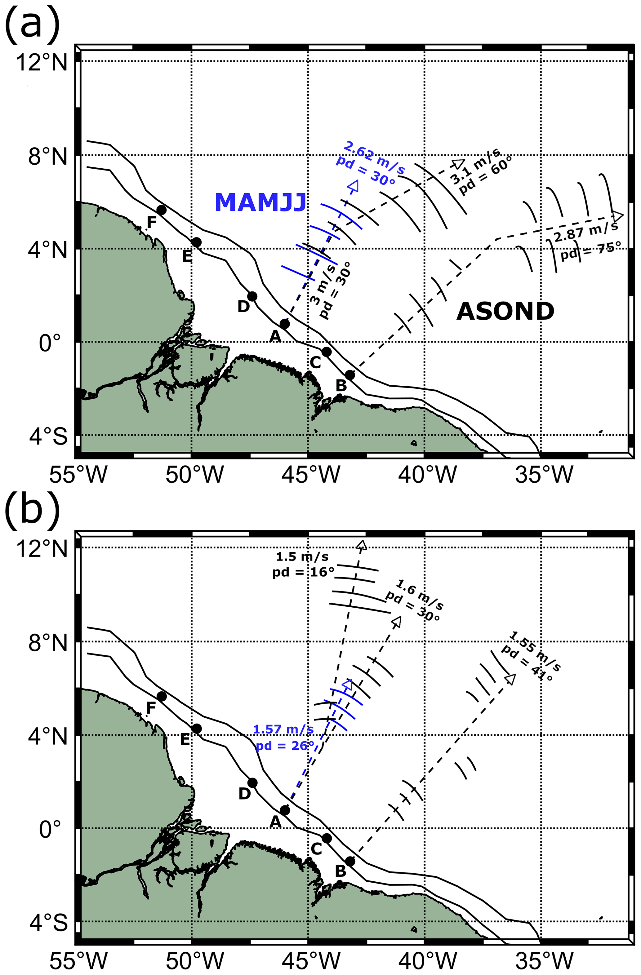
Figure 16 Synthesis of the (a) mode-1 and (b) mode-2 ISW propagation direction and velocity according to the different seasons.

Seasonal variability in the mode-1 ISWs was found in Area 2, where a higher diversity (higher standard deviation) and higher values of inter-packet distance and corresponding velocity were noticed during ASOND in contrast to MAMJJ (mean inter-packet distance/velocity 14.3 % higher during ASOND). The joint effect of higher values of mean background current velocities along the ISW traveling direction and a deeper but less stratified pycnocline (smaller Brunt–Väisälä frequency; see Fig. 12) may explain the increase in these parameters during ASOND in agreement with Barbot et al. (2021) and Tchilibou et al. (2022). Barbot et al. (2021) found that a deeper pycnocline due to large anticyclonic eddies of the North Brazil Current (NBC) mostly from August to November increases the horizontal surface wavelengths of both mode-1 and mode-2 ITs with a stronger impact on mode 1. No seasonal changes in the mode-2 ISWs inter-packet distance are found in contrast to the mode-1 one. However, it is important to point out that the limited number of mode-2 ISW samples in Area 2 during MAMJJ likely impaired our analysis. Using the TGE, the seasonal variability in predicted mode-1 and mode-2 ITs was examined. Although the differences in the mode-1 propagation velocities/wavelength between ASOND and MAMJJ are underestimated by the theoretical method, TGE could reproduce the seasonal differences in the IT wavelength giving us confidence in our previous results and supporting our analysis, principally considering our unbalanced data set according to the seasons. Furthermore, the TGE could reproduce the higher diversity of IT wavelengths during the period of ASOND than during MAMJJ, in agreement with our satellite measurements.

Finally, the comprehensive data set constructed during our analysis will support further studies to assess the impact of ISWs on the biological and biogeochemical dynamics in the study area with an emphasis on their impact on the phytoplankton biomass spatial–temporal variability.

4.1 Impact of NBC

In the region of the NECC, the direction of propagation for all modes is very similar in MAMJJ (about 30^∘ from the north), whereas, for ASOND, the ISWs propagate in a wider pathway (from 0 to 60^∘ from the north), due to a much larger eddy activity. The circulation can likely be identified as one important factor in the change in the velocities of the waves according to the different propagation direction paths. The eastward reinforcement of the NECC during ASOND seems to play a role in refracting the waves more eastward in Area 2, increasing their velocities with an increasing east-traveling direction component (4 % for mode 1 and 7.8 % for mode 2) and giving them an extra offshore acceleration. Magalhães et al. (2016) found an increase of 30 % in the mode-1 ISW velocities during ASOND based on the study of two example cases (one of them from May and the other one from October). The authors associated the seasonal differences in the propagation velocities/wavelengths with the variability in the NECC, which refracts the wave and provides an additional (positive) component along the ISW traveling direction. In our study, the impact of the circulation in the ISW inter-packet distance is more evident for mode-2 waves. According to Rainville and Pinkel (2006), the mesoscale ocean circulation changes the ISW propagation path and group and phase velocities of all wave modes; however, the impact increases with the increase in the mode numbers. Furthermore, the presence of waves with a higher diversity of velocities propagating in a wider pathway (see Fig. 14) during ASOND compared to MAMJJ seems to be connected to the intensification of the currents and mesoscale activity in ASOND, which brings a higher variability in the shear and circulation conditions compared to MAMJJ.

According to Tchilibou et al. (2022), during MAMJJ the mode-1 and mode-2 baroclinic fluxes from IT generation point A (contained in Area 2) propagate further north than during ASOND. The stronger circulation and mesoscale activity during the latter season are identified as factors that largely block the energy flux at 6^∘ N. The IW signatures mapped from RS data do not reproduce that behavior as it could be due to our sample restrictions during MAMJJ. During ASOND, the baroclinic flux is diverted eastward by the background circulation east of longitude 45^∘ W (Tchilibou et al., 2022). This behavior is reproduced by the IW signatures which seem to be laterally spread in the study area (refracted eastward) by the reinforcement of the NECC (see Fig. 14). Furthermore, during ASOND the flux coming from the IT site D (contained in Area 2) divides into two, creating a more westward branching. In Fig. 14b the branching is visible in the ISW satellite measurements near latitude 4^∘ N. The mode-2 baroclinic fluxes coming from D and A have a more dissociate path (Tchilibou et al., 2022) compared to mode 1. The identification of mode-2 ISW signatures coming from D is more evident than for mode 1 (see the green rectangle in Fig. 7b).

A synthesis of the mode-1 and mode-2 ISW propagation direction and velocity according to the different seasons can be found in Fig. 16.

4.2 Aliasing effect

It is important to point out that we cannot rule out the sampling restrictions due to the aliasing effect connected to the sun-synchronous satellite orbit, which can result in images acquired during a similar flood–ebb phase of the semi-diurnal tide (da Silva et al., 2015), and to the location of the sun glint areas. Further analysis can be performed focusing on the construction in the study area of a more balanced data set according to both the different seasons and wave baroclinic modes by considering the use of different optical satellites and sensors such as MODIS-Aqua, Sentinel-2-MSI, and Sentinel-3-OLCI.