Nouméa: a new multi-mission calibration and validation site for past and future altimetry missions?

Today, monitoring the evolution of sea level in coastal areas is of importance, since almost 11 % of the world's population lives in low-lying areas. Reducing uncertainties in sea level estimates requires a better understanding of both altimetry measurements and local sea level dynamics. In New Caledonia, the Nouméa lagoon is an example of this challenge, as altimetry, coastal tide gauge, and vertical land motions from global navigation satellite systems (GNSSs) do not provide consistent information. The GEOCEAN-NC 2019 field campaign addresses this issue with deployments of in situ instruments in the lagoon (GNSS buoy, pressure gauge, etc.), with a particular focus on the crossover of one Jason-series track and two Sentinel-3A missions tracks. In this study, we propose a method to virtually transfer the Nouméa tide gauge at the altimetry crossover point, using in situ data from the field campaign. Following the philosophy of calibration and validation (Cal/Val) studies, we derive absolute altimeter bias time series over the entire Jason and Sentinel-3A periods. Overall, our estimated altimeter mean biases are slightly larger by 1–2 cm compared to Corsica and Bass Strait results, with inter-mission biases in line with those of Bass Strait site. Uncertainties still remain regarding the determination of our vertical datum, only constrained by the three days of the GNSS buoy deployment. With our method, we are able to re-analyse about 20 years of altimetry observations and derive a linear trend of −0.2 ± 0.1 mm yr⁻¹ over the bias time series. Compared to previous studies, we do not find any significant uplift in the area, which is more consistent with the observations of inland permanent GNSS stations. These results support the idea of developing Cal/Val activities in the lagoon, which is already the subject of several experiments for the scientific calibration phase of the SWOT wide-swath altimetry mission.

1 Introduction

A large part of the world's population and economic activities are concentrated in coastal regions, with nearly 11 % of the population living in low-lying areas (i.e. < 10 m above mean sea level) (Haasnoot et al., 2021). Therefore, in a context of global climate change, monitoring sea level and its evolution in coastal areas is particularly needed. At this scale, it is also a scientific challenge because many processes can affect sea level locally, such as small-scale ocean processes, change in sea level pressure, presence of fresh water coming from estuaries, or anthropogenic subsidence (Oppenheimer et al., 2019).

Today, altimetry satellites have provided ca. 30-year records of global sea level variation around the world, with instantaneous sea surface height (SSH) at the centimetric level (i.e. with SSH uncertainties ranging from 3.5–3.7 cm depending on the mission and time span considered; Escudier et al., 2017), leading to uncertainties about global mean sea level (GMSL) trends over the entire altimetry period (1993–2017) of around ± 0.4 mm yr⁻¹ within a 90 % confidence level (Ablain et al., 2019). When it comes to local sea level trends, Prandi et al. (2021) estimate a mean uncertainties of ± 0.83 mm yr⁻¹ over the 1993–2019 period, with regions where the trend uncertainty exceeds the trend estimate. In both cases, these uncertainties remain higher than the requirements of the Global Climate Observing System (GCOS, 2022) of ± 0.3 mm yr⁻¹ with a 90 % confidence interval. Thus, there is a great interest in improving sea level estimates and better characterising their uncertainties at both global and local scales (Cazenave et al., 2018; Legeais et al., 2018).

This involves improving both the understanding of altimeter measurements and the evaluation of the correction parameters, which is the central purpose of calibration and validation operations (hereafter named Cal/Val activities) (Fu and Haines, 2013). Varying Cal/Val methods and having geographically diverse areas are important to have representative estimation of altimeter biases (Bonnefond et al., 2011). At global scale, studies based on worldwide tide gauge network (e.g. Mitchum, 2000; Ablain et al., 2009) and relative multi-mission calibration through crossover and along-track comparisons have been carried out to assess the global performance of altimeters and evaluate geographically correlated errors. Local experiments are also needed to characterise the performance of measurement systems and monitor their stability over time. For that, several dedicated sites around the world are used: Harvest in the USA (Haines et al., 2020), Bass Strait in Australia (Watson et al., 2011), Corsica in France (Bonnefond et al., 2019), and more recently Gavdos in Greece (Mertikas et al., 2018). Since the launch of the first precise altimetry mission, these operations enabled, for example, the detection of significant drift in the TOPEX/Poseidon observations (Nerem et al., 1997) or problems in algorithms and instruments (e.g. the unaccounted-for bias for Jason-1 and Jason-2 missions described in Willis, 2011).

To achieve the centimetric level, absolute Cal/Val involves overcoming the limits of in situ measurement systems, with the deployment over long periods of reliable and accurate instruments that can be linked to the same global reference frame as the satellite data. With the idea of taking advantage of the existing in situ systems (e.g. long-term tide gauge measurements, permanent global navigation satellite system (GNSS) sites, weather stations), the location of these sites is important. Coastal areas then seem to be an ideal compromise, but with an altimeter comparison point in the open ocean to avoid – among other things – issues related to land contamination of the altimeter and radiometer signals (Gommenginger et al., 2011). Diversifying in situ instrumentation is also a key factor in reducing biases related to the technique used, and multiple comparison sites help to avoid geographically correlated errors such as those due to local site configuration (e.g. some local hydrodynamic effects) or regionally correlated altimeter errors (e.g. orbit, sea state bias – SSB).

This issue of better understanding altimeter measurement and local sea level dynamics was the motivation of our study in the Nouméa lagoon in New Caledonia. In this area, the question of long-term sea level evolution is an unresolved issue: several studies have shown that altimetry measurements do not agree with observations from tide gauges and permanent GNSS stations (Aucan et al., 2017a; Martínez-Asensio et al., 2019; Ballu et al., 2019). Following the philosophy of absolute Cal/Val studies, we therefore sought to use two major advantages of the lagoon: (1) the presence of a crossing point of three altimeter tracks from two different missions and (2) the presence of the Nouméa tide gauge, which provides a long-term sea level time series. This particular configuration makes it also a relevant site to test and improve in situ measurement techniques in the specific environment of a lagoon: this was done during the dedicated GEOCEAN-NC cruise in October 2019. Thanks to the variety of observation collected as part of this field campaign, the present paper details a methodology to compare altimetry and in situ measurements. Our study site and the GEOCEAN-NC cruise and its objectives are described in Sect. 2. Then, Sect. 3 is dedicated to the processing of the in situ data to reconstruct a long sea level time series under the altimetry tracks. Finally, Sect. 4 details the reprocessing of the altimeter data and concludes with the comparison with in situ observations.

2 Nouméa study site

2.1 The Nouméa lagoon

In the southwestern Pacific, the lagoon surrounding New Caledonia (Fig. 1a) is the world largest lagoon with a surface of 24 000 km². Located in an active tectonic area on the Indo-Australian Plate, occasional earthquakes inducing rapid vertical displacement could occur (Ballu et al., 2019). Contributions of non-tectonic processes (e.g. subsidence, post-glacial isostatic adjustments) to vertical displacements are estimated to be less than 1 mm yr⁻¹ in the area (more details in Appendix A).

In the present study, we particularly focused on the southern part of the lagoon, near Nouméa city (hereafter named “Nouméa lagoon”, Fig. 1b). With an average depth of 15–20 m, its dynamics are mainly dominated by semi-diurnal tides, with a mean tidal range varying from about 1.4 m at spring tides to 0.6 m at neap tides (Douillet, 1998). A more detailed description of the lagoon hydrodynamics is available in Appendix A.

The lagoon is also the subject of numerous geological, environmental, and societal studies supported by the presence of the IRD (Institut de Recherche pour le Développement) in Nouméa, which offers expertise and resources to organise observation campaigns and analyses. A network of in situ measurements has been developed, which includes tide gauges and permanent GNSS stations from the BANIAN network (Fig. 1a, green and blue dots, respectively). Previous studies have shown the difficulty of reconciling long-term sea level evolution estimates in this area, because altimetry, tide gauge, and GNSS land-based observations do not provide consistent information (Aucan et al., 2017a; Martínez-Asensio et al., 2019; Ballu et al., 2019, and Appendix A for a detailed review of these studies and existing time series). For example, over the altimetry period (1993–2013), Aucan et al. (2017a) find an uplift of +1.4 ± 0.7 mm yr⁻¹ from tide gauges and altimetry measurements that could not be explained by vertical land motion (VLM) from inland GNSS stations.

The lagoon is also of particular interest for altimetry: it is covered by many altimetry tracks from past and current nadir altimetry missions (e.g. TOPEX–Jason, Sentinel-3A) and is already the target of dedicated Cal/Val campaigns planned during the fast-sampling phase of the future SWOT¹ large-swath mission (e.g. project “SWOT in the Tropics” – Gourdeau et al., 2020). Our study focused on the notable intersection of three altimetry tracks (Fig. 1b, black lines) at about 13 km from the main land coast and 28 km from Numbo tide gauge: the TOPEX–Jason pass 162 and Sentinel-3A (S3a) passes 359 and 458.

2.2 The GEOCEAN-NC 2019 field campaign

In October 2019, the GEOCEAN-NC oceanographic cruise was organised in Nouméa lagoon on the R/V Alis (Ballu, 2019) to address the question of long-term sea level evolution (see Sect. 2.1 and Appendix A). For that, one objective was to collect in situ data under satellite tracks. For the 3 weeks of the campaign, a GNSS floating carpet (i.e. CalNaGeo) was towed by R/V Alis along and across altimetry tracks and inside and outside the lagoon (Fig. 1b, blue lines). This system consists of an inflatable boat connected to a floating soft shell, on which a geodetic GNSS antenna is installed (see Chupin et al., 2020, for a detailed description). Several studies have demonstrated the capability of CalNaGeo to accurately the map sea surface in motion in various sea and weather conditions (Chupin et al., 2020; Bonnefond et al., 2022b).

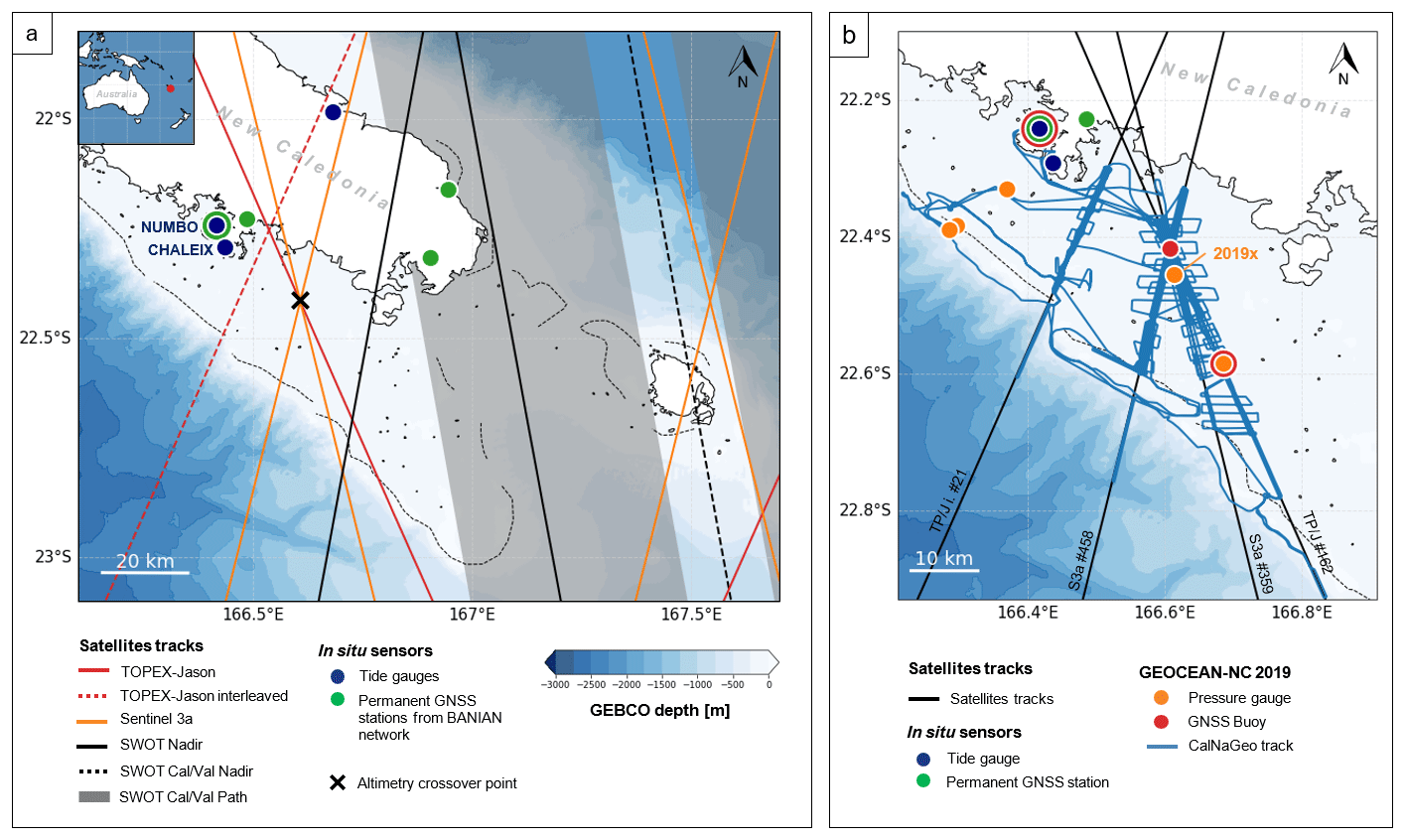
Figure 1 (a) Map of the Nouméa lagoon in the South Pacific Ocean and localisation of the main altimetry tracks and in situ sensors. The bathymetry from the GEBCO global model (GEBCO Compilation Group, 2020) is represented by a blue gradient, and the dotted lines represent the coral reefs. The black cross highlights the altimetry crossover point used in this study. In situ field campaigns will be conducted soon under the SWOT Cal/Val path. (b) Location of the sensors used (tide gauge, GNSS stations) and deployed (pressure gauge, GNSS buoy and CalNaGeo GNSS carpet) during the GEOCEAN-NC 2019 cruise. Note that some sensors were deployed at the same location: the coloured dots representing them therefore overlap.

A GNSS buoy was also successively moored at multiple locations in the lagoon (Fig. 1b, red dots), for periods of a few hours (e.g. at Numbo tide gauge) to a few days (e.g. at the crossover location). Developed by DT-INSU (Division Technique de l'Institut National des Sciences de l'Univers), it consists of a GNSS antenna (Trimble Zephyr 3) supported by a floating structure, with a metal cylinder containing the receiver (Trimble NetR9) and batteries (see picture in Fig. 3). GNSS buoys are commonly used for Cal/Val activities (Born et al., 1994; Watson et al., 2011; Bonnefond et al., 2013; Zhou et al., 2023), and many studies have demonstrated their capability to provide sea level records with centimetric accuracy (André et al., 2013; Gobron et al., 2019). During the campaign, a calibration session was performed at the Nouméa Numbo tide gauge to assess the performance of these GNSS instruments. Our results show that, despite vertical biases (−1.7 ± 0.5 cm for the buoy and −0.6 ± 0.4 cm for CalNaGeo) that could result from terrestrial geodesy measurements uncertainties and GNSS processes, these two instruments are consistent with the radar gauge observations (more details in Chupin et al., 2020).

During the campaign, five pressure sensors (Seabird SBE26plus) were moored in the lagoon at depths ranging from 12 to 20 m (Fig. 1b, orange dots). All sensors recorded pressure variations at the seafloor between October 2019 and November 2020. Three of them were installed along a profile linking the Nouméa tide gauge and the outside border of the coral reef, with the aim of quantifying the setup induced by wind and waves. Two other gauges were deployed along the TOPEX–Jason altimetry track 162 for the purpose of aiding analysis of altimeter data. Before and after their deployment, a calibration phase in a hyperbaric chamber was undertaken to check the proper functioning and overall drift of the gauges (detailed results are available in Appendix B).

Taking advantage of all observations acquired as part of the GEOCEAN-NC cruise, we thus develop a method to reconstruct a long-term virtual in situ sea level time series at the altimetry crossover point (see the black cross on Fig. 1a).

3 Reconstruction of a long-term virtual in situ sea level time series under the altimetry tracks

3.1 Method

The objective of our analysis is to compare the offshore altimetry measurements at the Jason–Sentinel-3A crossover with in situ observations. For that, two methods can be adopted (Bonnefond et al., 2011): an indirect comparison, where the in situ measurement is distant from the altimetry pass (typically a coastal tide gauge), and a direct comparison, where in situ sea surface height (SSH) is directly observed at the comparison point with instrumented platforms (as in Harvest Cal/Val site) or precise GNSS buoys. Following the method of Watson et al. (2011), we developed a mixed approach using both in situ measurements from the GEOCEAN-NC campaign and the Nouméa tide gauge records.

Figure 2 summarises the three steps of this method, which are detailed in the following sections:

•  

  Step 1. The GNSS buoy deployed at the altimetry crossover point during the GEOCEAN-NC cruise provides SSH in the same reference system as the altimetry measurements (see Sect. 3.2 for more details).

•  

  Step 2. To extend the comparison, we use measurements from the pressure sensor closest to the altimetry crossover (hereafter named the 2019× pressure sensor). By computing the mean offset between the GNSS buoy and this pressure gauge over common observation periods, the 2019× pressure sensor observations are linked to a global reference frame and virtually transferred to the altimeter comparison point (see Sect. 3.3 for more details).

•  

  Step 3. Finally, the SSH time series from the Nouméa tide gauge site is used to increase the comparison duration. Using its common year of observation with the 2019× pressure gauge, the tide gauge is virtually transferred to the crossover location by computing a tidal and datum correction (see Sect. 3.4 for more details).

3.2 GNSS buoy sea level measurements

During the campaign, a GNSS buoy was moored at multiple locations in the lagoon (see Sect. 2.2) and the first step of the data analysis concerns the measurement session during 3 d at the altimeter crossover point (Step 1 in Fig. 2). The processing of these data is essential as it constitutes the basis for the absolute attachment of our in situ observations. In that sense, all errors related to GNSS processing or the application of sensor bias will directly affect the comparison with the altimeter measurements. In particular, it is important to keep in mind that during the calibration session with the Numbo tide gauge, we found a bias of 1.7 cm with the tide gauge which is not yet fully understood (more details in Chupin et al., 2020).

The kinematic processing of the GNSS data was carried out with the GINS software, a scientific GNSS software (Marty et al., 2011), using the precise point positioning (PPP) mode. Developed in the 1990s, this method makes it possible to determine a point position without using a reference GNSS base (Zumberge et al., 1997), and recent improvements of GNSS processing allow the computation of the height of a GNSS buoy with a centimetric accuracy (Fund et al., 2013). The 10 s buoy observations (i.e. one observation every 10 s) are processed with GINS PPP mode with the integer ambiguity resolution option (details on the processing option in Appendix C, Table C1).

The resulting sea level time series is expressed with respect to the IGSR3 reference system, which is used to make the REPRO3/MG3 orbital clock products. There are no translations or rotations vs. ITRF2014, only a time-dependent vertical scale that could be approximated by +7.9 +0.19 (t−2010) mm. The distance from the GNSS antenna reference point (ARP) to sea level was determined using buoy dimensions and ruler readings during static sessions in Nouméa harbour. By subtracting all these corrections from the initial time series, we obtain the water level relative to the IAG-GRS80 ellipsoid. After a first data selection to keep positions determined with more than 10 satellites and remove outliers, the resulting heights are filtered using a Vondrak filter with a 30 min cutoff frequency (Vondrak, 1977) (Fig. 3). This filtering led to a SSH time series cleaned from high-frequency signal (e.g. short waves) (Step 1 in Fig. 2), adequate for a comparison with a 20 m depth bottom pressure records (Step 2 in Fig. 2).

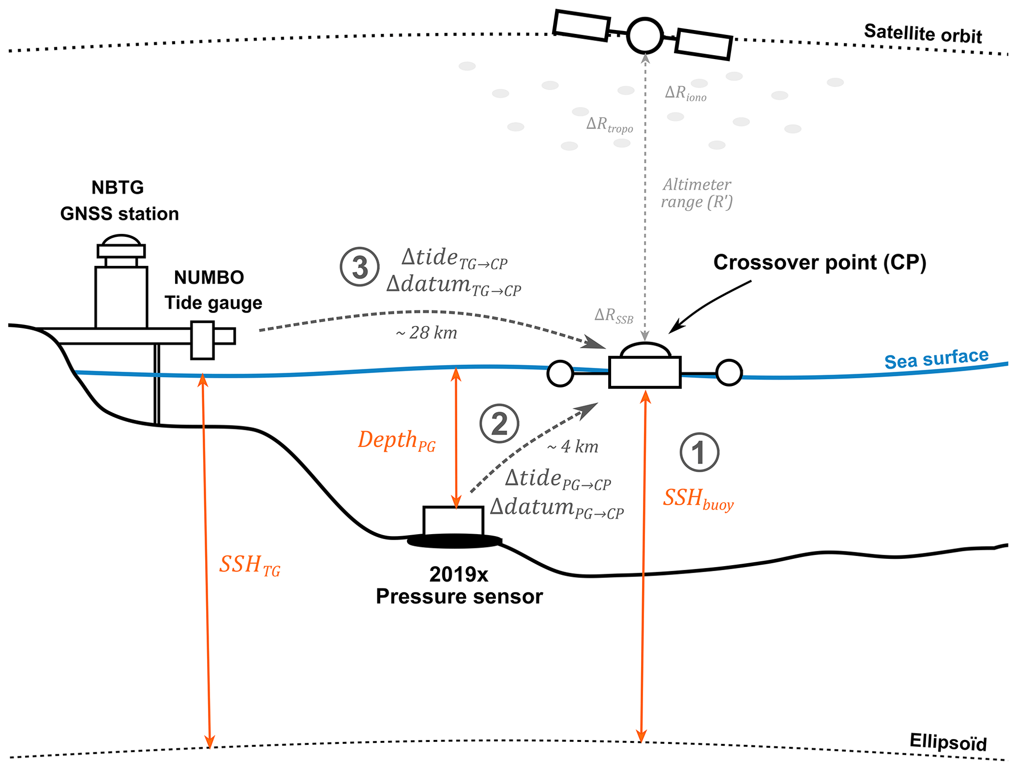
Figure 2 Configuration of the sensor's deployment. They are used to derive a long-term in situ sea level time series under the altimetry tracks. The three steps of the methodology are represented by the circled numbers.

During the buoy deployment, the area was overflown by the Sentinel-3A satellite on its track 359, which allows a direct comparison with the buoy measurements. At the time of the overflight, the SSH difference between the filtered buoy time series and altimetry measurements is about 1.4 cm (Fig. 3). As this single comparison remains limited, we then use the 1-year pressure sensor observations to extend the time series of in situ measurements.

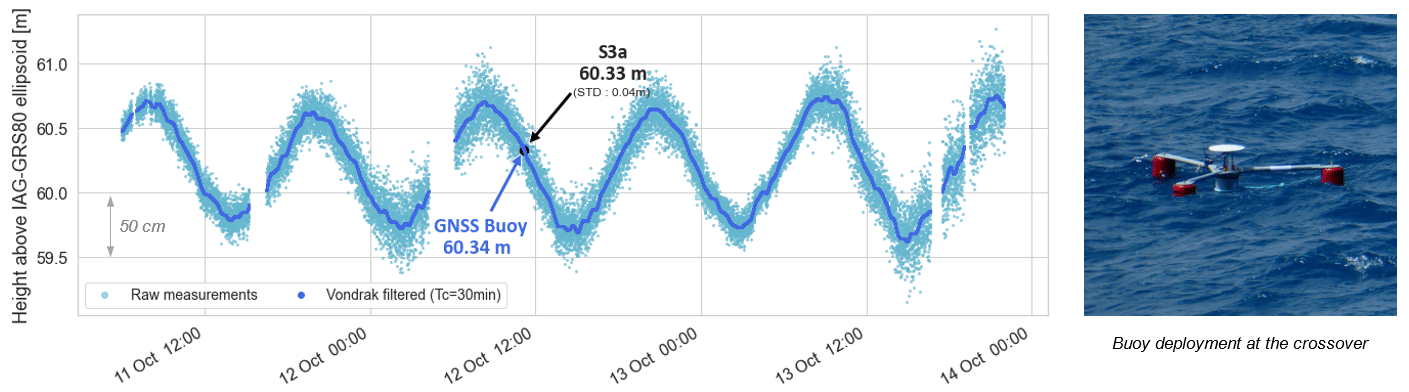
Figure 3 GNSS buoy raw (light blue) and Vondrak-filtered (dark blue) sea level heights above the IAG-GRS80 ellipsoid. The black point represents the Sentinel-3A (S3a) SSH measurement at the time of the overflight.

3.3 Pressure sensor observations

To extend the comparison, we used the 1-year pressure gauge 2019× time series. The pressure gauge deployment site, located about 4 km south of the Sentinel-3A and Jason-series crossover (Fig. 1b, orange dot), was chosen as a compromise between distance to the tracks intersection and the depth limitation of the SBE26plus (20 m). An analysis of the significant wave height (SWH) from both sensors shows that, despite the distance, they roughly monitor the same sea state (details of this analysis are shown in Appendix D). Thanks to the SCHISM hydrodynamic model output (Zhang et al., 2016), we also highlight a remaining tidal gradient between the two sensors that could reach ± 1 cm in amplitude (see Appendix D for more details). When looking at the centimetric level, this must be considered: in the following, we then apply this tidal gradient to the pressure gauge observations to be in line with the crossover tidal regime (Δtide_PG→CP in Fig. 2, Step 2).

We then used the GNSS buoy observations to tie the pressure gauge measurements into the same reference frame as the altimetry data (Δdatum_PG→CP in Fig. 2, Step 2). The 2019× seafloor pressure is converted to equivalent hydrostatic heights, using atmospheric pressure time series from ERA5, the latest climate reanalysis produced by ECMWF (Hersbach et al., 2018), at the pressure gauge location, and the water column density computed with the pressure gauge temperature and a mean salinity value of 35.5 psu. The calibration phase of the 2019× sensor shows a linear trend of about −70 mm yr⁻¹ (more details in Appendix B), which is removed to obtain the final sea level time series from the 2019× pressure sensor.

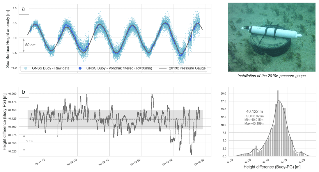
Figure 4 Comparison between GNSS buoy and 2019× pressure gauge observations. (a) Sea surface height anomaly from GNSS buoy raw data (light blue), GNSS buoy filtered data (dark blue), and 2019× pressure sensor (grey). (b) Difference between filtered GNSS buoy and 2019× pressure gauge heights. The dotted grey line represents the mean difference (40.122 m), and the grey area represents the ± 1 standard deviation (3 cm). These differences are also shown on the lower-right histogram.

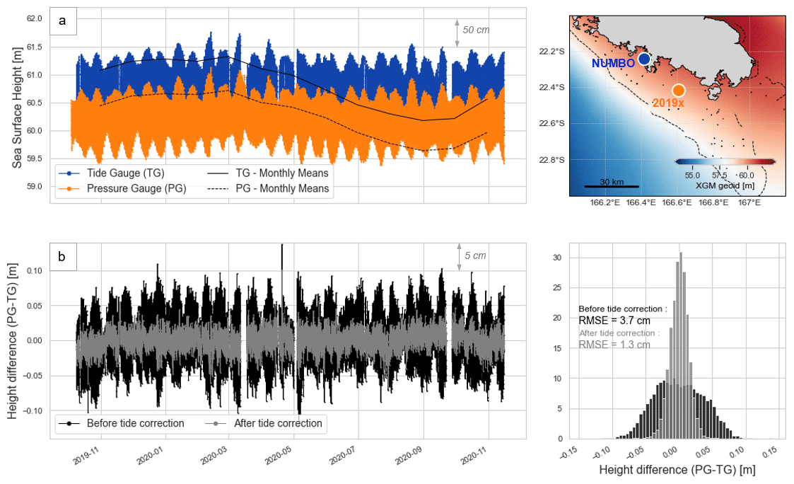
Figure 5 Tidal difference between the Nouméa tide gauge (TG) and the 2019× pressure gauge (PG). (a) Sea level record at 2019× pressure gauge (orange) and Numbo tide gauge (blue) during the common observation period (13 months). Monthly means are displayed in black (solid line for tide gauge, dotted line for pressure gauge). The two sensors are separated by about 28 km. (b) Height difference between PG and TG before (black) and after (grey) applying the tidal correction. These differences are also displayed on the histogram, with root mean square error (RMSE) values for both solutions.

The pressure gauge data are then tied to the ellipsoid by differencing the filtered GNSS buoy heights (Fig. 4a, dark blue) from the pressure sensor measurements (Fig. 4a, grey line). Over the 64 h of common observation period, the average difference is equal to 40.122 m (SD = 0.029 m – Fig. 3b). Added to the hydrostatic heights of the pressure sensor, this offset allows us to obtain a 1-year sea level record at the intersection of the altimeter tracks, hereafter named SSH_PG (Step 2 in Fig. 2). However, to have a longer in situ time series, we also considered the Nouméa tide gauge dataset (Step 3 in Fig. 2).

3.4 Nouméa tide gauge long-term measurements

The French Hydrographic Service (Shom) provides sea level observations at Nouméa through the Chaleix (operating from 1957–2005) and Numbo (2005 to present) tide gauges (Fig. 1a, blue dots). Before 1967, measurements were paper records, and electronic observations began in 1967. Thanks to a 6-month overlap of data collection, the old Chaleix site has been linked to the new Numbo site, located about 6 km away (Fig. 1a, blue dots). Aucan et al. (2017a) were thus able to reconstruct the whole time series by concatenating data from 1957–2018, making it one of the longest series available in the South Pacific. In this paper, we used the data available online (http://uhslc.soest.hawaii.edu/data/, last access: 18 July 2023 – ID 019) and regularly updated with the latest measurements from Numbo tide gauge. This 1 h sampling sea level time series will be referred to as SSH_TG in the following and covers the entire altimetry period and our study (1967–2021).

The Nouméa tide gauge and the altimeter crossover point are separated by about 28 km. The last step of our methodology is to bring tide gauge observations at the comparison point (CP), which in our study referred to the GNSS buoy location (Step 3 in Fig. 2). For that, we consider the height residuals between 2019× pressure sensor and Nouméa tide gauge measurements and compute a tidal and datum correction, as made by Watson et al. (2011) at the Bass Strait Cal/Val site. After linearly interpolating the 10 min pressure gauge data on the 1 h tide gauge time series over their common measurement period (Fig. 5a), we compute the difference SSH_PG−SSH_TG (Fig. 5b – black). We then computed an harmonic analysis on these residuals to get the tidal gradient correction in amplitude and phase (Δtide_TG→CP) and the datum correction (Δdatum_TG→CP) to apply on the tide gauge record. Tidal residuals are mainly due to semi-diurnal waves, with a contribution from M2, S2, and N2 of about 4.5, 1.7, and 1.1 cm respectively. The resulting datum correction is estimated to be −57.1 cm, which is coherent on the order of a few centimetres with gradients from two global gravity field models in the area (see Table F1 in Appendix F). After applying the tidal gradient and the datum offset, the difference SSH_PG−SSH_TG has a root mean square error (RMSE) of 1.3 cm (Fig. 5b – grey), to compare with the 3.7 cm without these corrections.

Finally, we obtain an hourly in situ sea level time series (hereafter named SSH_{in situ}) at the altimeter comparison point by virtually transferring the Nouméa tide gauge observations at the GNSS buoy location (Step 3 in Fig. 2):

$$\begin{array}{}\text{(1)}& {\mathrm{SSH}}_{\text{in situ}}={\mathrm{SSH}}_{\mathrm{TG}}+\mathrm{\Delta }{\mathrm{tide}}_{\mathrm{TG}\to \mathrm{CP}}+\mathrm{\Delta }{\mathrm{datum}}_{\mathrm{TG}\to \mathrm{CP}}.\end{array}$$

However, the altimeter flight over the area is for about 10 s between 1 and 3 times per month (for Sentinel-3A and Jason missions, respectively). Doing a simple linear interpolation of the hourly SSH_{in situ} at the satellite overfly time (t_sat) does not reproduce the tide evolution well. Thanks to a harmonic analysis over the tide gauge time series, we expressed the SSH_TG as a tide reconstruction at the time of the satellite flyby (hereafter named TGtide_rec(t_sat)) and add tide residuals linearly interpolated at the flyby time (i.e. TGtide_res(t_sat)). Thus, for the final comparison with altimetry data, the SSH_{in situ} from Eq. (1) could be explained as

$$\begin{array}{}\text{(2)}& \begin{array}{rl}{\mathrm{SSH}}_{\text{in situ}}\left(t_{\mathrm{sat}}\right)& ={\mathrm{TGtide}}_{\mathrm{rec}}\left(t_{\mathrm{sat}}\right)+{\mathrm{TGtide}}_{\mathrm{res}}\left(t_{\mathrm{sat}}\right)\\ & +\mathrm{\Delta }{\mathrm{tide}}_{\mathrm{TG}\to \mathrm{CP}}\left(t_{\mathrm{sat}}\right)+\mathrm{\Delta }{\mathrm{datum}}_{\mathrm{TG}\to \mathrm{CP}}.\end{array}\end{array}$$

With this method, there are still inaccuracies in the determination of the sea level due to weather and local conditions, but the tide evolution is well considered.

4 Calibration and validation of altimetry measurements

4.1 Altimetry data processing

4.1.1 Jason and Sentinel-3A Geophysical Data Record (GDR)

There is a wide variety of altimetry products and sources, allowing both advanced analysis of raw altimeter data and corrections and access to sea level databases that can be used directly without further processing. As our study focused on the absolute bias of the altimeter SSH, we thus consider the official latest release of along-track products to derive altimeter sea level with the up-to-date instrumental and geophysical corrections parameters.

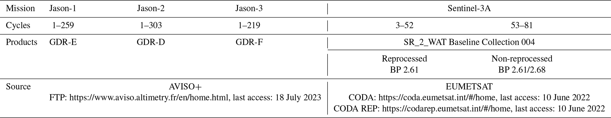
For the Jason track 162, we use the last Geophysical Data Record (GDR) delivered by AVISO+, which integrates precise orbits and up-to-date corrections for 20 Hz measurements (Table 1). For Sentinel-3A, we consider the SRAL Level-2 Marine data to ensure global coverage of the lagoon. These data are disseminated by EUMETSAT, the European Organisation for the Exploitation of Meteorological Satellites, previously on their CODA portal (Copernicus Online Data Access, until September 2022) and now on their Data Store (https://data.eumetsat.int, last access: 18 July 2023). From 2016–2019, the Sentinel-3A data were reprocessed using the current standards of the Baseline Collection 004, used for Sentinel-3A products after 2019 (Table 1).

Table 1 Altimeter products used in the study.

4.1.2 Altimetric corrections considered in order to accurately estimate sea surface height

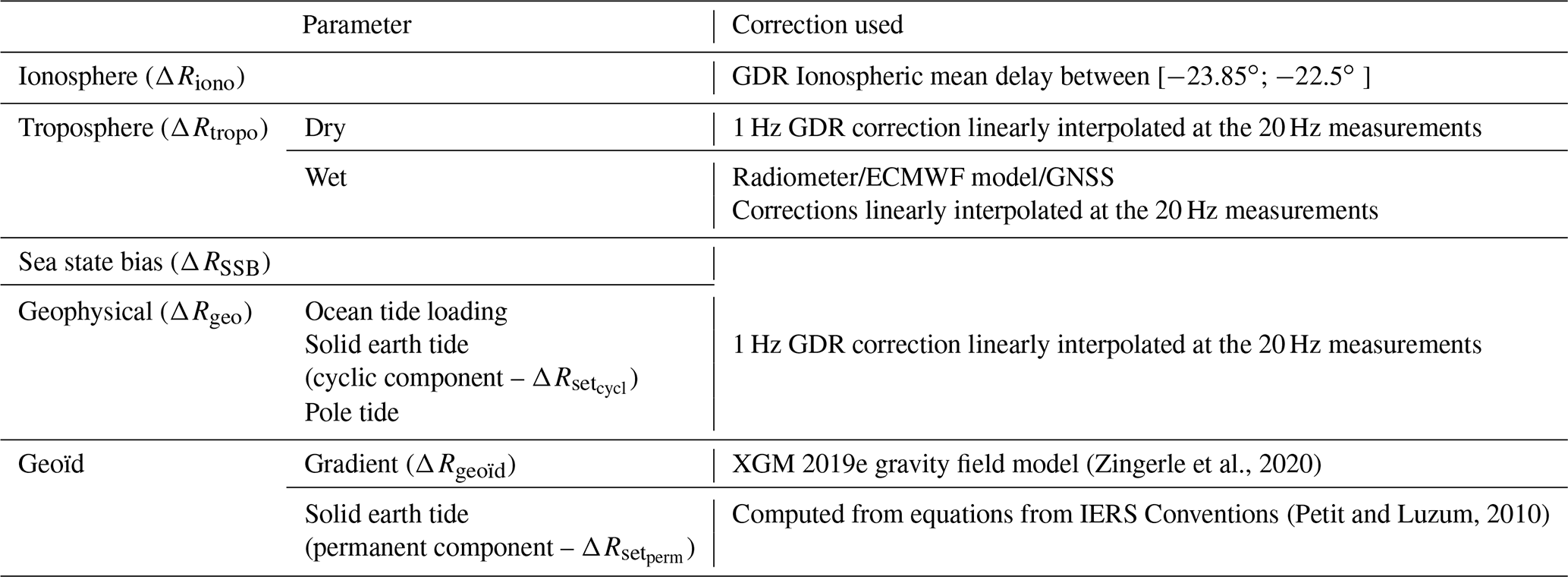
During its propagation, the radar signal is delayed by multiple phenomena that must be consider to estimate the altimetric sea surface height (SSH_alt) with a centimetric accuracy. Thus, the altimeter range must be corrected for instrumental errors (R^′), sea state bias (ΔR_SSB), and atmospheric delays (ΔR_iono and ΔR_tropo). For the comparison with tide gauge measurements, it is also necessary to integrate geophysical corrections (ΔR_geo) to account for the effect of ocean tide loading, pole, and solid earth tides.

In coastal areas, several factors can affect the quality of altimeter measurements. The proximity to the land can impact the echo received by the altimeter, which requires adapting the waveform retracking method (Gommenginger et al., 2011). The high variability of coastal processes, both in time and space, also limits the quality of atmospheric and geophysical corrections (Andersen and Scharroo, 2011). As this study is an opportunity to test different corrections in our area, we use GDR along-track products to select the most appropriate parameters or replace them by external products. In these files, the range is already corrected from instrumental errors (R^′). For our study, we also consider the ΔR_SSB and the ΔR_geo parameters at 1 Hz, linearly interpolated at the time of each 20 Hz observations (see Table 2 for a summary).

Regarding the ionospheric delay (ΔR_iono), GDR files provide a correction based on observations from the dual-frequency altimeter (Jason-3 Products Handbook, 2020) that could be very noisy. To improve this correction without degrading the altimeter measurements, one way is to smooth this ionospheric delay over a 150 km profile (Imel, 1994). Following methods developed on other historical Cal/Val sites (e.g. Watson et al., 2011), we use the mean ionospheric delay in the area between −23.85 and −22.5^∘, which covers part of the lagoon, the reef, and the open ocean, and it roughly corresponds to the recommended distance of 150 km.

The tropospheric delay (ΔR_tropo) can be divided into a wet and a dry component. About 90 % of this delay is related to the dry component, which can be estimated with atmospheric models (Chelton et al., 2001). We use the 1 Hz hydrostatic tropospheric correction provided in the GDR files, linearly interpolated to the time of the 20 Hz measurements. The wet component of the troposphere is related to the water vapour content in the atmosphere, which could be particularly variable in time and space when approaching the coast. Onboard radiometers can estimate these variations along the track. However, radiometer footprint is larger than the altimeter one (∼ 20–30 km for the radiometer and ∼ 4–10 km for the altimeter): when approaching the coast, the radiometer is thus contaminated by land earlier than the altimeter measurements (Andersen and Scharroo, 2011). In the lagoon, the effect of the land contamination is visible when approaching the main island, but at our comparison point, the radiometer correction seems to be exploitable for both Jason and Sentinel-3A missions (more details in Appendix E). To confirm this hypothesis, we also test two other datasets: (1) a wet tropospheric delay provided by the European Centre for Medium Range Weather Forecasting (ECMWF) and (2) a wet tropospheric correction computed from inland permanent GNSS stations (more details about this processing in Appendix E). When comparing with the in situ observations, we will be able to analyse the impact of these different solutions (see Sect. 4.2.1).

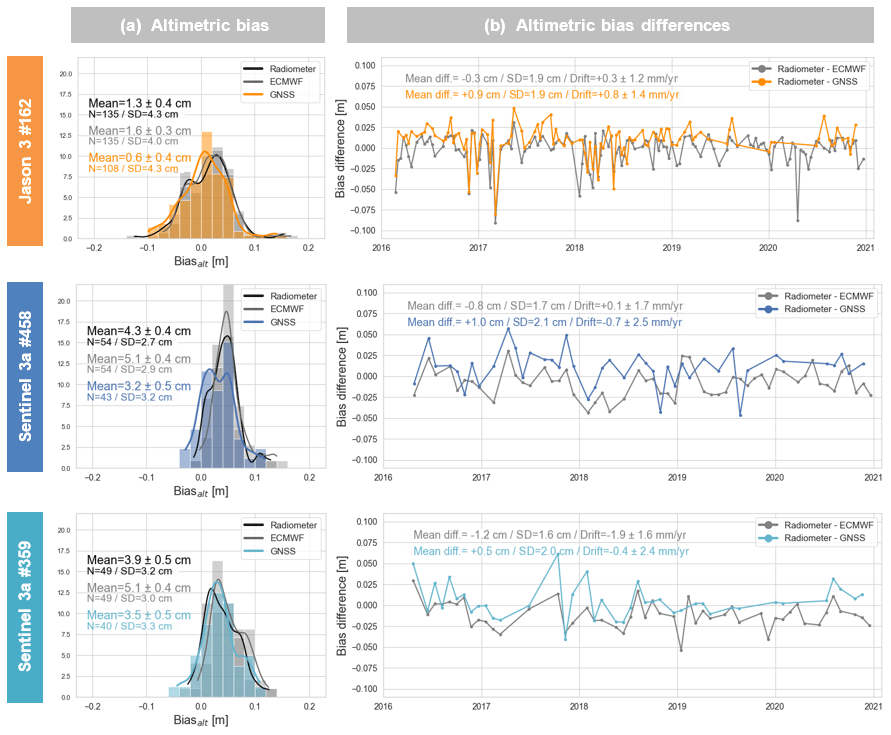
Figure 6 Altimetric bias at the comparison point according to different wet tropospheric models and for three altimetric tracks: Jason-3 (orange) track 162, Sentinel-3A tracks 458 (dark blue) and 359 (light blue). (a) Altimetric bias distribution as a function of the wet tropospheric delay from the radiometer (black), the ECMWF model (grey), and the GNSS stations (coloured). (b) Bias time differences from the radiometer solution with respect to the ECMWF model (grey) and GNSS stations (coloured).

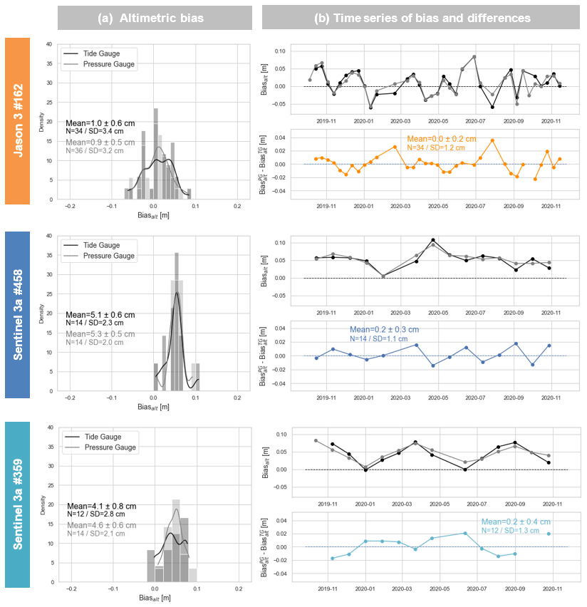
Figure 7 Altimetric bias at the comparison point according to different in situ datasets and for three altimetric tracks: Jason-3 (orange) track 162, Sentinel-3A tracks 458 (dark blue) and 359 (light blue). (a) Altimetric bias distribution using tide gauge data (black) or 2019× pressure gauge (grey) as in situ reference. (b) Bias time series using tide gauge (black) or pressure gauge (grey) as in situ dataset (upper panel) and bias time differences from the pressure sensor (lower panel).

Finally, altimetry satellites do not fly over the exact same point at each pass: it is therefore necessary to consider the height difference between the comparison point and the actual pass of the satellite track, which we approximate to be the geoid height difference (ΔR_geoïd). Using CalNaGeo observations during the GEOCEAN-NC campaign (Fig. 1b, blue lines), we demonstrate that the geoid gradients from the XGM 2019e gravity field model are the most suitable in our area (details are available in Appendix E). At each pass, we therefore use this model to determine the geoid gradient to be applied. However, in the GDR, the geoïd variable integrates the permanent component of the solid earth tide ($\mathrm{\Delta }{R}_{{\mathrm{set}}_{\mathrm{perm}}}$), while the cyclic component ($\mathrm{\Delta }{R}_{{\mathrm{set}}_{\mathrm{cycl}}}$) is included in the solid_earth_tide variable (see Jason-3 Products Handbook, 2020, and Petit and Luzum, 2010, for more details about this geophysical component). In our area, this permanent component reaches 3.2 cm and must be corrected in the altimeter processing for a suitable comparison with the in situ measurements.

In the end, the altimetric sea level time series at our comparison point is given by

$$\begin{array}{}\text{(3)}& \begin{array}{rl}{\mathrm{SSH}}_{\mathrm{alt}}& =H-R{}^{\prime }-\mathrm{\Delta }{R}_{\mathrm{iono}}-\mathrm{\Delta }{R}_{\mathrm{tropo}}-\mathrm{\Delta }{R}_{\mathrm{SSB}}\\ & -\mathrm{\Delta }{R}_{\mathrm{geo}}+\left(\mathrm{\Delta }{R}_{\text{geoïd}}-\mathrm{\Delta }{R}_{{\mathrm{set}}_{\mathrm{perm}}}\right).\end{array}\end{array}$$

The corrections used to derive the SSH_alt are summarised in Table 2.

Table 2 Altimetric corrections used to derive the SSH.

4.2 Altimetric bias computation

The determination of the altimeter bias (Bias_alt) consists of comparing the satellite observations (SSH_alt from Eq. 3) with the in situ measurements (SSH_{in situ} from Eq. 2) at the time of the overflight (Bonnefond et al., 2011):

$$\begin{array}{}\text{(4)}& {\mathrm{Bias}}_{\mathrm{alt}}={\mathrm{SSH}}_{\mathrm{alt}}-{\mathrm{SSH}}_{\text{in situ}}.\end{array}$$

At each pass, we therefore subtracted the SSH_{in  situ} from 20 Hz SSH_alt. All measurements within ± 1 km (about ± 0.17 s) from our comparison point are averaged to obtain a mean bias and an indicator of the altimeter bias dispersion. This method does not follow the standard approach used in Cal/Val sites, which consists in interpolating all corrections at the point of closest approach (PCA) (Bonnefond et al., 2011; Watson et al., 2011). However, our method allows us to reject cycles where the standard deviation of the mean bias is greater than 10 cm. In the GDR, we have also collected the range mean quadratic error (MQE) parameter. In the altimetry process, the retracking step allows the determination of the range by fitting a theoretical model on the radar echo recorded by the altimeter. We thus have access to a metric to assess the quality of the radar echo retracking result: the closer the MQE is to zero, the better the chosen model reproduce the measured waveform. With our methodology, we thus have access to the mean MQE value over the ± 1 km around the comparison point. After analysing MQE values on along-track data (more details in Appendix G), we decide to remove cycles where the MQE average exceeds the threshold value of 0.01. Finally, we apply a basic outlier detection algorithm based on the interquartile range method on the bias time series.

4.2.1 Impact of the wet tropospheric correction

To determine the most appropriate solution for the wet tropospheric correction, we compute variants of the altimeter absolute bias for Jason-3 track 162 and the two Sentinel-3A tracks over the 2016–2021 period, only changing the wet tropospheric parameter (see Sect. 4.1.2 for more details). Figure 6 represents the altimetric bias at the comparison point by using the wet tropospheric correction from the radiometer (black), the ECMWF model (grey), and the GNSS-based solution (coloured). It is important to note that the GNSS correction is not available for all cycles, unlike the radiometer and model ones that are directly taken from the GDR files.

For all missions, the resulting mean bias estimates could vary at the centimetric level depending the correction used, and the GNSS-based corrections seem to slightly decrease the value of the mean altimeter bias. The radiometer and the model agree well for the Jason-3 mission (mean difference of 0.3 cm), whereas for Sentinel-3A track 359, the radiometer seems closer to the GNSS estimates (mean difference of 0.4 cm). For both Jason and Sentinel-3A missions, none of these three corrections significantly improves the mean bias dispersion. When analysing the along-track values of the three wet tropospheric corrections (see Appendix E), we can see that they all can be very variable according to the cycles.

In any case, there is no evidence that the radiometer correction may be wrong within our study area. These results confirm that the latest improvements in radiometer corrections now included in the GDR files can be used to derive a consistent altimeter bias. A similar conclusion was made by Bonnefond et al. (2019) at the Corsica historical Cal/Val site for Jason missions. Since GNSS data are not available for all cycles, we chose to keep the wet tropospheric radiometer correction in the following analyses.

4.2.2 Evaluation of the in situ SSH determination method

To evaluate our methodology for the SSH_{in  situ} reconstruction, we compared the mean bias estimated using the 2019× pressure sensor measurements with the one computed using our method (i.e. Eq. 1) over their common observation period (from October 2019 to November 2020). Figure 7 shows the evolution of the altimeter bias for the Jason and Sentinel tracks according to the in situ data considered. For the three tracks, the difference between the mean biases is a few millimetres (+1, +2, and +5 mm for tracks 162, 359, and 458). However, we could observe centimetre level variations in the time series of differences (lower right panels, coloured curve). Despite the use of tidal gradients to integrate differences due to hydrodynamic effects in the lagoon, some variability may still exist between the location of the tide gauge and the pressure sensor. Although it is important to take this effect into account for long-term comparisons, we can still assume that the use of the tide gauge series does not affect the estimate of the mean altimeter bias. Our tide gauge data transfer method seems to be relevant for estimating the altimeter bias at the centimetre level.

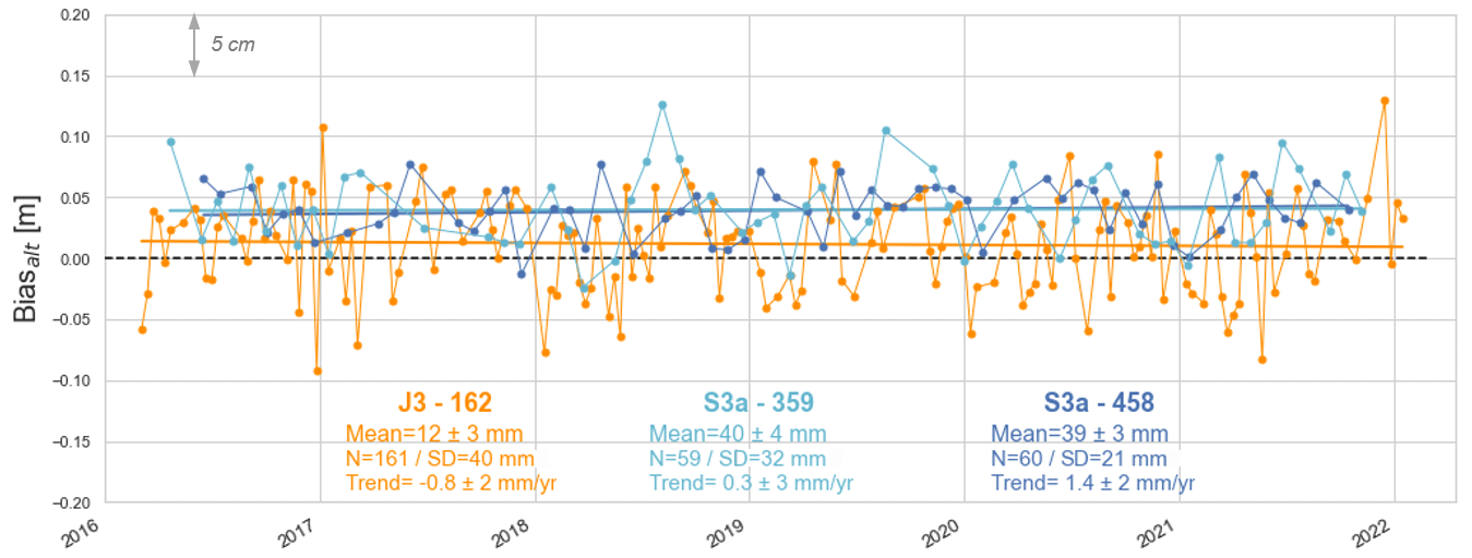
Figure 8 Altimeter bias time series at the comparison point for Jason-3 track 162 (orange) and Sentinel-3A tracks 458 (dark blue) and 359 (light blue) during their common flying period.

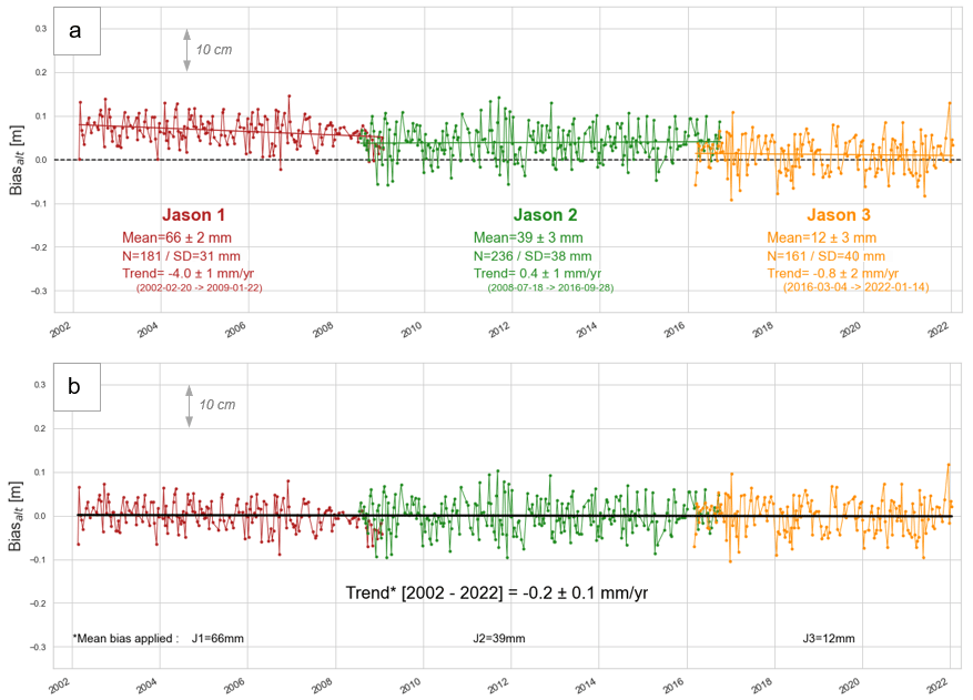
Figure 9 (a) Altimeter bias time series at the comparison point for Jason-1 (red), Jason-2 (green), and Jason-3 (orange) track 162. (b) Altimeter bias time series after applying mean biases found in this study (i.e. −66 mm for J1, −39 mm for J2 and −12 mm for J3). The black line represents the resulting trend computed over the whole Jason period (2002–2022).

4.2.3 Multi-mission comparison

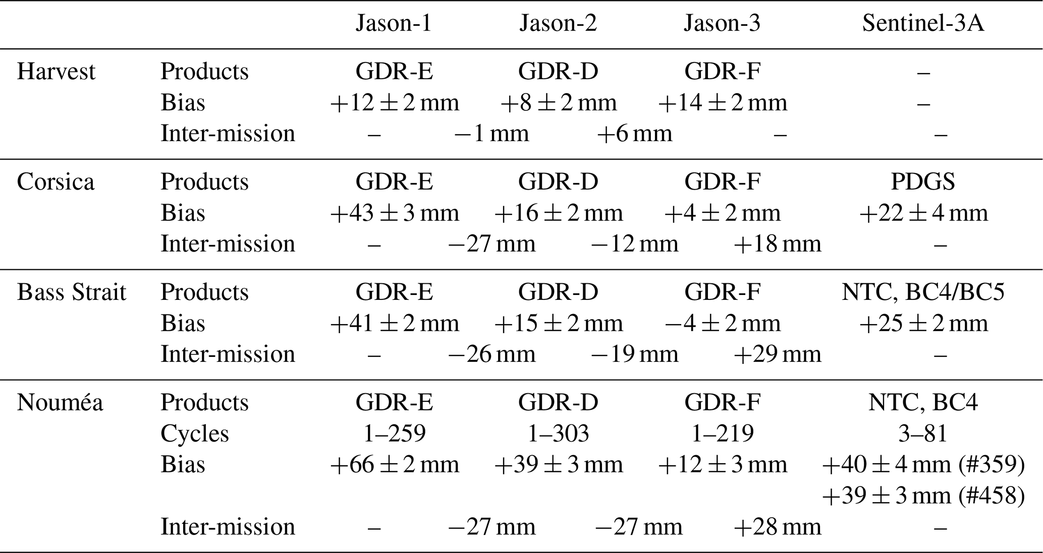
Over the period 2016–2022, both Jason-3 and Sentinel-3A measured sea level at our crossover point, which allows a direct inter-mission comparison. Figure 8 shows the altimetric biases time series for Jason-3 (mean bias of +12 ± 3 mm, orange line) and Sentinel-3A tracks 359 (+40 ± 4 mm, light blue line) and 458 (+39 ± 3 mm, dark blue line) at our comparison point. Table 3 summarises the last results of the three historical Cal/Val sites from the last Ocean Surface Topography Science Team (OSTST) meeting (Bonnefond et al., 2022a). For Jason-3, our mean bias estimate is close to the Harvest one (2 mm lower) and slightly higher than the Corsica (by +8 mm) and Bass Strait results (by +16 mm). For Sentinel-3A, we find a mean bias larger of about +16 mm compared to the Corsica and Bass Strait sites. Regarding the inter-mission bias ${\mathrm{Bias}}_{\mathrm{alt}}^{\mathrm{S}\mathrm{3}\mathrm{a}}-{\mathrm{Bias}}_{\mathrm{alt}}^{\mathrm{J}\mathrm{3}}$, we find a difference of +28 mm, which is in line with those determined at Bass Strait (+29 mm) and Corsica (+18 mm) sites (see Table 3).

The consistency of these results suggests that our methodology is suitable for estimating absolute biases. However, one must remember that uncertainties may remain in the determination of the SSH_{in  situ}. In this study, the absolute referencing of the in situ data is based on the 3 d of the GNSS buoy mooring, and many factors can influence these results at the centimetric level. These include the choice of the GNSS processing parameters, inaccuracies related to the integration of sensors biases or reference system changes, and the effect of the tether tension on the buoyancy as demonstrated at the Bass Strait site (Zhou et al., 2020). One needs to remember that, during the buoy calibration session, we found a bias of 1.7 cm with the tide gauge, which is not yet fully understood (Chupin et al., 2020). Besides, although we show that our tide gauge data transfer method is relevant (see Sect. 4.2.2), there may remain some unaccounted-for dynamic processes between the tide gauge and the comparison point that may lead to inaccuracies. To consolidate the vertical datum, new geodesy measurements with a good calibration session should be conducted to reduce uncertainties in the SSH_{in  situ} estimation and better constrain the altimeter biases.

Table 3 Altimetric mean biases and inter-mission biases for Jason-1–3 and Sentinel-3A missions for three historical Cal/Val sites and the Nouméa lagoon (Harvest, Corsica, and Bass Strait results are extracted from the last OSTST sessions – Bonnefond et al., 2022a). PDGS denotes products distributed by the Payload Data Ground Segment (ESRIN), and NTC indicates non-time-critical products from Copernicus data service.

4.2.4 Long-term altimetric bias evolution

Thanks to the long-term measurements of the Nouméa tide gauge, we compute the Jason altimeter bias time series between 2002 and 2022. The absolute bias estimates are detailed in Fig. 9a for Jason-1 (with a mean bias of +66 ± 2 mm), Jason-2 (+39 ± 3 mm), and Jason-3 (+12 ± 3 mm). The Jason-1 and Jason-2 mean biases are slightly higher than in other Cal/Val studies (Table 3), with a mean difference of about +24 mm (J1) and +23 mm (J2) compared to Corsica and Bass Strait sites. Regarding the inter-mission biases, we find −27 mm for ${\mathrm{Bias}}_{\mathrm{alt}}^{\mathrm{J}\mathrm{2}}-{\mathrm{Bias}}_{\mathrm{alt}}^{\mathrm{J}\mathrm{1}}$, which is consistent with the Bass Strait estimate. For $[{\mathrm{Bias}}_{\mathrm{alt}}^{\mathrm{J}\mathrm{3}}-{\mathrm{Bias}}_{\mathrm{alt}}^{\mathrm{J}\mathrm{2}}]$, we find an inter-mission bias of −27 mm to compare with the −19 and −12 mm of Bass Strait and Corsica sites. These results are very encouraging and show the interest of the Nouméa site to conduct further Cal/Val activities. As discussed previously, a more robust referencing of the in situ data could lead to the determination of better constrained biases.

To the first order, the altimeter bias, differences between altimetry sea level variations and those seen by tide gauge (see Eq. 4) can be related to VLM at the tide gauge site (Wöppelmann and Marcos, 2016). We therefore analysed the linear trend estimated on our altimeter bias time series to compare with the vertical motions of nearby GNSS stations. A review of the GNSS stations in New Caledonia and the associated trend estimates is available in Appendix A. While we do not obtain significant trends over Jason-2 and Jason-3 periods, our results show subsidence of 4 ± 1 mm yr⁻¹ for the Jason-1 period 2002–2008. At this time, the VLM estimates at NOUM permanent GNSS station also show subsidence (e.g. a trend estimates of −2.5 ± 0.5 mm yr⁻¹ over 2000–2007 with the SONEL–ULR7 solution). However, this value varies greatly depending on the time span and the solutions considered (see Table A2 and Fig. A3), and further investigations are needed to explain this subsidence (remaining errors in the altimetry process, more robust trend estimates over this period, etc.).

As detailed in Sect. 2.2 and Appendix A, the question of long-term sea level evolution in the lagoon is not fully resolved. With the 20 years of altimeter and tide gauge differences, we are able to estimate our own trend. First, we realign the three bias time series by applying the mean biases computed in this paper (i.e. −66 mm for J1, −39 mm for J2, −12 mm for J3) (Fig. 9b). To have a more robust estimate of the trend, we then used a bootstrapping method, which consists in estimating the trend 200 times on a random sample of 85 % of the original series. Over the whole Jason period (2002–2022), we obtain a linear trend of −0.2 ± 0.1 mm yr⁻¹. It is important to note that this trend is sensitive to the biases applied: for example, using Bass Strait mean biases (i.e. −41, −15, and +4 mm instead of −66, −39, and −12 mm), we find a trend of −0.7 ± 0.1 mm yr⁻¹.

This being said, our results do not show any significant uplift in Nouméa. This differs from the conclusions of Aucan et al. (2017a), who find an uplift of 1.41 ± 0.67 mm yr⁻¹ over the altimetric period (1993–2013) inferred from the difference between satellite altimetry and tide gauge. The difference likely originates in the method used by Aucan et al. (2017a), in which the satellite altimetry time series was extracted from a multi-mission gridded dataset at a point far outside the lagoon, before being compared to the tide gauge (see Fig. A4 in Appendix A). Section 4.2.2 shows that, even being only a few kilometres apart, there is SSH differences between the tide gauge and the pressure sensor: the difference with a point outside the lagoon can therefore be even greater. Other studies that compare altimetry and tide gauges also find a significant uplift in the area (1.7 ± 0.2 and 2.5 ± 1.5 mm yr⁻¹ for Nerem and Mitchum, 2002, and Martínez-Asensio et al., 2019, respectively). By using along-track altimetry products and a closer comparison point, our approach led to a slightly different conclusion.

Regarding VLM estimates from GNSS permanent stations, one thing to note is that most of them highlight small subsidence in New Caledonia (see Appendix A). For example, thanks to the combined results of multiple computing centres, Ballu et al. (2019) found average subsidence of 1.3 ± 0.3 mm yr⁻¹ in Nouméa. However, authors also show that this VLM estimation can be very sensitive to the integration (or lack thereof) of a discontinuity in the time series. To solve the question of long-term sea level change in the lagoon, further studies are thus needed on GNSS data analysis as well as on altimetry and tide gauges. For example, extending our time series with TOPEX/Poseidon or Sentinel-6 observations would give us a longer and more robust trend estimate. Having longer observations from the GNSS permanent station collocated with the Numbo tide gauge could also help to constrain vertical land motions at the tide gauge.

5 Conclusions

In this paper, we demonstrate the potential of the New Caledonia lagoon near Nouméa to host Cal/Val activities. Using in situ data acquired as part of the GEOCEAN-NC campaign, this study proposes a method to link and compare observations from the Nouméa long-term tide gauge site and an offshore altimetry crossover point from Jason and Sentinel-3A missions. Thanks to the measurements of a GNSS buoy and a bottom pressure sensor, we are able to virtually transfer long-term Nouméa tide gauge data at this altimeter crossover. A comparison over the common year of measurement of the tide gauge and the pressure sensor shows that this method is relevant for estimating altimeter bias at the centimetre level. The use of along-track altimetry product allows us to test and adapt altimeter correction parameters, especially for the wet tropospheric delay. We consider the up-to-date GDR parameters, and thanks to a CalNaGeo survey, we validated the use of the XGM2019 gravity field model to account for geoid gradients.

Following the philosophy of Cal/Val studies, we are thus able to compute a precise absolute altimeter bias time series. For the three Jason missions and Sentinel-3A, we find mean altimeter biases slightly higher than other historical Cal/Val sites estimates, except for the Jason-3 mean bias, which is close to the Harvest one. Our estimates of the inter-mission biases are also consistent, especially with the results of the Bass Strait site (see Table 3). These results are very encouraging, despite the uncertainties about the vertical referencing of our in situ observations (see Sect. 4.2.3). Additional geodetic measurements with buoys and pressure sensors at the crossover location could help to control and consolidate this vertical datum. In the future, this site also gives the opportunity to reanalyse data from the TOPEX/Poseidon to the recent Sentinel-6 missions. Extending the comparison will allow one to answer new questions and particularly try to reconcile the sea level trends seen by altimetry, tide gauges, and terrestrial permanent GNSS stations. One could also consider transposing this method to other study areas, thus increasing the potential number of Cal/Val studies around the world. However, in addition to enabling the deployment of offshore geodetic campaigns, these potential sites require having suitable altimetry measurements in the vicinity of a reliable sea level observatory (e.g. a long-term tide gauge site) and a good knowledge of the local geophysical and hydrodynamic context to account for the difference in oceanographic signals.

Finally, although the GEOCEAN-NC campaign is not directly related to the preparation of the future SWOT mission, a better knowledge of the lagoon dynamics and the mapping of the fine-scale geoid will be useful for the exploitation of its future large-swath measurements. Thus, the Nouméa lagoon represents a real opportunity to establish an absolute and relatively low-cost Cal/Val site, to better understand current and future altimetry data.

Appendix A: Geophysical situation of the Nouméa lagoon

This appendix gives the geophysical context of our study based on the scientific literature.

A1 Global geophysical context (from Ballu et al., 2019)

Ballu et al. (2019) detail the geophysical context of the southwestern Pacific zone (see Fig. A1 for an overview). Focusing on our study area, the Nouméa lagoon is on an active tectonic zone on the Indo-Australian Plate, which converges with the Pacific one at a mean rate of about 10 cm yr⁻¹. There are two major subduction zones, and Nouméa is near the New Hebrides and Papua New Guinea–Solomon Islands one, where the Australian Plate is subducting. The contribution of non-tectonic processes to vertical displacement (i.e. subsidence of Pacific volcanoes and post-glacial isostatic adjustment) is estimated to be less than 1 mm yr⁻¹. It also appears that Nouméa could be affected by earthquakes, although neither strongly nor frequently.

Table A1 Tide gauge relative sea level trends estimates in New Caledonia from different studies.

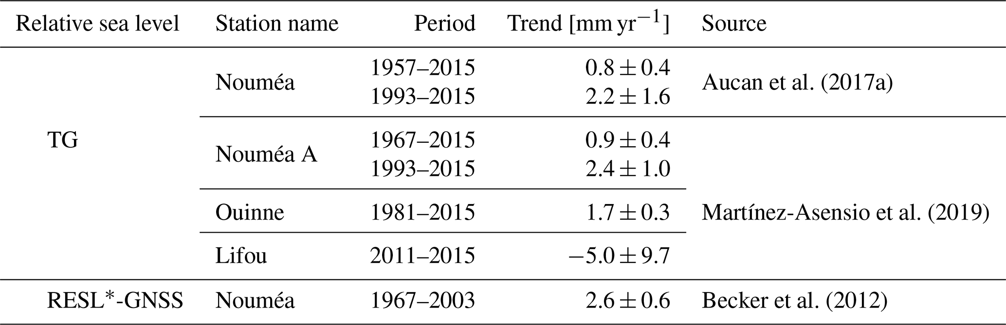
^* RESL – reconstructed sea level (see Becker et al., 2012, for more details).

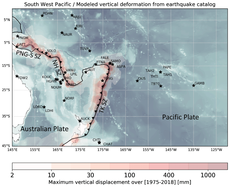
Figure A1 Extracted from Ballu et al. (2019) – stars represent stations with a long enough GPS record available (∼ 7 years). The background grey/blue shading highlights the bathymetric features in the oceanic domain, based on GEBCO 2014 (Weatherall et al., 2015) bathymetric data. The red shading indicates maximum absolute values of vertical displacement modelled using the Okada (1985) dislocation model and the USGS earthquake catalogue for the period 1975–2018. The black line corresponds to the tectonic plate limit between the Australian Plate and the Pacific Plate, as proposed in the MORVEL-25 plate boundary model (DeMets et al., 2010). The subduction zones are indicated by triangles on the over-riding plate and labelled TK SZ, NH SZ, and PNG-S SZ, respectively, for the Tonga–Kermadec, New Hebrides, and Papua New Guinea–Solomon Islands subduction zones.

A2 Global and local hydrodynamic context

There is a strong sea level regional variability in the western tropical Pacific area, mainly linked to the ENSO (El Niño–Southern Oscillation) with lower sea level during El Niño (higher during La Niña) events, with differences in sea level around ± 20–30 cm (Becker et al., 2012). From the study of Garcin et al. (2016), it appears that periods that combine La Niña events and a negative Interdecadal Pacific Oscillation (IPO) lead to stronger trade winds and higher sea levels in the lagoon. The climate component of sea level rise in Nouméa is estimated to be around +0.5 ± 0.5 mm yr⁻¹ (Becker et al., 2012).

The lagoon surrounding New Caledonia is the world's largest lagoon, covering about 20 000 km². A barrier reef separates the lagoon from the Pacific Ocean, at a distance from the coast ranging from 5 km in its northern part to 40 km in its southern part. Deep passes intersect the coral reef and let the ocean flow in and out. During low tides, the crest of the reef can emerge.

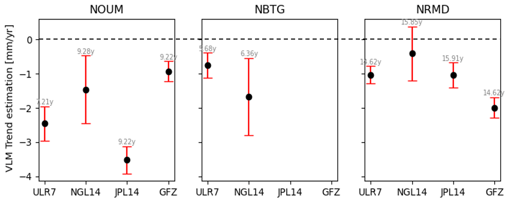
Figure A2 VLM trend estimation at three GNSS stations in Nouméa from four different solutions: SONEL–ULR7 solution from Gravelle et al. (2023), NGL–NGL14 solution from Blewitt et al. (2016), JPL–JPL14 solution from Heflin et al. (2020), and GFZ–GT3 solution from Männel et al. (2022). The red bar represents the uncertainty associated with each estimate, and the number shows the length of the observation years used to estimate the trend.

The southern part of the lagoon, near Nouméa city, has an average depth of 15–20 m. Its dynamics is dominated by semi-diurnal tides, with a tidal range varying from about 1.4 m at spring tides to 0.6 m at neap tides (Douillet, 1998). Part of the offshore oceanic signal enters the lagoon through deep passes, but it is then strongly attenuated inside the lagoon by wave breaking and friction on the reef flat (Bonneton et al., 2007).

To a first approximation, the sea state in the lagoon is mainly dominated by the wind sea (Jouon et al., 2009). Aucan et al. (2017b) identify three types of waves in the lagoon: (1) low-frequency swell waves (8–25 s) generated offshore (SSW) and then impacting the barrier reef; (2) high-frequency waves (3–8 s), generated inside the lagoon by the prevailing trade winds (SE); and (3) infragravity waves (20–500 s) that can be similarly energetic on the islet reef flat. The wave impact on the islands depends on their location and distance to the coral reef and the main passes, and it is modulated by tidal level and the surrounding reef plate (Aucan et al., 2017b; Garcin et al., 2016).

Finally, it is possible that wave breaking on the barrier reef could induce a localised elevation of the water body behind the reef (i.e. setup), which would be evacuated through the passes and would not necessarily reach the coast and thus the tide gauge. This phenomenon was observed during the passage of Tropical Cyclone Cook in 2017 (Jullien et al., 2020). However, in a previous publication based on in situ data in the lagoon (Aucan et al., 2017b), no significant setup was observed (Jérôme Aucan, personal communication, 2017).

A3 Sea level trends and vertical land motions in New Caledonia

In New Caledonia, the sea level evolution is still an issue as altimetry, tide gauge, and land-based GNSS stations do not provide consistent information (Aucan et al., 2017a; Martínez-Asensio et al., 2019; Tables A1 and A2 for an overview of the values). Over the altimetry period (1993–2013), Aucan et al. (2017a) find a sea level trend difference between tide gauge and altimetry of +1.4 ± 0.7 mm yr⁻¹. Ideally, these residuals movements could be explained by vertical land motions (VLMs). However, neither the VLM estimated by glacial isostatic adjustment (GIA) models (i.e. ∼ −0.1 to −0.3 mm yr⁻¹ in the area from the ICE6G-VM5a model – Peltier et al., 2015) nor the VLM estimation from permanent GNSS stations (Table A2) could explain the uplift inferred by altimetry minus tide gauge measurements.

Several hypotheses could be considered to explain this:

1. It could be the water level elevation between the altimeter sampling point and the tide gauge position (i.e. setup), which does not appear to be significant in the lagoon (see the previous section for more details).

2. Mismodelled discontinuities in the GNSS time series can result in an incorrect estimate of the VLM. In their comparative study of different GNSS solutions, Ballu et al. (2019) find that the estimation of the VLM trend for the NRMD station is very sensitive to the integration (or not) of a discontinuity during a material change in the middle of the time series. The methodology used to compute the trend and the period considered also impact the final result (see Table A2 and Fig. A2 for the different estimates of the VLM at GNSS stations and Fig. A3 for time series comparison at NOUM station).

3. We can also consider the processing of altimetry data. For now, the data used in the tide gauge comparison are derived from gridded products integrating standard corrections that may not be appropriate for coastal locations. In Aucan et al. (2017a), the altimeter point selected for comparison is located 95 km from the tide gauge. When considering the variability of sea level trends seen by altimetry in this area (Fig. A4), one wonders whether the selection of a point so far from the tide gauge is appropriate.

Table A2 Vertical land motion trend estimates in New Caledonia from different studies.

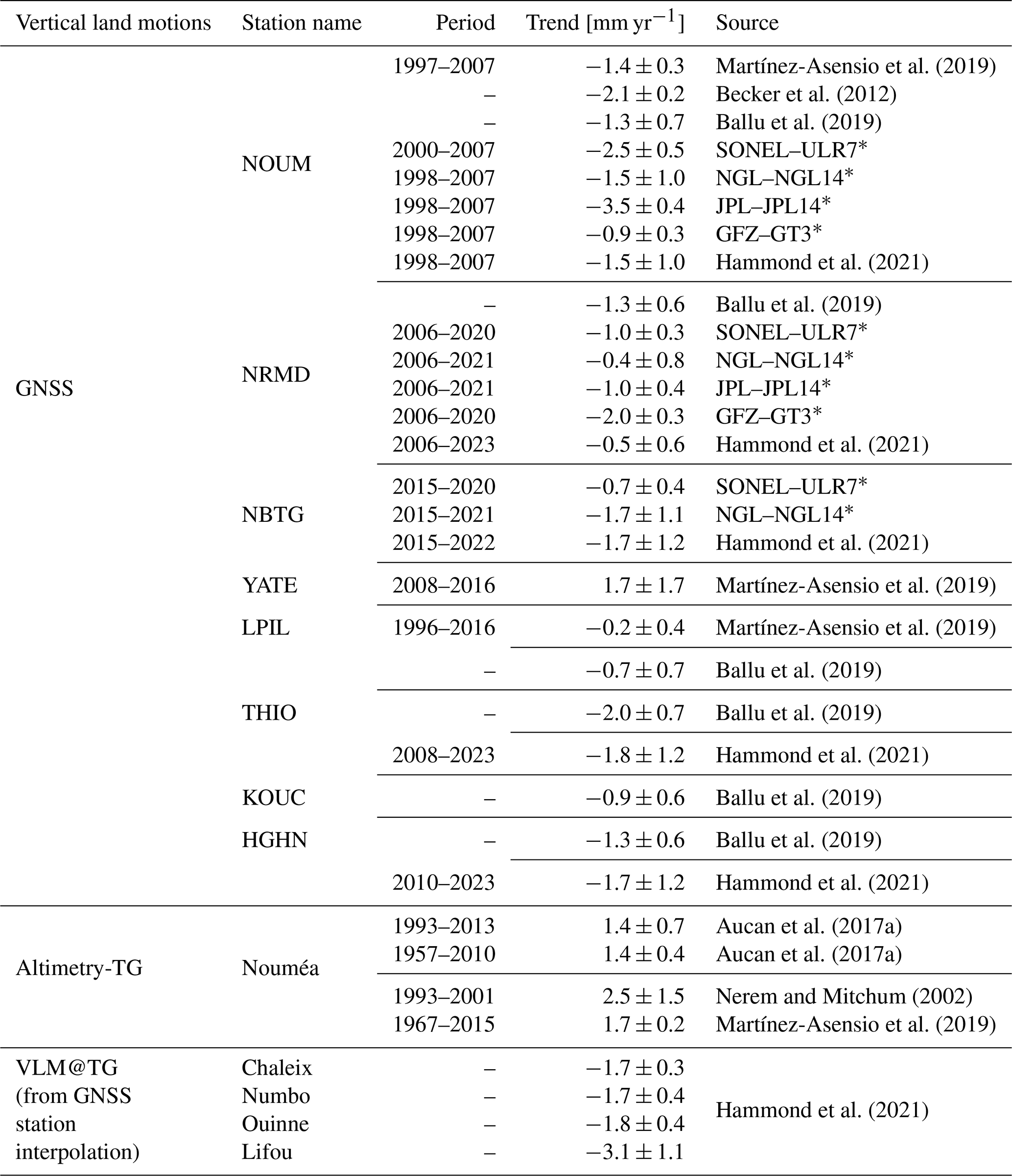
^* GNSS VLM sources: SONEL–ULR7 solution from Gravelle et al. (2023). NGL–NGL14 solution from Blewitt et al. (2016). JPL–JPL14 solution from Heflin et al. (2020). GFZ–GT3 solution from Männel et al. (2022).

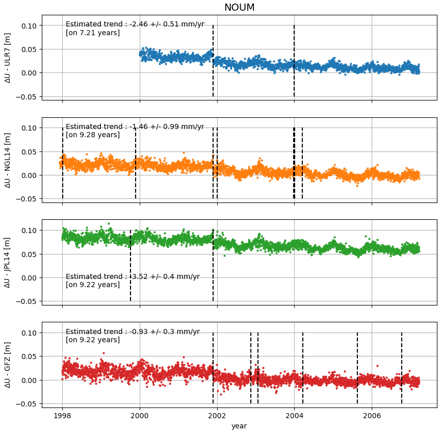
Figure A3 Time series used to estimate VLM trend at the NOUM station for the four solutions presented in Fig. G2. The dashed vertical bar indicates the discontinuity considered by each solution to compute the final trend.

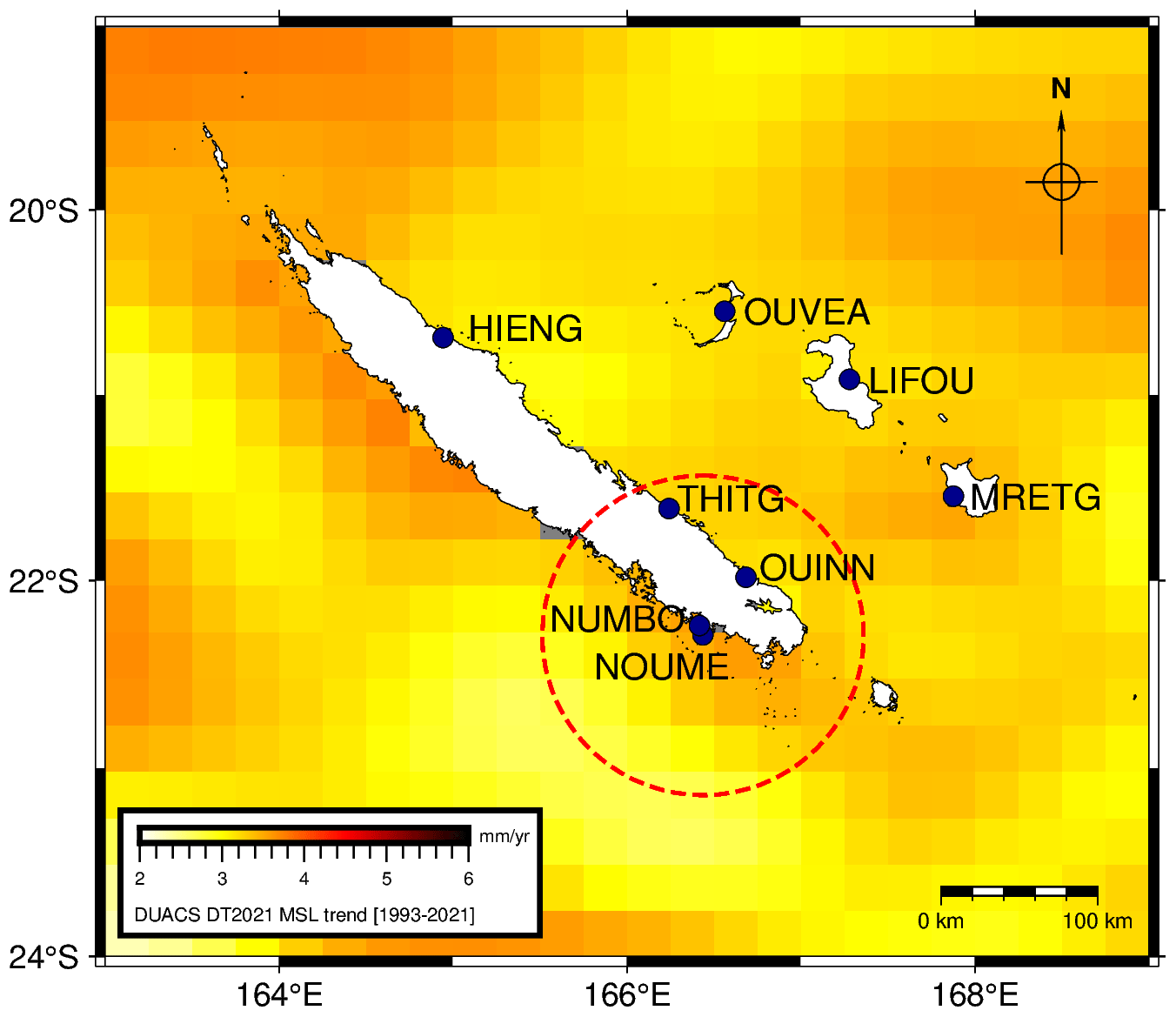
Figure A4 Location of the main TG sites in New Caledonia. The background shows the merged gridded regional mean sea level trends from DUACS DT2021 over 1993–2021 (generated using EU Copernicus Marine Service Information; https://doi.org/10.48670/moi-00238; CLS/CMEMS). The dotted red circle with 95 km radius represents the distance between Nouméa tide gauge and altimetry grid node used in the Aucan et al. (2017a) study for comparison.

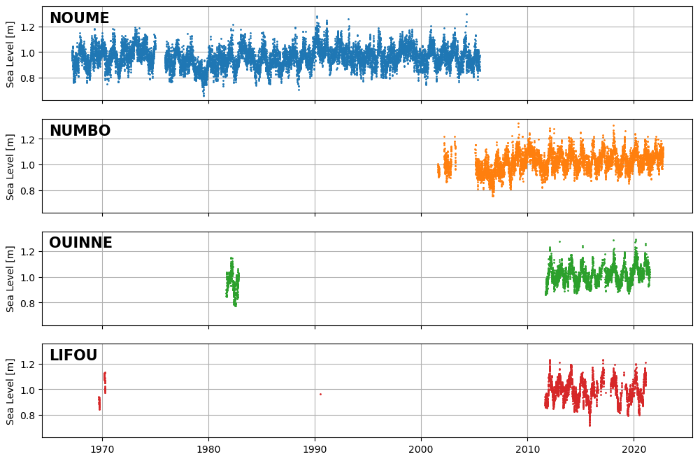
Figure A5 Overview of NOUME, NUMBO, OUINNE, and LIFOU tide gauge daily sea level means from the SONEL portal.

Appendix B: Calibration of GEOCEAN-NC pressure gauges

Pressure sensors are known to drift over time. This drift is generally considered to be linear and variable from instrument to instrument, depending on the age and past history of the sensor. In our case, a calibration session in hyperbaric chamber before and after their deployment does not show a clear instrumental drift of the different sensors (Fig. B1c).

To verify the stability of the measurements during the 13 months of immersion, we compute relative differences with the 2019o sensor (Fig. B1d). This sensor was chosen as a reference because of its installation on a stable support (coral reef), and we consider its instrumental drift negligible regarding the previous calibration session. Results show that, for sensors 2019i and 2019j (Fig. B1d, in green and yellow), differences do not show a significant trend; therefore, it is assumed that these two sensors remained stationary.

On the contrary, the 2019o–2019r difference (Fig. B1d, in red) shows a negative trend for the first 7 months, before stabilising in May 2020. This suggests a sinking of the 2019r sensor into the sand, which was confirmed by the divers during the gauge's recovery. The nature of the bottom is therefore a parameter to consider when deploying the sensors. If the experimental conditions impose an installation on very soft grounds, other types of support can also be considered (suction anchors, etc.).

Finally, the 2019o–2019× difference (Fig. B1d, blue) shows a linear trend of about −70 mm yr⁻¹, which is neither visible on the other sensors nor conceivable from the pre- and post-deployment drift checks. This could indicate continued 2019× sensor sinking, and in the absence of further information, we chose to correct for this trend in the following study.

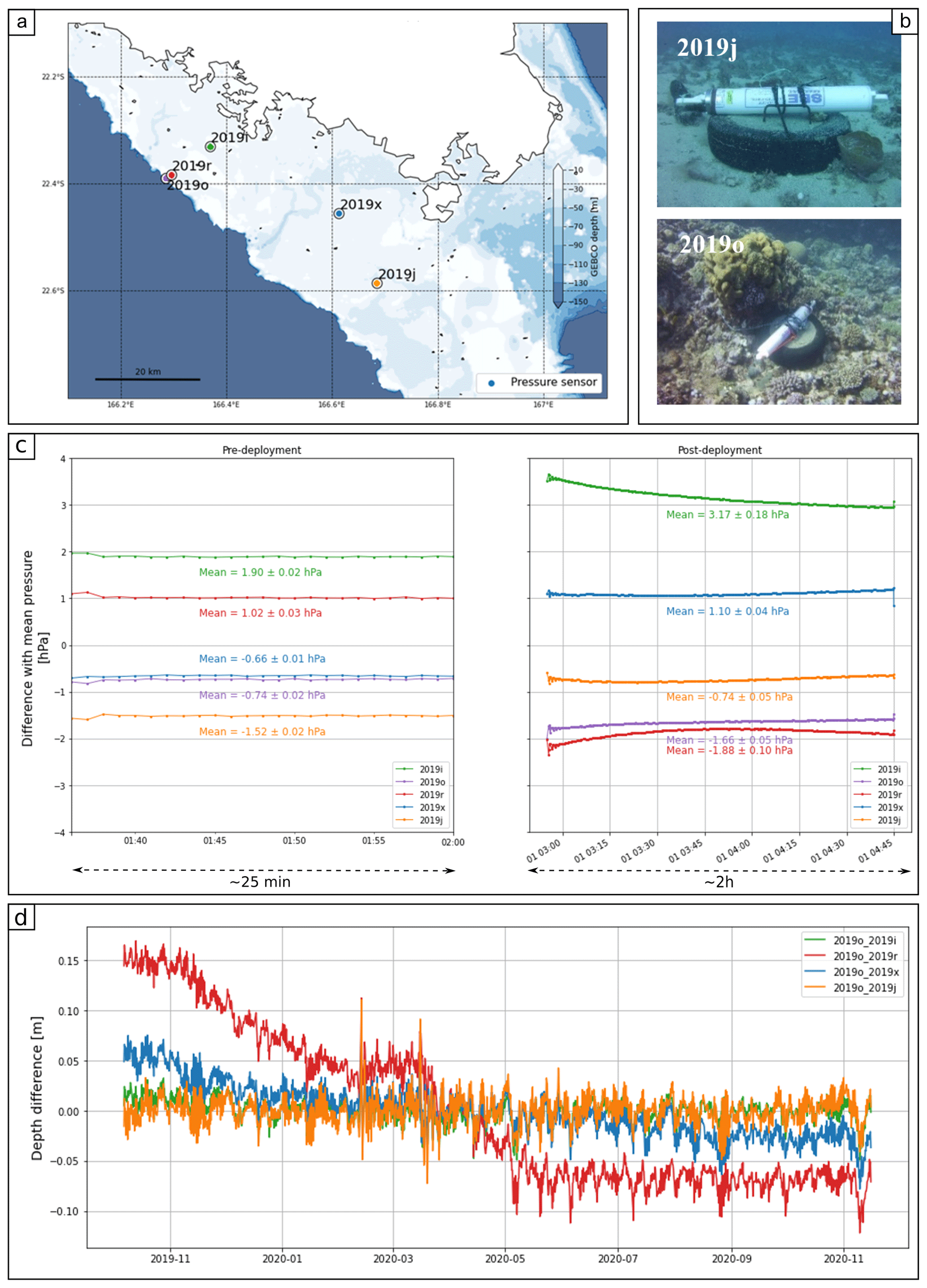
Figure B1 Installation and calibration phase of the pressure gauges. (a–b) Location and mooring of the five pressure gauges deployed during GEOCEAN-NC campaign. (c) Hyperbaric chamber calibration results: difference between Seabird SBE26plus observations and mean pressure at 10 m before (left) and after (right) deployment. For conversion, 1 hPa ∼ 1 cm of water. (d) Difference between the 2019o sensor time series and the other four pressure sensors. The pressure time series were transformed into equivalent water depths and then corrected for tide using harmonic analysis. The final differences were filtered with a sliding average (6 h windows, 6 h steps).

Appendix C: GNSS processing parameters

Table C1 GINS parameters for GNSS computation^*. IPPP indicates integer precise point positioning.

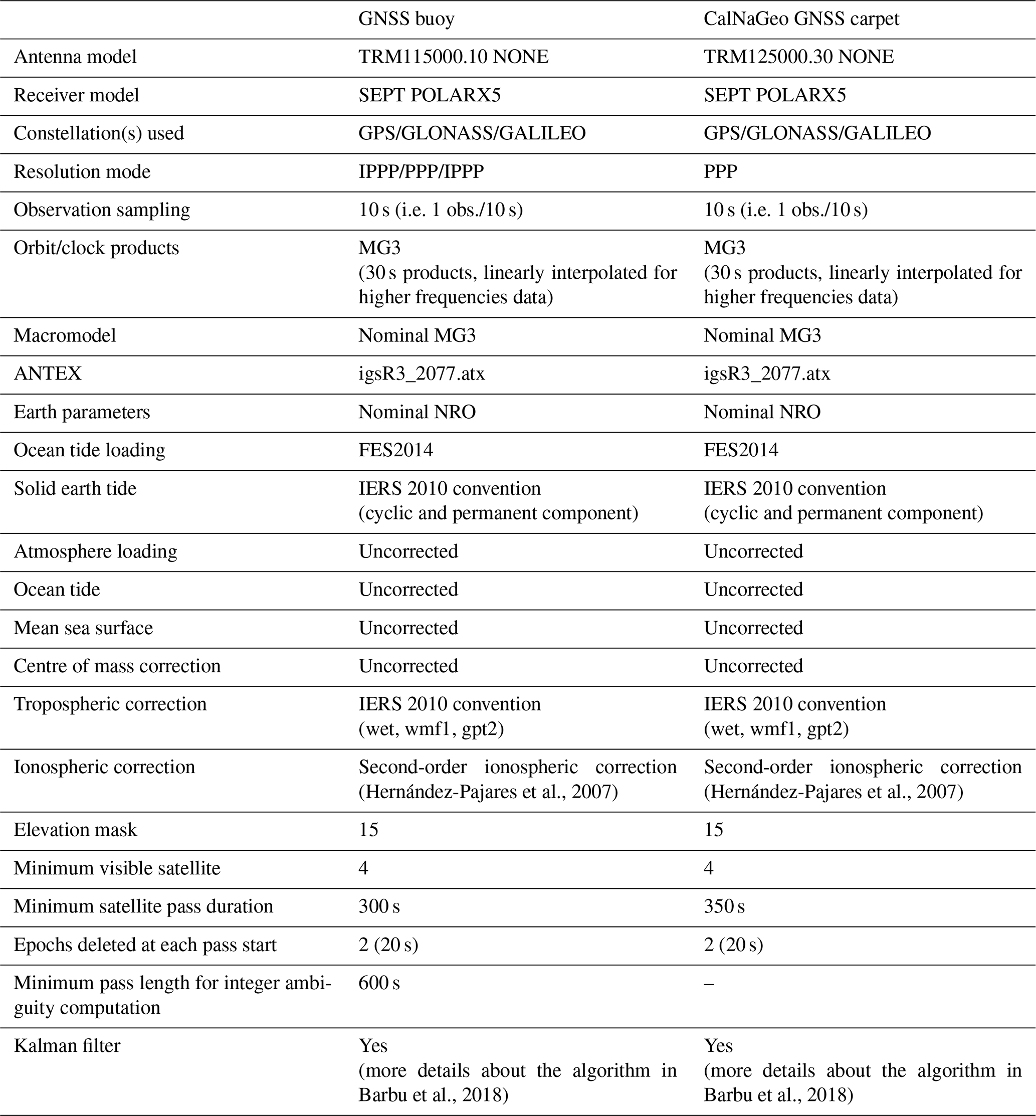
^* For more details about the GINS software, see GRGS (2018) and Marty et al. (2011). The reader may also refer to the paper of Kouba (2015) for a description of the different parameters and models that can be used in the GNSS computation process.

Appendix D: Sea state comparison between GNSS buoy and 2019× pressure sensor

To be sure that the GNSS buoy and the 2019× pressure sensor monitor the same sea, we compare the SWHs from both instruments. As they are located 4 km apart, we also used tide model predictions at both locations to compute a tidal gradient between both sensors.

D1 SWH from the GNSS buoy

Located at the water surface, the GNSS buoy observations are directly impacted by the sea state as well as by longer variations such as tide or the geoid. To process these data, we used the method describe in Bonnefond et al. (2003). To focus on the short variations, we differentiate between the filtered and the raw buoy data (RTKLIB 1 Hz differential solution). For that, GNSS heights are filtered using the Vondrak filter (Vondrak, 1977) with a cutoff period of 120 s to remove short-wavelength oscillations (Fig. D1a). Standard deviation of the residual heights (σ_shr) is computed using a 120 s period running average (Fig. D1b). The standard deviation of the buoy due to waves (σ_wave) is then equal to ${\mathit{\sigma }}_{\mathrm{wave}}=\sqrt{{\mathit{\sigma }}_{\mathrm{shr}}^{\mathrm{2}}-{\mathit{\sigma }}_{\mathrm{gps}}^{\mathrm{2}}}$ with σ_gps as an estimation of the GNSS buoy processing errors (here estimated to be 2.5 cm). The final SWH at the buoy is then derived from SWH $=\mathrm{4}\times {\mathit{\sigma }}_{\mathrm{wave}}$ (Fig. D1c).

D2 SWH from the 2019× pressure sensors

The SBE26plus sensors have been set up to measure wave bursts for 10 min every hour (with 1 s wave sample duration). To compute the resulting SWH from theses wave bursts at 2019×, we first transform pressure records to equivalent hydrostatic depths atmospheric pressure time series from ERA5 (Hersbach et al., 2018) at the pressure gauge location, temperature from the pressure recorder, and a mean salinity of 35.5 psu. Then, we remove a linear trend for each burst of 512 values and reconstruct wave elevation. The power spectrum density (PSD) is then estimated, and the final wave parameters are extracted. After several tests, we chose a cutoff frequency of F_c = 0.25 Hz. In order to easily compare with GNSS buoy SWH, this method is applied to the buoy observations, after selecting the same observation windows as from the pressure sensor's wave bursts.

D3 SWH comparison

The results of the GNSS buoy and 2019× pressure sensor SWH computation are shown in Fig. D3a. We can see that the GNSS buoy, measuring at the direct water surface, is very sensitive to waves, down to frequency bands of 0.5 Hz. If we apply the same cutoff frequency as the bottom pressure sensor (F_c = 0.25) to the buoy data, we obtain a high correlation between the two series (c=0.914, Fig. D3b). Thus, at a depth of around 20 m, the pressure sensor is limited to a narrower frequency band than the buoy. But if we limit the comparison at the frequency band common to both systems, they roughly see the same sea.

D4 Tidal gradient between 2019× pressure gauge and buoy location

Although only 4 km apart, the GNSS buoy and the pressure sensor may be subject to slightly different tidal regimes. We therefore used the output of the SCHISM hydrodynamic model, provided by Jérôme Lefevre from the IRD in Nouméa, to compute the tidal gradient between the two positions.

Figure D4 represents these results: the bar plots in the left panel show the model extraction of amplitude and phase of the main tidal constituents at the buoy (blue) and pressure sensor location (orange). Differentiating the tide constituents (PG minus buoy), we obtain the amplitude and phase of the tidal gradient (red). The tide reconstruction due to this tidal gradient is shown in Fig. D4c. We can see that over the 3 d of the GNSS buoy deployment, we could have height differences up to ± 1 cm between the buoy and the pressure gauge location.

These values are not negligible in our case, where we aim to get closer to the centimetre level. Figure D5 represents the water heights difference observed by the GNSS buoy and the pressure sensor (see Sect. 3.3 for more details), considering or not considering this tidal gradient. When comparing histograms of the residuals (Fig. D5b), we can see that adding the gradient improves the distribution of the residuals, without impacting the mean bias. We have subsequently considered this tidal gradient to correct the observations of our pressure sensor.

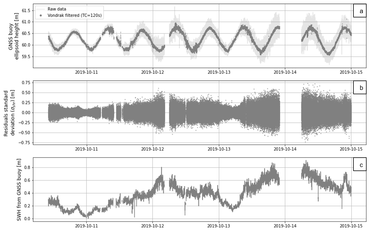
Figure D1 Computation step of the GNSS buoy SWH. (a) Raw and Vondrak-filtered GNSS buoy ellipsoid heights. (b) Standard deviation of the residual heights computed in a 120 s window (σ_shr). (c) Significant wave height (SWH) at the buoy position.

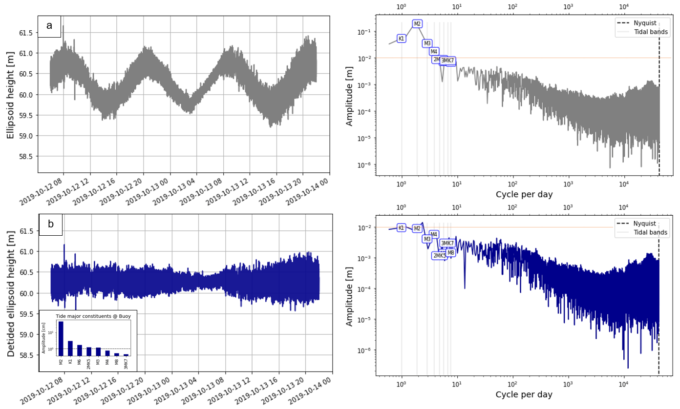
Figure D2 Fast Fourier transform (FFT) computation for GNSS buoy observations of the 12–13 October 2019. (a) GNSS buoy ellipsoid heights over the period (left panel) and its corresponding FFT (right panel). (b) GNSS buoy detided ellipsoid height (left panel) with the amplitude of the major tide constituents at the buoy location and its corresponding FFT (right panel). Note that for the two FFT plots, the dotted red line highlights the 10 cm amplitude.

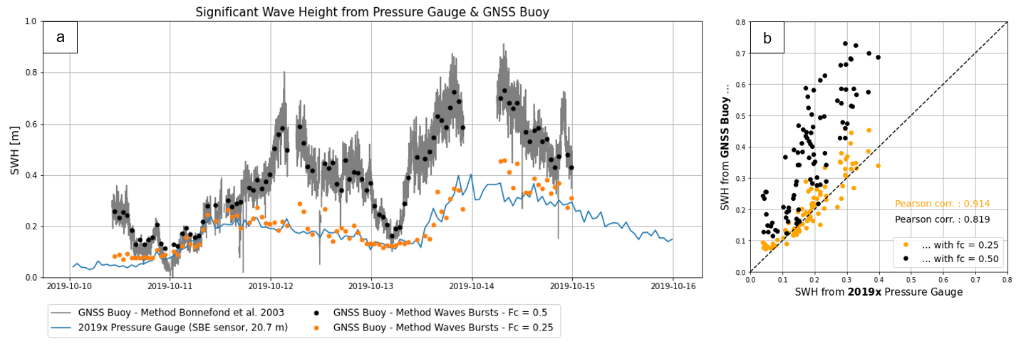
Figure D3 (a) Significant wave height (SWH) from GNSS buoy (grey line) and 2019× pressure gauge (blue line). To allow a direct comparison, the GNSS buoy SWH is also computed with the wave burst method, using different cutoff frequencies (black and orange points). (b) Correlation between 2019× pressure gauge and GNSS buoy SWH.

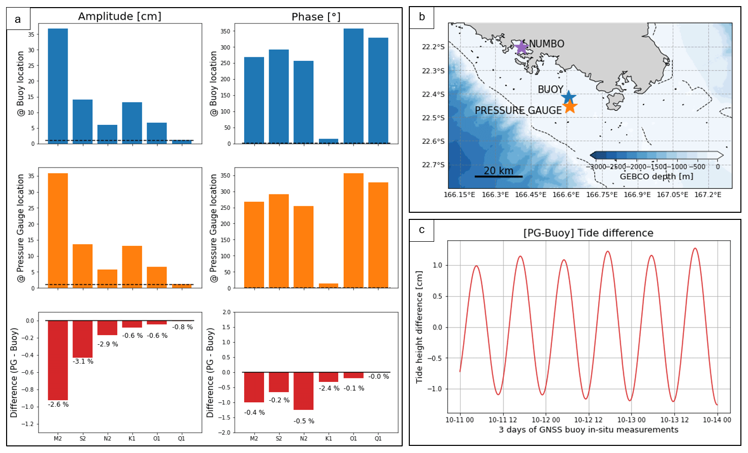
Figure D4 (a) Amplitude and phase of the six main tide constituents extracted from SCHISM hydrodynamic model at the buoy (blue) and pressure gauge location (orange). The red bar plot shows amplitude and the phase of the tide gradient between these two points. (b) Location of the sensors. Note that star colours correspond to bar plot colours. (c) Tide reconstruction over the 3 d of the GNSS buoy measurements using amplitude and phase of the tide gradient.

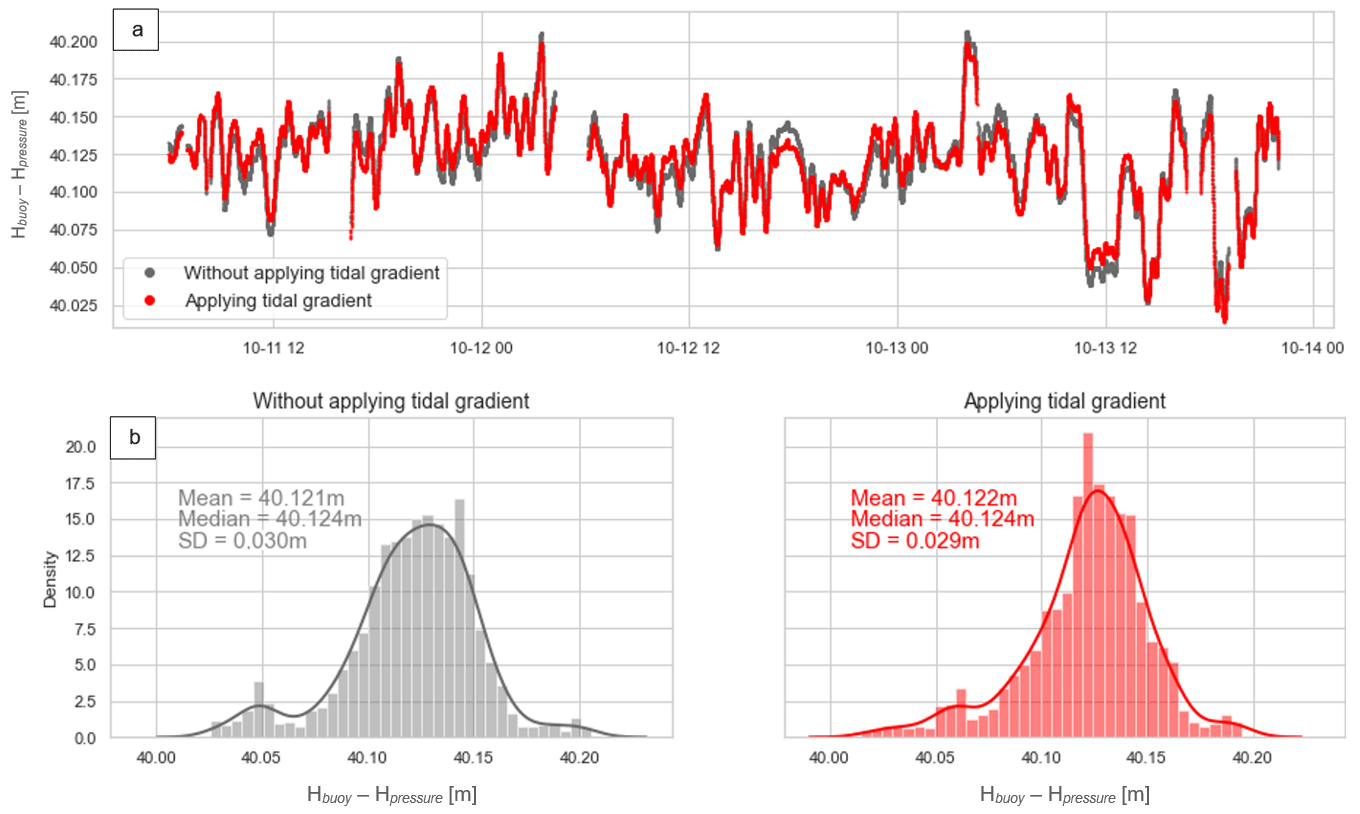
Figure D5 (a) Height difference over the 3 d of common observation period between the GNSS buoy and the pressure gauge (see Sect. 3.3 for more details) considering (in red) or not considering (in grey) the tide gradient between the two locations. (b) Histograms of the GNSS buoy and pressure gauge differences without (left panel – grey) or with (right panel – red) tide gradients.

Appendix E: Along-track altimetric wet tropospheric corrections

In the lagoon, the effect of coastal contamination on the radiometer data is visible when approaching the main island (Figs. E1 and E2 right panels, grey area). However, the wet tropospheric correction seems to be exploitable at our comparison point for all missions (Fig. E1, red area).

To test this hypothesis, we compared the correction provided by the radiometer with two datasets: (1) the wet tropospheric correction from the ECMWF model and (2) the wet tropospheric correction computed from permanent GNSS stations in Nouméa. For the latter, we used the total tropospheric delay extracted from GINS PPP computations, performed by the Centre National d'Etudes Spatiales (CNES) teams in Toulouse, for the NRMD and NOUM stations. The tropospheric corrections, estimated every 2 h, are interpolated at the satellite pass times. The dry tropospheric component from GDR files is then subtracted to finally obtain the wet component of the tropospheric correction. Since the GNSS stations are not at sea level elevation, an additional correction is applied to account for the pressure difference with the comparison point (which is at sea level elevation). For this, we used the Saastamoinen equations (Saastamoinen, 1972) according to the method described by Kouba (2008).

To illustrate the objective of our comparison, we represent the wet tropospheric delay from the radiometer, the ECMWF model, and GNSS data along Jason-3 track 162 for three random cycles (Fig. E3). If we focus on our study area (the grey area on Fig. E3), we can see that the three solutions can be very variable according to the cycles and can affect the estimate of the altimetric SSH at the centimetric level.

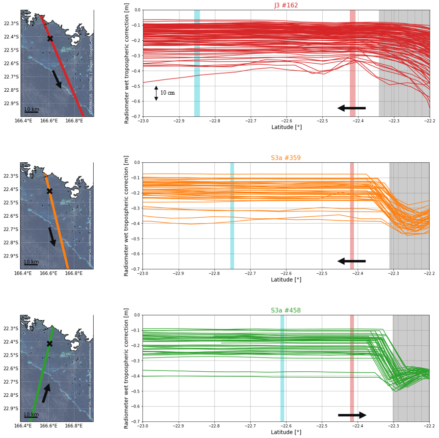
Figure E1 Evolution of the radiometer correction along the altimetric tracks used in our study (red for Jason-3 162, orange for Sentinel-3A 359 and green for Sentinel-3A 458). The grey vertical bar represents the main island overfly, the red vertical bar represents the comparison point location, and the blue vertical bar corresponds to the reef barrier overfly. Arrows symbolise the satellite direction of flight.

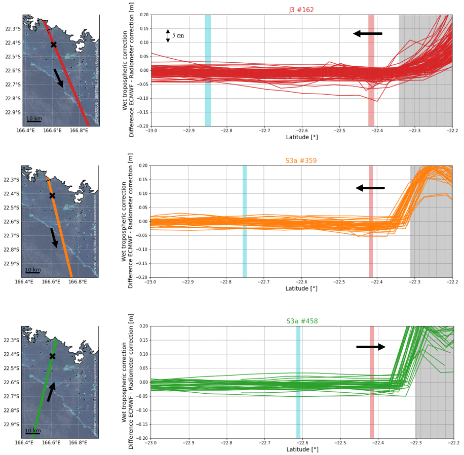
Figure E2 Evolution of the difference between ECMWF and the radiometer correction along the altimetric tracks used in our study (red for Jason-3 162, orange for Sentinel-3A 359 and green for Sentinel-3A 458). The grey vertical bar represents the main island overfly, the red vertical bar represents the comparison point location, and the blue vertical bar corresponds to the reef barrier overfly. Arrows symbolise the satellite direction of flight.

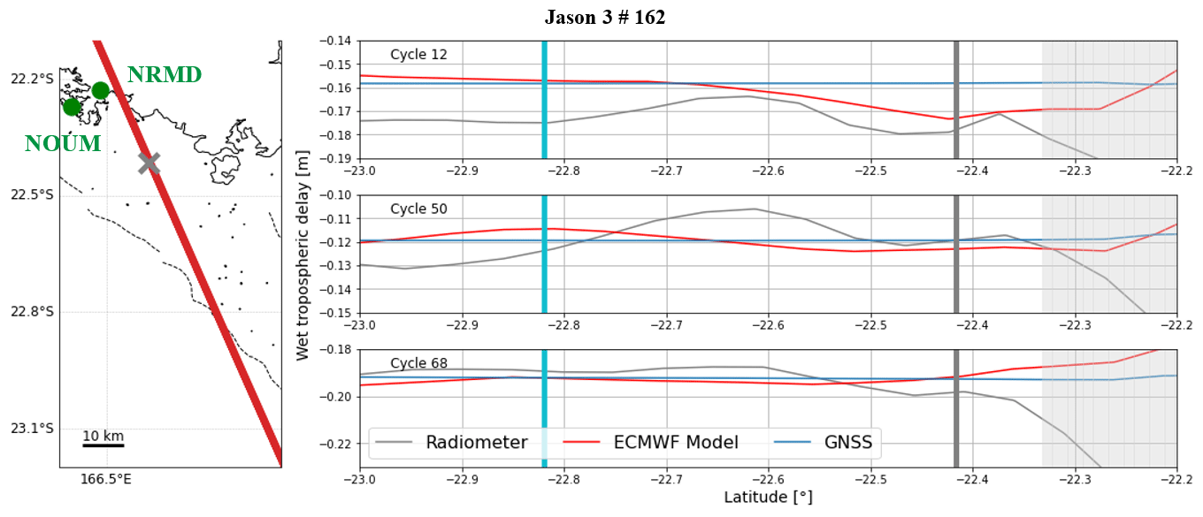
Figure E3 Wet tropospheric correction from radiometer (grey), ECMWF model (red), and GNSS stations (blue) for three random cycles of Jason-3 162. On the right panel, the light grey area represents the main island overfly, the dark grey area represents the comparison point overfly, and the blue area corresponds to the reef barrier overfly.

Appendix F: Validation of gradients from global geoïd models in the lagoon

Another objective of the cruise was to improve sea level kinematic mapping methodology in coastal areas through the deployment and comparison of multiple sensors, as described in Chupin et al. (2020). For that purpose, the coastal version of the CalNaGeo GNSS carpet was towed by R/V Alis along and across altimetry tracks and inside and outside the lagoon (Fig. 1b, blue lines). The 10 s observations of CalNaGeo were processed with GINS in PPP mode (Marty et al., 2011) (processing details in Appendix C) and filtered using the Vondrak filter with a cutoff period of 30 min (∼ 5.4 km at 6 knots). The 2019× pressure sensor is then used to remove the time-varying component of CalNaGeo measurements (especially the oceanic tide, assuming that it does not vary spatially over our area). Thanks to these data, we then analyse the performance of different models to estimate geoid gradients.

Three datasets were selected to conduct our comparison:

• The XGM2019e global gravity field model (Zingerle et al., 2020), represented by spherical harmonics corresponding to a spatial resolution of 2 arcmin (∼ 4 km), is based on GOCO06s satellite data combined with terrestrial measurements for shorter wavelengths. Gravity anomalies derived from satellite altimetry are used over oceans (DTU13).

• The global Earth gravity potential model EGM2008 (Pavlis et al., 2012) defined on a 5 arcmin (∼ 10 km) equiangular grid, is based on terrestrial, altimetric, and airborne gravity data.

• An average model of the Earth's gravity field, the EIGEN-GRGS.RL04.MEAN-FIELD (Lemoine et al., 2019), hereafter referred to as EIGEN, is computed from the RL04 GRACE+SLR monthly time series and GOCE data.

Along the CalNaGeo track, the comparison with XGM2019e and EGM08 gradients shows no significant differences (Fig. F1b and c, respectively). On the contrary, the comparison with the EIGEN model shows a residual southeast–northwest gradient of about 1.8 cm km⁻¹ (Fig. F1d). In our process, we thus select the XGM2019e model to account for geoid gradients. This first study allowed us to select the most relevant model for our area, but further analysis is still required to refine the CalNaGeo GNSS solution and to map the mean sea surface over the whole lagoon.

Table F1 Geoïd height difference between 2019× pressure gauge (4 km south of the crossover) and Nouméa tide gauge site.

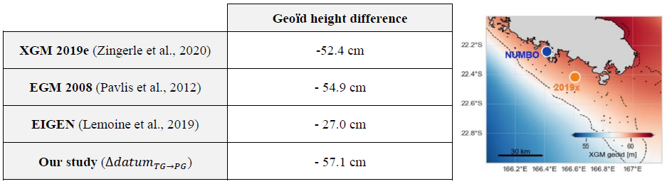
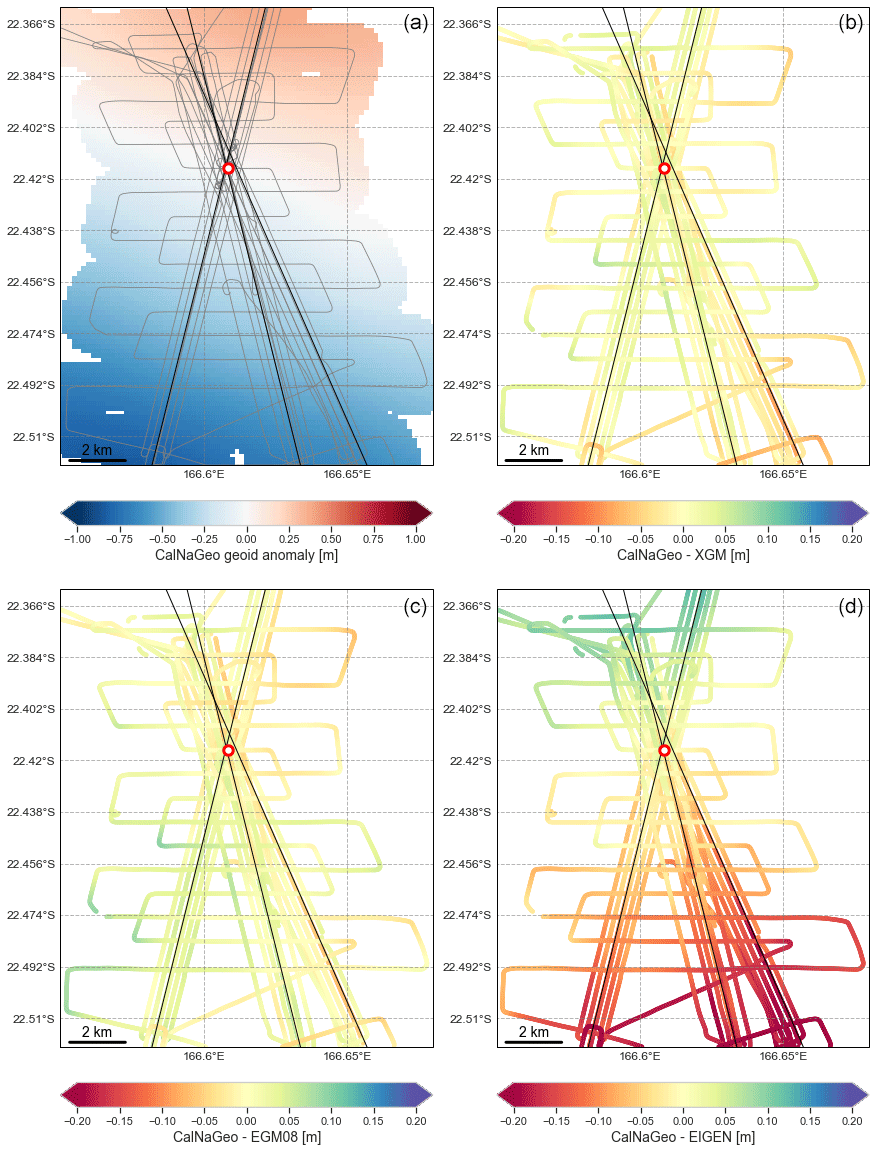
Figure F1 Comparison of global gravity field models with CalNaGeo measurements. (a) Mean sea surface anomalies from CalNaGeo measurements during the GEOCEAN-NC cruise, expressed with respect to the altimeter comparison point (red dot on the map). (b) Difference between CalNaGeo and the XGM2019e model with respect to the comparison point. (c) Difference between CalNaGeo and the EGM08 model with respect to the comparison point. (d) Difference between CalNaGeo and the EIGEN model with respect to the comparison point.

Appendix G: Assessment of altimetry data quality in the lagoon

The retracking provides the range by fitting a theoretical model on the radar echo recorded by the altimeter. The mean quadratic error (MQE) parameter gives one an idea of the retracking process: the closer the MQE is to zero, the better the chosen model reproduce the measured waveform. So far, altimetry products have not given any indication of a valid or invalid MQE value. To get an idea of the “threshold” value of the MQE parameter that could discriminate valid or invalid ocean waveforms, we conducted an analysis on two Jason-3 and two Sentinel-3A tracks. For all cycles between 2016 and 2019, we extract along-track 20 Hz MQE parameters and compare them to the coastline distance.

For Jason-3, our analysis shows that in the open ocean (i.e. distance to the coast > 30 km), the mean MQE parameter is less than or equal to 0.01 (Fig. G2, red and orange). Along the Sentinel-3A tracks, this mean MQE value is more variable with a standard deviation of ∼ 2 and 2.5 (compared to 0.04 and 0.07 for Jason). However, the median is well below 0.01, suggesting that extreme values influence the estimate of the mean (Fig. G2, grey and black). Approaching the coast, the MQE parameter increases significantly (Fig. G3). In the 10–15 km range, the mean MQE tends towards 0.01 for Jason, but it tends towards 0.1 for Sentinel (Fig. G3). We could therefore consider that MQE values greater than 0.01 could indicate an improper retracking and therefore potentially erroneous water depths. These preliminary results are strongly influenced by the tracks geometry, and a global analysis of all satellite passes would help to determine a more realistic threshold value for each mission.

However, to analyse our dataset, we considered that a MQE value above 0.01 may indicate a non-oceanic radar signal for both Jason and Sentinel missions. Figure G4 shows the 20 Hz along-track MQE parameter for the three tracks over the year 2019. There are about 3 times more Jason than Sentinel data because of the difference in revisit period (9.9 and 27 d for Jason-3 and Sentinel satellites, respectively). We can note that, for each track, the MQE parameter is higher and more variable at the coral reef overfly (dotted black line). Closer to the coast, the MQE parameter in the crossover area (black box) is mostly below 0.01, indicating that the waveform retracking using the open-ocean model is suitable for most passes. As the retracking allows the determination of the altimeter range, and thus the computation of the altimeter sea surface height, this result supports the idea that SSH altimetry data in our comparison area are reliable.

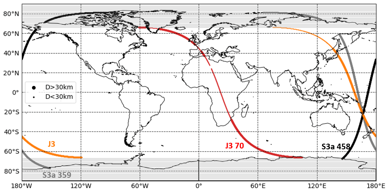
Figure G1 Distance to nearest coastline from the along-track point of the two Jason and two Sentinel tracks used to analyse the MQE parameter. The big dots represent along-track points more than 30 km away from the nearest coastline, and the small dots are points located on land or less than 30 km from the coastline. Note that to have a consistent comparison between both missions, Sentinel points located in polar areas (between [−90^∘, −66^∘] and [90^∘, 66^∘] areas) are not considered in the computation.

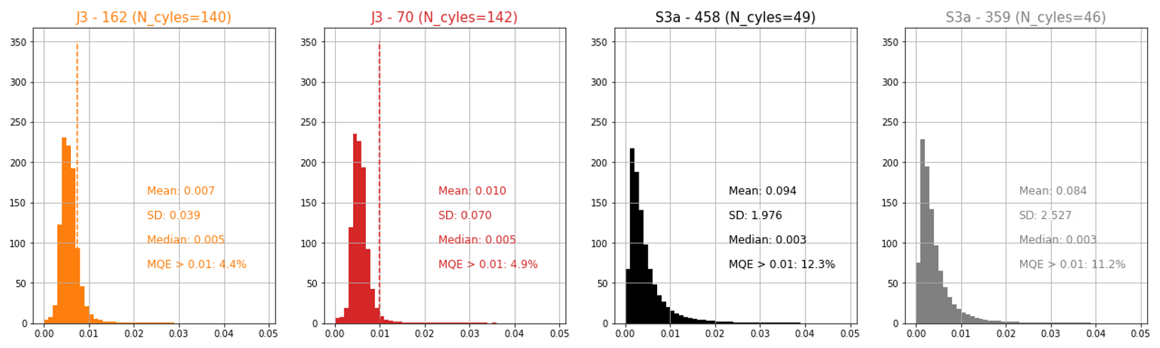
Figure G2 Statistics on the MQE values of points located more than 30 km from the coast (considered oceanic points). The dashed line represents the mean value.

Figure G3 Mean values of MQE parameter function of the distance to the coast.

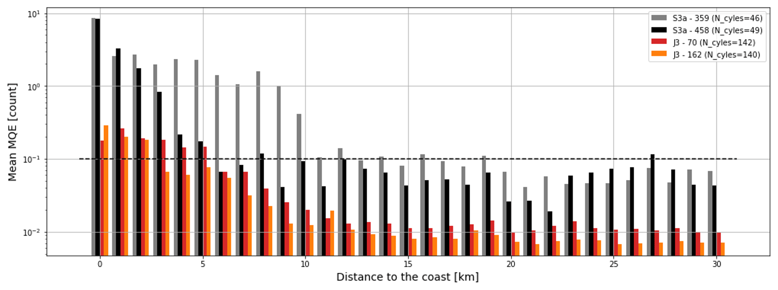
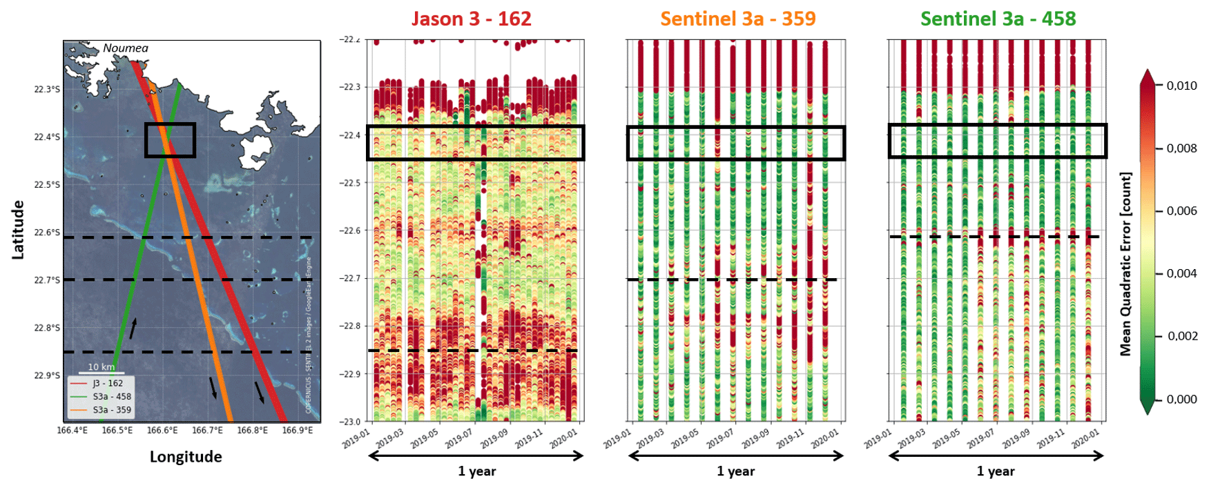
Figure G4 Along-track mean quadratic error (MQE) parameter for the three satellites passes that cross the lagoon during year 2019. The grey area represents the crossing area, and the dotted black lines indicate the open-ocean–lagoon interface for each track.